DFF 383/3/02

March 2002

Geometric scaling and QCD evolution
J.  Kwieciński^(a) and A. M.  Staśto^(a,b)

^(a)H. Niewodniczański Institute of Nuclear Physics, Kraków, Poland

^(b) INFN Sezione di Firenze, Via G. Sansone 1, 50019 Sesto Fiorentino (FI), Italy

()

We study the impact of the QCD DGLAP evolution on the geometric scaling of the gluon distributions which is expected to hold at small $x$ within the saturation models. To this aim we solve the DGLAP evolution equations with the initial conditions provided along the critical line $Q^{2}=Q_{s}^{2}(x)$ with $Q_{s}^{2}(x)\sim x^{-\lambda}$ and satisfying geometric scaling. Both fixed and running coupling cases are studied. We show that in the fixed coupling case the geometric scaling at low $x$ is stable against the DGLAP evolution for sufficiently large values of the parameter $\lambda$ and in the double logarithmic approximation of the DGLAP evolution this happens for $\lambda\geq 4N_{c}\alpha_{s}/\pi$. In the running coupling case geometric scaling is found to be approximately preserved at very small $x$. The residual geometric scaling violation in this case can be approximately factored out and the corresponding form-factor controlling this violation is found.

1 Introduction

Perturbative QCD predicts very strong power-law rise of the gluon density $xg(x,Q^{2})$ in the limit $x\rightarrow 0$, where, as usual, $x$ denotes the momentum fraction carried by the gluon and $Q^{2}$ is the scale at which the distribution is probed. This strong rise can eventually violate unitarity and so it has to be tamed by screening effects. Those screening effects are provided by multiple parton interactions which lead to the non-linear terms in the (BFKL and/or DGLAP) equations [1] - [13]. These non-linear terms reduce the growth of gluon distributions and generate instead the parton saturation at sufficiently small values of $x$ and/or $Q^{2}$ [1] - [20].

Increase of the gluon distribution and emergence of the saturation effects imply similar properties of the measurable quantities which are driven by the gluon, like the deep inelastic structure function $F_{2}(x,Q^{2})$. This can be most clearly seen in the dipole picture of deep inelastic scattering in which the virtual photon - proton total cross section $\sigma_{\gamma^{*}p}(x,Q^{2})$ ( $\sigma_{\gamma^{*}p}(x,Q^{2})\sim F_{2}(x,Q^{2})/Q^{2})$) is linked with the cross section $\sigma_{dp}(x,r)$ describing the interaction of the $q\bar{q}$ colour dipole with the proton, where $r$ denotes the transverse size of the dipole [3, 21, 22, 25]. The dipole-proton cross section is determined by the gluon distribution in the proton and in leading order approximation we just have $\sigma_{dp}(x,r)\sim\alpha_{s}(1/r^{2})r^{2}xg(x,1/r^{2})$. Increase and/or saturation of the gluon distribution in the small $x$ limit implies similar increase and/or saturation of the dipole-proton cross section and of the cross-section $\sigma_{\gamma^{*}p}(x,Q^{2})$.

The successful description of all inclusive and diffractive deep inelastic data at HERA by the saturation model [22] ( see also [23] and [24]) suggests that the screening effects might become important in the energy regime probed by the present colliders. Important property of the dipole cross section which holds in this model is its geometric scaling, i.e. dependence upon single variable $\tau=r^{2}Q_{s}^{2}(x)$ where $Q_{s}(x)$ is the saturation scale. This leads to the geometric scaling of $\sigma_{\gamma^{*}p}(x,Q^{2})$ itself, i.e. $\sigma_{\gamma^{*}p}(x,Q^{2})=f(Q^{2}/Q_{s}^{2}(x))$ which is well supported by the experimental data from HERA [26]. Geometric scaling of the dipole cross-section should imply similar scaling of the quantity $\alpha_{s}(Q^{2})xg(x,Q^{2})/Q^{2}$. This type of scaling is also found to be an intrinsic property of the non-linear evolution equations [6, 8], [11] - [20]. It turns out that for the equations of type

$$\frac{\partial\phi(x,k)}{\partial\ln(1/x)}\,=\,{\bar{\alpha}_{s}}K\otimes\phi-{\bar{\alpha}_{s}}\phi^{2}(x,k)\;,\hskip 28.45274pt({\bar{\alpha}_{s}}\equiv\frac{N_{c}\alpha_{s}}{\pi})\;,$$ (1)

where $K$ is a linear evolution kernel (for example of BFKL type) there exist a region in $x$ and $k$ space such that

$$\phi(x,k)=\phi(Q_{s}^{2}(x)/k^{2})\hskip 14.22636pt{\rm for}\hskip 14.22636ptk^{2}<Q_{s}^{2}(x)\;.$$ (2)

For example in the case of the Balitsky-Kovchegov [11, 12] equation, where $K$ is the BFKL kernel, the saturation scale $Q_{s}^{2}(x)$ has been found to have a general power like dependence on $x$ , $Q_{s}^{2}(x)=Q_{0}^{2}x^{-\lambda}$. The coefficient $\lambda$ which is approximately equal to $4{\bar{\alpha}_{s}}$ in this case, is then a universal quantity and does not depend on the initial conditions for the evolution [16] - [20].

The main purpose of this paper is to analyse possible compatibility of this scaling with the DGLAP evolution equations. It is expected that the non-linear shadowing effects should be weak in the region ’to the right’ of the critical line defined by the saturation scale $Q_{s}^{2}(x)$ , i.e. for $Q^{2}>Q_{s}^{2}(x)$, see Fig. 1. In order to study possible impact of the DGLAP evolution we shall therefore assume the geometric scaling parametrisation along the critical line and inspect the structure of the solution of the DGLAP equation with those initial conditions. This way of providing the initial conditions along the critical line $Q^{2}=Q_{s}^{2}(x)$ rather than at $Q^{2}=Q_{0}^{2}$ with $x$ independent reference scale $Q_{0}^{2}$ is the characteristic feature of the saturation effects [1].

The content of our paper is as follows. In the next section we give semianalytical insight into the solution of the DGLAP equation with the starting distributions provided along the critical line. We study separately the fixed and running coupling cases. In Section 3 we present numerical analysis of our solutions and finally in Section 4 we give our conclusions.

2 Solution of the DGLAP equations from the starting distributions provided along the critical line

We wish to understand possible effects of the DGLAP evolution on the geometric scaling at low $x$. This scaling means that certain quantities controlling deep inelastic scattering at low $x$, like the dipole-proton cross section $\sigma_{dp}(x,r=1/Q)$ or the virtual photon-proton cross section $\sigma_{\gamma^{*}p}$, which are in principle functions of two variables, depend upon the single variable $Q/Q_{s}(x)$. The saturation scale $Q_{s}(x)$, which also specifies the critical line increases with decreasing $x$

$$Q_{s}^{2}(x)=Q_{0}^{2}x^{-\lambda}\;.$$ (3)

Let us assume that:

1. For $Q^{2}<Q_{s}^{2}(x)$ the linear evolution is strongly perturbed by the nonlinear effects which generate geometric scaling for the dipole cross section $\sigma_{dp}(x,r=1/Q)$ and for the related quantities.

2. Geometric scaling for the dipole cross-section implies geometric scaling for
   $\alpha_{s}(Q^{2})xg(x,Q^{2})/Q^{2}$, where $g(x,Q^{2})$ denotes the gluon distribution. This follows from the LO relation between the dipole cross section and the gluon distribution, i.e. $\sigma(x,r^{2})\sim r^{2}\alpha_{s}(1/r^{2})xg(x,1/r^{2})$.

3. Geometric scaling for $\alpha_{s}(Q^{2})xg(x,Q^{2})/Q^{2}$ holds at the boundary $Q^{2}=Q_{s}^{2}(x)$.

4. For $Q^{2}>Q_{s}^{2}(x)$ the non-linear screening effects can be neglected and evolution of parton densities is governed by the DGLAP equations.

We wish to study possible effects of the DGLAP evolution upon the geometric scaling in the region $Q^{2}>Q_{s}^{2}(x)$ after solving the linear DGLAP evolution equations starting from the gluon distribution satisfying this scaling and defined along the critical line $Q_{s}^{2}(x)$ (see point 3 above). We shall discuss the fixed and running coupling cases separately.

2.1 The fixed coupling case

Let us consider standard leading order evolution of the gluon distribution $xg(x,Q^{2})$

$${\partial xg(x,Q^{2})\over\partial\ln(Q^{2}/\Lambda^{2})}={\alpha_{s}\over 2\pi}\int_{x}^{1}{dz\over z}P_{gg}(z)\;xg(x/z,Q^{2})\;,$$ (4)

where, as usual, the $P_{gg}$ is the gluon-gluon splitting function. For simplicity we have neglected possible contribution of the quark distributions. In the moment space this equation has the following form

$${\partial g_{\omega}(Q^{2})\over\partial\ln(Q^{2}/\Lambda^{2})}={\alpha_{s}\over 2\pi}\gamma_{gg}(\omega)g_{\omega}(Q^{2})\;,$$ (5)

where we have defined the Mellin transform to be

$$g_{\omega}(Q^{2})=\int_{0}^{1}dx\,x^{\omega}g(x,Q^{2})\;,$$ (6)

and the gluon anomalous dimension is defined as

$$\gamma_{gg}(\omega)\;=\;\int_{0}^{1}dz\,z^{\omega}P_{gg}(z)\;.$$ (7)

The solution of equation (5) is straightforward and given by

$$g_{\omega}(Q^{2})=g_{0}(\omega)\left({Q^{2}\over Q_{0}^{2}}\right)^{{\alpha_{s}\over 2\pi}\gamma_{gg}(\omega)}\;.$$ (8)

We will now seek equation for the moment function $g_{0}(\omega)$ using the following initial condition

$${\alpha_{s}\over 2\pi}xg(x,Q^{2}=Q_{s}^{2}(x))={\alpha_{s}\over 2\pi}r^{0}x^{-\lambda}\;,$$ (9)

where $Q_{s}^{2}(x)$ is given by equation (3). The parameter $r^{0}$ specifies the normalisation of gluon distribution along the critical line. This boundary condition follows from the geometric scaling condition of the dipole proton cross section $\sigma_{dp}(r=1/Q,x)$ which is proportional to $\alpha_{s}xg(x,Q^{2})/Q^{2}$.

In order to find solution for $g_{0}(\omega)$ we use the inverse Mellin transform

$$xg(x,Q^{2})={1\over 2\pi i}\int d\omega\,x^{-\omega}g_{\omega}(Q^{2})\;,$$ (10)

where the integration contour should be located to the right of the singularities of $g_{\omega}(Q^{2})$ in the $\omega$ plane. Inserting in equation (10) the DGLAP solution (8) for $g_{\omega}(Q^{2})$ we get

$$xg(x,Q^{2})={1\over 2\pi i}\int d\omega\,x^{-\omega}g_{0}(\omega)\left({Q^{2}\over Q_{0}^{2}}\right)^{{\alpha_{s}\over 2\pi}\gamma_{gg}(\omega)}\;.$$ (11)

We now set $Q^{2}=Q_{s}^{2}(x)$ with the saturation scale $Q_{s}^{2}(x)$ defined by equation (3), and require the geometric scaling initial condition along the critical line $Q^{2}=Q_{s}^{2}(x)$ (see eq. (9)). From equations (3),(9) and (11) we get

$${1\over 2\pi i}\int d\omega g_{0}(\omega)x^{-\omega-\lambda{\alpha_{s}\over 2\pi}\gamma_{gg}(\omega)}=r^{0}x^{-\lambda}\;.$$ (12)

This equation can be regarded as the equation for the function $g_{0}(\omega)$, i.e. for the moment of the gluon distribution at the ($x$ independent) scale $Q_{0}^{2}$. In order to solve this equation we take the moment of both sides of equation (12), i.e. we integrate both sides of this equation over $dx$ for $0<x<1$ with the weight $x^{\omega_{1}-1}$ and get

$${1\over 2\pi i}\int d\omega{g_{0}(\omega)\over[\omega_{1}-\omega-\lambda{\alpha_{s}\over 2\pi}\gamma_{gg}(\omega)]}={r^{0}\over\omega_{1}-\lambda}\;.$$ (13)

We now change the integration variables

$$z=\omega+\lambda{\alpha_{s}\over 2\pi}\gamma_{gg}(\omega)\;,$$ (14)

which after inversion specifies the function $\omega(z)$. Equation (13) in the new variable $z$ takes then the following form

$${1\over 2\pi i}\int dz{d\omega(z)\over dz}{g_{0}(\omega(z))\over(\omega_{1}-z)}={r^{0}\over\omega_{1}-\lambda}\;.$$ (15)

We can easily perform the contour integration in Eq.(15) and get

$${d\omega(z)\over dz}\bigg{|}_{z=\omega_{1}}g_{0}(\omega(z=\omega_{1}))={r^{0}\over\omega_{1}-\lambda}\;.$$ (16)

We still need to solve this equation for $g_{0}(\omega)$ and in order to do this we write

$$\omega_{1}=\omega+\lambda{\alpha_{s}\over 2\pi}\gamma_{gg}(\omega)\;,$$ (17)

and finally from Eq.(16) we obtain

$$g_{0}(\omega)=[1+\lambda{\alpha_{s}\over 2\pi}{d\gamma_{gg}(\omega)\over d\omega}]{r^{0}\over[\omega+\lambda{\alpha_{s}\over 2\pi}\gamma_{gg}(\omega)-\lambda]}\;,$$ (18)

which defines the solution for $g_{0}(\omega)$.

In what follows it is convenient to use directly redefined function $\tilde{g}_{0}(z)$

$$\tilde{g}_{0}(z)\equiv{d\omega(z)\over dz}g_{0}(\omega(z))\;,$$ (19)

where from equation (16) we see that

$$\tilde{g}_{0}(z)={r^{0}\over z-\lambda}\;.$$ (20)

The solution of the DGLAP equation with the initial condition specified by equation (9) then reads

$$xg(x,Q^{2})={1\over 2\pi i}\int dzx^{-z}\tilde{g}_{0}(z)\left({Q^{2}\over Q_{s}^{2}(x)}\right)^{{\alpha_{s}\over 2\pi}\gamma_{gg}(\omega(z))}$$ (21)

where the integration contour is located to the right of the singularities of $\tilde{g}_{0}(z)$ and of $\omega(z)$. If the leading singularity is a pole of $\tilde{g}_{0}(z)$ at $z=\lambda$ then the leading contribution to $xg(x,Q^{2})$ at small $x$ is given by

$$xg(x,Q^{2})\simeq r^{0}x^{-\lambda}\left({Q^{2}\over Q_{s}^{2}(x)}\right)^{{\alpha_{s}\over 2\pi}\gamma_{gg}(\omega_{0})}\;,$$ (22)

where

$$\omega_{0}=\omega(\lambda)\;.$$ (23)

It should be noted that $\omega_{0}$ defines position of the pole of $g_{0}(\omega)$. In general we have $\omega_{0}\leq\lambda$. From equation (22) we get the following leading small $x$ behaviour for the gluon density ${\alpha_{s}\over 2\pi}xg(x,Q^{2})/Q^{2}$

$${\alpha_{s}\over 2\pi}{xg(x,Q^{2})\over Q^{2}}\simeq{r^{0}\over Q_{0}^{2}}{\alpha_{s}\over 2\pi}\left({Q^{2}\over Q_{s}^{2}(x)}\right)^{{\alpha_{s}\over 2\pi}\gamma_{gg}(\omega_{0})-1}\;,$$ (24)

which respects the geometric scaling i.e. is a function of only one combined variable $Q^{2}/Q_{s}^{2}(x)$. Violation of this scaling by the contribution of the (branch point) singularity of $\omega(z)$ is a non-leading effect at low $x$.

The requirement that the pole of $\tilde{g}^{0}(z)$ at $z=\lambda$ is the leading singularity imposes certain constraints upon $\lambda$. In general they are difficult to be found exactly since the inversion of equation (14) cannot be performed analytically when using complete form of $\gamma_{gg}(\omega)$. Analytic solution of equation (14) is however possible in the double logarithmic approximation in which $\gamma_{gg}(\omega)=\gamma_{gg}^{DL}(\omega)$, where

$$\gamma_{gg}^{DL}(\omega)={2N_{c}\over\omega}\;,$$ (25)

is the most singular in $\omega\rightarrow 0$ part of the gluon anomalous dimension $\gamma_{gg}(\omega)$. In this approximation we get

$$\omega(z)={z+\sqrt{z^{2}-4\bar{\alpha}_{s}\lambda}\over 2}\;,$$ (26)

where

$$\bar{\alpha}_{s}={N_{c}\alpha_{s}\over\pi}\;.$$ (27)

We also have

$$\omega_{0}={\lambda+\sqrt{\lambda^{2}-4\bar{\alpha}_{s}\lambda}\over 2}\;.$$ (28)

The condition that the pole of $\tilde{g}^{0}(z)$ at $z=\lambda$ is the leading singularity, i.e. that it is located to the right of the branch-point singularity of $\omega(z)$ at $z=2\sqrt{\bar{\alpha}_{s}\lambda}$ gives the following constraint upon the parameter $\lambda$

$$\lambda\geq 4\bar{\alpha}_{s}\;.$$ (29)

For $\lambda<4\bar{\alpha}_{s}$ the leading singularity is the branch point of $\omega(z)$ at $z=2\sqrt{\bar{\alpha}_{s}\lambda}$ and the geometric scaling becomes violated.

It may be interesting to confront our results for the fixed coupling with the properties of the exact solution of the non-linear Balitsky - Kovchegov equation [20]. In this case geometric-scaling holds for $Q^{2}\leq Q_{s}^{2}(x)$ and the non-linear effects can be neglected for $Q^{2}>Q_{s}^{2}(x)$. The parameter $\lambda$ specifying the critical line is however not an independent quantity and depends upon the (fixed) coupling $\alpha_{s}$. In the double logarithmic approximation it is given by $\lambda=4\bar{\alpha}_{s}$. It follows from equation (29) that this is a limiting value of the parameter $\lambda$ for the geometric scaling to hold asymptotically in the small $x$ limit and so for $\lambda=4\bar{\alpha}_{s}$ we expect violation of this scaling for $Q^{2}>Q_{s}^{2}(x)$ down to the very small values of $x$ [20].

2.2 Running coupling case

We now pass to the more realistic case with the running coupling. In this case the evolution equation for the moment function takes the form:

$${\partial g_{\omega}(Q^{2})\over\partial\ln(Q^{2}/\Lambda^{2})}={\alpha_{s}(Q^{2})\over 2\pi}\gamma_{gg}(\omega)g_{\omega}(Q^{2})\;,$$ (30)

where the running coupling in the leading order is given by

$${\alpha_{s}(Q^{2})\over 2\pi}={b\over\ln(Q^{2}/\Lambda^{2})}\;,$$ (31)

with

$$b={2\over 11-2/3N_{f}}\;,$$ (32)

with $N_{f}$ being number of flavours. In this section we consider only gluonic channel therefore we set $N_{f}=0$. The solution of equation (30) reads

$$g_{\omega}(Q^{2})=g_{0}(\omega)\left({\ln(Q^{2}/\Lambda^{2})\over\ln(Q_{0}^{2}/\Lambda^{2})}\right)^{b\gamma_{gg}(\omega)}\;.$$ (33)

From the above solution we obtain

$${\alpha_{s}(Q^{2})\over 2\pi}g_{\omega}(Q^{2})={\alpha_{s}(Q_{0}^{2})\over 2\pi}g_{0}(\omega)\left({\ln(Q^{2}/\Lambda^{2})\over\ln(Q_{0}^{2}/\Lambda^{2})}\right)^{b\gamma_{gg}(\omega)-1}\;,$$ (34)

and so the result for the gluon distribution $xg(x,Q^{2})$ in $x$ space reads in this case

$${\alpha_{s}(Q^{2})\over 2\pi}xg(x,Q^{2})={1\over 2\pi i}\int d\omega x^{-\omega}f_{0}(\omega)\left({\ln(Q^{2}/\Lambda^{2})\over\ln(Q_{0}^{2}/\Lambda^{2})}\right)^{b\gamma_{gg}(\omega)-1}\;,$$ (35)

where

$$f_{0}(\omega)={\alpha_{s}(Q_{0}^{2})\over 2\pi}g_{0}(\omega)\;.$$ (36)

We now impose the geometric scaling condition (9) onto this solution to get

$${1\over 2\pi i}\int d\omega x^{-\omega}f_{0}(\omega)\left(1+{\lambda\ln(1/x)\over\ln(Q_{0}^{2}/\Lambda^{2})}\right)^{b\gamma_{gg}(\omega)-1}=r^{0}x^{-\lambda}\;.$$ (37)

which is an equation for $f_{0}(\omega)$. Solution of this equation is complicated, i.e. exact solution generates complicated (branch point) singularity of $f_{0}(\omega)$ at $\omega=\lambda$. The only observation which we can make is that it should generate $x^{-\lambda}$ behaviour softened by inverse powers of the $\ln(1/x)$. In order to make some insight into what is going on we have to make some approximations. To be precise let us make the approximation by setting $\omega=\lambda$ in the argument of $\gamma_{gg}(\omega)$ that gives

$${1\over 2\pi i}\int d\omega x^{-\omega}f_{0}(\omega)\simeq\left(1+{\lambda\ln(1/x)\over\ln(Q_{0}^{2}/\Lambda^{2})}\right)^{-(b\gamma_{gg}(\lambda)-1)}\!\!r^{0}x^{-\lambda}\;.$$ (38)

Making the same approximation in the inverse Mellin transform (35) we get the solution

$${\alpha_{s}(Q^{2})\over 2\pi}xg(x,Q^{2})\simeq x^{-\lambda}r^{0}\left({\ln(Q^{2}/\Lambda^{2})\over\ln(Q_{0}^{2}/\Lambda^{2})}\right)^{b\gamma_{gg}(\lambda)-1}\left(1+{\lambda\ln(1/x)\over\ln(Q_{0}^{2}/\Lambda^{2})}\right)^{-(b\gamma_{gg}(\lambda)-1)}\,.$$ (39)

Multiplying and dividing $Q^{2}$ by $Q_{0}^{2}x^{-\lambda}$ we finally obtain

$${\alpha_{s}(Q^{2})\over 2\pi}xg(x,Q^{2})=x^{-\lambda}r^{0}\left({\ln(Q^{2}x^{\lambda}/Q_{0}^{2})\over\ln(Q_{0}^{2}/\Lambda^{2})+\lambda\ln(1/x)}+1\right)^{b\gamma_{gg}(\lambda)-1}\;.$$ (40)

The factor proportional to $\ln(1/x)$ in the denominator of the expression on the r.h.s. of (40) generates violation of the geometric scaling. Thus in the case of running of the coupling $\alpha_{s}(Q^{2})$ the scaling behaviour gets violated, it is possible however to factor out the effect of this violation. We can also rewrite Eq.(40) by using the definition of the saturation scale and the running coupling to get

$${\alpha_{s}(Q^{2})\over 2\pi}{xg(x,Q^{2})\over Q^{2}}\;=\;{r^{0}\over Q_{0}^{2}}{Q_{s}^{2}(x)\over Q^{2}}\left[1+\frac{\alpha_{s}(Q_{s}^{2}(x))}{2\pi b}\ln(Q^{2}/Q_{s}^{2}(x))\right]^{b\gamma_{gg}(\lambda)-1}\;,$$ (41)

where we see that the violation is proportional to the value of the running coupling evaluated at the saturation scale. Consequently when $x\ll 1$ that is when $Q_{s}(x)\gg 1$ the geometric scaling is restored, provided of course that $\alpha_{s}(Q_{s}^{2}(x))\ln(Q^{2}/Q_{s}^{2}(x))\ll 1$ as well. This condition is equivalent to $\ln(Q^{2}/Q_{s}^{2}(x))\ll\ln(Q_{s}^{2}(x)/\Lambda^{2})$. The same condition defining the region in which the geometric scaling holds above the saturation scale has recently been found in ref. [27].

3 Numerical results

In this section we present numerical results for the evolution of ordinary DGLAP equations for the integrated gluon distribution function with special boundary conditions set on the critical line $Q_{s}^{2}(x)$ as described in Sec.1.

3.1 Fixed coupling case

We start with the simplest case which is the fixed strong coupling. We assume also in the first approximation the DLLA limit that is we only keep the most singular part of the $P_{gg}$ splitting function in our simulation i.e.

$$P_{gg}(z)=\frac{2N_{c}}{z},\;\;N_{c}=3\;,$$ (42)

which results in the following form for the anomalous dimension of Eq.(7)

$$\gamma_{gg}(\omega)=\frac{2N_{c}}{\omega}\;.$$ (43)

The initial condition for the evolution of the gluon density is assumed to be of the form (9). We take $\lambda=0.5$ and $\alpha_{s}=0.1$. In Fig.2 we show the results of the calculation in this case. We illustrate the scaling behaviour of the gluon density by plotting $xg(x,Q^{2})/Q^{2}$ versus scaling variable $\tau=Q^{2}/Q_{s}^{2}(x)$ for different values of rapidity $Y=\ln 1/x$. From Eq.(24) we see that this function should scale with $\tau=Q^{2}/Q_{s}^{2}(x)$. The geometric scaling would correspond in this plot (Fig. 2) to the perfect overlap of all curves for different values of $Y$, so that they would form one single line. We see that up to a good accuracy this function does not depend dramatically on $Y$ and thus on $x$. We do however observe that there is some violation of the scaling at large $x$. This is due to the fact that the geometric scaling expression defined by equation (24) is only expected to hold asymptotically in the small $x$ limit. At finite $x$ this leading behaviour is perturbed by the non-leading contribution given by the branch-point singularity of $\omega(z)$ at $z=2\sqrt{\bar{\alpha}_{s}}$ , (see eq. (26) ).

To illustrate better the scaling and its violation we have plotted $xg(x,Q^{2})/Q^{2}$ versus scaling variable $\tau=Q^{2}/Q_{s}^{2}(x)$ using double-logarithmic scale, see Fig. 3a. One clearly sees that with increasing rapidity $Y$ the curves do not change and reach asymptotic straight line. We have also selected the very low $x$ range of Fig. 3a, which is Fig. 3b. One can see that in this case the geometric scaling is nearly preserved (we see nearly single line for different rapidities).

The behaviour of $xg(x,Q^{2})/Q^{2}$ versus $\tau=Q^{2}/Q_{s}^{2}(x)$ is clearly governed by a power law, with a power which we estimated to be approximately $-0.77$. From equation (24) and (28), and using the values of $\lambda$ and $\alpha_{s}$ quoted above we get that the power should be $\frac{\alpha_{s}}{2\pi}\gamma_{gg}(\omega_{0})-1=-0.74$ which is in a very good agreement with numerical result.

Let us note that in the case of DLLA (43), $\omega_{0}$ is a solution of the quadratic equation and is given by (28). As previously noticed the real solution exists only for $\lambda\geq\lambda_{min}=4\bar{\alpha_{s}}$ with $\bar{\alpha}_{s}=\alpha_{s}N_{c}/\pi$. We have numerically checked that for $\lambda\leq\lambda_{min}$ our solution no longer exhibits geometric scaling. It is interesting to note, as we have already observed at the end of Sec. 2.1, that exactly the same value of $\lambda=\lambda_{min}$ for a power of saturation scale was obtained from the studies of the nonlinear Balitsky-Kovchegov equation [11, 12] performed in [16] - [20].

We next abandon the DLLA approximation and consider more general case with the full gluon-gluon splitting function $P_{gg}$ which gives the following anomalous dimension

$$\gamma_{gg}(\omega)\;=\;2N_{c}\left[\frac{1}{\omega}-\frac{1}{\omega+1}+\frac{1}{\omega+2}-\frac{1}{\omega+3}-\gamma_{E}+\frac{11}{12}-\psi(\omega+2)\right]\;,$$ (44)

where $\psi$ is Polygamma function. In this case equation (14) with $z=\lambda$ can no longer be solved analytically and has to be analysed numerically. However, one can get insight into the allowed values of $\lambda$ by making the expansion of the anomalous dimension around $\omega=0$. In this case $\gamma_{gg}(\omega)/(2N_{c})\simeq\frac{1}{\omega}+A_{1}(0)+{\cal O}(\omega)$ where $A_{1}(0)=-\frac{11}{12}$. Using this approximation in (14) one finds that now geometric scaling will hold if the following condition is satisfied

$$\lambda\geq\lambda_{min}=\frac{4\bar{\alpha_{s}}}{[1-\bar{\alpha_{s}}A_{1}(0)]^{2}}\;.$$ (45)

We have checked numerically that above approximation works very well and gives very close results to the solution of (14) with full $\omega$ dependence of anomalous dimension $\gamma_{gg}(\omega)$.

In Fig.4a we plot $xg(x,Q^{2})/Q^{2}$ as a function of scaling variable $Q^{2}/Q_{s}^{2}(x)$ in the case of calculation with the full anomalous dimension (44). We have taken $\lambda=0.5$, and $\bar{\alpha}_{s}=0.1$. We see that the function exhibits geometric scaling (although there is some residual violation at larger values of $x$). The calculated value of exponent from numerical calculation is $-0.85$ which is again in nearly perfect agreement with the analytical estimate based on the approximation described above which gives $-0.86$. We also present in Fig. 4b the calculation in the case of $\lambda=0.3$ which is below the critical value (45) equal in this case $\lambda_{min}=0.33$ for $\bar{\alpha}_{s}=0.1$. We clearly see that the geometric scaling is never present in that case.

One can study the scaling and its violation in a more quantitative way by examining the following expression

$$\Delta(Y,\tau)\;=\;\frac{1}{h}\frac{\partial h(Y,\tau)}{\partial Y}\bigg{|}_{\tau={\rm fixed}}\;,$$ (46)

where

$$h(Y,\tau)\equiv\frac{{\bar{\alpha}_{s}}}{Q^{2}}xg(x,Q^{2})\;.$$ (47)

Derivative $\Delta(Y,\tau)$ should vanish in the region where geometric scaling is satisfied. Consequently its deviation from zero will characterise the scaling violation of solution (47).

We present the quantity $\Delta(Y,\tau)$ in Fig.5 for the case of calculation with complete anomalous dimension and two selected values of $\lambda:$ $0.3$ and $0.5$. Derivative $\Delta(Y,\tau)$ in Fig.5 therefore illustrates the scaling and its violation for the solution shown in Fig.4. From Fig.5 it is clear that in $\lambda=0.5$ the scaling is always reached, even for high values of $\tau$ , that is very far right to the critical line. On the other hand in the case $\lambda=0.3$ the derivative $\Delta(Y,\tau)$ never vanishes meaning that for $\lambda<\lambda_{min}$ the solution of the DGLAP equation with the fixed coupling case does not exhibit geometric scaling.

3.2 Running coupling case

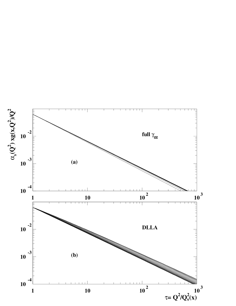
Figure 6: The solution $\alpha_{s}(Q^{2})xg(x,Q^{2})/Q_{s}^{2}(x)$ in the running coupling case. Rapidity range from $Y_{min}=6.0$ to $Y_{max}=46.0$ in steps $\Delta Y=2$. Upper plot (a): case with full anomalous dimension $\gamma_{gg}(\omega)$, lower plot: (b): case in DLLA approximation.

We consider now the case in which $\alpha_{s}$ is running and study the impact of scaling boundary condition (9) onto the evolution. We consider full expression for the anomalous dimension in that case $\gamma_{gg}(\omega)$ given by Eq.(44). The running of the coupling requires that the evolution is taken in the region well above the Landau pole. In our case this means that one has to evolve with $Q^{2}>Q_{s}^{2}(x)$ and we would like to have $Q_{s}^{2}(x)$ big enough for all values of $x$. For the purpose of illustration we take that $Q_{s}^{2}(x)=Q_{0}^{2}(x/x_{0})^{-\lambda}$ where $Q_{0}^{2}=1.0\;\rm GeV^{2}$ and $x_{0}=1.0$. This means that at $x=1$ the saturation scale is equal $Q_{s}^{2}=1.0\;\rm GeV^{2}$. This assumption might seem artificial considering the present phenomenology of lepton-nucleon scattering which suggests that saturation scale could be of the order of $1\;\rm GeV^{2}$ at $x\simeq 10^{-4}$ for the most central collisions at HERA collider [22, 28]. However, we use it here for the purpose of illustration of basic effects of the evolution with special scaling boundary conditions. We concentrate ourselves here on presenting general properties of the solution rather than trying to describe the experimental data. We also take $N_{f}=0$, that is we are considering pure gluonic channel. In Fig.6a we present the results of the calculation by plotting $\alpha_{s}(Q^{2})xg(x,Q^{2})/Q^{2}$ versus scaling variable $\tau=Q^{2}/Q_{s}^{2}(x)$ in the case with full gluon anomalous dimension. For comparison we also show the calculation performed in the DLLA approximation Fig. 6b. We see that the geometric scaling is mildly violated in the running coupling case, more strongly in the DLLA approximation due to the faster evolution. This fact can be understood on the basis of Eq.(41) where the numerical value of the exponent of expression on the r.h.s. is much bigger in the DLLA case: $b\gamma_{gg}(\lambda=0.5)=0.18$ in the case with full anomalous dimension and $b\gamma_{gg}(\lambda=0.5)=13/11$ in DLLA case.

We have tried to estimate whether the violation is consistent with the analytical prediction of formula (40). In Fig. 7a we present the same quantity as in Fig. 6a but multiplied by the scaling variable $\tau=Q^{2}/Q_{s}^{2}(x)$. The solid black curves in Fig. 7a from the upper to lower are for decreasing values of $x$. One can see that the solution exhibits some small violation of the geometric scaling and that the magnitude of this violation is smaller for smaller values of $x$ ( the curves are becoming closer and closer as $x$ decreases ). This is consistent with general behaviour predicted by equation (40) where the scaling violating factor on the r.h.s. tends to unity when $\ln(1/x)\gg 1$. We stress that the observed scaling violation is very small in this kinematical regime. For example at very high value of $\tau=10^{3}$ the violation of the scaling is about $5\%$ in a huge rapidity range from $Y=6$ to $Y=46$.

It follows from equations (40) and (41) that the violation of the geometric scaling can be approximately factored out. We checked this approximate prediction by considering the quantity

$$\alpha_{s}(Q^{2})xg(x,Q^{2})/Q_{s}^{2}(x)\,VF(x)$$

$${\rm with} VF(x)=\left[\frac{\ln(Q^{2}/Q_{s}^{2}(x))}{\ln(Q_{0}^{2}/\Lambda^{2})+\lambda\ln(1/x)}+1\right]^{1-b\gamma_{gg}(\lambda)}$$ (48)

which according to equation (40) should be constant with respect to $\tau=Q^{2}/Q_{s}^{2}(x)$. The results for the above quantity are shown in Fig. 7b (which is Fig. 7a multiplied by $VF(x)$ ) where now we see that approximately the geometric scaling is nearly restored (curves form a very narrow band) at high values of rapidity .

Also in the case of running coupling we have studied the features of the geometric scaling using the method of the derivative, see Eq. (46). The results are shown in Fig.8 where it is clear that there is always a region where the geometric scaling is (approximately) preserved in the running coupling case, even at very high values of $\tau$. This is consistent with formula (41) provided we have ${\bar{\alpha}_{s}}(Q_{s}^{2})\ln\tau\ll 1,\;x\ll 1$ and also with the conclusions of ref. [27, 29]. We have also illustrated in Fig.8 the sensitivity of the results on the variation of the normalisation for the saturation scale i.e. $Q_{0}^{2}$. Changing the parameter $Q_{0}^{2}$ from $1$ - upper plot in Fig.8 to $0.1\;\;{\rm GeV^{2}}$ - lower plot in Fig.8, influences the size of the violation of the scaling. One can see that the geometric scaling is postponed to the higher values of rapidity.

4 Summary and conclusions

In this paper we studied effects of the DGLAP evolution upon the geometric scaling. We solved the DGLAP evolution equation for the gluon distribution with the initial condition respecting the geometric scaling and provided along the critical line $Q^{2}=Q_{s}^{2}(x)$. In the case of the fixed QCD coupling we obtained analytic solution of the DGLAP equation with those boundary condition, Eq. (21). We also showed that for sufficiently large values of the parameter $\lambda$ defining the critical line this solution of the DGLAP equation preserves the geometric scaling for the leading term at small $x$, (see Eq. (22)). In the double logarithmic approximation of the DGLAP equation this happens for $\lambda\geq 4\bar{\alpha}_{s}$, where $\bar{\alpha}_{s}$ is defined by equation (27). Geometric scaling is however violated by effects which are subleading at small values of $x$. We have also obtained approximate solution of the DGLAP equation with the running coupling starting again from the boundary conditions respecting geometric scaling along the critical line. In the running coupling case geometric scaling is mildly violated for arbitrary values of the parameter $\lambda$ yet this violation can be approximately factored out. The size of this small violation is controlled by the quantity ${\bar{\alpha}_{s}}(Q_{s}^{2})\ln Q^{2}/Q_{s}^{2}$. Thus in the region where $x\ll 1$ and $\ln Q^{2}/Q_{s}^{2}\ll\ln Q_{s}^{2}/\Lambda^{2}$ the geometric scaling in the running coupling case is preserved. Results of the detailed numerical analysis confirmed all those expectations.
We conclude that the geometric scaling is a very useful regularity following from the saturation model. We believe that it might be interesting to incorporate this ’DGLAP improved’ geometric scaling in the phenomenological analysis of the data.

Figure 1: Phase diagram in $(\ln 1/x,\ln Q/\Lambda)$ space. Thick line is a critical line $Q^{2}=Q_{s}^{2}(x)$ which divides the saturation - scaling regime (to the left) and the linear - DGLAP regime (to the right).

Figure 2: Function $xg(x,Q^{2})/Q^{2}$ in DLLA fixed coupling case plotted versus scaling variable $\tau=Q^{2}/Q_{s}^{2}(x)$ for different values of rapidities $Y=\ln 1/x$, from $Y_{min}=6.0$ to $Y_{max}=46.0$ (solid curves from lower to upper) in steps $\Delta Y=2$ . Dashed curve is the input distribution $\sim 1/\tau$.

Figure 3: Function $xg(x,Q^{2})/Q^{2}$ in DLLA fixed coupling case plotted versus scaling variable $\tau=Q^{2}/Q_{s}^{2}(x)$ for different values of rapidities $Y=\ln 1/x$. Solid curves - solutions, dashed curve - input distribution $\sim 1/\tau$. On upper plot (a): solid curves from lower to upper are for $Y$ rapidities ranging from $Y_{min}=6.0$ to $Y_{max}=46.0$ in steps $\Delta Y=2$. Lower plot (b): rapidities ranging from $Y_{min}=26.0$ to $Y_{max}=46.0$ in steps $\Delta Y=2$.

Figure 4: Fixed coupling case with complete gluon anomalous dimension $\gamma_{gg}(\omega)$. Function $xg(x,Q^{2})/Q^{2}$ plotted versus scaling variable $\tau=Q^{2}/Q_{s}^{2}(x)$ for different values of rapidities $Y=\ln 1/x$ from $Y_{min}=6.0$ to $Y_{max}=46.0$ in steps $\Delta Y=2$. Upper plot (a): scaling exponent $\lambda=0.5$, lower plot (b): scaling exponent $\lambda=0.3$ .

Figure 5: The derivative $\Delta(Y,\tau)$ from Eq.(46) as a function of rapidity $Y$ for various values of the scaling variable $\tau$. Upper plot - scaling exponent $\lambda=0.5$, lower plot - scaling exponent $\lambda=0.3$.

Figure 7: The solution $\alpha_{s}(Q^{2})xg(x,Q^{2})/Q_{s}^{2}(x)$ in the running coupling case. We have selected high rapidity range from $Y_{min}=18.0$ to $Y_{max}=46.0$ in steps $\Delta Y=2$. Upper plot (a): $\alpha_{s}(Q^{2})xg(x,Q^{2})/Q_{s}^{2}(x)$, lower plot (b): $\alpha_{s}(Q^{2})xg(x,Q^{2})/Q_{s}^{2}(x)VF(x)$ where the factor $VF(x)$ is a scaling violation factor defined in equation (48).

Figure 8: The derivative $\Delta(Y,\tau)$ defined in Eq.(46) as a function of rapidity $Y$ for different values of $\tau$ and different choices of normalisation $Q_{0}^{2}$. The scaling exponent $\lambda$ was set to be equal $\lambda=0.5$.

References

- [1] L. V. Gribov, E. M. Levin and M. G. Ryskin, Phys. Rep. 100 (1983) 1.
- [2] A. H. Mueller and J. Qiu, Nucl. Phys. B268 (1986) 427.
- [3] A.H. Mueller, Nucl. Phys. B415 (1994) 373; A. H. Mueller and B. Patel, Nucl. Phys. B425 (1994) 471; A. H. Mueller, Nucl. Phys. B437 (1995) 107.
- [4] A. H. Mueller, Nucl. Phys. B335 (1990) 115; Yu. A. Kovchegov, A. H. Mueller and S. Wallon, Nucl. Phys. B507 (1997) 367. A. H. Mueller, Eur. Phys. J. A1 (1998) 19; Nucl. Phys. A654 (1999) 370; Nucl. Phys. B558 (1999) 285.
- [5] J. C. Collins and J. Kwieciński, Nucl. Phys. B335 (1990) 89; J. Bartels, G. A. Schuler and J. Blümlein, Z. Phys. C50 (1991) 91; Nucl. Phys. Proc. Suppl. 18 C (1991) 147.
- [6] J. Bartels and E. M. Levin, Nucl. Phys. B387 (1992) 617.
- [7] J. Bartels, Phys. Lett. B298 (1993) 204; Z. Phys. C60 (1993) 471; Z. Phys. C62 (1994) 425; J. Bartels and M. Wüsthoff, Z. Phys. C66 (1995) 157; J. Bartels and C. Ewerz, JHEP 9909 (1999) 026.
- [8] L. McLerran and R. Venugopalan, Phys. Rev. D49 (1994) 2233; Phys. Rev. D49 (1994) 3352; Phys. Rev. D50 (1994) 2225; A. Kovner, L. McLerran and H. Weigert, Phys. Rev. D52 (1995) 6231, Phys. Rev. D52 (1995) 3809; R. Venugopalan, Acta Phys. Polon. B30 (1999) 3731; E. Iancu and L. McLerran, Phys. Lett. B510 (2001) 145; L. McLerran, hep-ph/0104285; E. Iancu, A. Leonidov and L. McLerran, Nucl. Phys. A692 (2001) 583; E. Ferreiro, E. Iancu, A. Leonidov and L. McLerran, hep-ph/0109115; A. Capella et al., Phys. Rev. D63 (2001) 054010.
- [9] G. P. Salam, Nucl. Phys. B449 (1995) 589; Nucl. Phys. B461 (1996) 512; Comput. Phys. Commun. 105 (1997) 62; A. H. Mueller and G. P. Salam, Nucl. Phys. B475 (1996) 293.
- [10] E. Gotsman, E. M. Levin and U. Maor, Nucl. Phys. B464 (1996) 251; Nucl. Phys. B493 (1997) 354; Phys. Lett. B245 (1998) 369; Eur. Phys. J. C5 (1998) 303; E. Gotsman, E. M. Levin, U. Maor and E. Naftali, Nucl. Phys. B539 (1999) 535; A. L. Ayala Filho, M. B. Gay Ducati and E. M. Levin, Nucl. Phys. B493 (1997) 305;Nucl. Phys. B551 (1998) 355; Eur. Phys. J. C8 (1999) 115.
- [11] Ia. Balitsky, Nucl. Phys. B463 (1996) 99; I. I. Balitsky, Phys. Rev. Lett. 81 (1998) 2024; Phys. Rev. D60 (1999) 014020; hep-ph/0101042 ; Phys. Lett. B518 (2001) 235.
- [12] Yu. V. Kovchegov, Phys. Rev. D60 (1999) 034008; Phys. Rev. D61 (2000) 074018.
- [13] J. Jalilian-Marian, A. Kovner, L. McLerran and H. Weigert, Phys. Rev. D55 (1997) 5414; J. Jalilian-Marian, A. Kovner and H. Weigert, Phys. Rev. D59 (1999) 014014; Phys. Rev. D59 (1999) 014015; Phys. Rev. D59 (1999) 034007; Erratum – ibid. D59 (1999) 099903; A. Kovner, J. Guilherme Milhano and H. Weigert, Phys. Rev. D62 (2000) 114005; H. Weigert, NORDITA-2000-34-HE, hep-ph/0004044.
- [14] M. A. Braun, Eur. Phys. J. C16 (2000) 337; hep-ph/0101070.
- [15] Yu. V. Kovchegov and L. McLerran, —it Phys. Rev. D60 (1999) 054025; Erratum – ibid. D62 (2000) 019901; Yu. V. Kovchegov and E. M. Levin, Nucl. Phys. B577 (2000) 221.
- [16] E. M. Levin and M. Lublinsky, Nucl. Phys. A696 (2001) 833; Eur. Phys. J. C22 (2002) 647.
- [17] M. Lublinsky, Eur. Phys. J. C21 (2001) 513.
- [18] N. Armesto and M. A. Braun, Eur. Phys. J. C20 (2001) 517; Eur. Phys. J. C22 (2001) 351.
- [19] E. M. Levin and K. Tuchin, Nucl. Phys. B537 (2000) 833; Nucl. Phys. A691 (2001) 779; ibid. A693 (2001) 787.
- [20] K. Golec-Biernat, L. Motyka and A.M. Staśto, Phys. Rev. D65 (2002) 074037.
- [21] N. N. Nikolaev and B. G. Zakharov, Z. Phys. C49 (1991) 607; Z. Phys. C53 (1992) 331; Z. Phys. C64 (1994) 651; JETP 78 (1994) 598.
- [22] K. Golec-Biernat and M. Wüsthoff, Phys. Rev. D59 (1998) 014017; D60 (1999) 114023; Eur. Phys. J. C20 (2001) 313.
- [23] J. Bartels, K. Golec-Biernat and H. Kowalski, hep-ph/0203258.
- [24] S. Munier, hep-ph/0205319.
- [25] J.R. Forshaw, G.Kerley, G. Shaw, Phys. Rev. D60(1999) 074012; hep-ph/007257 .
- [26] A.M. Staśto, K. Golec-Biernat and J. Kwieciński, Phys. Rev. Lett. 86 (2001) 56.
- [27] E. Iancu, K. Itakura and L. McLerran, hep-ph/0203137.
- [28] S. Munier, A.M. Staśto, A.H. Mueller, Nucl. Phys. B603 (2001) 427.
- [29] A.H. Mueller, D.N. Triantafyllopoulos, hep-ph/0205167.