Supergraph Techniques and Two-Loop Beta-Functions for Renormalizable and Non-Renormalizable Operators

Abstract:

We present a construction kit for calculating two-loop beta functions in $N\!=\!1$ supersymmetric theories for the operators of the superpotential using supergraph techniques. In particular, it allows to compute the beta functions for every desired, even higher dimensional, operator of the superpotential from the wavefunction renormalization constants of the theory. We apply this method to calculate the two-loop beta functions for the lowest-dimensional effective neutrino mass operator in the Minimal Supersymmetric Standard Model (MSSM) and for the Yukawa couplings in the MSSM extended by singlet superfields and the mass matrix for the latter. Our method can be applied to any $N\!=\!1$ supersymmetric theory.

1 Introduction

In order to compare experimental results with predictions from models beyond the Standard Model (SM), like unified theories, it is essential to evolve the parameters of the models from high to low energies. This is accomplished with the renormalization group equations (RGE’s) for the operators in the theory. Besides the renormalizable operators there can be higher dimensional, non-renormalizable operators if the theory is considered as effective.

In a previous study [1], we derived a general method for calculating $\beta$-functions from counterterms in MS-like renormalization schemes, which works for tensorial quantities. It is simplified considerably in supersymmetric (SUSY) theories, since due to the non-renormalization theorem [2, 3] only wavefunction renormalization has to be considered for operators of the superpotential. However, in a component field description, no use can be made of the theorem with respect to gauge loop corrections since it is no longer manifest when a supergauge, as for example Wess-Zumino-gauge, has been fixed. The supergraph technique [4, 5, 6, 7], on the other hand, allows to use the non-renormalization theorem, since SUSY is kept manifest. Moreover, it has the advantage that the number of independent diagrams is clearly reduced compared to the component field calculations.

We therefore present a method to calculate $\beta$-functions in supersymmetric theories for operators of the superpotential from wavefunction renormalization. These operators may be non-renormalizable since for the latter the non-renormalization theorem holds as well [8], and they do not affect the wavefunction renormalization constants in leading order in an effective field theory expansion. As an application, we consider the Minimal Supersymmetric Standard Model (MSSM) extended by singlet superfields, which contain right-handed neutrinos relevant for models of neutrino mass. We compute and specify the wavefunction renormalization constants. From these, the two loop RGE’s for the Yukawa couplings and for a possible mass matrix for the singlet neutrino superfields are obtained by the supergraph method. The technique can be used to compute the two loop RGE’s for every desired higher dimensional operator of the superpotential, since the non-renormalization theorem guarantees that no vertex corrections contribute. Furthermore, we consider the lowest dimensional neutrino mass operator. Its RGE is known at the one loop level for the SM [9, 10, 1], Two Higgs Doublet Models [10, 11] and for the MSSM [9, 10, 11]. With the supergraph method we calculate the two loop RGE for the neutrino mass operator from the MSSM wavefunction renormalization constants.

2 Review of the Supergraph Method

Consider a general supersymmetric gauge theory with a gauge part described by the usual Lagrangian

$$\mathscr{L} = \int\mathrm{d}^{4}\theta\,\sum_{i,j=1}^{N}\overline{\bbPhi}^{(i)}\,\left[\exp(2g\cdot\mathbb{V})\right]_{ij}\,{}^{(j)}+\left[\frac{1}{4}\int\mathrm{d}^{2}\theta\,\sum_{n=1}^{S}\mathbb{W}_{\alpha}^{n}\mathbb{W}^{n\,\alpha}+\text{h.c.}\right]$$ (1)

$$+\left[\int\mathrm{d}^{2}\theta\,\mathscr{W}+\text{h.c.}\right]+\mathscr{L}_{\mathrm{Ghost}}+\mathscr{L}_{\mathrm{Gauge\>Fixing}}$$

where

$$\mathbb{W}_{\alpha}^{n} = \frac{1}{8g_{n}}\,\overline{\boldsymbol{D}}^{2}\left[\exp(2g_{n}\,\mathbb{V}^{n})\,\boldsymbol{D}_{\alpha}\,\exp(-2g_{n}\mathbb{V}^{n})\right]\;,$$ (2a)

$$g\cdot\mathbb{V} := \sum_{n=1}^{S}g_{n}\,\mathbb{V}^{n}\quad\text{and}\quad\mathbb{V}^{n}=\sum_{A=1}^{\dim G_{n}}\mathbb{V}_{n}^{A}\,\mathsf{T}_{n}^{A}\;.$$ (2b)

The renormalizable part of the superpotential reads

$$\mathscr{W}_{\mathrm{ren}}=\frac{1}{6}\sum_{i,j,k=1}^{N}\lambda_{(ijk)}\,{}^{(i)}\,{}^{(j)}\,{}^{(k)}\;.$$ (3)

Possible mass terms are ignored for the present as they do not affect the $\beta$-functions of the model. The $N$ superfields ⁽ⁱ⁾ transform under the irreducible representations (irreps) $R^{(i)}_{1}\times\cdots\times R^{(i)}_{S}$ of the gauge group $G_{1}\otimes\cdots\otimes G_{S}$. $\{(\mathsf{T}_{n}^{A})_{i}^{j}\}_{A=1}^{\dim G_{n}}$ denote the generators of $G_{n}$. The indices $i,j,\dots$ run over all irreps, families and the representation space.

2.1 Wavefunction Renormalization Constants

Due to the non-renormalization theorem, the RGE’s for operators of the superpotential are governed by the wavefunction renormalization constants for the superfields ${Z}_{ij}=\mathbbm{1}_{ij}+\delta Z_{ij}$ which relate the bare ${}^{(i)}_{\mathrm{B}}$ and the renormalized superfields,

$${}^{(i)}_{\mathrm{B}}=\sum_{j=1}^{N}Z_{ij}^{\frac{1}{2}}{}^{(j)}\;.$$ (4)

Results are obtained with dimensional regularization via dimensional reduction [12, 13]. At the one loop level and in $d=4-\epsilon$ dimensions, $\delta Z_{ij}$ is given by

$$-\delta Z_{ij}^{(1)}=\frac{1}{(4\pi)^{2}}\frac{1}{\epsilon}\,\left[\sum_{k,\ell=1}^{N}\lambda_{ik\ell}^{*}\lambda_{jk\ell}-4\sum_{n=1}^{S}g_{n}^{2}\,c_{2}\left(R^{(i)}_{n}\right)\,\delta_{ij}\right]\;.$$ (5)

In equation (5) and in the following, we use the group-theoretical constants

$$c_{1}(G)\,\delta^{AB} := \sum_{C,D}f^{ACD}f^{B}{}_{CD}\;,$$ (6a)

$$c_{2}(R)\,\delta_{ab} := \sum_{A}(\mathsf{T}^{A}\mathsf{T}^{A})_{ab}\;,$$ (6b)

$$\ell(R)\,\delta^{AB} := \text{Tr}(\mathsf{T}^{A}\mathsf{T}^{B})\;,$$ (6c)

with the matrix representations $\{\mathsf{T}^{A}\}_{A=1}^{\dim G}$ of the generators of $G$ corresponding to the irrep $R$ and the structure constants $f^{A}{}_{BC}$. $\ell(R)$ is known as Dynkin index of the irrep $R$ and $c_{2}(R)$ as the quadratic Casimir. They are related by

$$c_{2}(R)=\frac{\dim G}{\dim R}\,\ell(R)\;,$$ (7)

with $\dim G$ and $\dim R$ being the dimension of the group $G$ and the irrep $R$, respectively. Often the generators of the irrep $\boldsymbol{N}$ of $\mathrm{SU}(N)$ are normalized such that $\ell(\boldsymbol{N})=\frac{1}{2}$ holds. $c_{2}$ can then be obtained via $c_{2}(\boldsymbol{N})=\frac{N^{2}-1}{2N}$ while for a $\mathrm{U}(1)$ theory both $\ell(R)$ and $c_{2}(R)$ are replaced by $q^{2}$ where $q$ is the $\mathrm{U}(1)$ charge of . For any non-trivial irrep of $\text{SU}(N)$ the invariant $c_{1}(\boldsymbol{N})$ is given by $N$.

On the two-loop level the renormalization group equations are determined from the formula [14]

$$-\delta Z_{ij}^{(2)} = \frac{-2+\epsilon}{(4\pi)^{4}\,\epsilon^{2}}\,\left[4\sum_{n,m=1}^{S}g_{n}^{2}\,c_{2}\!\left(R^{(i)}_{n}\right)\,g_{m}^{2}\,c_{2}\!\left(R^{(j)}_{m}\right)\,\delta_{ij}\right.$$ (8)

$$\hphantom{\frac{-2+\epsilon}{(4\pi)^{4}\,\epsilon^{2}}\,\left[\right.}+2\,\sum_{n=1}^{S}g_{n}^{4}\,c_{2}\!\left(R^{(i)}_{n}\right)\,\left(\overline{\ell}_{n}-3\,c_{1}(G_{n})\right)\,\delta_{ij}$$

$$\hphantom{\frac{-2+\epsilon}{(4\pi)^{4}\,\epsilon^{2}}\,\left[\right.}+\sum_{n=1}^{S}\sum_{k,\ell=1}^{N}g_{n}^{2}\left(-\,c_{2}\!\left(R^{(i)}_{n}\right)+2\,c_{2}\!\left(R^{(\ell)}_{n}\right)\right)\,\lambda_{ik\ell}^{*}\lambda_{jk\ell}$$

$$\left.\hphantom{\frac{-2+\epsilon}{(4\pi)^{4}\,\epsilon^{2}}\,\left[\right.}-\frac{1}{2}\sum_{k,\ell,r,s,t=1}^{N}\lambda_{ik\ell}^{*}\lambda_{\ell st}\,\lambda_{rst}^{*}\lambda_{jkr}\right]\;.$$

Here $\overline{\ell}_{n}$ is defined by

$$\overline{\ell}_{n}:=\sum_{i=1}^{N}\frac{\ell\left(R_{n}^{(i)}\right)}{\dim\left(R_{n}^{(i)}\right)}\;.$$ (9)

In addition to the superpotential of equation (3), higher dimensional operators may appear in the superpotential of an effective theory. These operators are generally suppressed by inverse powers of a large mass scale $M_{X}$. Though these operators are non-renormalizable by power counting, in the effective field theory approach one can renormalize the theory in an expansion in inverse powers of $M_{X}$. In the leading order of this expansion, the higher dimensional operators do not contribute to the wavefunction renormalization.

In supergraphs, we represent chiral superfields as straight double lines while vector-superfields are indicated by wiggly double lines,

$$\begin{array}[]{rcl}\bbPhi\hfil&:&\vbox{\hbox{\includegraphics{SuperGraph12.eps}}}\;,\\ \mathbb{V}&:&\vbox{\hbox{\includegraphics{SuperGraph13.eps}}}\;.\end{array}$$

The diagrams relevant for the calculation of the wavefunction renormalization constants for the matter superfield, equation (5) and (8), are shown in figure 1 and 2, respectively.

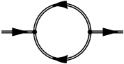
(a)

(b)

Figure 1: One-loop supergraphs which contribute to the $\overline{\bbPhi}\bbPhi$ propagator.

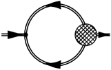
(a)

(b)

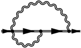
(c)

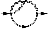
(d)

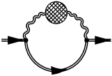
(e)

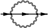
(f)

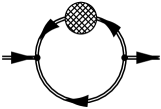
(g)

(h)

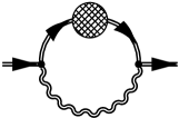
(i)

Figure 2: Two-loop supergraphs which contribute to the $\overline{\bbPhi}\bbPhi$ propagator. A blob denotes the relevant one-particle irreducible graph including any one-loop counterterm that may be required [14].

2.2 $\beta$-Functions from Wavefunction Renormalization Constants

To calculate $\beta$-functions from the wavefunction renormalization constants, it is convenient to subdivide the general indices $\{i,j,\dots\}$ into indices $\{r,s,\dots\}$ for the irreducible representations, $\{f,g,\dots\}$ for the particle families and $\{a,b,\dots\}$ for the representation space, i.e. $i=(r,f,a)$. The wavefunction renormalization constants $Z_{ij}$ are diagonal with respect to the representation and the representation space indices and are matrices in flavour-space. In the rest of the paper we will write $Z_{ij}=Z_{r}$ and suppress flavour and representation space indices.

Due to the non-renormalization theorem, in a supersymmetric theory a bare quantity $Q_{\mathrm{B}}$ of the superpotential and the corresponding renormalized one, $Q$, are related by

$$Q_{\mathrm{B}}=\left(\prod\limits_{r\in I}Z_{r}^{n_{r}}\right)\,Q\,\mu^{D_{Q}\epsilon}\,\left(\prod\limits_{s\in J}Z_{s}^{n_{s}}\right)\;,$$ (10)

where matrix multiplication with respect to flavour indices is implicit and the sets of superfield indices $I=\{1,\dots M\}$ and $J=\{M+1,\dots N\}$ denote the wavefunction renormalization constants multiplied from the left and the right respectively. $Q$ may correspond to a renormalizable or non-renormalizable operator.

The wavefunction renormalization constants $Z_{r}$ can be expanded in $\epsilon$,

$$Z_{r}=1+\sum_{k\geq 1}\frac{Z_{r,k}}{\epsilon^{k}}\;.$$ (11)

Following the steps of the derivation in [1], we find

$$\beta_{Q} = Q\cdot\sum_{s\in J}n_{s}\left[\sum_{A}D_{V_{A}}\,\Braket{\frac{\mathrm{d}Z_{s,1}}{\mathrm{d}V_{A}}}{V_{A}}\right]$$ (12)

$$\hphantom{Q\cdot\sum_{s\in J}n_{s}\left[\right.}+\sum_{r\in I}n_{r}\left[\sum_{A}D_{V_{A}}\,\Braket{\frac{\mathrm{d}Z_{r,1}}{\mathrm{d}V_{A}}}{V_{A}}\right]\cdot Q\;,$$

where $\{V_{A}\}$ denotes the set of all variables of the theory including the variable $Q$ under consideration and $\beta_{Q}$ is the usual $\beta$-function, defined by

$$\beta_{Q}=\mu\frac{\mathrm{d}Q}{\mathrm{d}\mu}\;.$$ (13)

Note that in equation (12), for complex quantities $V_{A}$ we have to treat the complex conjugates $V^{*}_{A}$ as independent variables. We use the notation [1]

$$\Braket{\frac{\mathrm{d}F}{\mathrm{d}x}}{y}:=\left\{\begin{array}[]{ll}\displaystyle\frac{\mathrm{d}F}{\mathrm{d}x}y&\text{for scalars}\;x,y\\ \displaystyle\sum_{n}\frac{\mathrm{d}F}{\mathrm{d}x_{n}}y_{n}&\text{for vectors}\;x=(x_{m}),y=(y_{m})\\ \displaystyle\sum_{m,n}\frac{\mathrm{d}F}{\mathrm{d}x_{mn}}y_{mn}&\text{for matrices}\;x=(x_{mn}),y=(y_{mn})\\ \dots&\text{etc.}\end{array}\right.$$ (18)

and $D_{V_{A}}$ is related to the mass dimension of $V_{A}$ as indicated in equation (10). Equation (12) allows to compute the $\beta$-functions directly from the wavefunction renormalization constants, calculated with the supergraph technique. It has a form that can easily be used for computer algebra calculations.

3 Applications

3.1 Two-Loop $\beta$-Functions in the MSSM Extended by Singlet Superfields

We consider a supersymmetric model containing the same fields as the MSSM and additionally the singlet “neutrino” superfield which we will denote by . In order to obtain the $\beta$-functions for the Yukawa matrices and a mass matrix for the neutrino superfield, we will omit the soft SUSY breaking terms, since they do not affect the considered $\beta$-functions above the scale of the soft supersymmetry breaking mass terms. Threshold effects at low energy scales are e.g. discussed in [19].

Thus the Yukawa part of the superpotential is given by

$$\mathscr{W}_{\mathrm{Yukawa}} = (Y_{e})_{gf}\mathbb{e}^{\mathrm{C}g}\mathbb{h}^{(1)}_{a}\varepsilon^{ab}\mathbb{l}^{f}_{b}+(Y_{\nu})_{gf}{}^{\mathrm{C}g}\mathbb{h}^{(2)}_{a}\varepsilon^{ab}\mathbb{l}^{f}_{b}$$ (19)

$$+(Y_{d})_{gf}\mathbb{d}^{\mathrm{C}g}\mathbb{h}^{(1)}_{a}\varepsilon^{ab}\mathbb{q}^{f}_{b}+(Y_{u})_{gf}\mathbb{u}^{\mathrm{C}g}\mathbb{h}^{(2)}_{a}(\varepsilon^{T})^{ab}\mathbb{q}_{b}^{f}\;.$$

The superfields $\mathbb{e}^{\mathrm{C}}$, $\mathbb{d}^{\mathrm{C}}$ and $\mathbb{u}^{\mathrm{C}}$ contain the $\mathrm{SU}(2)_{\mathrm{L}}$-singlet charged leptons, down-type quarks and up-type quarks, respectively, and $\mathbb{q}$ contains the SU(2)_L quark doublets. Their quantum numbers are specified in table LABEL:tab:QuantumNumbersOfNuMSSM. In addition we consider a mass term for the singlet neutrino superfield

$$\mathscr{W}_{\mathrm{Mass}}=\tfrac{1}{2}\,{}^{\mathrm{C}\,f}M_{fg}{}^{\mathrm{C}\,g}\;,$$ (20)

that may be relevant for generating neutrino masses in the see-saw scenario.

The quantum numbers of the superfields are listed in table LABEL:tab:QuantumNumbersOfNuMSSM. Note that we use GUT charge normalization for the $\mathrm{U}(1)_{\mathrm{Y}}$ charge.

Field	$\mathbb{h}^{(1)}$	$\mathbb{h}^{(2)}$	$\mathbb{q}$	${\mathbb{d}}^{\mathrm{C}}$	${\mathbb{u}}^{\mathrm{C}}$	$\mathbb{l}$	${\mathbb{e}}^{\mathrm{C}}$	C
$\vphantom{\bigg{|}}\sqrt{\frac{5}{3}}q_{\mathrm{Y}}$	$-\tfrac{1}{2}$	$+\tfrac{1}{2}$	$+\tfrac{1}{6}$	$+\tfrac{1}{3}$	$-\tfrac{2}{3}$	$-\tfrac{1}{2}$	$+1$	$0$
$\vphantom{\big{|}}\mathrm{SU}(2)_{\mathrm{L}}$	$\boldsymbol{2}$	$\boldsymbol{2}$	$\boldsymbol{2}$	$\boldsymbol{1}$	$\boldsymbol{1}$	$\boldsymbol{2}$	$\boldsymbol{1}$	$\boldsymbol{1}$
$\vphantom{\big{|}}\mathrm{SU}(3)_{\mathrm{C}}$	$\boldsymbol{1}$	$\boldsymbol{1}$	$\boldsymbol{3}$	$\overline{\boldsymbol{3}}$	$\overline{\boldsymbol{3}}$	$\boldsymbol{1}$	$\boldsymbol{1}$	$\boldsymbol{1}$

Table 1: Quantum numbers of the superfields. $q_{\mathrm{Y}}$ denotes the $\mathrm{U}(1)_{\mathrm{Y}}$ charge in GUT normalization.

Using equation (5), this leads to the $1/\epsilon$-coefficients of the wavefunction renormalization constants

$$-(4\pi)^{2}\,Z_{\mathbb{h}^{(1)},1}^{(1)} = 6\,\text{Tr}(Y_{d}^{\dagger}\cdot Y_{d})+2\,\text{Tr}(Y_{e}^{\dagger}\cdot Y_{e})-\frac{3}{5}\,g_{1}^{2}-3\,g_{2}^{2}\;,$$ (21a)

$$-(4\pi)^{2}\,Z_{\mathbb{h}^{(2)},1}^{(1)} = 6\,\text{Tr}(Y_{u}^{\dagger}\cdot Y_{u})+2\,\text{Tr}(Y_{\nu}^{\dagger}\cdot Y_{\nu})-\frac{3}{5}\,g_{1}^{2}-3\,g_{2}^{2}\;,$$ (21b)

$$-(4\pi)^{2}\,Z_{\mathbb{q},1}^{(1)} = 2\,Y_{d}^{\dagger}\cdot Y_{d}+2\,Y_{u}^{\dagger}\cdot Y_{u}-\frac{1}{15}\,g_{1}^{2}-3\,g_{2}^{2}-\frac{16}{3}\,g_{3}^{2}\;,$$ (21c)

$$-(4\pi)^{2}\,Z_{\mathbb{d}^{\mathrm{C}},1}^{(1)} = 4\,Y_{d}^{*}\cdot Y_{d}^{T}-\frac{4}{15}\,g_{1}^{2}-\frac{16}{3}\,g_{3}^{2}\;,$$ (21d)

$$-(4\pi)^{2}\,Z_{\mathbb{u}^{\mathrm{C}},1}^{(1)} = 4\,Y_{u}^{*}\cdot Y_{u}^{T}-\frac{16}{15}\,g_{1}^{2}-\frac{16}{3}\,g_{3}^{2}\;,$$ (21e)

$$-(4\pi)^{2}\,Z_{\mathbb{l},1}^{(1)} = 2\,Y_{e}^{\dagger}\cdot Y_{e}+2\,Y_{\nu}^{\dagger}\cdot Y_{\nu}-\frac{3}{5}\,g_{1}^{2}-3\,g_{2}^{2}\;,$$ (21f)

$$-(4\pi)^{2}\,Z_{\mathbb{e}^{\mathrm{C}},1}^{(1)} = 4\,Y_{e}^{*}\cdot Y_{e}^{T}-\frac{12}{5}\,g_{1}^{2}\;,$$ (21g)

$$-(4\pi)^{2}\,Z_{{}^{\mathrm{C}},1}^{(1)} = 4\,Y_{\nu}^{*}\cdot Y_{\nu}^{T}\;,$$ (21h)

where the $Y$’s as well as the last six $Z$-factors are of course matrices in flavour space. From the two-loop diagrams we get

$$-(4\pi)^{4}\,\frac{Z_{\mathbb{h}^{(1)},1}^{(2)}}{2} = -9\,\text{Tr}(Y_{d}\cdot Y_{d}^{\dagger}\cdot Y_{d}\cdot Y_{d}^{\dagger})-3\,\text{Tr}(Y_{u}\cdot Y_{d}^{\dagger}\cdot Y_{d}\cdot Y_{u}^{\dagger})$$ (22a)

$$-3\,\text{Tr}(Y_{e}\cdot Y_{e}^{\dagger}\cdot Y_{e}\cdot Y_{e}^{\dagger})-\text{Tr}(Y_{e}\cdot Y_{\nu}^{\dagger}\cdot Y_{\nu}\cdot Y_{e}^{\dagger})$$

$$-\frac{2}{5}\,g_{1}^{2}\,\text{Tr}(Y_{d}^{\dagger}\cdot Y_{d})+\frac{6}{5}\,g_{1}^{2}\,\text{Tr}(Y_{e}^{\dagger}\cdot Y_{e})+16\,g_{3}^{2}\,\text{Tr}(Y_{d}^{\dagger}\cdot Y_{d})$$

$$+\frac{207}{100}\,g_{1}^{4}+\frac{9}{10}\,g_{1}^{2}\,g_{2}^{2}+\frac{15}{4}\,g_{2}^{4}\;,$$

$$-(4\pi)^{4}\,\frac{Z_{\mathbb{h}^{(2)},1}^{(2)}}{2} = -3\,\text{Tr}(Y_{u}\cdot Y_{d}^{\dagger}\cdot Y_{d}\cdot Y_{u}^{\dagger})-9\,\text{Tr}(Y_{u}\cdot Y_{u}^{\dagger}\cdot Y_{u}\cdot Y_{u}^{\dagger})$$ (22b)

$$-\text{Tr}(Y_{\nu}\cdot Y_{e}^{\dagger}\cdot Y_{e}\cdot Y_{\nu}^{\dagger})-3\,\text{Tr}(Y_{\nu}\cdot Y_{\nu}^{\dagger}\cdot Y_{\nu}\cdot Y_{\nu}^{\dagger})$$

$$+\frac{4}{5}\,g_{1}^{2}\,\text{Tr}(Y_{u}^{\dagger}\cdot Y_{u})+16\,g_{3}^{2}\,\text{Tr}(Y_{u}^{\dagger}\cdot Y_{u})$$

$$+\frac{207}{100}\,g_{1}^{4}+\frac{9}{10}\,g_{1}^{2}\,g_{2}^{2}+\frac{15}{4}\,g_{2}^{4}\;,$$

$$-(4\pi)^{4}\,\frac{Z_{\mathbb{q},1}^{(2)}}{2} = -2\,Y_{d}^{\dagger}\cdot Y_{d}\cdot Y_{d}^{\dagger}\cdot Y_{d}-2\,Y_{u}^{\dagger}\cdot Y_{u}\cdot Y_{u}^{\dagger}\cdot Y_{u}$$ (22c)

$$-3\,Y_{d}^{\dagger}\cdot Y_{d}\,\text{Tr}(Y_{d}\cdot Y_{d}^{\dagger})-3\,Y_{u}^{\dagger}\cdot Y_{u}\,\text{Tr}(Y_{u}\cdot Y_{u}^{\dagger})$$

$$-Y_{d}^{\dagger}\cdot Y_{d}\,\text{Tr}(Y_{e}\cdot Y_{e}^{\dagger})-Y_{u}^{\dagger}\cdot Y_{u}\,\text{Tr}(Y_{\nu}\cdot Y_{\nu}^{\dagger})$$

$$+\frac{2}{5}\,g_{1}^{2}\,Y_{d}^{\dagger}\cdot Y_{d}+\frac{4}{5}\,g_{1}^{2}\,Y_{u}^{\dagger}\cdot Y_{u}$$

$$+\frac{199}{900}\,g_{1}^{4}+\frac{1}{10}\,g_{1}^{2}\,g_{2}^{2}+\frac{15}{4}\,g_{2}^{4}$$

$$+\frac{8}{45}\,g_{1}^{2}\,g_{3}^{2}+8\,g_{2}^{2}\,g_{3}^{2}-\frac{8}{9}\,g_{3}^{4}\;,$$

$$-(4\pi)^{4}\,\frac{Z_{\mathbb{d}^{\mathrm{C}},1}^{(2)}}{2} = -2\,Y_{d}^{*}\cdot Y_{d}^{T}\cdot Y_{d}^{*}\cdot Y_{d}^{T}-2\,Y_{d}^{*}\cdot Y_{u}^{T}\cdot Y_{u}^{*}\cdot Y_{d}^{T}$$ (22d)

$$-6\,Y_{d}^{*}\cdot Y_{d}^{T}\,\text{Tr}(Y_{d}\cdot Y_{d}^{\dagger})-2\,Y_{d}^{*}\cdot Y_{d}^{T}\,\text{Tr}(Y_{e}\cdot Y_{e}^{\dagger})$$

$$+\frac{2}{5}\,g_{1}^{2}\,Y_{d}^{*}\cdot Y_{d}^{T}+6\,g_{2}^{2}\,Y_{d}^{*}\cdot Y_{d}^{T}$$

$$+\frac{202}{225}\,g_{1}^{4}+\frac{32}{45}\,g_{1}^{2}\,g_{3}^{2}-\frac{8}{9}\,g_{3}^{4}\;,$$

$$-(4\pi)^{4}\,\frac{Z_{\mathbb{u}^{\mathrm{C}},1}^{(2)}}{2} = -2\,Y_{u}^{*}\cdot Y_{d}^{T}\cdot Y_{d}^{*}\cdot Y_{u}^{T}-2\,Y_{u}^{*}\cdot Y_{u}^{T}\cdot Y_{u}^{*}\cdot Y_{u}^{T}$$ (22e)

$$-2\,Y_{u}^{*}\cdot Y_{u}^{T}\,\text{Tr}(Y_{\nu}\cdot Y_{\nu}^{\dagger})-6\,Y_{u}^{*}\cdot Y_{u}^{T}\,\text{Tr}(Y_{u}\cdot Y_{u}^{\dagger})$$

$$-\frac{2}{5}\,g_{1}^{2}\,Y_{u}^{*}\cdot Y_{u}^{T}+6\,g_{2}^{2}\,Y_{u}^{*}\cdot Y_{u}^{T}$$

$$+\frac{856}{225}\,g_{1}^{4}+\frac{128}{45}\,g_{1}^{2}\,g_{3}^{2}-\frac{8}{9}\,g_{3}^{4}\;,$$

$$-(4\pi)^{4}\,\frac{Z_{\mathbb{l},1}^{(2)}}{2} = -2\,Y_{e}^{\dagger}\cdot Y_{e}\cdot Y_{e}^{\dagger}\cdot Y_{e}-2\,Y_{\nu}^{\dagger}\cdot Y_{\nu}\cdot Y_{\nu}^{\dagger}\cdot Y_{\nu}$$ (22f)

$$-3\,Y_{e}^{\dagger}\cdot Y_{e}\,\text{Tr}(Y_{d}\cdot Y_{d}^{\dagger})-Y_{e}^{\dagger}\cdot Y_{e}\,\text{Tr}(Y_{e}\cdot Y_{e}^{\dagger})$$

$$-3\,Y_{\nu}^{\dagger}\cdot Y_{\nu}\,\text{Tr}(Y_{u}\cdot Y_{u}^{\dagger})-Y_{\nu}^{\dagger}\cdot Y_{\nu}\,\text{Tr}(Y_{\nu}\cdot Y_{\nu}^{\dagger})$$

$$+\frac{6}{5}\,g_{1}^{2}\,Y_{e}^{\dagger}\cdot Y_{e}+\frac{207}{100}\,g_{1}^{4}+\frac{9}{10}\,g_{1}^{2}\,g_{2}^{2}+\frac{15}{4}\,g_{2}^{4}\;,$$

$$-(4\pi)^{4}\,\frac{Z_{\mathbb{e}^{\mathrm{C}},1}^{(2)}}{2} = -2\,Y_{e}^{*}\cdot Y_{e}^{T}\cdot Y_{e}^{*}\cdot Y_{e}^{T}-2\,Y_{e}^{*}\cdot Y_{\nu}^{T}\cdot Y_{\nu}^{*}\cdot Y_{e}^{T}$$ (22g)

$$-6\,Y_{e}^{*}\cdot Y_{e}^{T}\,\text{Tr}(Y_{d}\cdot Y_{d}^{\dagger})-2\,Y_{e}^{*}\cdot Y_{e}^{T}\,\text{Tr}(Y_{e}\cdot Y_{e}^{\dagger})$$

$$-\frac{6}{5}\,g_{1}^{2}\,Y_{e}^{*}\cdot Y_{e}^{T}+6\,g_{2}^{2}\,Y_{e}^{*}\cdot Y_{e}^{T}+\frac{234}{25}\,g_{1}^{4}\;,$$

$$-(4\pi)^{4}\,\frac{Z_{{}^{\mathrm{C}},1}^{(2)}}{2} = -2\,Y_{\nu}^{*}\cdot Y_{e}^{T}\cdot Y_{e}^{*}\cdot Y_{\nu}^{T}-2\,Y_{\nu}^{*}\cdot Y_{\nu}^{T}\cdot Y_{\nu}^{*}\cdot Y_{\nu}^{T}$$ (22h)

$$-6\,Y_{\nu}^{*}\cdot Y_{\nu}^{T}\,\text{Tr}(Y_{u}\cdot Y_{u}^{\dagger})-2\,Y_{\nu}^{*}\cdot Y_{\nu}^{T}\,\text{Tr}(Y_{\nu}\cdot Y_{\nu}^{\dagger})$$

$$+\frac{6}{5}\,g_{1}^{2}\,Y_{\nu}^{*}\cdot Y_{\nu}^{T}+6\,g_{2}^{2}\,Y_{\nu}^{*}\cdot Y_{\nu}^{T}\;,$$

respectively. From these, the two-loop Yukawa RGE’s are derived,

$$\mu\frac{\mathrm{d}Y_{x}}{\mathrm{d}\mu}=\frac{1}{(4\pi)^{2}}\beta_{Y_{x}}^{(1)}+\frac{1}{(4\pi)^{4}}\beta_{Y_{x}}^{(2)}\;,$$ (23)

where $x\in\{d,u,e,\nu\}$. Using equation (12), the one-loop contributions to the $\beta$-functions are given by

$$\beta_{Y_{d}}^{(1)} = Y_{d}\cdot\left\{\vphantom{\frac{1}{2}}\right.3\,Y_{d}^{\dagger}\cdot Y_{d}+Y_{u}^{\dagger}\cdot Y_{u}+3\,\text{Tr}(Y_{d}^{\dagger}\cdot Y_{d})+\text{Tr}(Y_{e}^{\dagger}\cdot Y_{e})$$ (24a)

$$\hphantom{Y_{d}\cdot\left\{\right.}{}-\frac{7}{15}\,g_{1}^{2}-3\,g_{2}^{2}-\frac{16}{3}\,g_{3}^{2}\left.\vphantom{\frac{1}{2}}\right\}\;,$$

$$\beta_{Y_{u}}^{(1)} = Y_{u}\cdot\left\{\vphantom{\frac{1}{2}}\right.Y_{d}^{\dagger}\cdot Y_{d}+3\,Y_{u}^{\dagger}\cdot Y_{u}+\text{Tr}(Y_{\nu}^{\dagger}\cdot Y_{\nu})+3\,\text{Tr}(Y_{u}^{\dagger}\cdot Y_{u})$$ (24b)

$$\hphantom{Y_{u}\cdot\left\{\right.}{}-\frac{13}{15}\,g_{1}^{2}-3\,g_{2}^{2}-\frac{16}{3}\,g_{3}^{2}\left.\vphantom{\frac{1}{2}}\right\}\;$$

$$\beta_{Y_{e}}^{(1)} = Y_{e}\cdot\left\{\vphantom{\frac{1}{2}}\right.3\,Y_{e}^{\dagger}\cdot Y_{e}+Y_{\nu}^{\dagger}\cdot Y_{\nu}+3\,\text{Tr}(Y_{d}^{\dagger}\cdot Y_{d})+\text{Tr}(Y_{e}^{\dagger}\cdot Y_{e})$$ (24c)

$$\hphantom{Y_{e}\cdot\left\{\right.}{}-\frac{9}{5}\,g_{1}^{2}-3\,g_{2}^{2}\left.\vphantom{\frac{1}{2}}\right\}\;,$$

$$\beta_{Y_{\nu}}^{(1)} = Y_{\nu}\cdot\left\{\vphantom{\frac{1}{2}}\right.Y_{e}^{\dagger}\cdot Y_{e}+3\,Y_{\nu}^{\dagger}\cdot Y_{\nu}+3\,\text{Tr}(Y_{u}^{\dagger}\cdot Y_{u})+\text{Tr}(Y_{\nu}^{\dagger}\cdot Y_{\nu})$$ (24d)

$$\hphantom{Y_{\nu}\cdot\left\{\right.}{}-\frac{3}{5}\,g_{1}^{2}-3\,g_{2}^{2}\left.\vphantom{\frac{1}{2}}\right\}\;,$$

and the two-loop contributions are

$$\beta_{Y_{d}}^{(2)} = Y_{d}\cdot\left\{\vphantom{\frac{1}{2}}-4\,Y_{d}^{\dagger}\cdot Y_{d}\cdot Y_{d}^{\dagger}\cdot Y_{d}-2\,Y_{u}^{\dagger}\cdot Y_{u}\cdot Y_{d}^{\dagger}\cdot Y_{d}-2\,Y_{u}^{\dagger}\cdot Y_{u}\cdot Y_{u}^{\dagger}\cdot Y_{u}\right.$$ (25a)

$$\hphantom{Y_{d}\cdot\left\{\right.}{}-9\,\text{Tr}(Y_{d}\cdot Y_{d}^{\dagger}\cdot Y_{d}\cdot Y_{d}^{\dagger})-3\,\text{Tr}(Y_{d}\cdot Y_{u}^{\dagger}\cdot Y_{u}\cdot Y_{d}^{\dagger})$$

$$\hphantom{Y_{d}\cdot\left\{\right.}{}-3\,\text{Tr}(Y_{e}\cdot Y_{e}^{\dagger}\cdot Y_{e}\cdot Y_{e}^{\dagger})-\text{Tr}(Y_{e}\cdot Y_{\nu}^{\dagger}\cdot Y_{\nu}\cdot Y_{e}^{\dagger})$$

$$\hphantom{Y_{d}\cdot\left\{\right.}{}-9\,Y_{d}^{\dagger}\cdot Y_{d}\,\text{Tr}(Y_{d}\cdot Y_{d}^{\dagger})-3\,Y_{d}^{\dagger}\cdot Y_{d}\,\text{Tr}(Y_{e}\cdot Y_{e}^{\dagger})$$

$$\hphantom{Y_{d}\cdot\left\{\right.}{}-Y_{u}^{\dagger}\cdot Y_{u}\,\text{Tr}(Y_{\nu}\cdot Y_{\nu}^{\dagger})-3\,Y_{u}^{\dagger}\cdot Y_{u}\,\text{Tr}(Y_{u}\cdot Y_{u}^{\dagger})$$

$$\hphantom{Y_{d}\cdot\left\{\right.}{}+6\,g_{2}^{2}\,Y_{d}^{\dagger}\cdot Y_{d}+\frac{4}{5}\,g_{1}^{2}\,Y_{d}^{\dagger}\cdot Y_{d}+\frac{4}{5}\,g_{1}^{2}\,Y_{u}^{\dagger}\cdot Y_{u}$$

$$\hphantom{Y_{d}\cdot\left\{\right.}{}-\frac{2}{5}\,g_{1}^{2}\,\text{Tr}(Y_{d}^{\dagger}\cdot Y_{d})+\frac{6}{5}\,g_{1}^{2}\,\text{Tr}(Y_{e}^{\dagger}\cdot Y_{e})+16\,g_{3}^{2}\,\text{Tr}(Y_{d}^{\dagger}\cdot Y_{d})$$

$$\hphantom{Y_{d}\cdot\left\{\right.}{}+\frac{287}{90}\,g_{1}^{4}+g_{1}^{2}\,g_{2}^{2}+\frac{15}{2}\,g_{2}^{4}+\frac{8}{9}\,g_{1}^{2}\,g_{3}^{2}+8\,g_{2}^{2}\,g_{3}^{2}-\frac{16}{9}\,g_{3}^{4}\left.\vphantom{\frac{1}{2}}\right\}\;,$$

$$\beta_{Y_{u}}^{(2)} = Y_{u}\cdot\left\{-2\,Y_{d}^{\dagger}\cdot Y_{d}\cdot Y_{d}^{\dagger}\cdot Y_{d}-2\,Y_{d}^{\dagger}\cdot Y_{d}\cdot Y_{u}^{\dagger}\cdot Y_{u}-4\,Y_{u}^{\dagger}\cdot Y_{u}\cdot Y_{u}^{\dagger}\cdot Y_{u}\right.$$ (25b)

$$\hphantom{Y_{u}\cdot\left\{\right.}{}-3\,Y_{d}^{\dagger}\cdot Y_{d}\,\text{Tr}(Y_{d}\cdot Y_{d}^{\dagger})-Y_{d}^{\dagger}\cdot Y_{d}\,\text{Tr}(Y_{e}\cdot Y_{e}^{\dagger})$$

$$\hphantom{Y_{u}\cdot\left\{\right.}{}-9\,Y_{u}^{\dagger}\cdot Y_{u}\,\text{Tr}(Y_{u}\cdot Y_{u}^{\dagger})-3\,Y_{u}^{\dagger}\cdot Y_{u}\,\text{Tr}(Y_{\nu}\cdot Y_{\nu}^{\dagger})$$

$$\hphantom{Y_{u}\cdot\left\{\right.}{}-3\,\text{Tr}(Y_{u}\cdot Y_{d}^{\dagger}\cdot Y_{d}\cdot Y_{u}^{\dagger})-9\,\text{Tr}(Y_{u}\cdot Y_{u}^{\dagger}\cdot Y_{u}\cdot Y_{u}^{\dagger})$$

$$\hphantom{Y_{u}\cdot\left\{\right.}{}-\text{Tr}(Y_{\nu}\cdot Y_{e}^{\dagger}\cdot Y_{e}\cdot Y_{\nu}^{\dagger})-3\,\text{Tr}(Y_{\nu}\cdot Y_{\nu}^{\dagger}\cdot Y_{\nu}\cdot Y_{\nu}^{\dagger})$$

$$\hphantom{Y_{u}\cdot\left\{\right.}{}+\frac{2}{5}\,g_{1}^{2}\,Y_{d}^{\dagger}\cdot Y_{d}+\frac{2}{5}\,g_{1}^{2}\,Y_{u}^{\dagger}\cdot Y_{u}+6\,g_{2}^{2}\,Y_{u}^{\dagger}\cdot Y_{u}$$

$$\hphantom{Y_{u}\cdot\left\{\right.}{}+\frac{4}{5}\,g_{1}^{2}\,\text{Tr}(Y_{u}^{\dagger}\cdot Y_{u})+16\,g_{3}^{2}\,\text{Tr}(Y_{u}^{\dagger}\cdot Y_{u})+\frac{2743}{450}\,g_{1}^{4}$$

$$\hphantom{Y_{u}\cdot\left\{\right.}{}+g_{1}^{2}\,g_{2}^{2}+\frac{15}{2}\,g_{2}^{4}+\frac{136}{45}\,g_{1}^{2}\,g_{3}^{2}+8\,g_{2}^{2}\,g_{3}^{2}-\frac{16}{9}\,g_{3}^{4}\left.\vphantom{\frac{1}{2}}\right\}\;,$$

$$\beta_{Y_{e}}^{(2)} = Y_{e}\cdot\left\{\vphantom{\frac{1}{2}}\right.-4\,Y_{e}^{\dagger}\cdot Y_{e}\cdot Y_{e}^{\dagger}\cdot Y_{e}-2\,Y_{\nu}^{\dagger}\cdot Y_{\nu}\cdot Y_{e}^{\dagger}\cdot Y_{e}-2\,Y_{\nu}^{\dagger}\cdot Y_{\nu}\cdot Y_{\nu}^{\dagger}\cdot Y_{\nu}$$ (25c)

$$\hphantom{Y_{e}\cdot\left\{\right.}{}-9\,Y_{e}^{\dagger}\cdot Y_{e}\,\text{Tr}(Y_{d}\cdot Y_{d}^{\dagger})-3\,Y_{e}^{\dagger}\cdot Y_{e}\,\text{Tr}(Y_{e}\cdot Y_{e}^{\dagger})$$

$$\hphantom{Y_{e}\cdot\left\{\right.}{}-Y_{\nu}^{\dagger}\cdot Y_{\nu}\,\text{Tr}(Y_{\nu}\cdot Y_{\nu}^{\dagger})-3\,Y_{\nu}^{\dagger}\cdot Y_{\nu}\,\text{Tr}(Y_{u}\cdot Y_{u}^{\dagger})$$

$$\hphantom{Y_{e}\cdot\left\{\right.}{}-9\,\text{Tr}(Y_{d}\cdot Y_{d}^{\dagger}\cdot Y_{d}\cdot Y_{d}^{\dagger})-3\,\text{Tr}(Y_{d}\cdot Y_{u}^{\dagger}\cdot Y_{u}\cdot Y_{d}^{\dagger})$$

$$\hphantom{Y_{e}\cdot\left\{\right.}{}-3\,\text{Tr}(Y_{e}\cdot Y_{e}^{\dagger}\cdot Y_{e}\cdot Y_{e}^{\dagger})-\text{Tr}(Y_{e}\cdot Y_{\nu}^{\dagger}\cdot Y_{\nu}\cdot Y_{e}^{\dagger})+\frac{6}{5}\,g_{1}^{2}\,\text{Tr}(Y_{e}^{\dagger}\cdot Y_{e})$$

$$\hphantom{Y_{e}\cdot\left\{\right.}{}+6\,g_{2}^{2}\,Y_{e}^{\dagger}\cdot Y_{e}-\frac{2}{5}\,g_{1}^{2}\,\text{Tr}(Y_{d}^{\dagger}\cdot Y_{d})+16\,g_{3}^{2}\,\text{Tr}(Y_{d}^{\dagger}\cdot Y_{d})$$

$$\hphantom{Y_{e}\cdot\left\{\right.}{}+\frac{27}{2}\,g_{1}^{4}+\frac{9}{5}\,g_{1}^{2}\,g_{2}^{2}+\frac{15}{2}\,g_{2}^{4}\left.\vphantom{\frac{1}{2}}\right\}\;,$$

$$\beta_{Y_{\nu}}^{(2)} = Y_{\nu}\cdot\left\{\vphantom{\frac{1}{2}}\right.-2\,Y_{e}^{\dagger}\cdot Y_{e}\cdot Y_{e}^{\dagger}\cdot Y_{e}-2\,Y_{e}^{\dagger}\cdot Y_{e}\cdot Y_{\nu}^{\dagger}\cdot Y_{\nu}-4\,Y_{\nu}^{\dagger}\cdot Y_{\nu}\cdot Y_{\nu}^{\dagger}\cdot Y_{\nu}$$ (25d)

$$\hphantom{Y_{\nu}\cdot\left\{\right.}{}-3\,Y_{e}^{\dagger}\cdot Y_{e}\,\text{Tr}(Y_{d}\cdot Y_{d}^{\dagger})-Y_{e}^{\dagger}\cdot Y_{e}\,\text{Tr}(Y_{e}\cdot Y_{e}^{\dagger})$$

$$\hphantom{Y_{\nu}\cdot\left\{\right.}-3\,Y_{\nu}^{\dagger}\cdot Y_{\nu}\,\text{Tr}(Y_{\nu}\cdot Y_{\nu}^{\dagger})-9\,Y_{\nu}^{\dagger}\cdot Y_{\nu}\,\text{Tr}(Y_{u}\cdot Y_{u}^{\dagger})$$

$$\hphantom{Y_{\nu}\cdot\left\{\right.}{}-\text{Tr}(Y_{\nu}\cdot Y_{e}^{\dagger}\cdot Y_{e}\cdot Y_{\nu}^{\dagger})-3\,\text{Tr}(Y_{\nu}^{\dagger}\cdot Y_{\nu}\cdot Y_{\nu}^{\dagger}\cdot Y_{\nu})$$

$$\hphantom{Y_{\nu}\cdot\left\{\right.}{}-3\,\text{Tr}(Y_{u}\cdot Y_{d}^{\dagger}\cdot Y_{d}\cdot Y_{u}^{\dagger})-9\,\text{Tr}(Y_{u}\cdot Y_{u}^{\dagger}\cdot Y_{u}\cdot Y_{u}^{\dagger})$$

$$\hphantom{Y_{\nu}\cdot\left\{\right.}{}+\frac{6}{5}\,g_{1}^{2}\,Y_{e}^{\dagger}\cdot Y_{e}+\frac{6}{5}\,g_{1}^{2}\,Y_{\nu}^{\dagger}\cdot Y_{\nu}+6\,g_{2}^{2}\,Y_{\nu}^{\dagger}\cdot Y_{\nu}$$

$$\hphantom{Y_{\nu}\cdot\left\{\right.}{}+\frac{4}{5}\,g_{1}^{2}\,\text{Tr}(Y_{u}^{\dagger}\cdot Y_{u})+16\,g_{3}^{2}\,\text{Tr}(Y_{u}^{\dagger}\cdot Y_{u})$$

$$\hphantom{Y_{\nu}\cdot\left\{\right.}{}+\frac{207}{50}\,g_{1}^{4}+\frac{9}{5}\,g_{1}^{2}\,g_{2}^{2}+\frac{15}{2}\,g_{2}^{4}\left.\vphantom{\frac{1}{2}}\right\}\;.$$

Note that the two-loop MSSM RGE’s for $Y_{d}$, $Y_{u}$ and $Y_{e}$ are easily obtained by setting $Y_{\nu}=0$. The effort is clearly reduced compared to component field calculations [20, 21, 22].

3.2 Two-Loop $\beta$-Function for the Effective Neutrino Mass Operator

We now apply our method to calculate the $\beta$-function for the lowest dimensional effective neutrino mass operator, which is contained in the $F$-term of the superpotential

$$\mathscr{W}_{\kappa}^{\mathrm{MSSM}}=-\frac{1}{4}{\kappa}_{gf}\,\mathbb{l}^{g}_{c}\varepsilon^{cd}\mathbb{h}^{(2)}_{d}\,\,\mathbb{l}_{b}^{f}\varepsilon^{ba}\mathbb{h}^{(2)}_{a}+\text{h.c.}\;.$$ (26)

It can e.g. be obtained by integrating out the singlet superfield of the model described in section 3.1 at leading order in the effective theory. The $\beta$-function can easily be computed using our method. Substituting $D_{g_{i}}=D_{Y_{x}}=\frac{1}{2}$ with $i\in\{1,2,3\}$ and $x\in\{u,d,e\}$, we get from equation (12)

$$\beta_{\kappa}=-Z_{\mathbb{h}^{(2)},1}\cdot\kappa-\frac{1}{2}\,Z_{\mathbb{l},1}^{T}\cdot\kappa-\frac{1}{2}\,\kappa\cdot Z_{\mathbb{l},1}\;.$$ (27)

We can thus write the $\beta$-function for $\kappa$ in the form

$$\beta_{\kappa}=X^{T}\cdot\kappa+\kappa\cdot X+\alpha\,\kappa\;,$$ (28)

where the complete flavour diagonal part is contained in $\alpha$. We further split $X=X^{(1)}+X^{(2)}$ and $\alpha=\alpha^{(1)}+\alpha^{(2)}$ into their one loop and two loop part. Plugging in the wavefunction renormalization constants of equation (21b) and (21f) and setting $Y_{\nu}=0$, our method reproduces the one loop results of [9, 10, 11]

$$(4\pi)^{2}\,X^{(1)} = Y_{e}^{\dagger}\cdot Y_{e}\;,$$ (29a)

$$(4\pi)^{2}\,\alpha^{(1)} = -\frac{6}{5}\,g_{1}^{2}-6\,g_{2}^{2}+6\,\text{Tr}(Y_{u}^{\dagger}\cdot Y_{u})\;.$$ (29b)

Note that for $\mathrm{U}(1)_{\mathrm{Y}}$, we use GUT charge normalization as specified in table LABEL:tab:QuantumNumbersOfNuMSSM. At two-loop, with the wavefunction renormalization constants given in equations (22b) and (22f), we obtain

$$(4\pi)^{4}\,X^{(2)} = -2\,Y_{e}^{\dagger}\cdot Y_{e}\cdot Y_{e}^{\dagger}\cdot Y_{e}$$ (30)

$${}+\left(\frac{6}{5}\,g_{1}^{2}-\text{Tr}(Y_{e}\cdot Y_{e}^{\dagger})-3\,\text{Tr}(Y_{d}\cdot Y_{d}^{\dagger})\right)\,Y_{e}^{\dagger}\cdot Y_{e}$$

and

$$(4\pi)^{4}\,\alpha^{(2)} = -6\,\text{Tr}(Y_{u}\cdot Y_{d}^{\dagger}\cdot Y_{d}\cdot Y_{u}^{\dagger})-18\,\text{Tr}(Y_{u}\cdot Y_{u}^{\dagger}\cdot Y_{u}\cdot Y_{u}^{\dagger})$$ (31)

$${}+\frac{8}{5}\,g_{1}^{2}\,\text{Tr}(Y_{u}^{\dagger}\cdot Y_{u})+32\,g_{3}^{2}\,\text{Tr}(Y_{u}^{\dagger}\cdot Y_{u})$$

$${}+\frac{207}{25}\,\,g_{1}^{4}+\frac{18}{5}\,g_{1}^{2}\,g_{2}^{2}+15\,g_{2}^{4}\;.$$

3.3 Two-Loop $\beta$-Function for the Mass of the Singlet Superfield

From the wavefunction renormalization constants of the MSSM extended by singlet superfields given in section 3.1, the $\beta$-function for the bilinear coupling of equation (20) can easily be computed using the formula of equation (12). At one-loop, we find

$$(4\pi)^{2}\beta_{M}^{(1)}=2\,M\cdot Y_{\nu}^{*}\cdot Y_{\nu}^{T}+2\,Y_{\nu}\cdot Y_{\nu}^{\dagger}\cdot M$$ (32)

and the two-loop part of the $\beta$-function is given by

$$(4\pi)^{4}\beta_{M}^{(2)} = M\cdot\left[\vphantom{\frac{1}{2}}\right.-2\,Y_{\nu}^{*}\cdot Y_{e}^{T}\cdot Y_{e}^{*}\cdot Y_{\nu}^{T}-2\,Y_{\nu}^{*}\cdot Y_{\nu}^{T}\cdot Y_{\nu}^{*}\cdot Y_{\nu}^{T}$$ (33)

$$\hphantom{M\cdot\left[\right.}{}-6\,Y_{\nu}^{*}\cdot Y_{\nu}^{T}\,\text{Tr}(Y_{u}\cdot Y_{u}^{\dagger})-2\,Y_{\nu}^{*}\cdot Y_{\nu}^{T}\,\text{Tr}(Y_{\nu}\cdot Y_{\nu}^{\dagger})$$

$$\hphantom{M\cdot\left[\right.}{}+\frac{6}{5}\,g_{1}^{2}\,Y_{\nu}^{*}\cdot Y_{\nu}^{T}+6\,g_{2}^{2}\,Y_{\nu}^{*}\cdot Y_{\nu}^{T}\left.\vphantom{\frac{1}{2}}\right]$$

$${}+\left[\vphantom{\frac{1}{2}}\right.-2\,Y_{\nu}\cdot Y_{e}^{\dagger}\cdot Y_{e}\cdot Y_{\nu}^{\dagger}-2\,Y_{\nu}\cdot Y_{\nu}^{\dagger}\cdot Y_{\nu}\cdot Y_{\nu}^{\dagger}$$

$$\hphantom{+\left[\right.}{}-6\,Y_{\nu}\cdot Y_{\nu}^{\dagger}\,\text{Tr}(Y_{u}\cdot Y_{u}^{\dagger})-2\,Y_{\nu}\cdot Y_{\nu}^{\dagger}\,\text{Tr}(Y_{\nu}\cdot Y_{\nu}^{\dagger})$$

$$\hphantom{+\left[\right.}{}+\frac{6}{5}\,g_{1}^{2}\,Y_{\nu}\cdot Y_{\nu}^{\dagger}+6\,g_{2}^{2}\,Y_{\nu}\cdot Y_{\nu}^{\dagger}\left.\vphantom{\frac{1}{2}}\right]\cdot M\;.$$

In typical models of neutrino masses based on the see-saw mechanism, the effective neutrino mass operator of equation (26) is obtained by integrating out the singlet superfields, which leads to the relation $\kappa=2Y_{\nu}^{T}M^{-1}Y_{\nu}$. The $\beta$-function for $M$, together with the $\beta$-function for $Y_{\nu}$ of equation (24d), is therefore required to evolve the neutrino mass matrix from the GUT scale to the scale of the largest eigenvalue of $M$, if the singlets have a direct mass term.

4 Discussion and Conclusions

We have presented a general method to calculate two loop $\beta$-functions for renormalizable and non-renormalizable operators of the superpotential using superfield techniques. This method is very useful for model building since it provides a construction kit which allows to calculate the $\beta$-functions in a given supersymmetric GUT model with little effort. We have applied this method to calculate the two-loop beta functions for the lowest-dimensional effective neutrino mass operator in the MSSM and for the the Yukawa couplings and the mass matrix in the MSSM extended by singlet chiral superfields. We have computed and specified the wavefunction renormalization constants in the latter model, from which, using our method, the two loop RGE’s for every, even higher dimensional, operator of the superpotential can directly be computed. A classification of several higher-dimensional operators for generating neutrino Majorana masses is e.g. given in [23]. Many of them can be generalized for supersymmetric models. Their $\beta$-functions can easily be obtained with our method. The two loop $\beta$-function for the lowest-dimensional effective neutrino mass operator is required to increase the accuracy of many studies based on the one loop RGE [9, 10, 11], e.g. [24, 25, 26, 27, 28, 29, 30, 31, 32]. This accuracy may be needed for the neutrino sector since due to the absence of hadronic uncertainties, high precision measurements of the neutrino parameters may be achieved in future experiments.