Sweeping the Space of
Admissible Quark Mass Matrices

Abstract

We propose a new and efficient method of reconstructing quark mass matrices from their eigenvalues and a complete set of mixing observables. By a combination of the principle of NNI bases which are known to cover the general case, and of the polar decomposition theorem that allows to convert arbitrary nonsingular matrices to triangular form, we achieve a parameterization where the remaining freedom is reduced to one complex parameter. While this parameter runs through the domain bounded by the circle with radius $R=\sqrt{(m_{t}^{2}-m_{u}^{2})/(m_{t}^{2}-m_{c}^{2})}$ around the origin in the complex plane one sweeps the space of all mass matrices compatible with the given set of data.

PACS: 12.15Ff, 12.15Hh
Keywords: Quark mass matrices, Flavor mixing

I Introduction

The four three-generation mass sectors of quarks and leptons belong to the deepest enigmas of the standard model of strong and electroweak interactions. While there is a great amount of experimental information of steadily increasing accuracy, theoretical models of mass matrices and mixing matrices are scarce. In this unsatisfactory situation it seems of utmost importance to parameterize the available data in such a way that possible textures in the mass matrices of a given charge sector become visible in an unambiguous manner. For instance, in the case of quarks, there are 10 data, viz. the masses of the three charge $+2/3$ quarks, the masses of the three charge $-1/3$ quarks, and four observables in the Cabibbo-Kobayashi-Maskawa (CKM) matrix, to be compared to 12 physically significant parameters in the mass matrices $M^{(u)}$ and $M^{(d)}$. Therefore, reconstructing mass matrices from the data really amounts to finding an optimal parameterization that exhibits the remaining two-parameter freedom in a transparent way.

An important step in this direction was taken by Branco et al. who realized that the class of so-called nearest-neighbour-interaction (NNI)-bases for chiral states are economical but still completely general [4], and may hence be used in attempts to reconstruct the mass matrices from the observed mass eigenvalues and the empirical mixing matrices. These authors also gave an explicit procedure for constructing mass matrices in an NNI basis, for arbitrary mass sectors of quarks. Unfortunately, their analysis involves solving cubic equations. Although soluble in principle, these equations are too cumbersome to solve and do not allow for a practical and efficient reconstruction.

In this paper we propose a new method of reconstruction that avoids these shortcomings. We conjecture that this method and the appropriate parameterization are optimal in the sense of concentrating the remaining freedom in a single complex parameter whose domain of variation can be restricted to the interior of a circle in the complex plane. In particular, we succeed in reconstructing the mass matrices proper, up to unobservable changes of basis. This goes beyond, say, the work of Harayama and Okamura [5] who express the CKM matrix in terms of six parameters, with a two-parameter freedom. The way from their result to the mass matrices seems involved and not well suited for a practical analysis.

We make use of the polar decomposition theorem for nonsingular matrices [6]

$$M\,=\,T\,W\;\,,$$

where $T$ is a lower-triangular matrix and $W$ is a unitary matrix which, when applying this formula to three generations of chiral quarks, can be absorbed in the right-chiral fields. If, in addition, we work in the class of NNI bases in which the $(21)$-element of $T$ is seen to vanish, we still cover the most general case but get rid of all redundant quantities. More precisely, if

$$\widehat{H}^{(q)}=M^{(q)}M^{(q)\dagger}=\widehat{T}^{(q)}\widehat{T}^{(q)\dagger}\,,\qquad q=u,d\,,$$

are the “squared” hermitean mass matrices and $D^{(q)}=\mbox{diag }\bigl{(}m_{1}^{2},m_{2}^{2},m_{3}^{2}\bigr{)}$ with $m_{1}\equiv m_{u}$ or $m_{d}$ etc. their diagonal forms, then, in any NNI basis,

$$\widehat{H}^{(u)}=U^{\dagger}D^{(u)}U\,,\;\;\widehat{H}^{(d)}=U^{\dagger}V_{\rm CKM}D^{(d)}V_{\rm CKM}^{\dagger}U\,.$$

The matrix $U$ which is known analytically [7], depends on two complex parameters, say $a$ and $b$ defined in eq. (54) below. These parameters are related through a quadratic equation whose coefficients are elements of the matrix

$$V_{\rm CKM}D^{(d)}V_{\rm CKM}^{\dagger}\,,$$

i.e. of a matrix that is obtained solely from experimental data! Solving for one or the other of them, say $b=b(a)$, reduces the set of admissible mass matrices to the expected two-parameter freedom in the variable $a$. Progress achieved in this way is twofold: On the one hand, parameterization in terms of, say, $a$ is analytically simple and transparent. On the other hand, the domain of variation of $a$ and the formulae for the elements of $\widehat{H}^{(u)}$ and $\widehat{H}^{(d)}$ are such that the space of admissible mass matrices can be studied graphically and numerically, as $a$ sweeps through all allowed values, in a quantitatively reliable manner. Although we have not done this yet, one can even follow the propagation of the error bars of the experimental input, in not too involved a procedure.

The paper is organised as follows: In sect. 2 we review the choice of NNI bases and recapitulate the relevance of the polar decomposition theorem for the problem at stake. Sect. 3 which is the main body of our work, describes the explicit construction of the matrix $U$ as well as its parameterization in terms of $a$, $b$, and the squared masses of the up-sector. The NNI condition is encoded in the quadratic equation (64) below. In sect. 4 we discuss symmetries helpful in solving that constraint, and consider some limiting cases in order to illustrate the method. We also propose an expansion of the solutions in terms of a parameter which, due to the hierarchy in the quark masses, is numerically very small. The final sect. 5 gives two examples of how a conjectured texture of mass matrices can be checked against the data in a simple and transparent manner, by converting the mass matrices to the (general) form studied here. It ends with a few conclusions.

II General nearest-neighbour bases and triangular matrices

In the case of three generations the mass matrices $\widehat{M}^{(u)}$ and $\widehat{M}^{(d)}$ in the so called nearest neighbour interaction (NNI) basis are characterized by the following generic structure,

$$\widehat{M}^{(u)},\;\widehat{M}^{(d)}\;=\;\left(\begin{array}[]{ccc}0&\star&0\\ \star&0&\star\\ 0&\star&\star\end{array}\right)\;\;\;.$$ (1)

Here the “$\star$”-entries appearing on the r.h.s. of (1) are arbitrary non-vanishing, complex numbers. The interpretation of this particular choice of the mass matrices that is usually given by its proponents is the following: the $(11)$- and $(22)$-elements are put equal to zero, while letting the $(33)$-element be different from zero, with the idea of describing an initial, no-interaction situation where two quarks are massless and only one is massive. Furthermore, only neighbouring generations are allowed to interact, by assuming nonvanishing $(12)$-, $(21)$-, $(23)$-, and $(32)$-elements, but vanishing $(13)$- and $(31)$-elements.

However, it has been known for a long time that this setting, although very tempting and intuitive at first sight, is ill-defined unless it is supplemented by further assumptions. Indeed, Branco, Lavoura, and Mota showed in [4] that any set of admissible mass matrices $\{M^{(u)},M^{(d)}\}$ of the standard model, i.e. any set of two completely arbitrary non-singular $3\times 3$-matrices, can be transformed to the form given in (1) without the need for any further assumption. In other words, in the framework of the minimal standard model where only left-chiral fermion fields participate in charged current weak interactions, the mass matrices in (1) are still completely general, the specific form (1) reflecting no more than a specific choice of chiral basis. This fact is mainly due to the observation that weak interactions of quarks remain unchanged under the simultaneous transformations

$$M^{(u)} \rightarrow \widehat{M}^{(u)}\;=\;U^{\dagger}M^{(u)}V_{u}\;\;\;\mbox{ and}$$ (2)

$$M^{(d)} \rightarrow \widehat{M}^{(d)}\;=\;U^{\dagger}M^{(d)}V_{d}\;\;\;,$$ (3)

of the mass matrices, where $U,V_{u}$ and $V_{d}$ are arbitrary unitary $3\times 3$-matrices: On the one hand, the unitaries $V_{u}$ and $V_{d}$ act on the right-chiral fields $(u_{R},c_{R},t_{R})$ and $(d_{R},s_{R},b_{R})$, respectively, and, hence, can be absorbed by a redefinition of these unobservable fields, without loss of generality. On the other hand, the common unitary matrix $U$ in (2) which acts on the left-chiral quark fields, drops out when calculating the physical Cabibbo-Kobayashi-Maskawa (CKM) matrix

$$V_{\rm CKM}\;=\;U^{(u)}_{L}U^{(d)\dagger}_{L}\;\;\;.$$ (4)

In (4) $U^{(u)}_{L}$ and $U^{(d)}_{L}$ are the unitary matrices which diagonalize the “squared”, hermitean mass matrices

$$H^{(q)}=M^{(q)}M^{(q)\dagger}\,,\qquad q=u,d\,,$$ (5)

of the up- and down-sector, respectively, viz.

$$U^{(u)}_{L}H^{(u)}U^{(u)\dagger}_{L} = \mbox{diag}(m_{u}^{2},m_{c}^{2},m_{t}^{2})\equiv D^{(u)}\;,$$ (6)

$$U^{(d)}_{L}H^{(d)}U^{(d)\dagger}_{L} = \mbox{diag}(m_{d}^{2},m_{s}^{2},m_{b}^{2})\equiv D^{(d)}\;.$$ (7)

Thus, as proved in [4], the structure (1) of the mass matrices corresponds to no more than a special, physically admissible choice of the electroweak basis. The interpretation sketched above fully rests on this choice and will no longer be valid in other electroweak bases. Unless this special choice is singled out by additional arguments that could stem, e.g., from physics beyond the standard model, the above interpretation loses its physical significance because physics, of course, must not depend on the choice of basis.
There is an alternative derivation of the same conclusion which, at the same time, helps us to fix notations for our subsequent calculations. As was shown in [7], [8], when dealing with questions of reconstructing mass matrices from the experimental data, i.e. from four independent absolute values of CKM matrix elements and the six quark masses, a most economic but nevertheless physically completely general parameterization of the quark mass matrices is given by triangular mass matrices,

$$T^{(u)},\;T^{(d)}=\left(\begin{array}[]{ccc}\star&0&0\\ \star&\star&0\\ \star&\star&\star\end{array}\right)\;\;\;.$$ (8)

This parameterization results upon exploiting the polar decomposition theorem for non-singular, but otherwise arbitrary matrices:

$$M^{(q)}\;=\;T^{(q)}W^{(q)}\;,\quad q=u,d\,,\quad\mbox{with }W^{(q)}\mbox{ unitary}.$$ (9)

Again, the unitaries $W^{(q)}$, $q=u,d$, can be absorbed by a redefinition of the right-chiral quark fields, without loss of generality.
At the level of the squared mass matrices $\widehat{H}^{(q)}$ the NNI structure (1) of the mass matrices is equivalent to a vanishing $(12)$-element (and – because $\widehat{H}^{(q)}$ is hermitean – also a vanishing $(21)$-element):

$$\widehat{H}^{(q)}_{12}\;=\;0\;=\;\widehat{H}^{(q)}_{21}\;\;,\;\;q=u,d\;.$$ (10)

Because of $\widehat{H}^{(q)}=\widehat{M}^{(q)}\widehat{M}^{(q)\dagger}=\widehat{T}^{(q)}\widehat{T}^{(q)\dagger}$, $q=u,d$, a straightforward calculation shows that within the triangular parameterization the NNI condition (10) reads

$$\widehat{T}^{(q)}_{21}\;=\;0\;,\qquad q=u,d\;\;\;.$$ (11)

Mimicking for a moment the (invalid) interpretation mentioned in connection with the NNI structure (1), eq. (11) would suggest that there is no direct interaction between the first and the second generation while, in the basis (1), these evidently do mix, and, in fact, mix strongly. Direct interactions seem to be present between the second and third generations as well as between the first and third generations only, due to the non-vanishing $(32)$- and $(31)$-elements of $\widehat{T}^{(q)}$, respectively, in contrast to (1) where seemingly there is no direct coupling between first and third generations.
These statements underpin once more that such an interpretation is dependent on the electroweak basis chosen for the representation of the mass matrices and, hence, should better be avoided altogether.

Although it is unrelated to a specific physical picture of quark masses and mixings, bases that yield the NNI form of the mass matrices turn out to be very useful in the process of reconstructing mass matrices from the observed quark mixings and masses. Therefore, in what follows we shall make extensive use of this class of bases. That is to say, we start from triangular mass matrices whose $(21)$-elements are zero, viz.

$$\widehat{T}^{(u)}=\left(\begin{array}[]{ccc}\hat{\alpha}&0&0\\ 0&\hat{\beta}&0\\ \hat{\kappa}_{3}e^{{\rm i}\hat{\varphi}_{3}}&\hat{\kappa}_{2}e^{{\rm i}\hat{\varphi}_{2}}&\hat{\gamma}\end{array}\right)\;\;\;,\;\;\;\widehat{T}^{(d)}=\left(\begin{array}[]{ccc}\hat{\alpha}^{\prime}&0&0\\ 0&\hat{\beta}^{\prime}&0\\ \hat{\kappa}^{\prime}_{3}e^{{\rm i}\hat{\varphi}^{\prime}_{3}}&\hat{\kappa}^{\prime}_{2}e^{{\rm i}\hat{\varphi}^{\prime}_{2}}&\hat{\gamma}^{\prime}\end{array}\right)\;.$$ (12)

Here and in the sequel the hat on the symbols refers to the choice of an NNI basis.

Possible phases can be absorbed into the right-chiral fields and, hence, without loss of generality, the matrix elements $\hat{\alpha},\hat{\beta},\hat{\gamma}$ and $\hat{\alpha}^{\prime},\hat{\beta}^{\prime},\hat{\gamma}^{\prime}$ along the diagonals may be chosen to be real. In fact, also the phases $\hat{\varphi}_{2}$ and $\hat{\varphi}_{3}$ could be dropped by making use of the unitary matrix $U$ in (2) thereby rendering $\widehat{T}^{(u)}$ real. In doing so, on the theoretical side we are left with 12 parameters, 5 from the up-sector and 7 from the down-sector. These have to be confronted with 10 experimental data, i.e. 6 quark masses + 4 real observables in the CKM matrix, leaving a freedom of two parameters. This is characteristic for an NNI basis.

III An efficient reconstruction procedure

The authors of [4] give a detailed prescription for the construction of mass matrices in an NNI basis, for arbitrary mass matrices: The main step consists in solving the eigenvalue problem

$$(H^{(u)}+\kappa H^{(d)})_{ij}\;u_{j2}\;=\;\lambda\;u_{i2}$$ (13)

for the matrix $H^{(u)}+\kappa H^{(d)}$, where $\kappa$ denotes an arbitrary complex number. Note that $\kappa$ reflects the two-parameter freedom within the class of NNI matrices. Once the second column $(u_{i2})$ of the unitary matrix $U$, which transforms the arbitrary squared mass matrices (5) to NNI form (see (2)) is determined according to (13), the first column $(u_{i1})$ is calculated by means of

$$u_{i1}\;\propto\;\epsilon_{ijk}\;u_{j2}^{\star}\;u_{l2}^{\star}\;(H^{(u)})_{lk}\;\;\;,$$ (14)

see [4]. Finally, the third column $(u_{i3})$ follows from the unitarity of $U$. It is easily checked that (13) and (14) indeed imply $u_{i1}^{\star}\;(H^{(q)})_{ij}\;u_{j2}\;=\;0$ for $q=u,d$ as required.
However, the prescription just outlined is not very well suited when aiming at an explicit construction of all NNI mass matrices. This is simply due to the fact that in the interesting case of three generations the eigenvalue problem (13) leads to a cubic equation. The solutions of this cubic equation are, of course, known in principle but the corresponding expressions are rather lengthy and involved and they complicate tremendously subsequent calculations. In this paper we propose a different procedure which will be seen to result in much simpler expressions.
We start from the following observation [8]: Without loss of generality we may assume that the squared mass matrix of $u$-quarks is already diagonal, that is, in other words, that the mixing has been shifted entirely to the down-sector. Indeed, this is achieved by exploiting once more the freedom contained in (2) by choosing $U=U^{(u)\dagger}_{L}$. With this choice we obtain (using (2), (4), and (6)):

$$H^{(u)} \longmapsto U^{(u)}_{L}H^{(u)}U^{(u)\dagger}_{L}\;=\;D^{(u)}\;\;\;\mbox{ and}$$ (15)

$$H^{(d)} \longmapsto U^{(u)}_{L}H^{(d)}U^{(u)\dagger}_{L}\;=\;U^{(u)}_{L}U^{(d)\dagger}_{L}D^{(d)}U^{(d)}_{L}U^{(u)\dagger}_{L}$$ (17)

$$\hskip 27.03003pt=\;V_{\rm CKM}D^{(d)}V_{\rm CKM}^{\dagger}$$

Thus, in what follows, by this redefinition, the experimental input will be coded in the form

$$H^{(u)}\;=\;D^{(u)}\;\;\;\mbox{ and }\;\;\;H^{(d)}\;=\;V_{\rm CKM}D^{(d)}V_{\rm CKM}^{\dagger}\;\;\;.$$ (18)

Note that $H^{(d)}$ is completely fixed in terms of the experimental input, i.e. the three quark masses of the down-sector and four physically relevant parameters of the CKM matrix. Let us comment on this point in more detail: Because, in general, normed eigenvectors are only fixed up to arbitrary phase factors, instead of $U^{\dagger}=U^{(u)}_{L}$ we can as well choose $U^{\dagger}=P_{1}U^{(u)}_{L}$ in the above reasoning, with $P_{1}$ a diagonal phase matrix,

$$P_{1}\;=\;\mbox{diag}(e^{{\rm i}\phi_{1}},e^{{\rm i}\phi_{2}},e^{{\rm i}\phi_{3}})\;.$$ (19)

With this choice the second substitution in (15) becomes:

$$H^{(d)} \rightarrow \widehat{H}^{(d)}\;=\;P_{1}V_{\rm CKM}\;D^{(d)}\;V_{\rm CKM}^{\dagger}P_{1}^{\dagger}$$ (21)

$$\hskip 27.03003pt=\;P_{1}V_{\rm CKM}P_{2}^{\dagger}\;D^{(d)}\;P_{2}V_{\rm CKM}^{\dagger}P_{1}^{\dagger}$$

In the last line, $P_{2}$ again denotes a diagonal matrix containing only phase factors,

$$P_{2}\;=\;\mbox{diag}(e^{{\rm i}\phi_{4}},e^{{\rm i}\phi_{5}},1)\;\;\;,$$ (22)

and the diagonal character of $D^{(d)}$ has been used. Eq. (21) shows that we are allowed to choose any parameterization for $V_{\rm CKM}$ that we would like to start with. The transition to any other parameterization of $V_{\rm CKM}$ is easily accomplished by means of suitable choices of the phase matrices $P_{1}$ and $P_{2}$.
Next, we have to tackle the task of finding the unitary matrices $U$ which transform the squared mass matrices $H^{(q)}$ to NNI form. Postponing for a moment the analysis of the down-sector, the corresponding condition for $U$ in the up-sector simply reads

$$\widehat{H}^{(u)}\;=\;U^{\dagger}D^{(u)}U\quad\Longleftrightarrow\quad D^{(u)}\;=\;U\widehat{H}^{(u)}U^{\dagger}\;\;\;.$$ (23)

In other words, at this stage $U$ is given by those unitary matrices that diagonalise the most general squared mass matrix $\widehat{H}^{(u)}=\widehat{T}^{(u)}\widehat{T}^{(u)\dagger}$ where $\widehat{T}^{(u)}$ is taken from (12) (with $\hat{\varphi}_{2}=0=\hat{\varphi}_{3}$, without loss of generality). This is the first condition for the matrix $U$.

An analytical expression for the matrix $U$ is obtained by restricting to the case $\kappa_{1}=0$ the general solution of the problem of diagonalisation that we had obtained earlier in [7], viz.

$$U = P\;\cdot\left(\begin{array}[]{ccc}f(m_{u})/n_{1}&g(m_{u})/n_{1}&h(m_{u})/n_{1}\\ f(m_{c})/n_{2}&g(m_{c})/n_{2}&h(m_{c})/n_{2}\\ f(m_{t})/n_{3}&g(m_{t})/n_{3}&h(m_{t})/n_{3}\end{array}\right)\;,$$ (27)

where the functions $f(m_{i})$, $g(m_{i})$, $h(m_{i})$ and the denominators $n_{k}$ are given by

$$\begin{array}[]{r}f(m_{i})\\ g(m_{i})\\ h(m_{i})\end{array} \begin{array}[]{c}=\\ =\\ =\end{array} \left.\begin{array}[]{l}-\hat{\alpha}\hat{\kappa}_{3}(\hat{\beta}^{2}-m_{i}^{2})\\ -\hat{\beta}\hat{\kappa}_{2}(\hat{\alpha}^{2}-m_{i}^{2})\\ (\hat{\alpha}^{2}-m_{i}^{2})(\hat{\beta}^{2}-m_{i}^{2})\end{array}\right\}\;(i=u,c,t)$$ (37)

$$\begin{array}[]{r}n_{1}^{2}\\ n_{2}^{2}\\ n_{3}^{2}\end{array} \begin{array}[]{c}=\\ =\\ =\end{array} \begin{array}[]{l}(\hat{\alpha}^{2}-m_{u}^{2})(\hat{\beta}^{2}-m_{u}^{2})(m_{t}^{2}-m_{u}^{2})(m_{c}^{2}-m_{u}^{2})\\ (m_{c}^{2}-\hat{\alpha}^{2})(\hat{\beta}^{2}-m_{c}^{2})(m_{t}^{2}-m_{c}^{2})(m_{c}^{2}-m_{u}^{2})\\ (m_{t}^{2}-\hat{\alpha}^{2})(m_{t}^{2}-\hat{\beta}^{2})(m_{t}^{2}-m_{c}^{2})(m_{t}^{2}-m_{u}^{2})\;\;\;.\end{array}$$ (47)

The diagonal phase matrix $P$,

$$P\;=\;\mbox{diag}(-1,e^{{\rm i}\psi_{2}},e^{{\rm i}\psi_{3}})\;\;\;,$$ (48)

represents the freedom of multiplying each eigenvector of $\widehat{H}^{(u)}$ with an arbitrary phase factor. As we are aiming at all NNI mass matrices this freedom must be taken into account. This will become clear also in a moment when we count the degrees of freedom explicitly.
Furthermore, from the comparison of the characteristic polynomials of $\widehat{T}^{(u)}\widehat{T}^{(u)\dagger}$ and of $D^{(u)}$ the parameters $\hat{\kappa}_{2}$ and $\hat{\kappa}_{3}$ are fixed in terms of $\hat{\alpha}$, $\hat{\beta}$ and the squared quark masses of the up-sector by means of the relations:

$$m_{u}^{2}m_{c}^{2}m_{t}^{2} = \hat{\alpha}^{2}\hat{\beta}^{2}\hat{\gamma}^{2}$$ (49)

$$m_{u}^{2}m_{c}^{2}+m_{u}^{2}m_{t}^{2}+m_{c}^{2}m_{t}^{2} = \hat{\alpha}^{2}\hat{\beta}^{2}+\hat{\beta}^{2}\hat{\gamma}^{2}+\hat{\gamma}^{2}\hat{\alpha}^{2}+\hat{\alpha}^{2}\hat{\kappa}_{2}^{2}+\hat{\beta}^{2}\hat{\kappa}_{3}^{2}$$ (50)

$$m_{u}^{2}+m_{c}^{2}+m_{t}^{2} = \hat{\alpha}^{2}+\hat{\beta}^{2}+\hat{\gamma}^{2}+\hat{\kappa}_{2}^{2}+\hat{\kappa}_{3}^{2}$$ (51)

As a consequence, $U$ is a function of four real parameters (and, of course, the masses of the up-quarks),

$$U\;=\;U(\hat{\alpha},\hat{\beta},\psi_{2},\psi_{3})\;\;\;,$$ (52)

see appendix A for more details.
Next we turn to the down-sector. In order to guarantee the NNI form in the down-sector, too, the unitary matrix $U$, eq. (27), has to fulfill one additional condition. With $\widehat{H}^{(d)}=U^{\dagger}H^{(d)}U$ and setting $U=(u_{ij})$ and $H^{(d)}=V_{\rm CKM}D^{(d)}V_{\rm CKM}^{\dagger}=(h_{ij})$, see (18), this condition reads

$$(\widehat{H}^{(d)})_{12}\;=\;u_{i1}^{\star}h_{ij}u_{j2}\;\stackrel{{\scriptstyle!}}{{=}}\;0\;\;\;.$$ (53)

This yields the second condition for the matrix $U$. As this is an equation for complex numbers, two out of the four parameters $\hat{\alpha},\hat{\beta},\psi_{2}$ and $\psi_{3}$ are fixed this way, leaving a freedom of two real parameters. This is characteristic for the NNI form. Please note that it is essential to take into account properly the freedom parametrized in $P$, eq.  (48). Had we missed the phase matrix $P$, $U$ would have been completely determined by (53) and only one special set of NNI mass matrices would have resulted, contrary to our purpose of reconstructing all NNI mass matrices.
The parameterization of $U$, eq. (27), in terms of $\hat{\alpha},\hat{\beta},\psi_{2}$ and $\psi_{3}$ is not suited for constructing the solutions of (53), simply because the resulting equation contains a complicated sum of cosines with arguments $\psi_{2}$, $\psi_{3}$, as well as their difference $\psi_{2}-\psi_{3}$. The practical reconstruction in this framework would not be simpler than within the original proposal of Branco, Lavoura and Mota. The situation changes decisively if we use a new parameterization of $U$ in terms of two complex numbers defined as follows

$$a:=\displaystyle\frac{u_{22}}{u_{12}}\;\;\;\mbox{ and }\;\;\;b:=\displaystyle\frac{u_{32}}{u_{12}}\;\;\;.$$ (54)

In particular, the moduli and phases of $a$ and $b$ are given by

$$|a| = \sqrt{\frac{(\hat{\beta}^{2}-m_{u}^{2})(m_{c}^{2}-\hat{\alpha}^{2})(m_{t}^{2}-m_{u}^{2})}{(\hat{\alpha}^{2}-m_{u}^{2})(\hat{\beta}^{2}-m_{c}^{2})(m_{t}^{2}-m_{c}^{2})}}\,,$$ (55)

$$|b| = \sqrt{\frac{(\hat{\beta}^{2}-m_{u}^{2})(m_{t}^{2}-\hat{\alpha}^{2})(m_{c}^{2}-m_{u}^{2})}{(\hat{\alpha}^{2}-m_{u}^{2})(m_{t}^{2}-\hat{\beta}^{2})(m_{t}^{2}-m_{c}^{2})}}\,,$$ (56)

$$\psi_{a} = \left\{\begin{array}[]{ccc}\psi_{2}&\mbox{for}&m_{u}^{2}\leq\hat{\alpha}^{2}\leq m_{c}^{2}\leq\hat{\beta}^{2}\leq m_{t}^{2}\\ \psi_{2}+\pi&\mbox{for}&m_{u}^{2}\leq\hat{\beta}^{2}\leq m_{c}^{2}\leq\hat{\alpha}^{2}\leq m_{t}^{2}\end{array}\right.\,,$$ (59)

$$\psi_{b} = \psi_{3}\,.$$ (60)

The two complex variables $a$ and $b$ replace the four real variables $\hat{\alpha},\hat{\beta},\psi_{2}$ and $\psi_{3}$. In fact, a straightforward calculation shows that $U$, eq. (27), when expressed in terms of the new variables $a$ and $b$ reads as follows:

$$U=\left(\begin{array}[]{ccc}\displaystyle\frac{(m_{t}^{2}-m_{c}^{2})|a||b|}{N_{2}}&\displaystyle\frac{1}{N_{1}}&-\displaystyle\frac{|a|^{2}(m_{c}^{2}-m_{u}^{2})+|b|^{2}(m_{t}^{2}-m_{u}^{2})}{N_{1}N_{2}}\\[8.61108pt] -\displaystyle\frac{(m_{t}^{2}-m_{u}^{2})|b|a}{N_{2}|a|}&\displaystyle\frac{a}{N_{1}}&-\displaystyle\frac{a(|b|^{2}(m_{t}^{2}-m_{c}^{2})-(m_{c}^{2}-m_{u}^{2}))}{N_{1}N_{2}}\\[8.61108pt] \displaystyle\frac{(m_{c}^{2}-m_{u}^{2})|a|b}{N_{2}|b|}&\displaystyle\frac{b}{N_{1}}&\displaystyle\frac{b(|a|^{2}(m_{t}^{2}-m_{c}^{2})+(m_{t}^{2}-m_{u}^{2}))}{N_{1}N_{2}}\end{array}\right)$$ (61)

$$\mbox{with }N_{1}^{2} = 1+|a|^{2}+|b|^{2}$$ (62)

$$\mbox{and }N_{2}^{2} = |ab|^{2}(m_{t}^{2}-m_{c}^{2})^{2}+|a|^{2}(m_{c}^{2}-m_{u}^{2})^{2}+|b|^{2}(m_{t}^{2}-m_{u}^{2})^{2}$$ (63)

As long as only the up-sector is under consideration $a$ and $b$ remain arbitrary and are not restricted at all. It is the second NNI condition (53) that imposes a constraint on them: in the new parameterization this condition takes the simple form of a quadratic equation, viz.

$$(m_{t}^{2}-m_{c}^{2})\;ab\;(h_{11}+ah_{12}+bh_{13})$$ (64)

$$-\;(m_{t}^{2}-m_{u}^{2})\;b\;(h_{21}+ah_{22}+bh_{23})$$ (65)

$$+\;(m_{c}^{2}-m_{u}^{2})\;a\;(h_{31}+ah_{32}+bh_{33}) = 0$$ (66)

Depending on whether (64) is solved for $a=a(b)$ or for $b=b(a)$ the complex parameter $b$ or the complex parameter $a$ remains free and, thus, we recover the two-parameter freedom of the NNI reconstruction.
By means of the above formulae elementary calculations yield all parameters of the NNI mass matrices in terms of $a$ and $b$. For instance, for $\hat{\beta}$ we obtain:

$$\hat{\beta}^{2}\;=\;\frac{m_{u}^{2}+|a|^{2}m_{c}^{2}+|b|^{2}m_{t}^{2}}{1+|a|^{2}+|b|^{2}}$$ (67)

After insertion of $a=a(b)$ or $b=b(a)$ according to (64) this equation specifies all admissible values for the parameter $\hat{\beta}$ in the NNI form of the mass matrices by varying the unconstrained parameter $b$ or $a$, respectively.
The results for all other parameters are quoted in appendix B.

IV Parameter dependencies, symmetries and expansions

The results derived in the previous section whose details are spelled out in appendix B, are completely general and analytical in the sense that no approximations whatsoever have been made. Furthermore, we conjecture that the parameterization and reduction to the complex parameter $a$ (or, alternatively, the parameter $b$) described in the previous section is the best one can do in reconstructing mass matrices from their eigenvalues and the CKM observables. In this section we provide further support for this conjecture by giving some examples and by showing that it is possible to classify, in a procedure that is suitable for practical studies, the set of all mass matrices that are compatible with the given observables.

Generally speaking, due to the use of a (as we conjecture) optimal parameterization the task of finding all mass matrices in NNI form is reduced to the simple problem of solving a quadratic equation, see (64). To begin with we note that the left-hand side of eq. (64) can be written as a scalar product

$$\left(\begin{array}[]{ccc}(m_{t}^{2}-m_{c}^{2})ab\,,&-(m_{t}^{2}-m_{u}^{2})b\,,&(m_{c}^{2}-m_{u}^{2})a\end{array}\right)\Bigl{(}h_{ij}\Bigr{)}\left(\begin{array}[]{c}1\\ a\\ b\end{array}\right)$$ (72)

$$= (m_{t}^{2}-m_{c}^{2})ab\;\left(\begin{array}[]{ccc}1\,,&-\mu_{1}/a\,,&\mu_{2}/b\end{array}\right)\Bigl{(}h_{ij}\Bigr{)}\left(\begin{array}[]{c}1\\ a\\ b\end{array}\right)=0\,,$$ (77)

where the constants $\mu_{1}$ and $\mu_{2}$ denote the ratios

$$\mu_{1}=\frac{m_{t}^{2}-m_{u}^{2}}{m_{t}^{2}-m_{c}^{2}}\,,\quad\mu_{2}=\frac{m_{c}^{2}-m_{u}^{2}}{m_{t}^{2}-m_{c}^{2}}=\mu_{1}-1\,.$$ (78)

When the condition (72) is written in this form and using the fact that $\widehat{H}^{(d)}$ is hermitean, we see at once that if $(a,b)$ is a solution, so is $(-\mu_{1}/a^{*},\mu_{2}/b^{*})$. The simultaneous substitution

$$\left(\begin{array}[]{c}a\\ b\end{array}\right)\longmapsto\left(\begin{array}[]{c}a^{\prime}=-\mu_{1}/a^{*}\\ b^{\prime}=+\mu_{2}/b^{*}\end{array}\right)$$ (79)

maps the circle with radius $R_{a}=\sqrt{\mu_{1}}$ in the complex $a$-plane onto itself (by relating antipodes), while in the complex $b$-plane every point of the circle $\sqrt{\mu_{2}}e^{{\rm i}\phi_{b}}$ is a fixed point. At the same time, this substitution means interchanging the first and second columns of $U$, eq. (61). Therefore, if we restrict, e.g., $a=a_{\rm inner}$ to the interior of the first circle, and calculate $b(a_{\rm inner})$ from (64) as well as the mass matrices $\bigl{(}\widehat{H}^{(u),(d)}\bigr{)}_{\rm inner}$, then the solution pertaining to $a_{\rm outer}\equiv a^{\prime}=-\mu_{1}/a_{\rm inner}^{*}$ and the corresponding value of $b^{\prime}(a_{\rm outer})$ yields the mass matrices

$$\bigl{(}\widehat{H}^{(u),(d)}\bigr{)}_{\rm outer}=U_{0}^{\dagger}\bigl{(}\widehat{H}^{(u),(d)}\bigr{)}_{\rm inner}U_{0}\quad\mbox{with}$$

$$U_{0}=\left(\begin{array}[]{ccc}0&1&0\\ 1&0&0\\ 0&0&1\end{array}\right)\,.$$

In particular, for unprimed and primed parameters of the triangular matrices this is equivalent to

$$\bigl{(}\alpha^{2}\bigr{)}_{\rm inner}=\bigl{(}\beta^{2}\bigr{)}_{\rm outer}\,\quad\bigl{(}\beta\kappa_{2}\bigr{)}_{\rm inner}=\bigl{(}\alpha\kappa_{3}\bigr{)}_{\rm outer}\,,$$

$$\bigl{(}\gamma^{2}+\kappa_{2}^{2}+\kappa_{3}^{2}\bigr{)}_{\rm inner}=\bigl{(}\gamma^{2}+\kappa_{2}^{2}+\kappa_{3}^{2}\bigr{)}_{\rm outer}\,,$$

and likewise for the primed quantities:

$$\bigl{(}\alpha^{\prime\,2}\bigr{)}_{\rm inner}=\bigl{(}\beta^{\prime\,2}\bigr{)}_{\rm outer}\,\quad\bigl{(}\beta^{\prime}\kappa_{2}^{\prime}e^{{\rm i}\varphi_{2}^{\prime}}\bigr{)}_{\rm inner}=\bigl{(}\alpha^{\prime}\kappa^{\prime}_{3}e^{{\rm i}\varphi_{3}^{\prime}}\bigr{)}_{\rm outer}\,,$$

$$\bigl{(}\gamma^{\prime\,2}+\kappa_{2}^{\prime\,2}+\kappa_{3}^{\prime\,2}\bigr{)}_{\rm inner}=\bigl{(}\gamma^{\prime\,2}+\kappa_{2}^{\prime\,2}+\kappa_{3}^{\prime\,2}\bigr{)}_{\rm outer}\,.$$

Clearly, this symmetry simplifies greatly any practical analysis.

Before turning to the general case we illustrate our formulae by a few special cases:
(i) If the parameter $a$ vanishes, $a=0$, eq. (64) gives $b(a=0)=-h_{21}/h_{23}$. For the $u$-sector we then obtain

$$\hat{\alpha}^{2}=m_{c}^{2}\,,\quad\hat{\beta}^{2}=\frac{m_{u}^{2}|h_{23}|^{2}+m_{t}^{2}|h_{21}|^{2}}{|h_{23}|^{2}+|h_{21}|^{2}}\,,$$

$$\hat{\kappa}_{3}=0\,,\quad\hat{\beta}\hat{\kappa}_{2}=\frac{|h_{21}||h_{23}|(m_{t}^{2}-m_{u}^{2})}{|h_{23}|^{2}+|h_{21}|^{2}}\,,$$

$$\hat{\gamma}^{2}=\frac{m_{u}^{2}m_{t}^{2}}{\hat{\beta}^{2}}\,.$$

Similarly, for the $d$-sector we find in this case

$$\hat{\alpha}^{\prime\,2}=h_{22}\,,\quad\hat{\beta}^{\prime\,2}=\frac{h_{11}|h_{23}|^{2}+h_{33}|h_{21}|^{2}-2\mbox{Re }\bigl{(}h_{12}h_{13}h_{23}\bigr{)}}{|h_{23}|^{2}+|h_{21}|^{2}}\,,$$

$$\hat{\alpha}^{\prime}\hat{\kappa}_{3}^{\prime}e^{{\rm i}\hat{\varphi}_{3}^{\prime}}=\sqrt{|h_{23}|^{2}+|h_{21}|^{2}}\frac{h_{12}}{|h_{12}|}e^{{\rm i}\psi_{2}}\,,$$

$$\hat{\beta}^{\prime}\hat{\kappa}_{2}^{\prime}e^{{\rm i}\hat{\varphi}_{2}^{\prime}}=\frac{|h_{21}||h_{23}|}{|h_{23}|^{2}+|h_{21}|^{2}}\Bigl{(}h_{33}-h_{11}+\frac{h_{21}h_{13}}{h_{23}}-\frac{h_{23}h_{31}}{h_{21}}\Bigr{)}\,,$$

$$\hat{\gamma}^{\prime\,2}=\frac{m_{d}^{2}m_{s}^{2}m_{b}^{2}}{\hat{\alpha}^{\prime\,2}\hat{\beta}^{\prime\,2}}\,.$$

This example illustrates the power and the simplicity of the reconstruction procedure: Given the experimental data (18), with $V_{\rm CKM}$ given in an arbitrary, but fixed parameterization, the above formulae yield all entries of the triangular matrices (12), hence the mass matrices of the $u$- and $d$-sectors in an NNI-basis.

(ii) If we set $b=0$, hence $a(b=0)=-h_{31}/h_{32}$ the mass matrix in the $u$-sector is given by

$$\hat{\alpha}^{2}=m_{t}^{2}\,,\quad\hat{\beta}^{2}=\frac{m_{u}^{2}|h_{32}|^{2}+m_{c}^{2}|h_{31}|^{2}}{|h_{32}|^{2}+|h_{31}|^{2}}\,,$$

$$\hat{\kappa}_{3}=0\,,\quad\hat{\beta}\hat{\kappa}_{2}=\frac{|h_{31}||h_{32}|(m_{c}^{2}-m_{u}^{2})}{|h_{32}|^{2}+|h_{31}|^{2}}\,,$$

$$\hat{\gamma}^{2}=\frac{m_{u}^{2}m_{c}^{2}}{\hat{\beta}^{2}}\,.$$

For the $d$-sector we obtain the following expressions

$$\hat{\alpha}^{\prime\,2}=h_{33}\,,\quad\hat{\beta}^{\prime\,2}=\frac{h_{11}|h_{32}|^{2}+h_{22}|h_{31}|^{2}-h_{32}h_{13}h_{21}-h_{31}h_{23}h_{12}}{|h_{32}|^{2}+|h_{31}|^{2}}\,,$$

$$\hat{\alpha}^{\prime}\hat{\kappa}_{3}^{\prime}e^{{\rm i}\hat{\varphi}_{3}^{\prime}}=-\sqrt{|h_{32}|^{2}+|h_{31}|^{2}}\frac{h_{13}}{|h_{31}|}e^{{\rm i}\psi_{3}}\,,$$

$$\hat{\beta}^{\prime}\hat{\kappa}_{2}^{\prime}e^{{\rm i}\hat{\varphi}_{2}^{\prime}}=\frac{|h_{32}||h_{31}|}{|h_{32}|^{2}+|h_{31}|^{2}}\Bigl{(}h_{22}-h_{11}+\frac{h_{31}h_{12}}{h_{32}}-\frac{h_{32}h_{21}}{h_{31}}\Bigr{)}\,,$$

$$\hat{\gamma}^{\prime\,2}=\frac{m_{d}^{2}m_{s}^{2}m_{b}^{2}}{\hat{\alpha}^{\prime\,2}\hat{\beta}^{\prime\,2}}\,.$$

As in the previous example this shows that it is possible to reconstruct the triangular matrices (12) from the data and, from there, the squared mass matrices $\widehat{H}^{(q)}=\widehat{T}^{(q)}\widehat{T}^{(q)\dagger}$.

The two preceding examples are degenerate cases because, by setting $a$ (or $b$) equal to zero, hence fixing $b(0)$ (or $a(0)$, respectively), the remaining two-parameter freedom is partly “frozen”. The only freedom left over is contained in the phases $\psi_{2}$ or $\psi_{3}$, respectively, which come from the phase matrix (48). Also, the substitution (79) shows that two more special cases can be obtained where one of the parameters is sent to infinity. We also remark in passing that, although unrealistic in the light of the data, one can easily study the even more degenerate case of $a$ and $b$ both going to zero, for instance via

$$a\to 0\,,\quad b=\frac{(m_{c}^{2}-m_{u}^{2})h_{31}}{(m_{t}^{2}-m_{u}^{2})h_{21}}a\to 0\,.$$

In the procedure proposed by Branco et al., this limit corresponds to the case $\kappa=0$ in (13). While their analysis needs more care in this case, ours can be extrapolated smoothly to $(a=0,b=0)$ in the way described above. Thus, there is no obstruction against choosing $a$ (or $b$) anywhere in the complex plane.

We now turn to the general case but keep in mind the actual values of the observables (quark masses and CKM angles). We first notice that with

$$\bigl{(}m_{u}=5.1\mbox{ MeV},\,m_{c}=1350\mbox{ MeV},\,m_{t}=330000\mbox{ MeV}\bigr{)}\,,$$ (80)

$$\bigl{(}m_{d}=8.9\mbox{ MeV},\,m_{s}=175\mbox{ MeV},\,m_{b}=5600\mbox{ MeV}\bigr{)}$$ (81)

the first ratio (78) is approximately 1 while the second is very small,

$$\mu_{1}\approx 1-1.67\times 10^{-5}\,,\quad\mu_{2}=\mu_{1}-1\approx 1.67\times 10^{-5}\,.$$

It seems appropriate to expand our formulae in terms of $\mu_{2}=\mu_{1}-1$. So, for a given value of $a$, the two solutions $b_{1/2}(a)$ of the quadratic equation (64) are given by

$$b_{1}(a) = \frac{h_{31}+ah_{32}}{h_{21}+a(h_{22}-h_{11})-a^{2}h_{12}}a\,\mu_{2}+{\cal O}(\mu_{2}^{2})\,,$$ (82)

$$b_{2}(a) = \frac{h_{21}+a(h_{22}-h_{11})-a^{2}h_{12}}{ah_{13}-h_{23}}+{\cal O}(\mu_{2})\,.$$ (83)

Whether or not this is a good approximation, in principle, depends on the range of $a$ and on the matrix elements $h_{ij}$, hence on the experimental input. In order to estimate its quality it is useful to compare the product and the sum of the two approximate solutions to the product and the sum of the exact solutions of the quadratic equation (64). Thus, denoting the above approximations by $b_{i}(a)$, the exact solutions by $b_{i}^{\rm exact}$, we define

$$\delta_{P} := \frac{b_{1}(a)b_{2}(a)}{b_{1}^{\rm exact}(a)b_{2}^{\rm exact}(a)}-1\,,$$ (84)

$$\delta_{S} := \frac{b_{1}(a)+b_{2}(a)}{b_{1}^{\rm exact}(a)+b_{2}^{\rm exact}(a)}-1\,.$$ (85)

If the data are such that $\delta_{P}$ and $\delta_{S}$ are small, and using the fact that the ratio $b_{1}/b_{2}$ is proportional to $\mu_{2}$, estimates for the approximate solutions are seen to be the following

$$\frac{b_{1}(a)}{b_{1}^{\rm exact}(a)}\approx 1+\delta_{P}-\delta_{S}\,,\quad\frac{b_{2}(a)}{b_{2}^{\rm exact}(a)}\approx 1+\delta_{S}\,.$$

In practice, i.e. for realistic values of the experimental input, the quantities (84), as well as the modulus of the ratio $b_{1}/b_{2}$ are very small. Indeed, with the masses (80), (81), and with the following data for the moduli of the CKM matrix elements [9], (assuming a positive value of the CP-invariant $\cal J$)

$$|V_{ud}|=0.9752\,,\;|V_{us}|=0.2213\,,\;|V_{cd}|=0.2211\,,\;|V_{cs}|=0.9744\,,$$ (86)

the elements of the hermitean matrix $\widehat{H}^{(d)}=\bigl{(}h_{ij}\bigr{)}\equiv(m_{d}^{2}+m_{s}^{2}+m_{b}^{2})\bigl{(}k_{ij}\bigr{)}$ are found to be

$$k_{11}=6.144\times 10^{-5}\,,\quad k_{22}=2.584\times 10^{-3}\,,\quad k_{33}=0.9973\,,$$

$$k_{12}=(1.089+{\rm i}\>2.080)\times 10^{-4}\,,\;k_{13}=3.352\times 10^{-3}-{\rm i}\>8.4890\times 10^{-6}\,,\;$$

$$k_{23}=4.062\times 10^{-2}+{\rm i}\>6.988\times 10^{-7}\,.$$

The quantity $\delta_{P}$ is easily seen to be

$$\delta_{P}(a)=-\frac{k_{23}}{ak_{13}-k_{23}}\mu_{2}\,.$$

As the numerical values of the elements of $\widehat{H}^{(d)}$ are such that $|k_{23}|/|k_{13}|\approx 12$ this function is regular over the interior of the circle with radius $R_{a}=\sqrt{\mu_{1}}$ and may thus be estimated by means of standard techniques of function theory. We find

$$|\delta_{P}|\leq 1.82\times 10^{-5}\,.$$ (87)

Due to the symmetry (79) this domain is sufficient to cover all NNI solutions. Estimating $\delta_{S}(a)$ is a bit more complicated because, as a function of $a$, it has two poles in that same domain, very close to each other. Excluding a small circle around these poles one finds typically

$$|\delta_{S}|\leq 0.023\,.$$ (88)

Also the ratio $b_{1}/b_{2}$ as obtained from (82) and (83) is estimated as follows

$$\left|\frac{b_{1}}{b_{2}}\right|\leq 0.032\,.$$

Given the experimental values (80), (81), and (86), $\delta_{S}$, eq. (88) is the dominant uncertainty. Thus, in this framework the expressions (82) and (83) are excellent approximations in the interior of the circle with radius $R_{a}$ except in a small neighbourhood of the two poles of $b_{1}(a)$, eq. (82). Note that the approximations are continuous in the parameter $a$ which is to say that the reconstructed mass matrices $\widehat{H}^{(u)}$ and $\widehat{H}^{(d)}$ depend on the remaining freedom in a continuous manner. This is particularly relevant when studying the dependence of the mass matrices on the parameter $a$ and when comparing to textures obtained from specific physical assumptions.

We illustrate the method by means of two examples in Figs. 1 and 2. These figures show the parameters $\hat{\alpha}^{2}$ and $\hat{\beta}^{2}$ as functions of the complex parameter $a$ and for the two approximate solutions $b_{1/2}(a)$, eqs. (82) and (83), with $a$ chosen from the interior of the circle with radius $R_{a}$. The figures show clearly the smallness of the neighbourhood of the two poles where the approximation breaks down. Note that if in that region one wishes to use the exact solutions $b_{1/2}^{\rm exact}$ care must be taken in insuring continuity when the signs of square roots are chosen.

V Some examples and conclusions

In a detailed numerical study [10] we have verified that the procedure that we are proposing, from a practical point of view, is manageable and transparent, and that all dependencies of the NNI parameters of the triangular matrices can be illustrated in a simple manner.

Assumptions about specific textures of the mass matrices obtained on the basis of some physical conjecture, may or may not be compatible with the data. The parameterization that we are proposing in this work is particularly well suited for testing the consistency of any such model in a simple and transparent manner. We illustrate this statement by two examples taken from the literature. Suppose [11] in an NNI basis the $u$-sector is constrained to be, in addition to the NNI condition,

$$M^{(u)}_{\rm model}=\left(\begin{array}[]{ccc}0&r_{1}&0\\ r_{1}&0&r_{2}\\ 0&r_{2}&r_{3}\end{array}\right)\,,\;\mbox{with}\quad r_{1},r_{2},r_{3}\;\mbox{ real}\,.$$

The corresponding hermitean, squared form is

$$H_{\rm model}^{(u)}=\left(\begin{array}[]{ccc}r_{1}^{2}&0&r_{1}r_{2}\\ 0&r_{1}^{2}+r_{2}^{2}&r_{2}r_{3}\\ r_{1}r_{2}&r_{2}r_{3}&r_{2}^{2}+r_{3}^{2}\end{array}\right)$$

with $r_{3}^{2}=m_{u}^{2}+m_{c}^{2}+m_{t}^{2}-2(r_{1}^{2}+r_{2}^{2})$. Comparing this to $\widehat{H}^{(u)}=\widehat{T}^{(u)}\widehat{T}^{(u)\dagger}$ we see that

$$\hat{\alpha}^{2}=r_{1}^{2}\,,\;\hat{\beta}^{2}=r_{1}^{2}+r_{2}^{2}\,,\;\hat{\alpha}\hat{\kappa}_{3}=r_{1}r_{2}\,,\;\hat{\beta}\hat{\kappa}_{2}=r_{2}r_{3}\,.$$

Thus, by eqs. (55), (56) the moduli of $a$ and $b$ are fixed and the constraint (64) is reduced to an equation for the pase factors $e^{{\rm i}\psi_{a}}$ and $e^{{\rm i}\psi_{b}}$. It is then easy to decide whether or not this equation has a solution and, thereby, whether or not the ansatz of the model is compatible with the data.

The second example [11] makes again use of an NNI basis but now constrains the $d$-sector further by assuming

$$M^{(d)}_{\rm model}=\left(\begin{array}[]{ccc}0&s_{1}&0\\ s_{1}&0&s_{2}\\ 0&s_{3}&s_{3}\end{array}\right)\,,\;\mbox{with}\quad s_{1},s_{2},s_{3}\;\mbox{ real}\,.$$

Like in the previous example the remaining freedom is reduced to two phase factors which must obey the constraint (64). As the latter contains the input data, i.e. quark masses and CKM mixing angles, it is not clear a priori that the model is admissible. We note in passing that according to [11] both models, within the experimental error bars, can indeed be used to parameterize the data. This is checked in our framework by confirming that eq. (64) has solutions of modulus 1.

The point we wish to make by quoting these examples is the following: while in general it is difficult to test the compatibility of a specific model ansatz with the data (wihin their experimental error bars), the model may always be transformed to an NNI-basis. By converting it to our general form in terms of the parameters $a$ and $b$, its test in the light of the data is reduced to checking the simple quadratic equation (64).

In summary, we found a new parameterization of squared mass matrices in terms of the experimental input (eigenvalues and mixing observables) and one complex parameter that allows to sample the space of solutions in an analytical and transparent manner. Indeed, from the input: quark masses, matrix elements $h_{ij}$ as obtained from the CKM data, eq. (18), and a choice of $a$ (from which $b(a)$ is obtained via (64), or vice versa), the equations given in appendix B directly yield the mass matrices (12). Thus, by varying the parameter $a$ over the circle with radius $R_{a}$ in the complex plane, and using the symmetry (79) we scan the space of all admissible mass matrices, up to unobservable changes of basis.

We conjecture that this procedure of reconstructing all mass matrices which are compatible with the data up to (unobservable) changes of bases, is optimal. We obtained this result by combining the idea of using general NNI-bases [4] with the polar decomposition theorem that allows to restrict the general analysis to triangular matrices [7], [8]. The formulae that we obtained are sufficiently simple to handle so that they may be implemented in a reconstruction routine that also takes account of the experimental error bars. Alternatively, as demonstrated by the examples we gave, our method allows for a quick test of compatibility with the data for any assumed texture in the mass matrices.

Finally, with our knowledge of neutrino oscillations and of the corresponding mixing matrix increasing, it will eventually be possible to perform the analogous analysis of the leptonic mass matrices in the standard model.

A

This appendix gives some intermediate results which are skipped in the main text of section III. We begin with the expressions for $\hat{\kappa}_{2}$ and $\hat{\kappa}_{3}$ in terms of $\hat{\alpha}$ and $\hat{\beta}$.
Inserting $\hat{\kappa}_{2}^{2}$ according to (51) into (50) and making use of (49) leads after a straightforward calculation to

$$\hat{\kappa}_{3}^{2}\;=\;\frac{(\hat{\alpha}^{2}-m_{u}^{2})(m_{c}^{2}-\hat{\alpha}^{2})(m_{t}^{2}-\hat{\alpha}^{2})}{\hat{\alpha}^{2}(\hat{\beta}^{2}-\hat{\alpha}^{2})}\;\;\;.$$ (A1)

In a similar way we also get:

$$\hat{\kappa}_{2}^{2}\;=\;\frac{(\hat{\beta}^{2}-m_{u}^{2})(\hat{\beta}^{2}-m_{c}^{2})(m_{t}^{2}-\hat{\beta}^{2})}{\hat{\beta}^{2}(\hat{\beta}^{2}-\hat{\alpha}^{2})}$$ (A2)

Defining $U=:PV$, where $U$ is given by (27), and $V=(v_{ij})$ we thus obtain:

$$v_{i1}=\left(\begin{array}[]{c}-\sqrt{\frac{(\hat{\beta}^{2}-m_{u}^{2})(m_{c}^{2}-\hat{\alpha}^{2})(m_{t}^{2}-\hat{\alpha}^{2})}{(m_{t}^{2}-m_{u}^{2})(m_{c}^{2}-m_{u}^{2})(\hat{\beta}^{2}-\hat{\alpha}^{2})}}\\[8.61108pt] \mp\sqrt{\frac{(\hat{\alpha}^{2}-m_{u}^{2})(\hat{\beta}^{2}-m_{c}^{2})(m_{t}^{2}-\hat{\alpha}^{2})}{(m_{t}^{2}-m_{c}^{2})(m_{c}^{2}-m_{u}^{2})(\hat{\beta}^{2}-\hat{\alpha}^{2})}}\\[8.61108pt] +\sqrt{\frac{(\hat{\alpha}^{2}-m_{u}^{2})(m_{c}^{2}-\hat{\alpha}^{2})(m_{t}^{2}-\hat{\beta}^{2})}{(m_{t}^{2}-m_{c}^{2})(m_{t}^{2}-m_{u}^{2})(\hat{\beta}^{2}-\hat{\alpha}^{2})}}\end{array}\right)\;,\;v_{i2}=\left(\begin{array}[]{c}-\sqrt{\frac{(\hat{\alpha}^{2}-m_{u}^{2})(\hat{\beta}^{2}-m_{c}^{2})(m_{t}^{2}-\hat{\beta}^{2})}{(m_{t}^{2}-m_{u}^{2})(m_{c}^{2}-m_{u}^{2})(\hat{\beta}^{2}-\hat{\alpha}^{2})}}\\[8.61108pt] \pm\sqrt{\frac{(\hat{\beta}^{2}-m_{u}^{2})(m_{c}^{2}-\hat{\alpha}^{2})(m_{t}^{2}-\hat{\beta}^{2})}{(m_{t}^{2}-m_{c}^{2})(m_{c}^{2}-m_{u}^{2})(\hat{\beta}^{2}-\hat{\alpha}^{2})}}\\[8.61108pt] +\sqrt{\frac{(\hat{\beta}^{2}-m_{u}^{2})(\hat{\beta}^{2}-m_{c}^{2})(m_{t}^{2}-\hat{\alpha}^{2})}{(m_{t}^{2}-m_{c}^{2})(m_{t}^{2}-m_{u}^{2})(\hat{\beta}^{2}-\hat{\alpha}^{2})}}\end{array}\right)$$ (A9)

$$v_{i3}=\left(\sqrt{\frac{(\hat{\alpha}^{2}-m_{u}^{2})(\hat{\beta}^{2}-m_{u}^{2})}{(m_{t}^{2}-m_{u}^{2})(m_{c}^{2}-m_{u}^{2})}}\;,\;-\sqrt{\frac{(m_{c}^{2}-\hat{\alpha}^{2})(\hat{\beta}^{2}-m_{c}^{2})}{(m_{t}^{2}-m_{c}^{2})(m_{c}^{2}-m_{u}^{2})}}\;,\;\sqrt{\frac{(m_{t}^{2}-\hat{\alpha}^{2})(m_{t}^{2}-\hat{\beta}^{2})}{(m_{t}^{2}-m_{c}^{2})(m_{t}^{2}-m_{u}^{2})}}\right)^{T}$$ (A10)

In (A9) the upper signs for $v_{21}$ and $v_{22}$ refer to the case

$$m_{u}^{2}\leq\hat{\alpha}^{2}\leq m_{c}^{2}\;\;\;\mbox{ and }\;\;\;m_{c}^{2}\leq\hat{\beta}^{2}\leq m_{t}^{2}\;\;\;\mbox{ (case I)}\;\;\;,$$ (A11)

whereas the lower signs pertain to the case

$$m_{c}^{2}\leq\hat{\alpha}^{2}\leq m_{t}^{2}\;\;\;\mbox{ and }\;\;\;m_{u}^{2}\leq\hat{\beta}^{2}\leq m_{c}^{2}\;\;\;\mbox{ (case II)}\;\;\;.$$ (A12)

In fact, this distinction of two cases easily follows from the positivity of $n_{i}^{2}$, $i=1,2,3$, see (27). At the same time, this argument shows that these two cases exhaust all possibilities.

B

In this appendix we quote the results for the parameters of the mass matrices in NNI form in terms of the complex variables $a$ and $b$ (54). For the up-sector the expressions in question are obtained by means of (23) and inserting $U$ according to (61), or, equivalently, by using (54) and (A1) - (A9):

$$\hat{\alpha}^{2} = \frac{1}{N_{2}^{2}}\left(|a|^{2}|b|^{2}m_{u}^{2}(m_{t}^{2}-m_{c}^{2})^{2}+|a|^{2}m_{t}^{2}(m_{c}^{2}-m_{u}^{2})^{2}+|b|^{2}m_{c}^{2}(m_{t}^{2}-m_{u}^{2})^{2}\right)$$ (B1)

$$\hat{\beta}^{2} = \frac{1}{N_{1}^{2}}\left(m_{u}^{2}+|a|^{2}m_{c}^{2}+|b|^{2}m_{t}^{2}\right)$$ (B2)

$$\hat{\beta}\hat{\kappa}_{2} = \frac{N_{2}}{N_{1}^{2}}$$ (B3)

$$\hat{\alpha}\hat{\kappa}_{3} = \frac{N_{1}}{N_{2}^{2}}|a||b|(m_{t}^{2}-m_{c}^{2})(m_{t}^{2}-m_{u}^{2})(m_{c}^{2}-m_{u}^{2})$$ (B4)

In addition, $\hat{\gamma}^{2}$ is determined from (49), viz.

$$\hat{\gamma}^{2}\;=\;\frac{(m_{u}m_{c}m_{t})^{2}}{\hat{\alpha}^{2}\hat{\beta}^{2}}$$ (B5)

The results for the down-sector follow from

$$\hat{H}^{(d)}\;=\;UH^{(d)}U^{\dagger}\;\;\;,$$

where $H^{(d)}$ is given in (18). Setting $H^{(d)}=(h_{ij})$ we thus get:

$$\hat{\alpha}^{\prime 2} = \frac{1}{N_{2}^{2}}\Bigl{\{}(m_{t}^{2}-m_{c}^{2})^{2}|ab|^{2}h_{11}+(m_{t}^{2}-m_{u}^{2})^{2}|b|^{2}h_{22}+(m_{c}^{2}-m_{u}^{2})^{2}|a|^{2}h_{33}$$ (B6)

$$- 2(m_{t}^{2}-m_{u}^{2})(m_{t}^{2}-m_{c}^{2})|b|^{2}\mbox{Re }(ah_{12})+2(m_{c}^{2}-m_{u}^{2})(m_{t}^{2}-m_{c}^{2})|a|^{2}\mbox{Re }(bh_{13})$$ (B7)

$$- 2(m_{c}^{2}-m_{u}^{2})(m_{t}^{2}-m_{u}^{2})\mbox{Re }(abh_{23})\Bigr{\}}\,,$$ (B8)

$$\hat{\beta}^{\prime 2} = \frac{1}{N_{1}^{2}}\Bigl{\{}h_{11}+|a|^{2}h_{22}+|b|^{2}h_{33}+2\Bigl{(}\mbox{Re }(ah_{12})+\mbox{Re }(bh_{13})+\mbox{Re }(abh_{23})\Bigr{)}\Bigr{\}}$$ (B9)

$$\hat{\beta}^{\prime}\hat{\kappa}^{\prime}_{2}e^{i\hat{\varphi}^{\prime}_{2}} = \frac{1}{N_{1}^{2}N_{2}}\Bigl{\{}-\bigl{[}|a|^{2}(m_{c}^{2}-m_{u}^{2})^{2}+|b|^{2}(m_{t}^{2}-m_{u}^{2})^{2}\bigr{]}(h_{11}+ah_{12}+bh_{13})$$ (B10)

$$- \bigl{[}|b|^{2}(m_{t}^{2}-m_{c}^{2})-(m_{c}^{2}-m_{u}^{2})\bigr{]}a^{*}(h_{21}+bh_{22}+bh_{23})$$ (B11)

$$+ \bigl{[}|a|^{2}(m_{t}^{2}-m_{c}^{2})+(m_{t}^{2}-m_{u}^{2})\bigr{]}b^{*}(h_{31}+ah_{32}+bh_{33})\Bigr{\}}$$ (B12)

$$= \frac{a(h_{31}+ah_{32}+bh_{33})-b(h_{21}+ah_{22}+bh_{23})}{ab(m_{t}^{2}-m_{c}^{2})}\frac{N_{2}}{N_{1}^{2}}$$ (B13)

$$\hat{\alpha}^{\prime}\hat{\kappa}^{\prime}_{3}e^{i\hat{\varphi}^{\prime}_{3}} = \frac{1}{N_{1}N_{2}^{2}|ab|}\Bigl{\{}\bigl{[}|a|^{2}(m_{c}^{2}-m_{u}^{2})+|b|^{2}(m_{t}^{2}-m_{u}^{2})\bigr{]}\bigl{[}-|ab|^{2}(m_{t}^{2}-m_{c}^{2})h_{11}$$ (B14)

$$+ a|b|^{2}(m_{t}^{2}-m_{u}^{2})h_{12}-b|a|^{2}(m_{c}^{2}-m_{u}^{2})h_{13}\bigr{]}$$ (B15)

$$+ \bigl{[}|b|^{2}(m_{t}^{2}-m_{c}^{2})-(m_{c}^{2}-m_{u}^{2})\bigr{]}\bigl{[}-a^{*}|ab|^{2}(m_{t}^{2}-m_{c}^{2})h_{21}$$ (B16)

$$+ |ab|^{2}(m_{t}^{2}-m_{u}^{2})h_{22}-a^{*}b|a|^{2}(m_{c}^{2}-m_{u}^{2})h_{23}\bigr{]}$$ (B17)

$$+ \bigl{[}|a|^{2}(m_{t}^{2}-m_{c}^{2})+(m_{t}^{2}-m_{u}^{2})\bigr{]}\bigl{[}b^{*}|ab|^{2}(m_{t}^{2}-m_{c}^{2})h_{31}$$ (B18)

$$- ab^{*}|b|^{2}(m_{t}^{2}-m_{u}^{2})h_{32}+|ab|^{2}(m_{c}^{2}-m_{u}^{2})h_{33}\bigr{]}\Bigr{\}}\,.$$ (B19)

$$\hat{\gamma}^{\prime\,2}=\frac{(m_{d}m_{s}m_{b})^{2}}{\hat{\alpha}^{\prime\,2}\hat{\beta}^{\prime\,2}}\,.$$ (B20)

The second, alternative form (B13) of (B12) is obtained by a few lines of calculations.

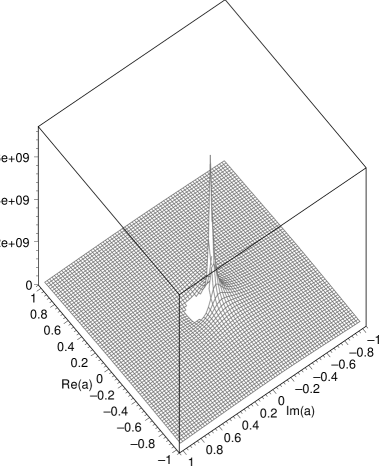
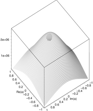
FIG. 1.: Part a: the parameter $\hat{\alpha}^{2}$ as a function of $a$ (real and imaginary part) for the first solution (82); Part b: same parameter for the second solution (83)

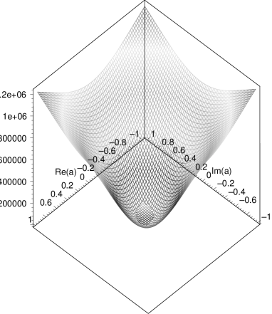
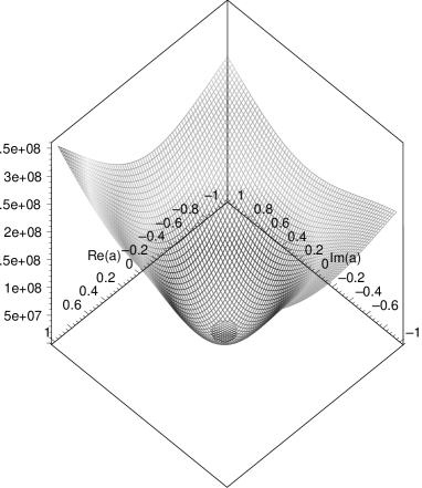
FIG. 2.: Part a: the parameter $\hat{\beta}^{2}$ as a function of $a$ (real and imaginary part) for the first solution (82); Part b: same parameter for the second solution (83)

REFERENCES

• [1] e-mail address: falk@thep.physik.uni-mainz.de
• [2] e-mail address: haeussli@thep.physik.uni-mainz.de
• [3] e-mail address: scheck@thep.physik.uni-mainz.de
• [4] G.C. Branco, L. Lavoura, and F. Mota, Phys. Rev. D 39 (1989) 3443
• [5] K. Harayama and N. Okamura; Phys. Lett. B 387 (1996) 614
• [6] F.D. Murnaghan, The Theory of Group Representations, Dover Publ. New York, 1963; The Unitary and Rotation Groups, Spartan Books, Washington D.C. 1962
• [7] R. Häußling and F. Scheck, Phys. Let.t B 336 (1994) 477
• [8] R. Häußling and F. Scheck, Phys. Rev. D 57 (1998) 6656
• [9] Review by F.J. Gilman, K. Kleinknecht, and B. Renk, in Eur. J. of Physics C15 (2000) 110
• [10] S. Falk, diploma thesis, Johannes Gutenberg-University Mainz, November 2001
• [11] E. Takasugi, The rephasing freedom and the NNI form of quark mass matrices, 1997, hep-ph/9705263;
E. Takasugi, M. Yoshimura; Reconstruction of quark mass matrices in the NNI form from the experimental data, 1997, hep-ph/9709367
Y. Koide, Mod. Phys. Lett. A 12 (1997) 2655
Refer to caption
Refer to caption