Partial Deconfinement in Color Superconductivity

Abstract

We analyze the fate of the unbroken SU(2) color gauge interactions for 2 light flavors color superconductivity at non zero temperature. Using a simple glueball lagrangian model we compute the deconfining/confining critical temperature and show that is smaller than the critical temperature for the onset of the superconductive state itself. The breaking of Lorentz invariance, induced already at zero temperature by the quark chemical potential, is shown to heavily affect the value of the critical temperature and all of the relevant features related to the deconfining transition. Modifying the Polyakov loop model to describe the SU(2) immersed in the diquark medium we argue that the deconfinement transition is second order. Having constructed part of the equation of state for the 2 color superconducting phase at low temperatures our results may be relevant for the physics of compact objects featuring a two flavor color superconductive state.

I Introduction

Quark matter at very high density is expected to behave as a color superconductor REV . Possible physical applications are related to the physics of compact objects REV , supernovae cooling Carter:2000xf and explosions HHS as well as to the Gamma Ray Bursts puzzle OS . Here we concentrate on some features related to color superconductivity with 2 light flavors (2SC). The low-energy effective Lagrangian describing the in medium fermions and the broken sector of the $SU_{c}(3)$ color groups for the 2 flavor color superconductor (2SC) has been constructed in Ref. CDS ; OS2 . The 3 flavor case (CFL) has been developed in CG ; Casalbuoni:1999zi . The effective theories describing the electroweak interactions for the low-energy excitations in the 2SC and CFL case can be found in CDS2001 . The global anomalies matching conditions and constrains are discussed in S . An interesting property of the $2SC$ state is that the three color gauge group breaks spontaneously to a left over $SU(2)$ subgroup and it can play a role for the physics of compact objects OS . In Reference rischke2k it has been shown that the confining scale of the unbroken $SU(2)$ color subgroup is lighter than the superconductive gap $\Delta$. The confined degrees of freedom, glueball-like particles, are expected to be light with respect to $\Delta$, and the effective theory based on the anomalous variation of the dilation current has been constructed in OS2 .

Clearly for the physics of compact objects and more generally for a complete understanding of the QCD phase diagram it is relevant to know at what temperature the $SU(2)$ color gauge group confines/deconfines, the order of the phase transition and the equation of state.

Investigating the deconfinement phase transition is, in general, a complex problem. At zero density importance sampling lattice simulations are able to provide vital information about the nature of the temperature driven phase transition for 2 and 3 colors Yang-Mills theories with and without matter fields (see Karsch:2001jb for a review). Different models Campbell:ak ; Simonov:bc ; Agasian:fn ; Sollfrank:du ; Carter:1998ti ; Schaefer:2001cn ; Drago:2001gd ; Renk:2002md ; Pisarski:2001pe ; DP ; KorthalsAltes:1999cp ; Dumitru:2001xa ; Scavenius:2002ru ; Wirstam:2001ka are used in literature to tackle/study the features of this phase transition from a theoretical stand point. Some models compute non zero temperature corrections for the glueball Lagrangian with or without elementary gluon degrees of freedom (the latter added to describe the deconfined side of the phase transition). Others rely on mean field theories encoding the symmetries of the Polyakov loops Pisarski:2001pe .

Hence we consider a simple, but predictive, model for the deconfinement temperature which makes use of the glueball Lagrangian valid at non zero quark density OS2 . We investigate the one loop thermal effective potential corrections for the dilatonic Lagrangian and observe that as we increase the temperature a new local minimum sets in for a lower value of the gluon condensate with respect to the zero temperature one. The critical temperature is defined as the value for which the two local minima have the same free energy value. Above this critical temperature the model is no longer applicable since new degrees of freedom like the unconfined gluons are expected to appear (see e.g. Carter:1998ti ) and we will briefly comment on their effects. An amusing feature of the model is that the critical temperature can be determined analytically. This is so since the new minimum appears for a zero vacuum expectation value of the gluon condensate and at this point, in the one loop approximation, one can exactly compute the effective thermal potential yielding the following estimate for the critical temperature:

$$T_{c}=\sqrt[4]{\frac{90\,v^{3}}{2e\pi^{2}}}\hat{\Lambda}\ .$$ (1)

Here $e$ is the Euler number, $\hat{\Lambda}$ is the confining scale of the $SU(2)$ gluon-dynamics in 2SC and $v$ is the gluon rischke2k as well as light glueball velocity OS2 . Equation (1) is a good approximation also for the in vacuum theory. Here when Eq. (1) is adjusted to take into account the gluonic degrees of freedom the higher order (in loop) contributions are shown to be less than 10% (see Carter:1998ti ).

We find that the deconfining/confining critical temperature is smaller than the critical temperature $T_{2SC}$ for the superconductive state itself which is estimated to be $T_{2SC}\approx 0.57~{}\Delta$ with $\Delta$ the 2SC gap PR . Actually the breaking of Lorentz invariance, due to the quark chemical potential and encoded in the glueball velocity, further reduces the critical temperature by a factor $v^{3/4}$ relative to the in vacuum case. This is a general feature independent of the model Lagrangian, also observed in Casalbuoni:1999zi . The temperatures in play are much less than the value of the quark chemical potential. The situation is more involved if also rotational invariance breaks spontaneously due, for example, to the appearance of a spin one condensate Sannino:2001fd . We study the glueball mass as function of temperature, chemical potential and $\Delta$. In the confined phase the mass is, at a very good approximation, constant with respect to the temperature.

By computing the glueball thermal effective potential we provide part of the equation of state for the 2SC phase at low temperatures. In particular we can compute the pressure, the energy density and the entropy of the system below the critical deconfining temperature.

It is important to stress that in this paper we are considering an ideal 2SC state where the up and down quarks are massless and the strange quark is infinitely massive. When computing properties related to the physics of compact stars it is very important to introduce in the model the effects of the quark masses as well as the ones induced by a not too heavy strange quark. These effects may affect the $SU(2)$ gluon properties and can be investigated using for example the effective theories near the fermi surface REV . It would also be very interesting to see how the non perturbative $SU(2)$ dynamics might affect the recent results in Alford:2002kj . However even within the present restrictive framework our estimate for the $SU(2)$ confining temperature may be a useful guide for astrophysical models of compact stars like the one in Ref. OS featuring a 2SC state.

Since the gluon-condensate is not a true order parameter for the deconfining transition the glueball Lagrangian cannot be used to infer the order of the transition itself. To settle this issue we modify the Polyakov’s loop inspired model Pisarski:2001pe to fit the present case and finally predict a second order phase transition. Finally we suggest how ordinary lattice importance sampling techniques can be used to check our results and constitute, at the same time, the first simulations testing the high quark chemical potential but small temperature region of the QCD phase diagram.

The glueball Lagrangian, if extended to describe the transition point, predicts a first order transition which seems to disagree with the prediction based on the order parameter (Polyakov’s loop). Actually the disagreement is an apparent one. Indeed only the order parameter is obliged to know about the order of the phase transition. Any other gauge invariant quantity does not need to display the same behavior while still bearing information about the phase transition itself (see for example Pisarski:2001pe page 3 equations (9) and (10) and subsequent discussion (first reference)). In practice the critical temperature predicted represents also the limit of applicability of our simple model. At the critical point the Ginzburg-Landau theory for the order parameter is the proper way to describe the transition itself and can be used to infer the order of the phase transition. Unfortunately though the Ginzburg-Landau theory cannot predict the critical temperature. The previous discussion does not imply that the glueball and the order parameter (the Polyakov loop) at the transition are not related Sannino:2002wb .

It is important to stress that in general we have a tower of scalar, pseudoscalar and other excited glueball states in the confined regime together with the other physical states involving quarks of the 2SC state. We have made the standard assumption that the low energy $SU(2)$ dynamics is dominated by the associated lightest mode in the theory: the scalar glueball. This state does not couple to the light ungapped up and down quarks in the direction 3 of color (for a review of the complete low energy effective theory of the 2SC state see the 7th reference in REV ). Besides, according to Litim:2001je , the quark temperature effects are exponentially suppressed ($\sim\exp({-\Delta/T})$) so for $T<T_{c}$ and $\hat{\Lambda}<\Delta$, for an initial investigation, we can neglect these corrections. For temperatures in the range $T_{c}<T<T_{2SC}$ the gapped quark dynamics is no longer negligible and some of their effects have been computed using transport theory in Litim:2001je . Our model must be considered only as a first step toward a more complete theory of the 2SC state where the $SU(2)$ non perturbative dynamics is included.

In Section II we provide the light glueball Lagrangian and construct the one loop thermal effective action. Here we suggest a way to relate the results obtained by employing different parameterizations for the glueball field. In Section III we study the relevant features connected with the deconfining transition. We provide an economical criterion to estimate the critical temperature similar to the one extensively used in literature for the in vacuum Yang-Mills theories Carter:1998ti . Finally using the Polyakov loop model adapted to the present case we show the phase transition to be likely second order. We conclude in Section IV.

II Glueball Effective Lagrangian at finite Temperature

The light glueball action for the in–medium Yang-Mills theory is OS2 :

$$S_{Glueball}=\int d^{4}x \left\{\frac{c}{2}\,H^{-\frac{3}{2}}\left[\partial^{0}H\partial^{0}H-v^{2}\partial^{i}H\partial^{i}H\right]-\frac{1}{2}H\log\left[\frac{H}{\hat{\Lambda}^{4}}\right]\right\}\ .$$ (2)

$H$ is the composite field describing, upon quantization, the scalar glueball OS2 ; schechter ; SS ; SSSusy ; MS ; SST ; GJJK ; CE in medium and possesses mass-scale dimensions four. Here $c$ is a positive constant which fixes the tree glueball mass. Our results do not depend on the specific value assumed by this constant. It is also important to stress that the glueballs move with the same velocity as the underlying gluons in the 2SC color superconductor OS2 . The velocity depends on the gluon dielectric constant ($\epsilon$) and magnetic permeability ($\lambda$) via $v=1/\sqrt{\epsilon\lambda}$. The dielectric constant $\epsilon$ is different from unity (in fact $\epsilon\gg 1$ in the 2SC case rischke2k ) leading to an effectively reduced gauge coupling constant. Studying the polarization tensor at asymptotically high quark densities for the $SU(2)$ gluons in rischke2k was found:

$$\epsilon=1+\frac{g_{s}^{2}\mu^{2}}{18\pi^{2}\Delta^{2}}\ ,\qquad\lambda=1\ ,$$ (3)

with $g_{s}$ the underlying $SU(3)$ coupling constant and $\mu$ the quark chemical potential. This result has also been derived via effective theories valid close to the Fermi surface Casalbuoni2001 . In the effective Lagrangian $\hat{\Lambda}$ is a physical constant related to the confining scale of the in– medium 2 color Yang-Mills theory. Following rischke2k we have the one loop relation:

$$\hat{\Lambda}=\Delta\exp\left[-\frac{8\pi^{2}}{bg_{s}^{2}(\mu)}{\sqrt{\frac{\epsilon(\mu/\Delta)}{\lambda(\mu/\Delta)}}}\right]\simeq\Delta\exp\left[-\frac{2\sqrt{2}\pi}{11}\frac{\mu}{g_{s}(\mu)\Delta}\right]\ ,$$ (4)

with $b=22/3$ (at one loop) for $SU(2)$ and in the last step we considered the asymptotic solution of Ref. rischke2k , for convenience reported in Eq. (3). By using $\Lambda_{QCD}\simeq 300$ MeV, $\mu\simeq 500$ MeV and a gap value of about $30$ MeV one gets $\hat{\Lambda}\simeq 1$ MeV. It is hence reasonable to expect that the glueballs are light (with respect to the gap) with a mass typically somewhat larger or of the order of the confining scale. They are stable with respect to the strong interactions unlike ordinary glueballs while still decaying into two photons OS2 . The potential in Eq. (2) can be considered a zeroth order model schechter ; MS ; SST for a Yang-Mills theory in medium OS2 in which the glueballs are the associated hadronic particles. The minimum of the potential $V$ (see OS2 for details) is taken for

$$\langle H\rangle=\frac{\hat{\Lambda}^{4}}{e}\ ,\quad{\rm at~{}which~{}point}\quad\langle{V}\rangle=-\frac{\hat{\Lambda}^{4}}{2\,e}\ .$$ (5)

For the zero density case a number of phenomenological questions have been discussed using this type of toy model Lagrangian Eq. (2) SST .

In order to extract dynamical information we define a canonically normalized (with canonical mass dimension one) glueball field $h$ via:

$$H=f(h)=f_{(0)}^{4}+f_{(1)}h+f_{(2)}\frac{h^{2}}{2!}+\cdots+f_{(n)}\frac{h^{n}}{n!}+\cdots\ ,$$ (6)

where we require $f(h)$ to be a well behaved function of the glueball field $h$ with non vanishing $f_{(0)}$ and $f_{(1)}$. The normalization condition of the kinetic term, at the tree level, yields the constraint:

$$c^{\frac{1}{2}}\,f_{(1)}=f_{(0)}^{3}\ .$$ (7)

It is reasonable to expect that any interpolating function $f(h)$ should lead to the same physical results. This is indeed the case at the tree level since all of the possible choices to define a canonically normalized field are equivalent.

However when considering thermal/quantum corrections is hard to demonstrate that different choices lead to the same physical results. We remind the reader of the time-honored sigma model example where the linear version is a renormalizable theory while the non linear sigma model is not a renormalizable theory in the usual sense.

In order to keep our results as independent as possible from the specific function $f(h)$ here we define thermal averages directly in terms of $H$. More specifically following Dolan and Jackiw Dolan:qd we formally introduce the temperature effective action $\Gamma(\overline{H})$ -the generating functional for single-particle irreducible Green’s functions via:

$$W[J] = -i\log\left[\frac{{\rm Tr}e^{-\frac{\cal H}{T}}\exp\left[i\int d^{4}x\,H(x)J(x)\right]}{{\rm Tr}e^{-\frac{\cal H}{T}}}\right]\ ,$$ (8)

$$\overline{H}(x) = \frac{\delta W[J]}{\delta J(x)}\ ,$$ (9)

$$\Gamma[\overline{H}] = W[J]-\int d^{4}x\,{\overline{H}}(x)J(x)\ .$$ (10)

${\cal H}$ is the Hamiltonian and $J(x)$ the external source for the gluon condensate. In the last equation $J(x)$ is eliminated in favor of $\overline{H}(x)$ by the definition in (9). We also have that ${\delta\Gamma[\overline{H}]}/{\delta\overline{H}(x)=-J(x)}$ and $\overline{H}(x)$, evaluated at $J=0$, is the thermodynamic average of the gluon condensate field $H(x)$. The present definition of the effective action is independent of the choice of the interpolating field function. For the present purposes it is sufficient to study $\Gamma[\overline{H}]$ for constant ${\overline{H}}(x)$ and consider the effective potential:

$$V[\overline{H}]=-\frac{\Gamma[\overline{H}]}{\rm{space-time~{}volume}}\ .$$ (11)

In practice the $J$ dependent tree generating functional for the trace anomaly is (with $V\left[J\right]=-W\left[J\right]/(\rm{space-time~{}volume})$ for constant fields)

$$V_{Tree}[J]=\frac{1}{2}H\log\left[\frac{H}{\hat{\Lambda}^{4}}\right]-J\,H\ .$$ (12)

and the one loop thermal effective potential as function of $J$ is:

$$V[J] = {2}f_{(0)}^{4}\log\left[\frac{f_{(0)}}{\hat{\Lambda}}\right]-J\,f_{(0)}^{4}+\frac{T}{v^{3}\,2\pi^{2}}\int_{0}^{\infty}dk\,k^{2}\log\left[1-\exp\left({-\frac{\epsilon_{J}}{T}}\right)\right]\ ,$$ (13)

where $\displaystyle{\epsilon_{J}=\sqrt{k^{2}+M^{2}_{J}\left(f_{(0)},f_{(2)}\right)}}$, and $M^{2}_{J}$ is defined via the curvature of the potential as

$$M^{2}_{J}=\left.\frac{\partial^{2}V}{\partial h^{2}}\right|_{h=0}=\frac{f_{(0)}^{2}}{2c}+f_{(2)}\left[2\log\frac{\sqrt[4]{e}\,f_{0}}{\hat{\Lambda}}-J\right]\ .$$ (14)

With the help of

$$\overline{H}\equiv\overline{h}^{4}=-\frac{\delta V\left[J\right]}{\delta J}=f_{(0)}^{4}+\frac{f_{(2)}}{v^{3}4\pi^{2}}\,\int_{0}^{\infty}\frac{dk\,k^{2}}{\left[\exp\left(\displaystyle{\frac{\epsilon_{J}}{T}}\right)-1\right]\,\epsilon_{J}}\ ,$$ (15)

we deduce the effective potential

$$V[\overline{h}]=\left[1-J\,\frac{\partial}{\partial J}\right]V[J]\ ,$$ (16)

where the functional derivative with respect to $J$ is replaced with a partial derivative since we are now dealing with constant fields. We need now to solve for $J[\overline{H}]$ as function of $\overline{H}$ and then extremize the action. We identify $\bar{H}$ with $\bar{h}^{4}$ only after $J$ has been eliminated. For a general choice the function $f(h)$ one cannot find an analytical expression for $J[\overline{H}]$. However we immediately notice that for $f_{(2)}=0$ (at the one-loop level) there is no dependence on $J$ and we have $\overline{h}=f_{(0)}$ as well as a positive definite curvature $M^{2}={f_{(0)}}^{2}/{2c}$. To be more specific our glueball field function is now $f(h)=f_{(0)}^{4}+f_{(1)}\,h$ where we truncate our function to the quadratic term since higher terms do not affect the one loop result. Actually any function $f(h)$ with just vanishing $f_{(2)}$ leads to the same source independent effective thermal potential:

$$V\left[\bar{h}\right]={\hat{\Lambda}^{4}\over 2e}+2\bar{h}^{4}\log\left[\frac{\bar{h}}{\hat{\Lambda}}\right]+\frac{T^{4}}{v^{3}\,2\pi^{2}}\int_{0}^{\infty}dx\,x^{2}\log\left[1-\exp\left(-\sqrt{x^{2}+\frac{\bar{h}^{2}}{2cT^{2}}}\right)\right]\ ,$$ (17)

where for convenience we subtracted the constant value of the potential evaluated on the vacuum at zero temperature. This expression is well defined for any value of $\bar{h}$. $V\left[\bar{h}\right]$ is shown in Fig. 1 for different values of the temperature and a given value of $c$ which fixes the zero temperature tree-level glueball mass (i.e. $M^{2}=\hat{\Lambda}^{2}/2\sqrt{e}c$). The plot is provided only for illustration and the general feature of the potential does not change for different choices of the chemical potential and reasonable values of the gap parameter. Note that our results for the critical temperature (presented in the next section) are evaluated at different values of the quark chemical potential and the gap $\Delta$. As we increase the temperature we observe a new minimum setting in for $\bar{h}$ at zero. We also note that the position of the old minimum is not much affected by temperature corrections over a large range of temperatures (see Fig. 1). Close to the new minimum at zero is possible to perform the high temperature expansion leading to:

$$\lim_{\bar{h}\rightarrow 0}V\left[\bar{h}\right]={\hat{\Lambda}^{4}\over 2e}-\frac{2\pi^{2}}{90}\frac{T^{4}}{v^{3}}+\frac{\bar{h}^{2}}{2c}\frac{T^{2}}{24v^{3}}+{\cal O}\left(\bar{h}^{4}\right)\ .$$ (18)

Before describing in some detail the features of the phase transition we now briefly comment on another possible choice of the glueball field widely used in literature. This is the exponential representation:

$$H=f_{(0)}^{4}\exp\left[\frac{h}{f_{(0)}\sqrt{c}}\right]\ .$$ (19)

This function recovers the previous one for small field fluctuations. However since $f_{(2)}=f_{(0)}^{2}/c$ is not vanishing we cannot deduce an analytical expression of $J$ as function of $\bar{h}$. Note that if we would naively set $J$ to zero from the beginning the second derivative of the potential defined in Eq. (14) is not definite positive for all values of $\bar{h}$ and the integral in Eq. (17) is ill defined. Often in the literature the thermal corrections are computed without including the source $J$. We have shown that, at the one loop level, the linearly realized representation is not affected by the introduction of the source term while the non linear realization used for example in Drago:2001gd are very much affected and should be handled with care. We expect the partial derivative term $J\partial V[J]/\partial J$ in Eq. (16) to help compensating for the possible different choices of $f(h)$. In the rest of this work we shall use the linear realizations.

Clearly after having defined the extremum of the effective potential it is a simple matter to derive all of the relevant thermodynamical quantities. For the reader’s convenience we summarize the standard relations between the thermodynamical quantities and the free energy (per unit volume) $F=V$ (V is evaluated on the minimum) with the pressure $P=-F$ while the entropy per unit volume is $S=-\partial F/\partial T$.

Figure 1: Potential function $V\left[\bar{h}\right]/\hat{\Lambda}^{4}$ for $\mu=500$ MeV and $\Delta=30$ MeV as function of the condensate $\bar{h}/\hat{\Lambda}$ for different values of the temperature. The solid line corresponds to $T=0$; the dotted line to $T=0.85~{}T_{c}$; the short-dashed to $T=T_{c}$; the long dashed to $T=1.1~{}T_{c}$. Finally the dot-dashed line corresponds to the high temperature expansion near $\bar{h}=0$ for $T=1.1~{}T_{c}$. We have chosen for definitiveness $c=1/(50\sqrt{e})$, corresponding to a zero temperature glueball mass of $5\hat{\Lambda}$.

III Relevant features of the deconfining transition

Studying the one loop thermal effective potential in Eq. (16) one observes that when increasing the temperature a new local minimum sets in at $\bar{h}=0$ and, for a certain range of temperatures, the potential has two local minima. The temperature for which the two minima have the same free energy is:

$$T_{c}=\sqrt[4]{\frac{90\,v^{3}}{2e\pi^{2}}}\hat{\Lambda}\ .$$ (20)

This value is obtained by comparing the jump of the potential due to the temperature corrections (actually at zero $\bar{h}$) with the respect to the zero temperature minimum, and it does not depend on the specific value assumed by the constant $c$ in the effective Lagrangian. The latter can be fixed once the glueball mass is known.

Assuming that the drop in the gluon condensate together with the drastic change in the glueball mass are related to the deconfinement phase transition as supported by lattice simulations Bacilieri we interpret Eq. (1) as an estimate for the critical temperature. In figure 2 we plot the critical temperature as function of the superconductive gap for different values of the quark chemical potential. In models where the contribution of the elementary gluons is added one finds a smaller temperature (see for example Carter:1998ti ). The reduction is due to the extra contribution of the light gluons appearing at $T_{c}$. This effect can be estimated assuming that the main contribution of the gluons at $T_{c}$ is the free energy for unconfined gluons propagating with velocity $v$. By simply adding to the effective thermal potential the term $-2\pi^{2}\left[2(N^{2}-1)\right]T^{4}\Theta(T-T_{c})/(90v^{3})$ for a general number of colors $N$ the temperature for which the two minima have the same free energy value is lowered to

$${T}_{c}\rightarrow\frac{T_{c}}{\sqrt[4]{2\left(N^{2}-1\right)+1}}\ .$$ (21)

The reduction is perhaps too drastic since, in many investigations at zero density, it has been argued that a better fit to the Lattice data even at temperatures as high as 3 times the critical temperature requires an effective number of gluon degrees of freedom lower than the one predicted by a free gas approximation. It is then quite likely that the true critical temperature lies in between the one presented in Eq. (1) computed without gluons and the one estimated Eq. (21).

When reducing the temperature from the quark gluon plasma phase we see that color superconductivity first sets in along the temperature axis with the $SU(2)$ of color still unconfined and finally the $SU(2)$ confines at a lower value of the temperature (see Fig. 2). Higher order corrections to our critical temperature are shown to be smaller than 10% (see Carter:1998ti ).

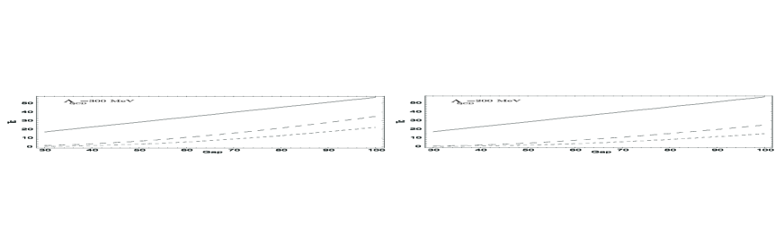
Figure 2: Plots of the $SU(2)$ critical temperature for 2 values of the quark chemical potential ($\mu=400$ MeV long–dashed line; $\mu=500$ MeV short–dashed line) as function of the superconductive gap $\Delta$. The solid line corresponds to the critical temperature for the superconductive state $0.57\Delta$. The left panel corresponds to $\Lambda_{QCD}=300$ MeV while the right one corresponds to $\Lambda_{QCD}=200$ MeV

We also see confronting the left and right panel of Fig. 2 that the critical temperature decreases if $\Lambda_{QCD}$ decreases.

Our model applies directly only to the ideal 2SC state and for physical applications we need to consider in some detail the corrections induced for example by the quark masses. Nevertheless it might be instructive to show how the explicit dependence of the $SU(2)$ confining temperature on $\mu$ and $\Delta$ may be helpful to astrophysical applications. Indeed in a model for Gamma Ray Bursts (GRBs) OS it was suggested that some compact stars might feature a hot 2SC surface layer. The GRBs model used the glueballs as an active degree of freedom. So we need to know when, along the temperature axis, the 2SC layer enters the $SU(2)$ confining regime. Within our model calculations we indicate in the $T-\mu$ phase diagram where the glueballs degrees of freedom start playing a role. For example if $\mu=400-500$ MeV from Fig. 2 we deduce that the $SU(2)$ confines at $T_{c}\approx 10$ MeV provided $\Delta\geq 60-70$ MeV. Our work might also be useful when investigating the cooling process in compact stars.

The derived free energy for the $SU(2)$ glue for very low temperatures represents an initial step when computing part of the complete equation of state which is needed when considering the thermodynamics of compact object featuring a 2SC state. In our model we have assumed the glueball velocity not to depend on the temperature. This is reasonable since the temperature corrections for $v$ are exponentially suppressed, more specifically the suppression factor is $e^{-\Delta/T}$ Rischke:2001py ; Litim:2001je . Since we find the critical temperature to lie well below the critical temperature for color superconductivity ($T_{2SC}\approx 0.57\Delta$) our results provide a consistent picture. It is important to stress that for temperatures $T_{c}<T<T_{2SC}$ the gapped quark contributions are no longer negligible. In Ref. Litim:2001je using the transport theory some relevant temperature effects have been analyzed.

It is useful to study the dependence of the glueball mass on the temperature. Defining the square of the mass as the potential curvature evaluated at the (global) minimum we observe (see Fig. 1) that for $T<T_{c}$ the curvature is practically constant and the mass square value is well approximated by $M^{2}(T<T_{c})=\hat{\Lambda}^{2}/{2\sqrt{e}c}$ .

Although the glueball treatment alone cannot be used above the deconfining phase transition it is nevertheless interesting to consider such a temperature region. For $T\geq T_{c}$ the new global minimum is at zero and we can use Eq. (18) to deduce

$$\frac{M^{2}(T\geq T_{c})}{M^{2}(T=0)}=\frac{\sqrt{5}}{4\pi\sqrt{v^{3}}}\left[\frac{T}{T_{c}}\right]^{2}\ .$$ (22)

Due to the velocity factor in Eq. (22) there is a relative enhancement with to the respect to the in vacuum (but hot) Yang-Mills theory. For illustration we plot our results in Fig. 3 for the in vacuum (i.e. $v=1$ and $\mu=0$) and the in medium theory for $\mu=500$ while considering different values of $\Delta$.

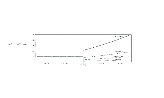
Figure 3: Illustrative plot of the glueball mass as function of the temperature , $M^{2}(T)/M^{2}(T=0)$ for different values of $\Delta$ and fixed chemical potential $\mu=500$ MeV. The curve labelled by $\mu=0$ corresponds to the in vacuum (but hot) case. It is straightforward to consider another value of $\mu$ and the qualitative picture remains unchanged.

Since the glueball mass increases in the deconfined phase the new light degrees of freedom (namely the elementary gluons themselves) now dominate the free energy. Interestingly we find that due to a large dielectric constant of the 2SC medium the associated light glueballs mass square in the deconfined region gains a factor $1/\sqrt{v^{3}}$ relative to the in vacuum case. Hence for all of the relevant thermodynamical properties/quantities of the 2SC above the deconfining $SU(2)$ phase transition the glueballs are not expected to play an important role. Since we plot the ratio of masses the result does not depend on the positive constant $c$. From the figure is also clear that there is a strong dependence on the specific value of $\Delta$.

We now comment briefly on the fate of the old minimum as the temperature is increased above the critical temperature and in absence of elementary gluons. The value of the glueball condensate corresponding to the old minimum just above the critical temperature start reducing while the minimum disappears for a temperature of the order of $\approx 2T_{c}$. This behavior is summarized in Fig. 4 and it is a classical example of first order phase transition if we were to consider the glueball Lagrangian as the correct description at and above the transition point.

Figure 4: Zoom of the Potential of Eq. (17) close to the old minimum for $\mu=500$ MeV, $\Delta=30$ MeV as function of the condensate $\bar{h}/\hat{\Lambda}$ for different values of the temperature above $T_{c}$. The solid line corresponds to $T=T_{c}$, the dotted line to $T=1.8~{}T_{c}$, the short-dashed to $T=1.9~{}T_{c}$ and the long dashed to $T=2~{}T_{c}$. We have, as in Fig. 1, chosen $c=1/(50\sqrt{e})$.

When restricting to the in vacuum theory our results are in reasonable agreement with the results and expectations of various investigations (see for example Carter:1998ti and references therein) using similar models.

The glueball Lagrangian based model cannot be used to establish the order of the phase transition since the gluon condensate is not an order parameter for a Yang-Mills theory although it does encode information on the underlying conformal anomaly. The break down point signals the presence of new lighter degrees of freedom which needed to be taken into account. In the absence of quarks a reasonable order parameter for the $SU(N)$ Yang-Mills theory is the Polyakov loop Svetitsky:1982gs :

$${\ell}\left(x\right)=\frac{1}{N}{\rm Tr}({\bf L})\equiv\frac{1}{N}{\rm Tr}\left[{\cal P}\exp\left[i\,g\int_{0}^{1/T}A_{0}(x,\tau)d\tau\right]\right]\ ,$$ (23)

where ${\cal P}$ denotes path ordering, $g$ is the $SU(N)$ coupling constant and $x$ is the coordinate for the three spatial dimensions while $\tau$ is euclidean time. The $\ell$ field is real for $N=2$ while otherwise complex. This object is charged with respect to the center $Z_{N}$ of the $SU(N)$ gauge group Svetitsky:1982gs under which it transforms as $\ell\rightarrow z\ell$ with $z\in Z_{N}$. A relevant feature of the Polyakov loop is that its expectation vanishes in the low temperature regime and is non zero in the high temperature phase.

This behavior has recently lead Pisarski Pisarski:2001pe to model the Yang-Mills (non supersymmetric) phase transition as a mean field theory of Polyakov loops. One can simply show that for $SU(2)$ one expects a second order phase transition (as function of the temperature) and a weak first order for $SU(3)$.

We can use Pisarski’s model to predict the order of the transition in the present case. Assuming that a local $SU(2)$ Yang-Mills action at low energies does exists we construct the simplest Polykov loop using the rescaled space time coordinates and fields rischke2k ; OS2 :

$${\hat{\ell}}\left(x\right)=\frac{1}{2}{\rm Tr}\left[{\cal P}\exp\left[i\,\hat{g}\int_{0}^{1/\hat{T}}\hat{A}_{0}({x},\hat{\tau})d\hat{\tau}\right]\right]\ ,$$ (24)

with $\hat{A_{0}}=\hat{A}_{0}^{a}\tau^{a}/2$ and $\tau^{a}$ the $SU(2)$ Pauli matrices, and the connection with the underlying fields is rischke2k ; OS2 $\hat{A_{0}^{a}}=\lambda^{\frac{1}{4}}\epsilon^{\frac{3}{4}}A_{0}^{a}$ while $\hat{g}=g_{s}(\lambda/\epsilon)^{\frac{1}{4}}$. The rescaled euclidean time $\hat{\tau}=\tau/\sqrt{\lambda\epsilon}$ leads to $\hat{T}=T/v$ while $\lambda$ is a possible magnetic permeability which turns to be equal to one in our case. At this point the effective mean field type of model a lá Pisarski for $\hat{\ell}$ is similar to the one for the in vacuum $SU(2)$ Yang-Mills theory. So if we make the strong but plausible assumption (as shown above) that all the way up and above the deconfinement $SU(2)$ color phase transition the effects of the quark superconductive matter can be taken into account just via a non zero dielectric constant we expect a second order phase transition for the $SU(2)$ of color in 2SC. It is relevant to mention that the order of the transition might change if we include new contributions arising for example by considering the quark masses. The deconfining temperature is expected to be the one close to our prediction obtained from the glueball model Lagrangian. Even if a non zero magnetic permeability exists the present argument would not be modified.

$SU(2)$ Yang-Mills with non zero dielectric and magnetic permeability can be simulated, using standard sampling methods, on the lattice. For a large body of work on $SU(2)$–Yang–Mills theory we refer to Damgaard . These results would test at the same time the validity of the glueball model for the prediction of the critical temperature and the order of the phase transition according to the Polyakov loop model in a framework slightly modified with respect to the in vacuum case. Besides the latter would also constitute the first lattice simulations testing the high quark chemical potential but small temperature region of the QCD phase diagram.

The disagreement between the first order phase transition predicted by the glueball Lagrangian and the previous argument based on the symmetries obeyed by the order parameter is an apparent one. In fact any gauge invariant quantity which is not an order parameter does not need to behave as the order parameter itself at the transition Pisarski:2001pe as discussed at length in the introduction (see also Sannino:2002wb ).

IV Conclusions

We studied the temperature effects on the unbroken $SU(2)$ color gauge interactions for the 2 flavor case at high matter density. Using a simple model based on a light glueball Lagrangian we estimated the $SU(2)$ deconfinement critical temperature for given chemical potential and superconductive gap value. We have shown that the deconfining/confining critical temperature is smaller than the critical temperature for the superconductive state itself. The breaking of Lorentz invariance (already at zero temperature), encoded in the glueball velocity, further reduces the critical temperature by a factor $v^{3/4}$ relative to the in vacuum case. By computing the glueball thermal effective potential we have the equation of state for part of the ideal 2SC phase (i.e. zero up and down quark masses and infinitely massive strange quark). In particular we can compute the pressure, the energy density and the entropy of the system.

Another relevant point is that we have developed a general framework according to which any parameterization of the glueball field can be used to construct the full thermal effective action arising from the lagrangian constructed using the anomalous variation of dilation current.

Using the Polyakov loop model, adapted to the present case we also predict the associated phase transition to be second order.

In order to apply our model to the physics of compact objects we should extend it in order to take into accounts the effects of the the up and down quark masses as well as the effects of a not too massive strange quark.

Notes added in proof

About two months after we submitted this paper the paper Alford:2002kj appeared where it is claimed that the 2SC state might not be present on compact stars. This is a very dynamical issue which deserves further studies. The present paper deals with the properties of part of the ideal 2SC state and as such our results are not affected by this claim. However possible astrophysical applications may be affected. Finally also Ref. Sannino:2002wb which clarifies the relation between the order parameter and the gluon condensate further strengthening our approach appeared after this paper was submitted.

- (1) See K. Rajagopal and F. Wilczek, hep-ph/0011333; M.G. Alford, Ann. Rev. Nucl. Part. Sci. 51, 131 (2001) [arXiv:hep-ph/0102047] for an overview on the subject; S.D.H. Hsu, hep-ph/0003140 for the renormalization group approach review; D.K. Hong, Acta Phys. Polon. B32:1253, 2001, hep-ph/0101025 for the effective theories close to the fermi surface; R. Casalbuoni, AIP Conf. Proc. 602, 358 (2001) [arXiv:hep-th/0108195]. for the effective Lagrangians approach. G. Nardulli, hep-ph/0202037 for the effective theory approach to CSC and the LOFF phase and possible applications of the LOFF phase to the physics of compact stars; F. Sannino, hep-ph/0112029 for the 2SC effective Lagrangians, topological terms and the electroweak sector.
- (2) G. W. Carter and S. Reddy, Phys. Rev. D 62, 103002 (2000), hep-ph/0005228.
- (3) D. K. Hong, S. D. Hsu and F. Sannino, Phys. Lett. B 516, 362 (2001), hep-ph/0107017.
- (4) R. Ouyed and F. Sannino, astro-ph/0103022.
- (5) R. Casalbuoni, Z. Duan and F. Sannino, Phys. Rev. D 62 (2000) 094004, hep-ph/0004207.
- (6) R. Ouyed and F. Sannino, Phys. Lett. B 511 (2001) 66 hep-ph/0103168.
- (7) R. Casalbuoni and R. Gatto, Phys. Lett. B464, 11 (1999).
- (8) R. Casalbuoni and R. Gatto, Phys. Lett. B 469, 213 (1999), hep-ph/9909419.
- (9) R. Casalbuoni, Z. Duan and F. Sannino, Phys. Rev. D 63, 114026 (2001), hep-ph/0011394
- (10) F. Sannino, Phys. Lett. B480, 280, (2000). S. D. Hsu, F. Sannino and M. Schwetz, Mod. Phys. Lett. A 16, 1871 (2001), hep-ph/0006059.
- (11) D. H. Rischke, D. T. Son and M. A. Stephanov, Phys. Rev. Lett. 87, 062001 (2001), hep-ph/0011379.
- (12) F. Karsch, AIP Conf. Proc. 602, 323 (2001) [arXiv:hep-lat/0109017].
- (13) B. A. Campbell, J. R. Ellis and K. A. Olive, Nucl. Phys. B 345, 57 (1990).
- (14) Yu. A. Simonov, JETP Lett. 55, 627 (1992) [Pisma Zh. Eksp. Teor. Fiz. 55, 605 (1992)].
- (15) N. O. Agasian, JETP Lett. 57, 208 (1993) [Pisma Zh. Eksp. Teor. Fiz. 57, 200 (1993)].
- (16) J. Sollfrank and U. W. Heinz, Z. Phys. C 65, 111 (1995), nucl-th/9406014.
- (17) G. W. Carter, O. Scavenius, I. N. Mishustin and P. J. Ellis, Phys. Rev. C 61, 045206 (2000), nucl-th/9812014; G. W. Carter and P. J. Ellis, Nucl. Phys. A 628, 325 (1998), nucl-th/9707051.
- (18) B. J. Schaefer, O. Bohr and J. Wambach, Phys. Rev. D 65, 105008 (2002) [arXiv:hep-th/0112087].
- (19) A. Drago and M. Gibilisco, hep-ph/0112282.
- (20) T. Renk, R. A. Schneider and W. Weise, hep-ph/0201048.
- (21) R. D. Pisarski, hep-ph/0112037; R.D. Pisarski, Phys. Rev. D62, 111501 (2000).
- (22) A. Dumitru and R. D. Pisarski, Phys. Lett. B504, 282 (2001); O. Scavenius, A. Dumitru and A. D. Jackson, Phys. Rev. Lett. 87, 182302 (2001) [arXiv:hep-ph/0103219]; P.N. Meisinger, T.R. Miller, and M.C. Ogilvie, Phys. Rev. D 65, 034009 (2002) [arXiv:hep-ph/0108009]; P.N. Meisinger and M.C. Ogilvie, Phys. Rev. D 65, 056013 (2002) [arXiv:hep-ph/0108026]
- (23) C. P. Korthals Altes, R. D. Pisarski and A. Sinkovics, Phys. Rev. D 61, 056007 (2000), hep-ph/9904305.
- (24) A. Dumitru and R. D. Pisarski, Phys. Lett. B 525, 95 (2002), hep-ph/0106176.
- (25) O. Scavenius, A. Dumitru and J. T. Lenaghan, hep-ph/0201079.
- (26) J. Wirstam, Phys. Rev. D 65, 014020 (2002), hep-ph/0106141.
- (27) R.D. Pisarski and D.H. Rischke, Phys. Rev. D61, 051501 (2000); Phys. Rev. D61, 074017 (2000).
- (28) F. Sannino and W. Schäfer, Phys. Lett. B 527, 142 (2002) hep-ph/0111098; J. T. Lenaghan, F. Sannino and K. Splittorff, Phys. Rev. D 65, 054002 (2002), hep-ph/0107099.
- (29) M. Alford and K. Rajagopal, arXiv:hep-ph/0204001.
- (30) F. Sannino, arXiv:hep-ph/0204174.
- (31) D. F. Litim and C. Manuel, Phys. Rev. Lett. 87, 052002 (2001), hep-ph/0103092.
- (32) R. Casalbuoni, R. Gatto and G. Nardulli, Phys. Lett. B 498 (2001) 179, hep-ph/0010321; R. Casalbuoni, R. Gatto, M. Mannarelli and G. Nardulli, Phys. Lett. B 524, 144 (2002) [arXiv:hep-ph/0107024].
- (33) J. Schechter, Phys. Rev. D21, 3393 (1980). For a review on the effective Lagrangians for QCD see hep-ph/0112205.
- (34) F. Sannino and J. Schechter, Phys. Rev. D60, 056004, (1999).
- (35) F. Sannino and J. Schechter, Phys. Rev. D57, 170 (1998). S. D. Hsu, F. Sannino and J. Schechter, Phys. Lett. B 427, 300 (1998), hep-th/9801097.
- (36) A.A. Migdal and M.A. Shifman, Phys. Lett. 114B, 445 (1982). J.M. Cornwall and A. Soni, Phys. Rev. D29, 1424 (1984); 32, 764 (1985).
- (37) A. Salomone, J. Schechter and T. Tudron, Phys. Rev. D23, 1143 (1981). J. Ellis and J. Lanik, Phys. Lett. 150B, 289 (1985). H. Gomm and J. Schechter, Phys. Lett. 158B, 449 (1985).
- (38) T. De Grand, R.L. Jaffe, K. Johnson and J. Kiskis, Phys. Rev. D12, 2066 (1975). M. Shifman, A. Vainshtein and V. Zakharov, Nucl. Phys. B147, 385 (1979); B147, 448 (1979).
- (39) M.S. Chanowitz and J. Ellis, Phys. Rev. D7, 2490 (1973).
- (40) L. Dolan and R. Jackiw, Phys. Rev. D 9, 3320 (1974).
- (41) P. Bacilieri et al. Phys. Lett. B220, 607, 1989.
- (42) D. H. Rischke, Phys. Rev. D 64, 094003 (2001), nucl-th/0103050.
- (43) B. Svetitsky and L. G. Yaffe, Nucl. Phys. B 210, 423 (1982). L. G. Yaffe and B. Svetitsky, Phys. Rev. D 26, 963 (1982). B. Svetitsky, Phys. Rept. 132, 1 (1986).
- (44) P.H. Damgaard, Phys. Lett. B194 (1987) 107; J. Kiskis, Phys. Rev. D41 (1990) 3204; J. Fingberg, D.E. Miller, K. Redlich, J. Seixas, and M. Weber, Phys. Lett. B248 (1990) 347; J. Christensen and P.H. Damgaard, Nucl. Phys. B348 (1991) 226; P.H. Damgaard and M. Hasenbush, Phys. Lett. B331 (1994) 400: J. Kiskis and P. Vranas, Phys. Rev. D49 (1994) 528. For a more recent review and a rather complete list of references, see S. Hands, Nucl. Phys. Proc. Suppl. 106, 142 (2002) [arXiv:hep-lat/0109034].