Structure of neutrino mass matrix
and CP violation
Abstract
We reconstruct the neutrino mass matrix in the flavor basis, using all available experimental data on neutrino oscillations. Majorana nature of neutrinos, normal mass hierarchy (ordering) and validity of the LMA MSW solution of the solar neutrino problem are assumed. We study dependences of the mass matrix elements, , on the CP violating Dirac, , and Majorana, , , phases, for different values of the mixing angle and of the absolute mass scale, . The contours of constant mass in the plane have been constructed for all . These plots allow to systematically scan all possible structures of the mass matrix. We identify regions of parameters in which the matrix has (i) a structure with the dominant -block, (ii) various hierarchical structures, (iii) flavor alignment, (iv) structures with special ordering or equalities of elements, (v) the democratic form. In certain cases the matrix can be parameterized by powers of a unique expansion (ordering) parameter (). Perspectives to further restrict the structure of mass matrix in future experiments, in particular in the -decay searches, are discussed.
Ref.SISSA 17/2002/EP hep-ph/0202247
PACS number: 14.60.Pq, 11.30.Er, 23.40.-s
1 Introduction
Significant amount of information about neutrino masses and mixing has already been obtained from experiments on the atmospheric [1] and solar neutrinos [2, 3], from laboratory experiments, in particular the reactor experiments [4] and neutrinoless double beta decay searches [5], from astrophysics and cosmology. New substantial results are expected soon.
What are implications of these results for the fundamental theory, for the mechanism of neutrino mass generation, origin of large lepton mixing, relation between the quark and the lepton masses? The neutrino masses and mixing appear from diagonalization of the neutrino mass matrix. In a sense, the mass matrix unifies the information which is contained in the masses and mixing angles (which appear as independent physical observables). So, the questions we are asking should be considered in terms of properties of the mass matrix.
It is expected that the structure of the mass matrix can be explained by certain (broken) symmetry realized in certain basis at some high mass scale [6]. We will call this basis the symmetry basis. Thus, to approach the fundamental theory, one should find the mass matrix in the symmetry basis and at the corresponding symmetry scale. Both abelian (e.g., [7, 8]) and non abelian (e.g., [9]) symmetries, broken (spontaneously) at the various symmetry scales, have been widely considered (see also the reviews [10, 11]). Also, the possibilities have been studied to identify the flavor symmetry scale with other known scales in the theory like the Grand Unification scale or the string scale.
The first step to the fundamental theory is the reconstruction of the matrix in the flavor basis using all available experimental data. The flavor basis, formed by , is determined as the basis in which the mass matrix of charge leptons is diagonal. However, the symmetry basis may not coincide with the flavor basis, while the structure of the mass matrix depends on the basis substantially. Furthermore, using the existing experimental information we can reconstruct the mass matrix at the low (electroweak) scale. The scale at which possible flavor symmetry is realized (broken) is unknown. So, the bottom-up approach would consist of determination of the structure of the mass matrix at low scale, selection of the appropriate symmetry basis and selection of the correct symmetry scale.
This picture should be taken with some caution: a priory it is not clear whether certain symmetry is behind properties of the mass matrix. This should be established by studying possible regularities of the mass matrix.
There is a number of attempts to reconstruct neutrino mass matrix in the flavor basis using the available experimental results [12, 13, 14]. Most of the studies have been performed in the context of three Majorana neutrinos and the data on atmospheric and solar neutrinos as well as from the CHOOZ reactor experiment [1, 2, 3, 4] have been used as an input. Clearly this information is not enough to reconstruct the mass matrix completely. Apart from the oscillation parameters (mass squared differences and mixing angles), the mass matrix depends on non-oscillation parameters: the absolute mass scale, , and the CP violating Majorana phases. Furthermore, even not all the oscillation parameters are known. In particular, there is only an upper bound on the mixing angle and there is no information about the value of the Dirac phase . Also the type of mass hierarchy (ordering) of the states is unknown.
The studies performed so far were concentrated, mainly, on identification of the dominant structures of the mass matrix and possible zeros of certain matrix elements. It was realized that in the case of spectrum with normal mass hierarchy, , the mass matrix has structure with the dominant -block, formed by elements, and small elements of the row () [13, 15]. In the case of inverted mass hierarchy, the dominant structure can be formed by elements of the row: and [8, 12]. These structures may be related to an underlying symmetry.
In the case of degenerate mass spectrum new dominant structures appear depending on the CP-parities of the mass eigenstates (see, e.g., [8, 12, 16]). In particular, it has been found that the diagonal elements, being equal to each other, can form the dominant structure for equal CP-parities of all three neutrinos. Another interesting possibility is the dominant structure formed by the , and elements (moreover, ), which could imply, e.g., flavor symmetry or symmetry, with charge prescription and an additional permutation symmetry. Recently, the possibility that some matrix elements equal exactly zero has been considered [17].
It was shown that experimental data can be explained in models with universal Yukawa couplings [18], which lead to “democratic” mass matrices with all mass matrix elements having the same modulus but different phases.
Completely different approach is based on
“Anarchy” of the mass matrix [19]. It has been proposed that
the elements of the mass matrix appear as random numbers
from certain interval and
there is no special structure of the mass matrix
dictated by certain symmetry.
It was estimated how frequently neutrino oscillation
data can be reproduced in this way.
Random values of the complex phases of the
mass matrix elements have also been considered
[13].
It was realized that the structure of the mass matrix depends strongly on the unknown CP violating phases, especially in the case of degenerate spectrum. In general, in the system of three Majorana neutrinos there are three CP violating phases: the Dirac phase, , the unique phase in the mixing matrix relevant for oscillations, and two Majorana phases, which are relative phases of the three mass eigenstates.
In most of previous studies, the CP violating phases
were neglected and CP-parities have been discussed mainly
(see, however, [17] and also [20], where
the role of phases in the generation of large solar mixing is considered).
In this paper we perform a systematic and comprehensive study of dependence of the neutrino mass matrix structure on the CP violating phases. We concentrate on the first step in the “bottom - up” approach: reconstruction of the mass matrix in the flavor basis. A short discussion of basis dependence (which deserves a separate study) will be presented in sect. 6.7. We suggest a way to analyze all possible structures of the mass matrix which are allowed by experimental data.
The paper is organized as follows. In section 2 we describe our approach and summarize physical inputs from neutrino oscillation experiments. In sections 3 and 4, we study the dependence of the mass matrix elements on CP violating phases. We consider spectra with mass hierarchy (section 3.1), partial degeneracy (section 4.2) and complete degeneracy (section 4.3). In section 5 we introduce and describe the plots. In section 6 we consider implications of CP violating phases for the structure of the mass matrix. In section 7 we discuss our result and draw conclusions.
2 Reconstructing mass matrix
The reconstruction of the mass matrix in the flavor basis is the first step of the bottom-up approach. The next step – selection of the symmetry basis – requires additional assumptions and therefore is more ambiguous. We will shortly discuss this issue in section 6.7. However, already in the flavor basis one can
- search for regularities in the mass matrix,
- study correlations of different matrix elements,
- study correlations between the neutrino mass matrix and charged lepton masses, that is study of possible flavor alignment.
The flavor basis is convenient for searches of symmetries associated with the lepton numbers , , . Last but not least, it is not excluded that flavor basis is not much different from the symmetry basis.
2.1 Mass matrix in flavor basis. Parameterization
The neutrino mass matrix in flavor basis, , can be written as
| (1) |
where
| (2) |
Here are the moduli of neutrino mass eigenvalues and and are the two CP violating Majorana phases, varying between and . The neutrino mixing matrix is defined by
where are the flavor neutrino states, and are the mass eigenstates. We use the standard parameterization for :
| (3) |
where , and is the CP violating Dirac phase. The mixing angles vary between and and varies between and .
The matrix is symmetric and, therefore, defined by six elements333Notice that, in general, elements are determined by 6 absolute values and 6 phases. Three phases can be eliminated by renormalization of the neutrino wave functions, so that only 9 quantities have physical meaning. This matches 9 parameters (3 phases, 3 masses and 3 angles) which appear in our parameterization.. According to Eqs.(1,2), they can be written explicitly as
| (4) |
The expression for , in terms of , is given in the appendix.
The mass matrix elements, as functions of CP violating phases, depend on the parameterization. Our choice of parameterization has the following motivations.
In contrast to previous works, e.g. [16, 35], we ascribe the Majorana phases to the first and the third mass eigenstates (2), so that in the limit of strong mass hierarchy the dependence on the phase disappears. Furthermore, in the limit of degeneracy the interplay of the two Majorana phases (due to mixing) is weaker if is attached to the third mass eigenstate.
We use the standard parameterization (Eq.(3)) of the mixing matrix for two reasons: (1) it is the most often used parameterization, in particular in studies of the CP violation in neutrino oscillations; (2) the Dirac phase is associated to . So, the influence of on structure of the matrix is suppressed, and moreover, with improvements of bound on the effect of the phase will decrease.
Notice that in our parameterization element depends on all three phases. In particular, the phase enters in combination . The dependence of on is very weak being suppressed by . Another parameterization of the mixing matrix has been used, e.g., in [16], in which does not depend on . We find that our parameterization is more convenient when all elements of the mass matrix (and not only ) are analyzed. Moreover, transition to our parameterization in is reduced to the simple shift .
In what follows we will, mainly, analyze the absolute values of mass matrix elements, :
| (5) |
since the absolute values may give more straightforward information on possible underlying symmetry. The phases of the mass matrix elements, , are also important for theory. The phases are known functions of 9 physical parameters: . They can be found if these 9 parameters are measured. We comment on the phases and include separate discussion in section 5.4.
Notice that, in flavor basis, are physical quantities, that is, they can be directly measured in physical processes. In particular, the rate of the neutrinoless -decay is proportional to . Other entries are in principle measurable in processes with , like the decay or the scattering (for a review see [21]). The rates of these processes are proportional to , where and are the flavors of the two produced leptons in the final state or leptons in the initial and final states.
The present bounds on the elements other than are many orders of magnitude weaker than indirect limits. For instance the bound on is 16 orders of magnitude above the limit obtained from oscillations [22]. Clearly, the possibility to improve direct limits deserves further studies.
We introduce the dimensionless quantities
where is the largest mass eigenvalue.
2.2 Conservation of the sum of masses squared
According to Eq. (1), the mixing matrix distributes the masses from to the elements of the flavor mass matrix :
The following sum rule is useful for analysis of the flavor mass matrix:
| (6) |
That is, the sum of moduli squared of all the elements of the mass matrix is invariant under basis transformation (rotation). The equality (6) is the straightforward consequence of the unitarity of transformation. Indeed, denoting (), we can write, using Eqs.(1,2):
The first term is immediately reduced to , whereas the second term is zero due to orthogonality: for .
2.3 Experimental input
In what follows we will find , using all available neutrino data. We will restrict our analysis to the case of normal mass hierarchy (ordering): (). The inverted hierarchy (ordering) is disfavored by supernova SN1987A data [23] (see, however, [24]). Normal hierarchy implies that and . We will also restrict ourself to the LMA MSW solution of the solar neutrino problem, which gives the best global fit of the solar neutrino data [25]. This solution looks especially plausible after SNO data [3] and it can be tested in the already operating KamLAND experiment [26]. We accept interpretation of the atmospheric neutrino results [1] in terms of oscillations as the dominant mode.
The following experimental information is used.
- •
-
•
From atmospheric neutrino analysis we take, at the C.L. [1]:
(9) -
•
We use the CHOOZ bound on at the C.L. [4]:
(10)
In our discussion we will take into account the upper limit on the Majorana neutrino mass from neutrino-less decay [5, 28]:
| (11) |
and eV, if uncertainties in the nuclear matrix elements are taken into account. We think, it is premature to include in the analysis the recent result on -decay [29] which has a controversial interpretation (see discussion in [16, 30]). We consider the direct kinematic bound on the mass of electron neutrino [27],
| (12) |
The unknown CP violating phases , as well as the absolute mass scale, , and the angle are treated as free parameters.
Let us emphasize that the experimental input (7) - (10) does not depend on the Majorana phases, and , and on , because only the differences of enter the oscillation probabilities. The input does not depend also on the Dirac phase, . This can be explicitly seen from the parameterization (3): at the level of present experimental accuracy, the solar and atmospheric neutrino results are determined by and respectively. CHOOZ gives the bound on . All these quantities do not depend on .
2.4 -block and -row elements
In view of large 2-3 mixing, it is convenient to split the six independent elements of the mass matrix into two groups:
- elements of the -block: , , , with zero electron lepton number, ;
- elements of the -row: , with , and with .
As we will see later, these groups of elements have different dependences on CP violating phases. Moreover, such a split can be motivated by phenomenology.
2.5 Small parameters, mass ratios and limits
There are several small parameters in the problem:
1) The ratio of masses squared differences:
| (13) |
where the central value corresponds to the best fit values of mass squared differences (see (7),(9)), and the interval is obtained varying and in the ranges given in (9) and (8).
2) The 1-3 mixing: (see (10));
3) The deviation of 2-3 mixing from maximal value (see (9)), which can be described by
| (14) |
Future experimental studies will further restrict all these three
parameters.
Let us introduce dimensionless parameters - the ratios of mass eigenvalues:
| (15) |
In the case of strong mass hierarchy, and
.
Clearly, we may have and . If
, then .
Let us consider the mass matrix in various limits.
1) . In this case we arrive at a matrix with zero -row elements and -block elements equal to . Obviously no dependence on CP-phases appears.
2) , (see (A.4)-(A.6)). We get
| (16) |
The element is almost unchanged with respect to maximal , while and vary with significantly and in opposite directions. The determinant of the -block is zero. Again, there is no dependence on CP violating phases.
3) , but . We have
| (17) |
Now dependence on the Majorana phase appears in the -block, but there is no phase dependence of the -row elements.
The influence of the CP violating phases on the matrix structure is very weak in the limit of strong mass hierarchy and small . Indeed, for , the effect of phase disappears, dependence of the elements on the Dirac phase is associated with , so the effect of decreases with , the dependence on the phase is associated to the mass and it is negligible when .
2.6 Analytic expressions and phase diagrams
Exact analytic expressions for the mass matrix elements in terms of mass eigenvalues, , mixing angles and phases are given in the Appendix. We present the matrix elements as sums of three contributions corresponding to three different mass eigenvalues in (A.1 - A.6) and as series in powers of in (A.7). Representation of as the sums of three terms with different phases is given in (A.9, A.11, A.13). We will use various approximate expressions for which can be obtained from Eqs.(A.1 - A.13).
For small , one can draw simple graphic representation of the mass matrix elements in the complex plane (Fig.1). Neglecting terms of order in the brackets of Eqs.(A.2 - A.6) or, equivalently, terms in Eqs.(A.9, A.11), we find that each mass turns out to be the sum of three terms with phase factors which depend on certain combinations of the phases , , . So, in the complex plane the masses can be represented as sums of three vectors (corresponding to the three terms). The lengths of these vectors are determined by mass eigenvalues (ratios and ) and mixing angles. The angles between vectors are given by combinations of the phases , , .
We will call this graphic representation, used for in [31] and mentioned in [32, 33], the phase diagram. The phase diagrams allow one easily to find minimal and maximal values as well as phases of the matrix elements, and possible correlations between them. In Fig.1 we show phase diagrams for the case of partial degeneracy: .
The mass matrix elements are periodic functions of the CP violating phases. In the next section we will analyze these dependences by quantifying for each phase the amplitude of variations, the period and the average value of the element. The latter we define as the average between maximal and minimal possible value of the element. We will also consider the relative phases of variations of different elements and correlations between them.
3 CP phases in the case of hierarchical mass spectrum
In the limit of strong mass hierarchy, when , and , , only one Majorana phase, , is relevant. If also , we have, for the matrix of the moduli:
| (18) |
Notice that the -row elements are real, , whereas for the phases of -block elements we have . The corrections are proportional to .
3.1 Dependence of on CP violating phases
In Figs. 2, 3 we show the six mass matrix elements, , as functions of the phase , for different values of the mixing angles and , from the allowed regions given in (9) and (10). Main features of the dependences can be well understood taking the lowest order terms in and from Eqs.(A.9,A.11,A.13).
According to (18), the dependence of -block elements on is a result of the interplay of the main, , term and of the term. In the lowest order, the -block elements do not depend on (see Figs.2,3); has an opposite phase with respect to the two other elements. The relative amplitudes of variations equal
| (19) |
For the best fit values of the parameters the amplitudes are of order . In the case of non-maximal 2-3 mixing, the amplitudes can reach . The corrections (A.10) lead to small phase shift and small change of the amplitude of variations.
Neglecting terms of the order , we get from (A.11) expressions for and :
| (20) |
| (21) |
So, the elements and depend on phases in the combination , they change with in opposite phases, their values are determined by the interplay of the order and order terms, which can have comparable sizes. Maximal values of and increase with .
The relative amplitude of variations of with is maximal when the two terms in (20) have the same modulus:
| (22) |
If ,
Maximal value of equals . For , (Fig.2a,2c,2e), the average value of is determined by the first term in (20), whereas the amplitude of variations is given by . For , the second term in (20) dominates. It determines the average value of , around which variations occur. The relative amplitude of variations is given by the factor (Fig.2b,2d,2f).
Behavior of the element is similar: the two terms in (21) are equal and can cancel each other if
| (23) |
( for maximal 2-3 mixing), so
Corrections of order , neglected in (20) and (21), produce a small relative shift of phases of and (see Fig.2).
For the -element we have:
| (24) |
It depends on the combination of phases . Due to the factor in the first term, both contributions in (24) can be comparable in spite of the -order of the second term. Two terms are equal at , that is, near the upper limit for . In this case the amplitude of variation can be maximal and
Such a situation is approximately realized in Fig.2b,2d,2f. For small values of (), the dependence of on phases is negligible (Fig.2a,2c,2e). The relative amplitude of variations is determined by the ratio and the average value equals .
Let us analyze the dependence of matrix elements on the Dirac phase . The elements of -block depend on very weakly, via order corrections (see (A.10)). E.g., for (Fig.2b,2d,2f), we find . The dependence of on is further suppressed by the factor .
The elements of -row have much stronger relative dependence on . As we pointed out, the elements and depend on phases in the combination (this feature is weakly violated by corrections , which depend on the phase only). So, up to corrections of order , one can extract the information on the dependence of the elements from the Fig.2 (or Fig.3 for large ) immediately. The change of by amount is equivalent to horizontally shift the lines which correspond to and along with -axis by and the line by , with respect to the lines of -block, which are almost unchanged. The phase can be selected in such a way that certain features of the line and other -row lines will occur at the same value of . For instance, according to Fig.2b, one can get .
All the elements have the same period of variation with , although the phases of variations are different. There is a phase shift by within different groups:
| (25) |
| (26) |
There is a relative shift of phase between -block and -row elements which is determined by :
| (27) |
These relations are weakly broken by corrections of order .
3.2 Dependence of masses on , and
Variations of within the allowed LMA region, given in (8), do not produce substantial changes of results shown in Fig.2. With increase of , the amplitudes of variations of -block elements with (see (19)) decrease as . For maximal 1-2 mixing we get decrease in comparison with the best fit value of . In contrast, the amplitude of variations of these elements with increases as (see (A.10)). The dependence on remains weak, because the increase of the amplitude can be only . For the -row elements, the critical value is proportional to (see (22)). The -element can be two times larger for almost maximal solar mixing angle than for the best fit value (see (24)).
Changes of and within the allowed regions, (8) and (9), produce strong effect on the structure of mass matrix. In Fig.3 we show the dependence of mass matrix elements on for , corresponding, e.g., to and . For the -block elements, the amplitudes increase linearly with (see (19)) and for they can be larger than . For the -row elements the critical value (see (22)) also increases linearly with ; for , we get . For , the average values of elements increase as , but the amplitude of variations with does not change (compare Fig.3, panels a,c,e, with corresponding panels in Fig.2). For , the average values of and do not depend on , while their amplitudes can be maximal (Fig.3, panels b,d,f). The average value of -element increases with : ; the amplitude of variations with does not change.
Till now, we have considered the case . A strong normal hierarchy among mass eigenvalues, , holds for up to approximately (). Notice that, for , both Majorana phases become relevant (see (4)). We have checked that varying between and , the dependence of on angles and CP phases, showed in Figs.2,3, is qualitatively the same as for , except for the dependence of . The -element can be about two times larger. Indeed, neglecting terms of order , we get:
The second term in the brackets is of order one for, e.g., eV, eV, and . Depending on , the ratio of and the other -row elements can significantly change.
3.3 Structure of the mass matrix in the hierarchical case
1) As follows from Figs.2,3, the sharp structure with the dominant -block and subdominant -row appears for small , small and near maximal 2-3 mixing. In this case
| (28) |
where and refer to typical masses of the row and -block elements. Improvements of the upper bound on and on , as well as establishing near its present best fit value, will confirm this structure in assumption of mass hierarchy. In the limit of sharp structure [-block]-[-row], the elements of dominant block depend very weakly on and have about variations (determined by ) due to the phase . The elements and depend significantly on the combination , unless very strong upper bound on will be established. The element varies with , with amplitude . Thus, uncertainties in the structure of the mass matrix due to unknown CP violating phases can be substantially reduced by further measurements of mixing angles and mass squared differences.
According to Figs. 2,3, for a large part of the parameter space , the structure [-block]-[-row] is less profound or even disappears. Indeed, in the case of large or/and large , the split between masses within the -block can be larger than the gap between and , depending on . Separation of the elements in two groups loses any sense. For the extreme case of large values of , the elements and can be even larger than or .
2) Dependence of the gap between -block and -row elements on and can be seen comparing left and right panels in Figs.2,3 and Fig.2 with Fig.3, respectively. The deviation of from , leading to a spread among the -block elements (see (16)), can strongly decrease the gap.
Let us quantify the size of gap. Taking only leading terms in , and , one has for the -block elements:
where is the value of or , for . The upper bound on the -row elements is given by
where is the value of or , for or , respectively. Therefore, minimal value of the gap equals
| (29) |
One can also characterize the split of the elements by the ratio of mean values of the -row and -block elements. Up to terms quadratic in , and , , while for the -row we can take
Then
| (30) |
in accordance with (28). The ratio (30) does not depend on CP phases and on .
3) Apart from special choice of phases, the -element is typically of the order of the other -row elements.
4) The CP violating phases can change significantly the structure of -row. As follows from Figs. 2,3, one can get, e.g.,
| (31) |
Any element of the -row can be the smallest one. All possible orderings of -row elements can be realized by appropriate choice of the phases.
5) Depending on phases, one can find a configuration with almost uniform splits among the six mass matrix elements and structure with the dominant -block disappears. Still the average value of the -row elements is smaller than the average value of the -block elements (see (30)). Thus one can get flavor alignment (correlation of the neutrino masses and masses of charge leptons).
4 CP phases in the case of non-hierarchical
mass spectrum
With respect to the hierarchical case, the structure of the mass matrix depends on two additional parameters: the mass ration and the phase . These parameters enter the mass matrix elements in the combinations (see (A.7))
| (32) |
(in the hierarchical case, and ). We will use the following parameterization:
| (33) |
where , , , , , are functions of , and .
In the limit of very small using (A.7) and the notation (33), we have:
| (34) |
where . One can first analyze matrix (34) and then consider corrections of the order . Notice that now the elements of the -row have non-zero phases which depend on . The dependences of the absolute values and phases of these elements are correlated. The phases of -block elements depend mainly on , with corrections which are functions of .
4.1 Non-degeneracy case
For , we have , and . The largest mass is given by . The contributions of to the -block elements appear as small corrections, but they can be of order for the -row elements.
Neglecting terms of order , we can use for the -block elements the expressions from (34). Comparing with the hierarchical case (see Eq.(18)), we find that the effect of is reduced to renormalization of the mass ratio and shift of the phase :
| (35) |
That is, dependence of the elements on phases can be found from Figs.2,3, by appropriate change of and .
Depending on the phase , the contribution related to can suppress or enhance the amplitude of variations of -block elements with (see (19)). The extreme modifications are determined by
For and , the relative effect of is below . For , we have and no phase shift occurs. In general, the phase is in the interval , where . This maximal phase corresponds to .
For the elements of -row, the corrections should be taken into account (see (A.7)):
| (36) |
Again, the effect of is reduced to renormalization of and a shift of phase (compare with Eqs.(20,21)):
| (37) |
Minimal and maximal values of are given by:
In these extreme cases there is no phase shift. In general, for arbitrary values of , is in the interval , where and this maximal value corresponds to .
Notice that, for and , modifications of can be larger than for the elements of -block; moreover, and are changing with in opposite phases. The phases of variations of -block elements are correlated as in the hierarchical case. No phase shift among these elements is induced by contribution: in (25) one should substitute . Similar conclusion is valid for -row elements: in (26) should be substituted by .
For the -element, similarly to the previous cases, we get (including corrections):
| (38) |
where
| (39) |
Now the difference between and can be substantially larger:
and changes with in phase with . Notice that, for , the shift is restricted to the interval , where . For , the shift is unrestricted. The element is zero for
Since can be smaller than , or even zero, the equality can be realized for smaller values of than in the hierarchical case. Now the strongly hierarchical structure of the -row,
can be easily achieved. Maximal value of equals approximately .
The dependences of the mass matrix elements on phases can be deduced from Fig.2 and Fig.3. Since, now, the “effective” value of is different for the block elements () and the -row elements (, ), one should take, e.g., lines which correspond to the -block from Fig.2 and lines which correspond to the -row from Fig.3 or vice versa.
Let us analyze the dependence of the elements on the phase . The relative amplitudes of variations of the block elements are suppressed by a factor (see (A.9)):
| (40) |
The influence of on the row elements is much stronger. If , we have
(for one should substitute ) and the relative amplitude of variations is given by .
The amplitude of -element can be maximal if .
4.2 Partial degeneracy
For , we get the spectrum with partial degeneracy . The ratios of masses are
| (41) |
For , the deviation of from is smaller than and we can neglect it in comparison with other corrections (related to possible large deviations from maximal 2-3 mixing and to ). Now the scale of masses is determined by . The sum (6) of all the matrix elements squared equals
Let us consider first the dependence of the masses on phase (see Fig.4 panels a,c,e and phase diagrams in Fig.1). In the limit of small , we get
| (42) |
where
| (43) |
The mass oscillates with around ; the amplitude of variations depends on the phase . Maximal amplitude is for , which corresponds to . The mass oscillates in phase with around the average value ; the mass varies in opposite phase. The amplitudes of variations of all -block elements decrease with increase of the phase and it is minimal for .
The corrections of order change the amplitudes of variations and produce a phase shift. The largest influence of these corrections is for . From (A.9) we find
| (44) |
For (), the corrections suppress the amplitude of variations of and enhance the amplitude of and variations (see Fig.4e). For () the situation is opposite: variations of are enhanced.
In the approximation (42), all the elements of -block depend on the phase in the same way. So, there is no relative shift and the relative phases are determined as in (25). The phase shift seen in Fig.4c is due to the interplay of corrections and phase .
The dependence of elements of the -row on (as well as ) appears due to terms of the order (see (A.11) and Fig.4 panels a,c,e). Neglecting corrections , we get (for being not to close to 0):
| (45) |
where
| (46) |
The masses and vary with in opposite phase (small phase shift may appear due to interplay of order corrections and phase ). The amplitude of variations is proportional to . The average values of the elements increase with , and they reach maxima, and , at .
Configuration with or is the special one (see Fig.4a). In this case the main terms in (A.11) vanish and dependence on phases appears due to corrections, defined in (A.12):
| (47) |
Notice that elements and vary in phase; both the average value and the amplitude are proportional to .
Changing the phase by one shifts lines which correspond to and , with respect to the lines of -block elements by . For instance, according to Fig.4c, one can get equalities and simultaneously.
Variations of the -element (A.13) with as well as with are strongly suppressed by the factor , so that
| (48) |
where
| (49) |
The average value decreases with increase of the phase . It varies from for down to for . Variations of with are in opposite phase with respect to and .
Let us analyze the dependence of masses on the phase (Fig.5 panels a,c,e). The amplitudes of variations of the -block elements with , , are smaller (for non-maximal solar mixing) than the amplitudes of variations. The average values of and decrease whereas the average of increases with increase of from 0 to . Strong split of masses in the -block (see Fig.5a,5e) is due to cancellation of contributions related to (first term in (42)) and to and (second term). For large , the terms of order can enhance variations with .
According to (45), variations of the -row elements
with are strong: the amplitude can be close to
maximal one. For large values of ,
the phase changes significantly the
average values of the elements
and and also modifies the amplitudes
of variations with .
The matrix elements are all correlated. This can be seen in the limit of very small . For partially degenerate spectrum (), we get:
| (50) |
so that . Moreover,
| (51) |
The mass matrix can be written as
| (52) |
From (52), we find the following relations among the elements:
| (53) |
| (54) |
| (55) |
Notice that either for or for . The latter corresponds to completely degenerate spectrum and . In this case
Furthermore, we find, for the sum of the -block elements,
and consequently:
For a given the mass matrix (52) is determined by and . In general, and can be treated as two independent parameters. Depending on , changes from the minimal value , for , to , for . The phase varies in a rather narrow interval, which decreases with :
4.3 Degenerate spectrum
For , we have , and the ratio of masses is given by
For eV, the deviation of from is smaller than and we can neglect it in comparison with other small parameters, and . The -row elements and the -block elements are given by (A.9,A.11,A.13), with . Notice that, in the approximation , the structure of the mass matrix for normal and inverted hierarchy is the same.
Transition to the degeneracy case does not produce qualitative changes in dependences of the matrix elements on phases in comparison with partial degeneracy case (see Fig.4 b,d,f and Fig.5 b,d,f). Amplitudes of variations of the -block elements increase and can reach maximal size for specific values of phases. This leads to zero (small) values of certain matrix elements and therefore to the appearance of a hierarchical structure of the mass matrix. For example, in the case of maximal 2-3 mixing and , we find from (52):
| (56) |
Therefore, for (Fig.4b). Moreover, corrections cancel in (A.9), for and . For non-maximal 2-3 mixing, using (42) we find that for
In this case, however, differs from zero. Such a configuration is realized approximately in Fig.4d.
The average values of and increase with respect to the partial degeneracy case, whereas the amplitudes of variations with and do not change. Average value of the -element increases with and can reach 1 for (Fig.4b).
4.4 From hierarchy to degeneracy
In Fig.6, we show the dependence of on for different values of the Majorana phases and . As follows from the figure, the hierarchical structure with the dominant -block and small -row elements exists, independently on phases, for ( eV). This interval of corresponds to hierarchical or non-degenerate spectra. The structure with dominant block disappears for ( eV), that is for partially degenerate spectrum. For eV, the spectrum converges to the degenerate one. In this last case, the structure of the mass matrix depends substantially on the Majorana phases. Notice that, in general, the pairs of elements and , as well as and , have similar dependences on .
For large part of the phase parameter space, all elements of the mass matrix increase with being of the same order. Some accidental equalities among them may appear. Particular structures are realized for specific values of phases, , shown in Fig.6.
5 plots and neutrino-less decay
5.1 plots
In spite of large freedom related to the unknown CP-phases, , , , scale and , already the present data give important restrictions on structure of the mass matrix. The dependences of various matrix elements on phases are correlated. These features can be seen in the plots (Figs.7-13) which show contours of constant values of in the plane of the Majorana phases and .
Let us comment on properties of the plots.
The periodicity in and implies that the opposite sides of the plots must be identified. For example, the case of equal CP parities of and corresponds to any of the four corners of the plots.
In general, any pair of values in the range represents a physically independent situation (different mass matrices). However, if or , it follows from (4) that
This reflection symmetry is present in Figs.7-9, Figs.11-13, but not in Fig.10, where .
The phase is associated with the mass , therefore, in the case of strong normal hierarchy, the dependence of on disappears and the iso-mass contours become parallel to the axis . In contrast, the contours for are nearly parallel to axis, since depends on via terms. There is a relative shift of , along the axis , between the patterns for and .
The elements and have have the same pattern in the limit of maximal 2-3 mixing and zero . The difference between them originates from deviation of from and from the terms (see (A.7))
| (57) |
where the plus sign corresponds to and the minus sign to . In the case of maximal 2-3 mixing, only the term (57) contributes to the difference. The pattern for is complementary to that for and , in the sense that regions of large correspond to regions of small and and vice versa.
Small values of the -block elements appear at the corners of the plots, as well as , and in the region . In the latter case, the corresponding value of depends on 2-3 mixing. For maximal mixing, the regions of small elements are at ; with deviation from maximal mixing, the regions shift to the center of the plot and merge at for large values of .
In Fig.7 we show the plots for the non-degenerate spectrum. There is a sharp separation of the -row and dominant -block elements. Structuring within these two groups is rather weak.
In Fig.8 we show the plots for spectrum with partial degeneracy. Dependence of elements on becomes stronger with increase of . The -block elements have more profound structure. The elements and are small in the regions near the corners of the plots.
The plots for spectrum with strong degeneracy are shown in Figs. 9 - 13. Now the -row elements depend strongly on , whereas the dependence on is rather weak. With increase of the -dependence becomes stronger for the -block elements (see (A.9)). The patterns for and differ due to order terms (57), which also depend on . The contribution of the term (57) has minus sign for and therefore it adds constructively with the other -dependent term (see (A.9)). For , instead, the contribution has an opposite sign, therefore -dependence remains weak.
In Fig.10 we show the plots for . The difference between the plots for and becomes smaller in comparison with the case : indeed, for , the term (57) has pure imaginary coefficient and its contributions to and become similar. For , the plots for and interchange as compared with those in Fig.9. The pattern for is almost unchanged. In the first approximation, the effect of on the -row elements is reduced to a shift of by for and and by for .
In Fig. 11 we show the plots for small . With decrease of , the dependence of -row elements on disappears, patterns for and become more similar, their complementarity to the pattern for becomes sharp.
In Fig. 12 we show the plots for non-maximal 2-3 mixing (). The pattern for is unchanged and the one for changes weakly. In contrast, the difference between the patterns for and increases. In particular, can be large for and . Also difference of the patterns for and increases. Dependence of on phases becomes weaker and regions with very small values of disappear. In contrast, for the region of small values appears near the center of the plot: . For (not shown) the situation is opposite: region of small values at appears for . Also becomes, in general, larger than .
In Fig.13 we show the plots for maximal possible 1-2 mixing. The dependence becomes strong for all the elements and especially for . This element can be zero at .
5.2 Correlations of mass matrix elements. Extreme values
The plots allow to systematically scan all possible structures of the mass matrices. The pattern of the plots themselves depends on the unknown parameters , , , as well as on the uncertainties of the known oscillation parameters. As follows from the figures, the dependence of the plots on is very strong, whereas the dependences on and are relatively weak (in view of the strong bound on ).
The plots allow to see immediately the correlations between the values of different matrix elements. Formally, the 6 independent moduli of matrix elements depend on 5 free parameters:
So, only one relation should exist among the matrix elements. Actually, the correlations are much stronger due to relatively strong upper bound on and the fact that the effect of is suppressed by a factor .
In the physically interesting limits the number of free parameters further decreases. Thus, in the case of strong mass hierarchy () the and, consequently, dependences disappear: . In the limit of strong mass degeneracy the structure of the mass matrix does not depend on the absolute mass scale: , etc. .
Each point in the diagram (obviously, the same point should be taken in all six panels) corresponds to a mass matrix with certain structure. A given set of diagrams (which corresponds to fixed values of , and ) shows 6 elements as functions of two parameters: and . Therefore, imposing conditions on two (or even one element) one may reconstruct whole the matrix up to certain discrete ambiguity. E.g., in the degenerate case, imposing condition that is the heaviest element, we find that and should be equally large whereas three other elements are small.
The plots allow to find immediately maximal and minimal values of matrix elements. Using Eq. (4) it is easy to see that the maximal value of the individual matrix element is given by
| (58) |
It does not depend on the Majorana phases. The minimal value is zero or
| (59) |
if the latter is above zero. The first term in (59) is (two times) the largest among the contributions from the three mass eigenstates. These statements have been made for element in [34] and generalized to other elements in [33, 22].
Extreme values of matrix elements depend on as well as on values of oscillations parameters. In the case of strong mass hierarchy (), the present experimental results (see section 3.1) allow for zero minimal values of the e-row elements (see also plots). Maximal values of the elements are
and similarly for , with the substitution .
In contrast, the elements of -block have non-zero minimal values. In the limit , minimal and maximal values of these elements are,
and , .
In the case of strong degeneracy all elements, but , may have zero values. Taking into account recent data on solar neutrinos [2, 3], we get . Maximal values of the -block elements and the -element equal:
| (60) |
In the limit of small , maximal values of the two other elements are and .
Due to correlations among the mass matrix elements imposed by experimental data as well as the sum rule condition (6), only some elements can take their maximal or minimal values simultaneously. In particular, according to the plots of Fig. 7, in the hierarchical case only two -row elements can be zero (very small) simultaneously: and or and . In the case of partial degeneracy and can be very small simultaneously. In the case of strong degeneracy, we see, from Figs. 9-13, that there are two groups of elements which can be simultaneously very small: 1) , , , ; 2) , , . Similarly, from the plots one can get groups of elements which reach simultaneously their maxima.
5.3 -decay and structure of the mass matrix
The -element, , is the only matrix element for which we have immediate experimental access. The plots allow one to find immediately the implications of the results from -decay searches for the structure of the mass matrix (in assumption that the exchange of the light Majorana neutrinos is the only mechanism of the decay). For , the Majorana phase plots (using a different parameterization) have been considered in [35].
The iso-mass contours of are nearly parallel to the axis . Weak dependence of on appears due to term of the order . For very small and (partially) degenerate spectrum, the iso-mass contours are determined by
| (61) |
Suppose that experimental searches give the upper bound . Then, according to Figs. 9-13, there are two iso-mass contours in the plots, which correspond to a given value () and a given set of the other parameters (, , , etc.): and . The upper experimental limit on excludes the following regions in the plots (obviously for all the matrix elements):
| (62) |
The position and the shape of the contours
(i = 1,2)
depend on , and .
Taking, e.g., eV, ,
and the bound
(11), we find from Fig.9
that the regions covered by the
three darkest strips are excluded. They
correspond approximately to and .
These regions are excluded for all the elements. In this particular
case, all corners of the plots and sides with ,
which correspond to hierarchical structure of the mass matrix, are
excluded. Clearly no constraint on the structure appears for
weaker bound, eV (which is allowed by the
uncertainty in the nuclear matrix elements),
or, more in general, for .
For small , the mass matrix can be written immediately in terms of , using Eq.(52):
| (63) |
Here . This form shows how strongly the determination of can influence the structure of the mass matrix. The corrections to (63), can weakly modify the structure of the matrix.
Positive results of -decay searches will select two strips in the plot.
5.4 plots for the phases of matrix elements
The phases of matrix elements are, in general, functions of all the unknown physical parameters: . In the limits of strong mass hierarchy or/and small , the expressions are simplified and for some elements the phases are zero. Also in certain situations the phases of some elements depend only on or on .
The values of phases correlate (or anticorrelate) with the absolute values of the corresponding elements. Strong change of phase occurs typically in the regions of parameter space where the absolute value of the element is small. There are also correlations between phases of different elements.
In Fig. 14 we show the plots for the phases of matrix elements in the case of degenerate spectrum and the same choice of parameters as in Fig. 9. Notice that the pattern of plots for phases repeats partially the pattern for the absolute values. The phase depends strongly on and weakly on . The phases and change with and (weaker) with . The patterns are complementary to some extent: at , has minimum whereas maximum. The phases of the -block depend both on and (weaker) on . The patterns for and are rather similar. Notice that maximal () values of these phases are achieved at and minimal (zero) values are at .
6 CP phases and structure of the mass matrix
Possible structures of the mass matrix can be classified in the following way:
-
•
Hierarchical matrices, with certain dominant and sub-dominant elements.
-
•
Matrices with flavor alignment
-
•
Matrices with flavor disorder (flavor “anarchy”).
-
•
Matrices with certain ordering of elements. In this case, the elements have the same order of magnitude.
-
•
Democratic matrices, with equal moduli of all the elements: for any choice of .
We will discuss these possibilities in order.
6.1 Hierarchical mass matrices
The regions of parameters which correspond to a hierarchical structure of the mass matrix can be identified as “white” zones in the plots, where one or several elements have small values. Notice that the “white” zones are mainly at the corners or in the center of the plot, which corresponds to definite CP-parities or small CP-violating phases. So, the most of hierarchical structures can be identified by considering certain CP-parities.
A systematic search of possible hierarchical structures can be performed in the following way. In the limit , the elements of -row equal:
| (64) |
Since , these elements can be either both small or both large.
Let us consider first the case when and do not belong to the dominant structure, i.e., . According to (64), this implies either or . In the first case we arrive at the structure with dominant -block:
| (65) |
which holds for any value of the phases (see Fig.7). Weak ordering of elements is possible in the -block. In the second case, , which corresponds to the same CP-parities of and , the ratio can be of order and new structures appear. For , we get and (see (52)):
| (66) |
Such a possibility is realized near the left and right borders of the plots in Fig.8. The determinant of the -block is given by
So, with increase of , it deviates strongly from zero. In the first approximation, we get mass matrix with independent dominant elements of the same order: .
Hierarchy of elements in the -block appears for special values of the phase . If, e.g., , we can get provided that
The mass matrix is then reduced to
| (67) |
Let us underline that such a structure is present in the case of partial degeneracy only.
In the limit of complete degeneracy, , the condition requires and therefore the matrix converges to
| (68) |
This type of matrix has been discussed previously, e.g. in [8]. If also , then (see (A.8)) and therefore order terms are zero (see (A.7) and Fig.10).
If , one can get . This, again, requires but and, in lowest order in , the mass matrix has the form
| (69) |
It has the same limit (68) in the case of completely degenerate spectrum.
Notice that in the limit , one should take into account the deviations of from . This leads to appearance of terms of order instead of zeros (see (41)).
According to (66), the off-diagonal elements of -block are zero for , that is for and . In this case and
| (70) |
So, the dominant structure reduces to the unit matrix (as it has been described, e.g., in [8]) with small off-diagonal corrections (Fig.6a). If also , the order terms are zero (see (A.7,A.8)).
Let us study possible equalities of elements of the dominant structure. The conditions for the equality follow from Eq.(55). All the elements of -block have the same absolute value provided that 2-3 mixing is maximal and . In this case:
| (71) |
where .
For , we get:
| (72) |
Order terms are zero if also or .
Notice that mass matrices considered above depend on and .
Dependence on appears only via
and corrections.
Let us consider the case where and belong to the dominant structure. According to (64), this implies and not to close to (see regions with in Figs. 9-13). In this case, also the element can belong to the dominant structure. Indeed, minimal value of is achieved at , so that:
| (73) |
So, all the elements of -row have comparable values, unless 1-2 mixing is near maximal. For , the hierarchical structure is realized (see Fig.13).
Let us consider the possibility of zeros in the -block. Now the situation differs from that of the case (see Eqs.(50,52)). Since , we have and for maximal mixing, all elements of the -block differ from zero. Still, for non maximal 2-3 mixing, we can get or . For instance, if , when and . So, in the case of large -row elements, one or two of the diagonal elements can be zero: , for maximal 1-2 mixing and/or (), for special relation among and .
Summarizing, the mass matrix has a hierarchical structure:
(a) In the case of hierarchical mass spectrum: the -row elements can be about 10 times smaller than the -block elements.
(b) In the case of degenerate mass spectrum: the hierarchy determined by a factor or more appears in the regions near the corners of the plots:
for the first corner, and similar interval for the three other corners. In these cases the matrix equals approximately to the unit matrix with small off-diagonal terms. Another possibility is
and similar reflected region . In this case the mass matrix has a dominant structure with , while all other elements are small.
(c) For non-maximal 2-3 mixing: the element or can be small for and for a value of which depends on the deviation of 2-3 mixing from maximal value. With increase of , the region of small mass approaches the center of plots ().
6.2 Flavor alignment and flavor disorder
Does matrix show any flavor ordering (alignment), that is, the correlation of the neutrino mass terms and the charged lepton masses? To some extent, the lepton mixing matrix itself is the measure of the flavor alignment, so that small mixing would imply strong alignment. The observed large lepton mixing means weak ordering or absence of the flavor ordering. The question of flavor ordering can be studied in terms of mass matrix in flavor basis. In this connection, let us consider the possibility that masses decrease with transition from the -flavor to the -flavor, that is,
| (74) |
We will call this possibility the normal flavor ordering or alignment. The ordering with is also possible. Notice that, according to (55), provided that . In contrast, one gets from (54) that , if . So, in the approximation , the “flavor ordering” is impossible. However, for near maximal 2-3 mixing, the differences () and () are so small that corrections due to non-zero become important. These corrections can produce flavor ordering, as can be seen, e.g., in Fig.3b, for the case of strong mass hierarchy, , and in Fig.4e (shifting -row lines), for the case .
There are other possibilities of the flavor ordering. Sets of parameters can be found for which the matrix has
1) -alignment (see, e.g., Fig. 3a, ):
| (75) |
2) -alignment (see Fig. 2d, ), when the masses are sensitive to :
| (76) |
3) other alignments, such as (Fig. 2b, ):
| (77) |
Although in many cases can be the heaviest element,
inverted flavor alignment (when the mass increases with
change of flavor from to ) seems to be impossible.
As follows from the Figs. 4 - 6, in a number of cases (partially degenerate, degenerate spectrum) the matrix can show flavor disorder. That is, the matrix elements can take (relative) values between 0 and 1 without correlation with masses of the charge leptons.
6.3 Mass matrices with specific ordering of elements
For (), in large part of the phases space, all the elements of the mass matrix are of the same order (see Figs.9-13). Values of free parameters can be chosen in such a way that any element of the matrix can be the smallest one or the largest one. Also one can reach equalities between some of the elements. A number of configurations is possible, with only a few restrictions determined by relations among the elements, discussed at the end of section 4.2. Varying , , and (see (52)), one can get equalities among various elements of the matrix. In particular,
1) for
2) for given by a similar expression with the substitution .
3) All elements of the -row are equal for maximal 2-3 mixing and .
4) One can reach equality of the diagonal elements or and also ; see, e.g., Fig.4c.
5) The equality of elements of the second diagonal, , is possible, but in this case other elements are not small: , for example.
7) For (Fig.4d) we find
However, it is not possible to get zero values of all the diagonal elements. Indeed, vanishes for or (the latter corresponds to near maximal 1-2 mixing). However, for , and are non-zero: they belong to the dominant structure. The only possibility would be to consider inverted hierarchy of the mass eigenvalues.
6.4 Democratic mass matrix
It is possible to have equal absolute values for all the matrix elements in the flavor basis. To obtain such a “democratic matrix” one should satisfy five equalities among independent matrix elements . In general, we have nine parameters (three masses, three mixing angles and three CP violating phases) and we should reproduce the solar as well as atmospheric mass squared differences and mixing angles (4 relations) as well as satisfy the CHOOZ bound. So, in principle, the problem is non-trivial. Let us present one realization of such a possibility.
The -row elements should be as large as the -block elements; this requires and . The -block elements are equal to each other only for . Then, if is very small, also is required to be very small, otherwise differs inevitably from and the same is true for and .
Taking the limit (see (52)), we find from equality of the -row elements:
| (78) |
According to second equality in (78) the solar mixing angle determines the Majorana phase . Equality of the -block elements leads to the condition
| (79) |
which fixes the value of . If conditions (78) and (79) are satisfied, it turns out that, taking , the elements of -row and -block are also equal. Moreover, . Notice that last equality can be immediately obtained from the mass squared conservation (section 2.2). Indeed, in the degeneracy case we have . For the democratic matrix the sum of all elements equals . According to the mass conservation, we have , or .
6.5 Bi-maximal mixing and its variations
The Fig.13 corresponds to bi-maximal mixing (). Notice that, in contrast with pure bi-maximal mixing, is non-zero here. The limit leads to disappearance of dependence of the -row elements on and to equality of the patterns for and .
According to Fig.13, large variety of mass matrix structures can lead to bi-maximal mixing. In particular, for and (corners of the plot), we get the nearly diagonal matrix (70). For and , the mass matrix has the form (68). For , it follows . In this case, neglecting terms, for any value of we get the matrix
| (80) |
discussed in the literature [8].
Apart from that, many other structures allowed, e.g. matrices with nearly equal elements, etc., can lead to bi-maximal mixing.
Notice that recent data on solar neutrinos strongly disfavor maximal 1-2 mixing [25]. Still mass matrix with bi-maximal mixing can be realized in the symmetry basis. In this case the observable non-maximal 1-2 mixing is the result of rotation of the charge lepton mixing matrix.
6.6 Parameterization of
Let us consider the possibility to parameterize the mass matrix by powers of a unique expansion parameter :
| (81) |
where are numbers of order 1. In the flavor symmetry context, the exponents are related to the flavor charges of the corresponding mass terms. If , where , () are numbers associated with corresponding flavor states, factorization occurs:
| (82) |
In this case the smallness of various mass terms is correlated: , , etc.
Let us first consider the case of spectrum with mass hierarchy. As one can see in Eq.(18), for maximal 2-3 mixing and , all elements of the dominant -block can be equal to each other. Then, the elements of the -row should be suppressed by powers of :
| (83) |
As follows from our analysis, we can have all the -row elements to be equal among themselves, simultaneously with equality of -block elements:
| (84) |
where (see (30))
For not too small further structuring is possible, when :
| (85) |
Such a situation is realized, e.g., in Fig.2d (with certain shift of the -row lines due to ). In this case . The matrix (85) satisfies the factorization condition. Other structuring of the row elements is also possible, like or with (see Fig.3).
Mild hierarchy of elements of the block is realized for non-maximal 2-3 mixing or/and non-trivial CP phases. According to Fig. 3a, 3b, we may have which corresponds to parameterization:
| (86) |
with . Also can be the smallest element of the block, instead of .
In the case of partial or complete degeneracy, new dominant structures appear and therefore new types of expansion is possible. According to Fig.6e and (71), the mass matrix can have the following form:
| (87) |
with
Two other possibilities are (see Figs. 5f, 6f):
| (88) |
with , which should be taken of order for the left matrix and for the right matrix.
Notice that value of which appears in the matrices (84)-(88) and, therefore, consistent with present data, can not be too small. We find
| (89) |
Values are also allowed. The value of the parameter (89) can be equal to , where is the Cabibbo angle, used as an expansion parameter for quark mass matrices. In the flavor basis the structure of the charge lepton mass matrix is characterized by the two ratios: and . These ratios can also be reproduced as powers of :
with .
In a large part of the parameter space, the elements of the mass matrix have the same order of magnitude, so that the ratio of matrix elements is close to . In this case we can introduce the ordering parameter . Typical value of can be determined, e.g., by the possible spread of -block elements, due to deviation of the 2-3 mixing from maximal value:
Another possible choice for , in the partial degeneracy case, could be . We find the following structures in Figs.2,3 (omitting the subscript ‘’):
| (90) |
These structures require rather large to enhance the values of the -row elements.
In the case of partial or complete degeneracy, situation appears where all elements are of the same order with small spread, see, e.g., Fig.4f at . In this connection one can consider the mass matrix as small deviation from the democratic one:
where , and is a small parameter. Here can be taken of order or or (deviation from degeneracy). An interesting possibility could be to take for the deviation of or from the values , which correspond to definite CP parities.
6.7 Remarks on the Symmetry basis
As we have outlined in the introduction, to get further theoretical inference, one needs to find the matrix in the symmetry basis and at the symmetry scale. In general, the symmetry basis differs from the flavor basis and the mass matrix of charged leptons, , is non-diagonal there. The neutrino mass matrix in the symmetry basis, , is related to that in flavor basis as , where is the mixing matrix which diagonalizes .
The matrix is unknown and some additional assumptions are needed to fix its structure. Clearly this introduces a further ambiguity in the analysis. Here we mention two possibilities (two assumptions) which allow one to immediately relate the matrices in flavor basis and symmetry basis. (The extensive discussion of this issue will be given elsewhere [37]).
1) It may happen that due to strong hierarchy of the masses of the charged leptons, the charged lepton mixing is rather small and . In this case, the structures of the mass matrix , discussed in this paper, are not modified significantly under transition to the symmetry basis.
2) Being related to the ratio of masses of the and lepton, the 2-3 angle, , can be the only large angle in (1-2 and 1-3 mixing angles are very small, if they are connected with the tiny electron mass). In this case, effect of charged lepton mixing on the neutrino mass matrix is reduced to change of the neutrino 2-3 angle in the flavor basis:
Taking into account this shift of the angle, one can use neutrino mass matrices obtained in this paper as mass matrices in the symmetry basis. This shift can justify large deviations of the neutrino 2-3 mixing from maximal value.
However, there are many models in which charged lepton mass matrix is
strongly off-diagonal in symmetry basis; see, e.g.,
[11][12][38].
Structures of the mass matrix will not be modified substantially due to running to high scales. It was found [39] that renormalization of is smaller than for the Standard Model and about few percents for MSSM.
7 Discussion and conclusions
The motivation of our study is to understand how far one can go in construction of the theory of neutrino mass using the bottom-up approach, that is, starting from experimental results. Neutrino mass matrix in flavor basis unifies information contained in masses and mixing angles measured in experiment and therefore can give deeper insight into the underlying physics.
We have elaborated a method which allows one to study dependences of the individual matrix elements and of the structure of the mass matrix as whole on the unknown yet parameters. In particular, we have performed a systematic and comprehensive study of dependences of the neutrino mass matrix elements on the CP violating phases.
We have introduced the plots which show contours of constant mass in the plane of the Majorana phases and . We used the plots to analyze the possible structures of the mass matrix. Each point in the plot represents a certain neutrino mass matrix, so the plots allow one to scan all possible matrix structures.
The plots allow to study in rather transparent and straightforward way:
- influence of the phases on magnitudes of individual matrix elements. In particular, one can find ranges in which elements can change and their extremal values (minimal and maximal).
- correlations between values of different matrix elements. Taking a given element in some range one can see immediately intervals in which other elements can change.
- correlations between the structure of the neutrino mass matrix and the charged lepton masses.
- consequences of experimental measurements of oscillation parameters
and on the structure of the mass matrix.
Our results can be summarized in the following way.
1) The structure of the mass matrix changes significantly with .
For strongly hierarchical mass spectrum () and small , the mass matrix has a structure with the dominant -block and small -row elements. The ratio of masses of these two groups can be as small as 0.1.
The dominant structure becomes less profound for large , large and significant deviation from maximal 2-3 mixing. For eV2, a separation of the elements in the dominant -block and sub-dominant -row has no sense and one can consider certain non-hierarchical ordering of the elements. In particular, a configuration with nearly equal split among masses is possible.
For partially degenerate spectrum, the gap between the -block elements and -row elements disappears and all elements can be of the same order. Various equalities between the elements and orderings can be realized depending on the CP violating phases.
In the case of degenerate mass spectrum, the mass matrix can have a hierarchical structure with some elements (in particular, from the -block) being much smaller than other elements. The hierarchical structures appear for specific ranges of phases.
In the case of complete degeneracy, the structure of the mass matrix is
insensitive to the ordering of mass eigenvalues. Therefore, our
conclusions are valid also for inverted ordering.
2) The Majorana phases and and the Dirac phase have different impact on the structure of mass matrix. This impact depends on values of oscillation parameters and .
(a) The Dirac phase is associated with the small parameter . The influence of this phase on the -block elements is relatively weak for any type of spectrum (hierarchical or degenerate): it is suppressed by factor . In contrast, the elements of -row can be substantially influenced by , especially in the case of hierarchical spectrum. In the first approximation enters and in the combination and – in the combination . So, the effect of is reduced to the appropriate shifts of phase for , and . In the plot, for fixed pattern of the -block elements, the phase produces a shift of the patterns for and , along the axis .
Improvements of the upper bound on in future experiments will further suppress the influence of the Dirac phase on the structure of the mass matrix.
(b) The phase is associated with the mass eigenvalue . So, it has very small effect on the mass matrix in the case of hierarchical spectrum. The role of increases with . The influence of this phase increases with the solar mixing angle. Therefore future measurements of in KamLAND and solar neutrino experiments will allow one to further restrict the effect of on the structure of the mass matrix.
For the best fit value of , dependence of the -block elements on is not very strong. However, existence of hierarchical structure (zeros) in this block is related to specific values of . There is a strong dependence of the -row elements on . Typically and have minima at and they are maximal at . The -element depends on most strongly. There is a chance to measure/restrict in the -decay searches, provided that the absolute mass scale will be determined (further restricted) in the direct kinematic measurements.
(c) The phase is associated with the heaviest mass eigenstate and, consequently, the -dependence is strong for all the elements but . Variations of the -element with are suppressed by a factor .
The phase enters the -row elements, and
with a factor . In spite of this,
in the case of hierarchical spectrum variations
of and with
can be strong. With increase of , the relative amplitude of variations
of these elements with decreases.
In contrast, the dependence of -block elements
on becomes stronger with increase of . It can be enhanced, in
addition, if the 2-3 mixing is non-maximal.
In the case of degenerate spectrum,
variations of the -block elements
with
can be maximal, so that, at certain values of phases,
a given element can be zero or the largest one.
There are correlations among the dependences of the matrix
elements on phases. In general,
patterns of and
are complementary to the pattern of . The patterns
for and are shifted by , etc..
3) Using the dependences of the matrix elements on the unknown parameters we have studied possible structures of mass matrices.
The matrix may have hierarchical form with various dominant structures and small or zero elements. The dominant structures can be identified considering the limit . The terms of order give small corrections to the dominant elements. In contrast, the -order terms can be important or even give main contribution to the sub-dominant elements of the mass matrix. The phase does not determine the dominant structure.
In the case of hierarchical mass spectrum the dominant structure is formed by the -block (see Eq.(65)). The -row elements can be about 10 times smaller than the -block elements. Properties of this block depend on the 2-3 mixing and on the phase .
In the case of degenerate mass spectrum the hierarchy determined by a factor or more appears mainly in the left and right-hand sides of the plots.
One arrives at two rather stable structures:
(i) the matrix which equals approximately the unit matrix with small off-diagonal terms;
(ii) the matrix which has a dominant structure with , while all other elements are small.
Apart from these known hierarchical matrices we have found several new structures with non-trivial values of CP violating phases. In particular, for non-maximal 2-3 mixing: the element or can be small for and for a value of which depends on . With increase of , the region of small mass approaches the center of plots ().
Typically, CP violating phases which differ substantially from from 0 , or lead to non-hierarchical matrices.
We have found that the matrix may have certain flavor ordering
(alignment), when masses increase with change of the flavor from
to . At the same time we find that the data can be reproduced
by matrices with flavor disorder, when no correlation between the size of
the mass terms and the flavor is observed.
The democratic mass matrix is also
possible.
4) Typical separations among the elements in the hierarchical structures of the neutrino mass matrix are characterized by a factor 0.2 - 0.3. We have found that it is possible to parameterize the matrix by powers of a single parameter (whose origin can be in the breaking of some flavor symmetry at high energy). The value is consistent with the Cabibbo angle and also it can be related to the ratios of charge lepton masses.
If 2-3 mixing is not maximal, one can introduce an ordering parameter
.
We find that the whole matrix can be parametrized in terms of powers of this
ordering parameter.
5) The following results from forthcoming experiments will have crucial impact on the structure of the neutrino mass matrix:
- improvement of bound on (or determination of) the deviation from maximal 2-3 mixing;
- precise determination of the solar oscillation parameters, and ;
- improvement of bound on (or determination of) ;
- improvement of bound on (or determination of) ;
- direct kinematic measurements of the neutrino mass.
Is it possible to determine uniquely the mass matrix, at least in principle? The answer depends on future experimental results. Let us take the most optimistic situation: suppose that the neutrinoless decay is discovered with eV and the direct measurements of neutrino mass give eV with high precision. Let us assume also that mixing angles are measured with high accuracy. In this case, the spectrum is strongly degenerate and one can use neutrinoless decay data to determine the CP violating phases. The problem is that depends both on and on , and moreover, the dependence on is very weak being suppressed by . This means that can be measured with rather good accuracy, whereas no bound on can be obtained: small variations of can imitate effect of in the whole possible range. The only exception is if the measured is at maximal (or minimal) possible value predicted for a given (measured) absolute scale of the mass. That would correspond to certain CP-parity of and or . Then, measuring (in neutrino oscillation experiments) one can get . Clearly even this program looks very challenging. Other experimental situations are even more difficult.
The determination of looks practically impossible, unless methods of direct measurement or independent reconstruction of at least one another matrix element (apart from ) will be found,
The plots give an idea of uncertainty in the structure of the mass matrix if is unknown. If decay searches give a positive result and direct measurements improve the bound on (or measure) , we will be able to select a narrow vertical strip in the diagram. This will also restrict other elements, but significant uncertainty will be left due to their dependence on the phase . In particular, as follows from the figures in the case of degenerate spectrum, the structure of the -block will be largely unfixed.
The hope is that even partial reconstruction of the mass matrix may give
important hint in favor of certain underlying theory.
Acknowledgements
We would like to thank Francesco Vissani for useful discussion and suggestions.
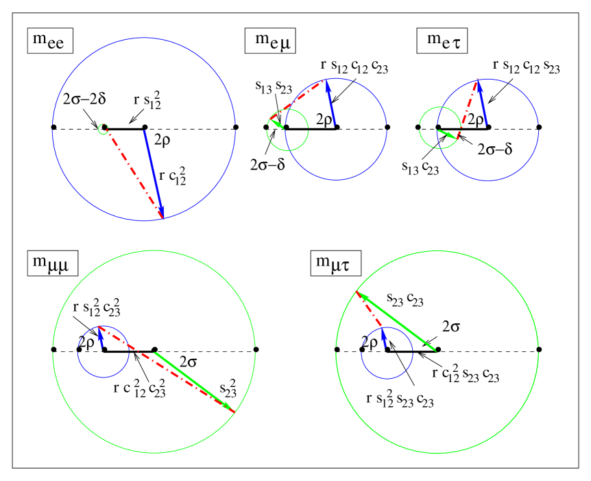
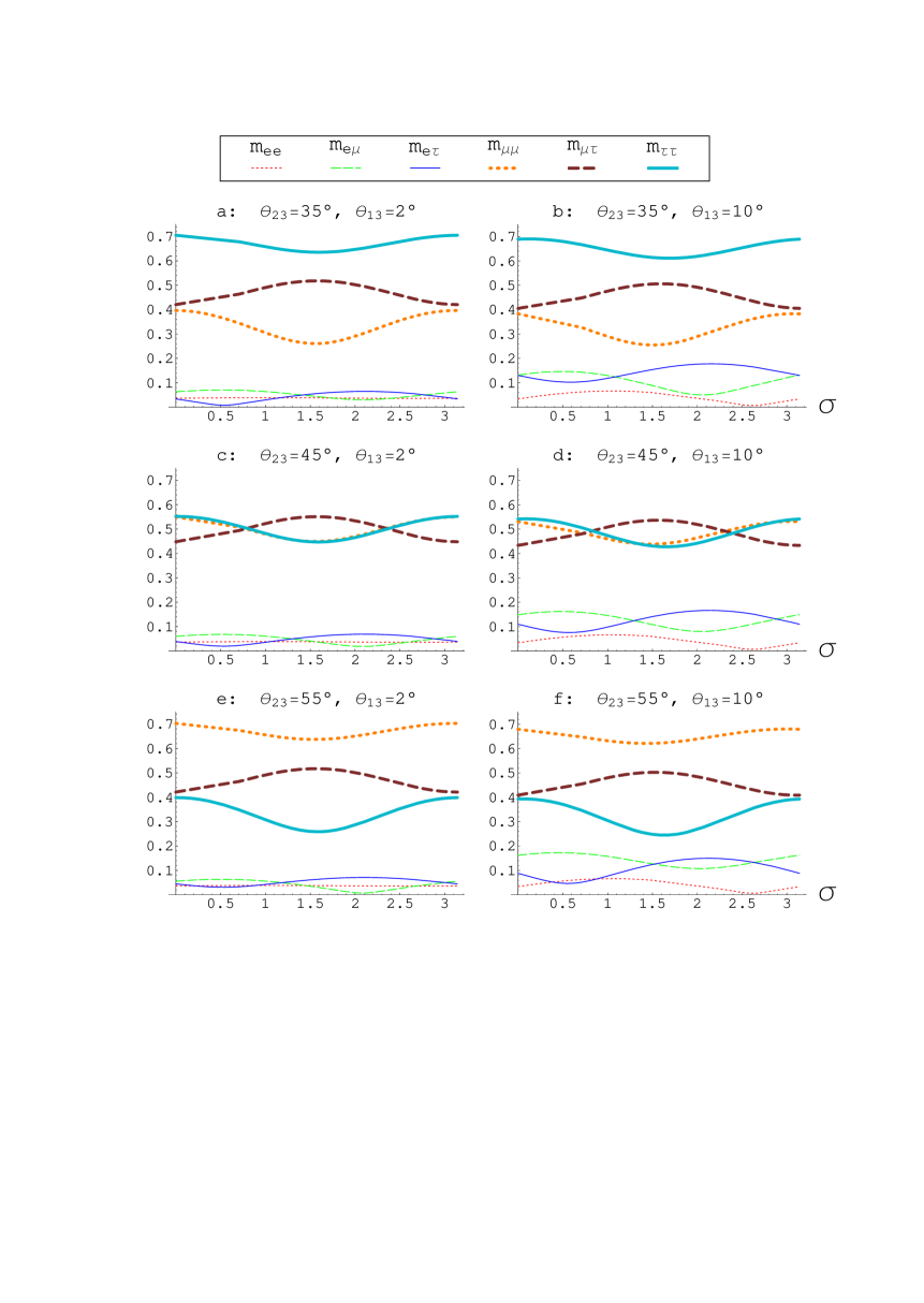
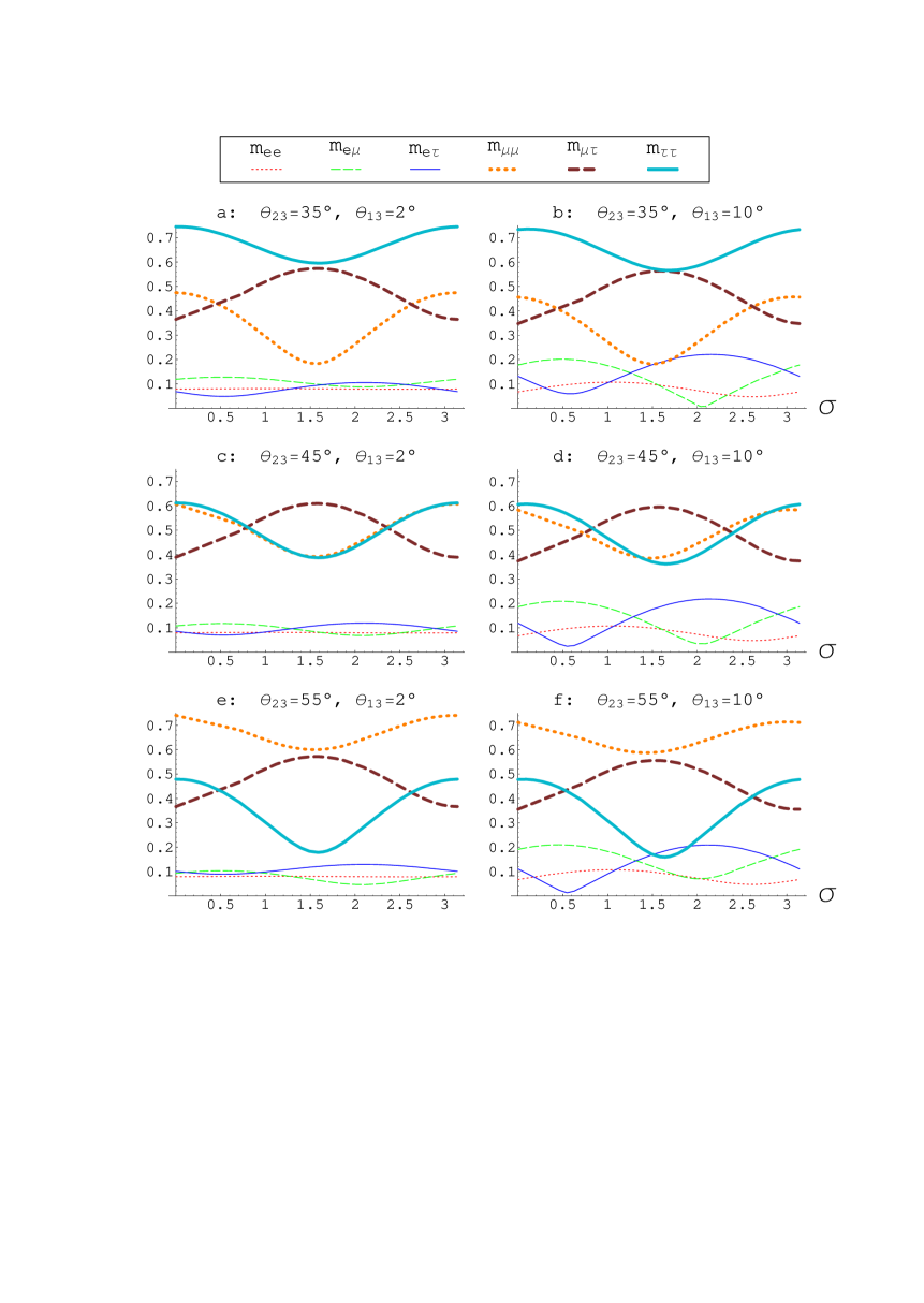
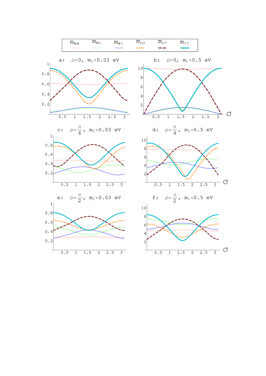
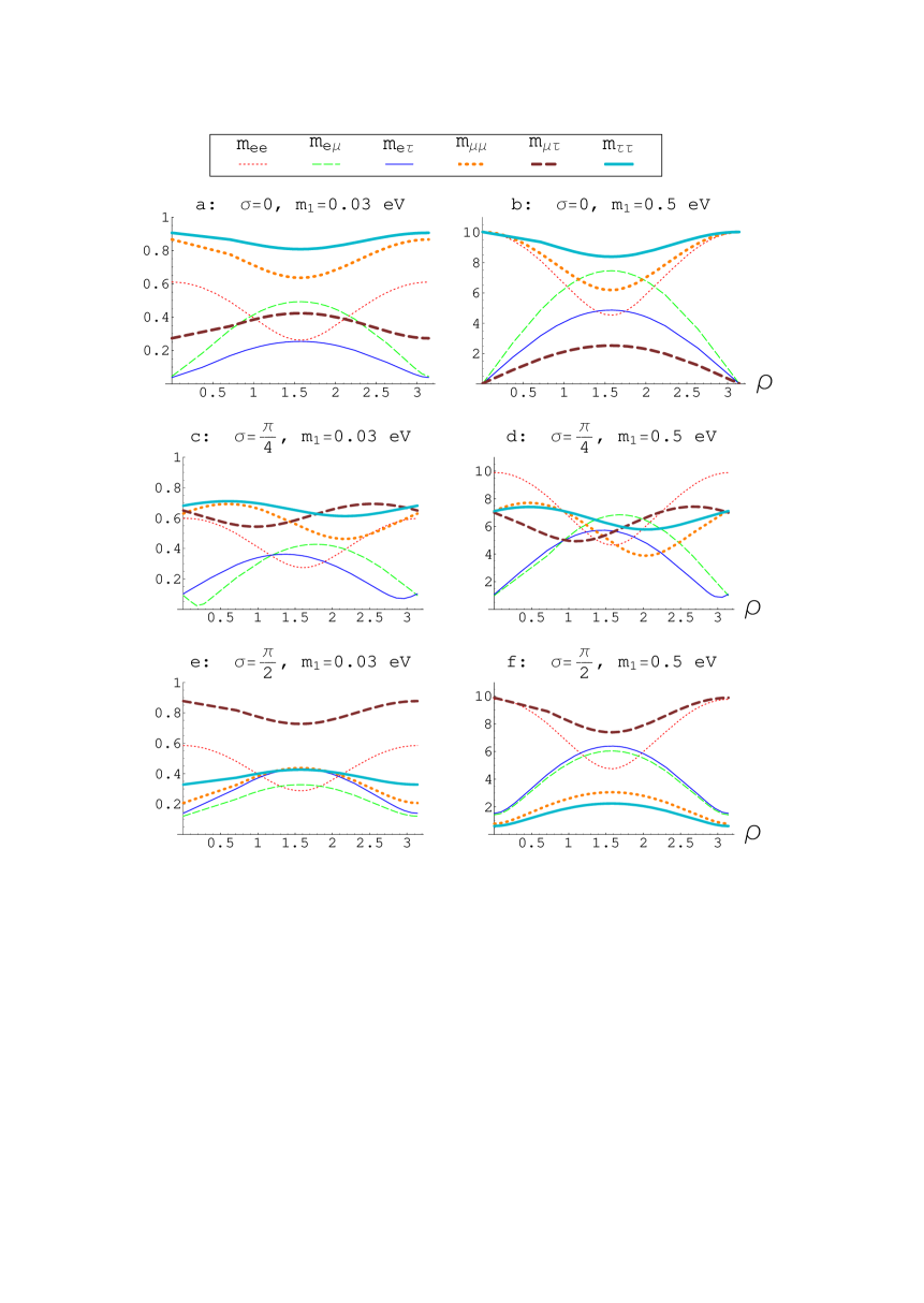
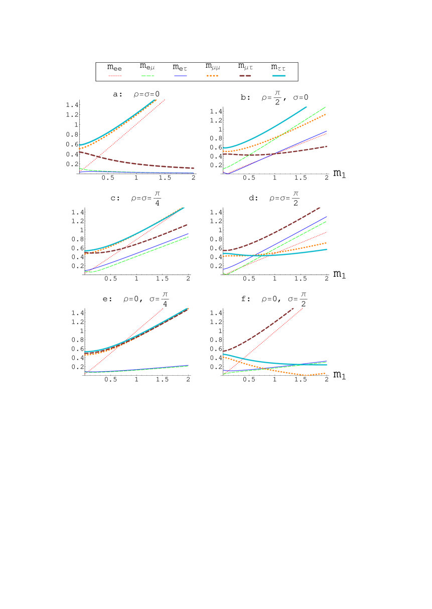
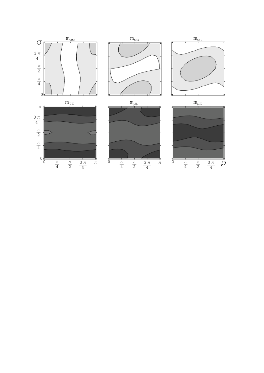
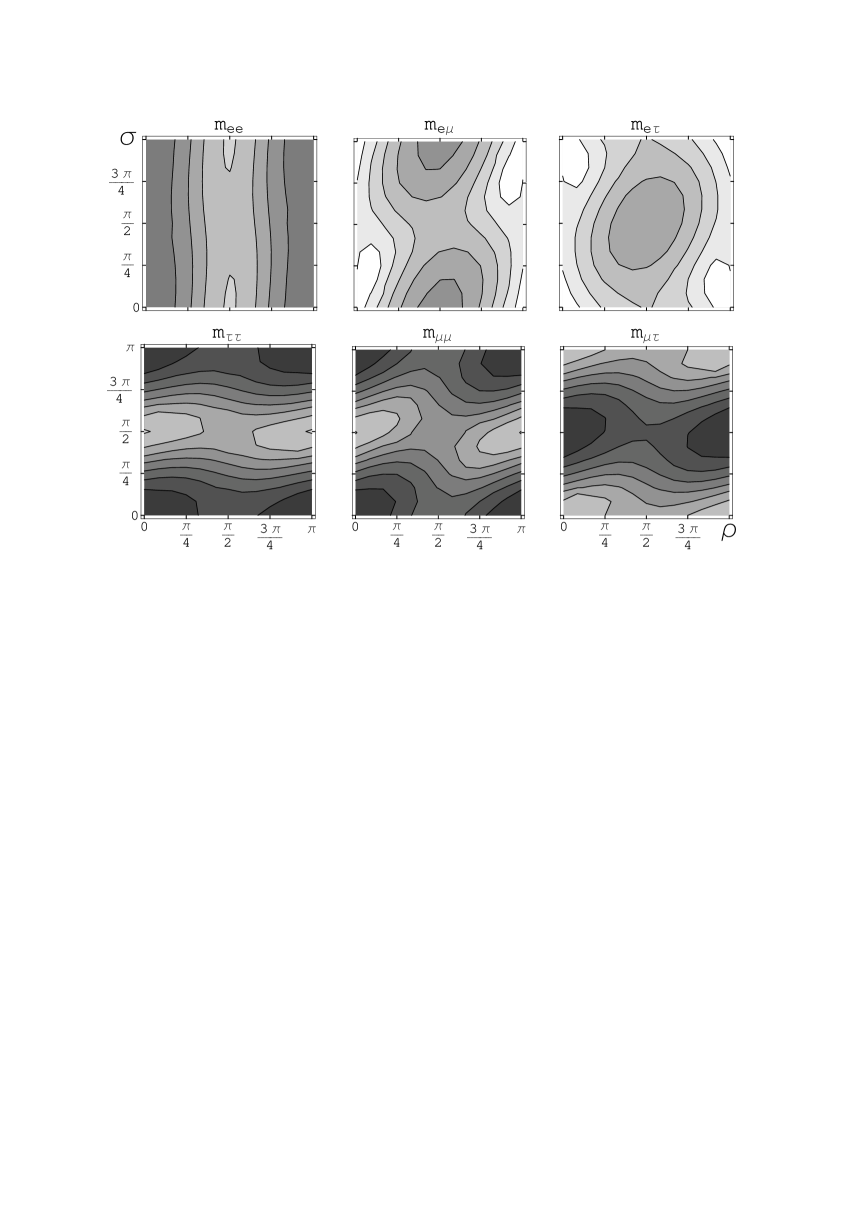
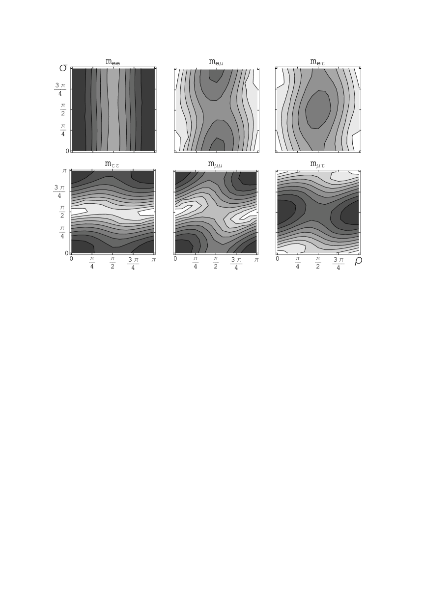
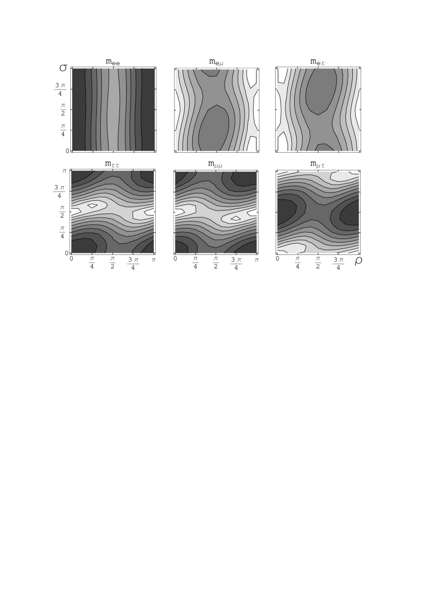
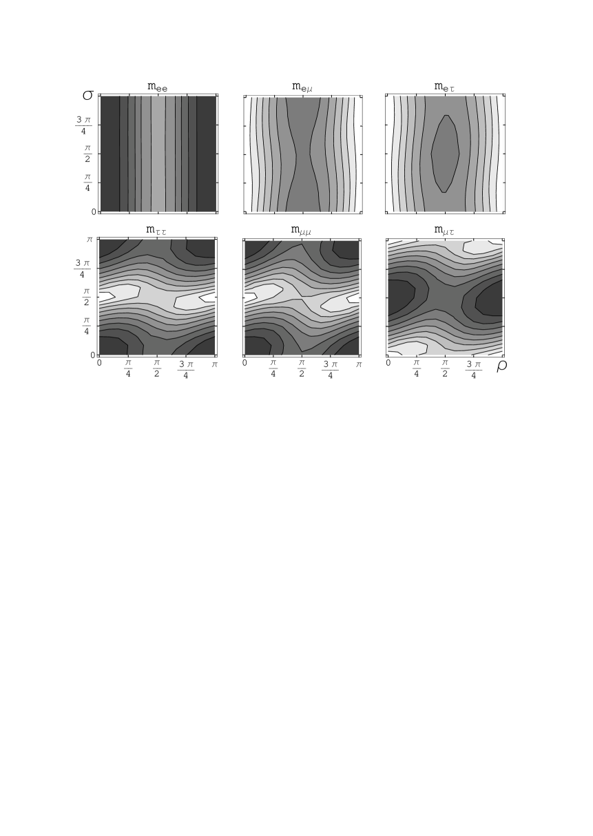
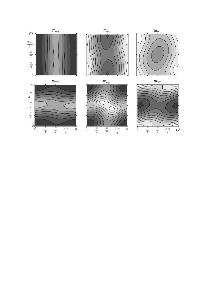
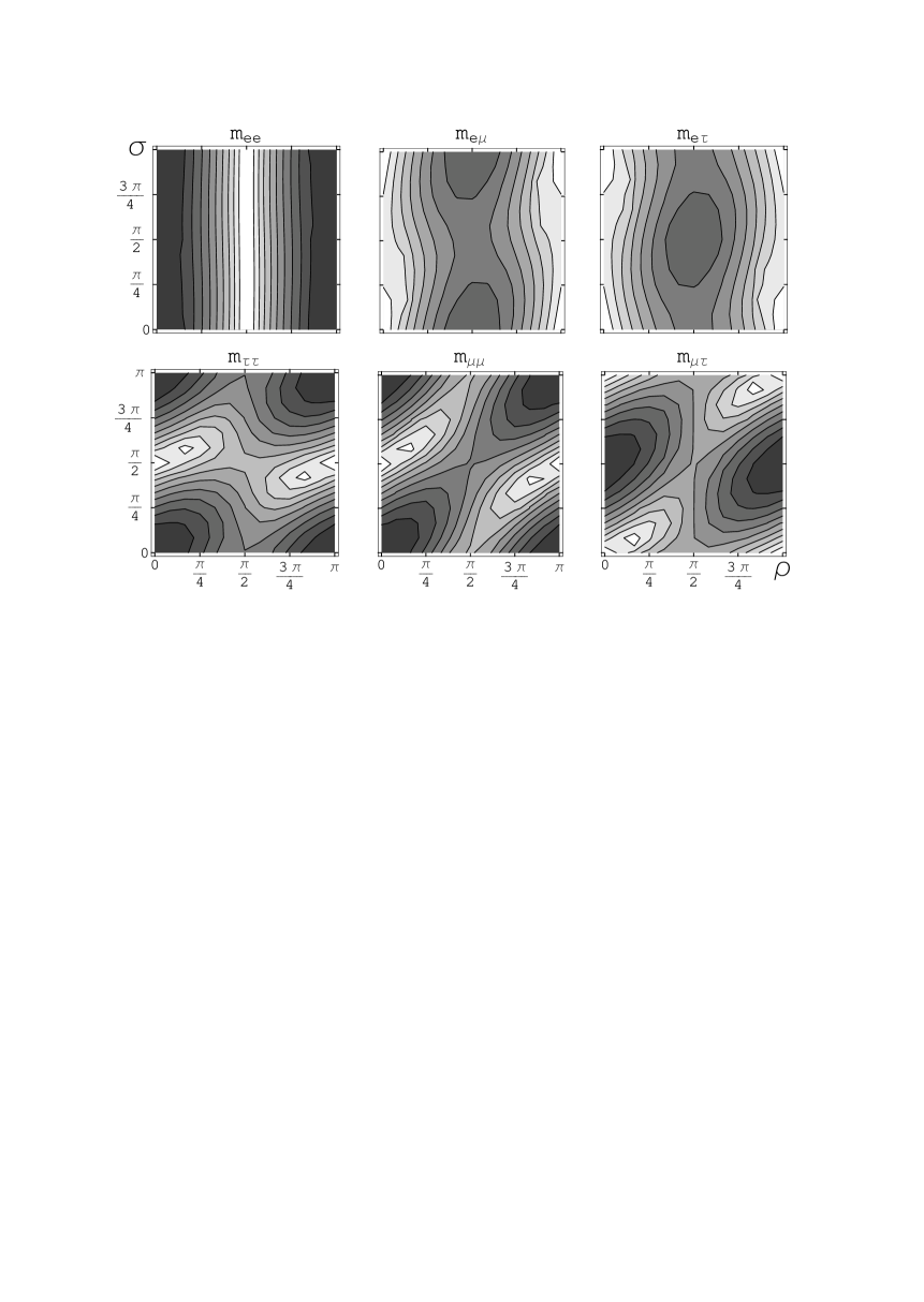
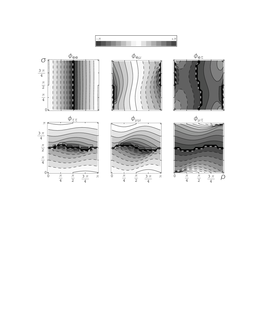
Appendix: Analytic expressions for matrix elements
For convenience of the reader we present here explicit expressions for the neutrino mass matrix elements in flavor basis, (), as functions of the mass eigenvalues , of the mixing angles and of the CP violating phases (see (4)).
Denoting and , we get the following expressions for the matrix elements, as sums of three terms corresponding to the three mass eigenstates:
| (A.1) |
| (A.2) |
| (A.3) |
| (A.4) |
| (A.5) |
| (A.6) |
It is convenient to use also a representation of the matrix elements as series in powers of . Using the equations (A.1)-(A.6) and the definitions (32), we get:
| (A.7) |
where
| (A.8) |
We will use also another form for the matrix elements, which is obtained neglecting terms of the order . For the -block, we get:
| (A.9) |
where
| (A.10) |
Notice that the three different terms in the Eqs.(A.9) are contributions of the three masses , and . For the elements of the -row we get, up to an overall factor :
| (A.11) |
where
| (A.12) |
The -element can be written as
| (A.13) |
It does not depend on the angle .
References
- [1] Y. Fukuda et al. [SuperKamiokande Collaboration], Phys. Lett. B 467 (1999) 185 [hep-ex/9908049]; S. Fukuda et al. [Super-Kamiokande Collaboration], Phys. Rev. Lett. 85 (2000) 3999 [hep-ex/0009001]; T. Toshito [SuperKamiokande Collaboration], hep-ex/0105023.
- [2] S. Fukuda et al. [SuperKamiokande Collaboration], Phys. Rev. Lett. 86 (2001) 5651 [hep-ex/0103032]; Phys. Rev. Lett. 86 (2001) 5656 [hep-ex/0103033]; Super-Kamiokande Collaboration, hep-ex/0205075.
- [3] Q. R. Ahmad et al. [SNO Collaboration], Phys. Rev. Lett. 87 (2001) 071301 [nucl-ex/0106015]; Phys. Rev. Lett. 89 (2002) 011301 [nucl-ex/0204008]; Phys. Rev. Lett. 89 (2002) 011302 [nucl-ex/0204009].
- [4] M. Apollonio et al. [CHOOZ Collaboration], Phys. Lett. B 420 (1998) 397 [hep-ex/9711002]; Phys. Lett. B 466 (1999) 415 [hep-ex/9907037]. See also: F. Boehm et al., Phys. Rev. D 64 (2001) 112001 [hep-ex/0107009].
- [5] H. V. Klapdor-Kleingrothaus et al., Eur. Phys. J. A 12 (2001) 147 [hep-ph/0103062]; H. V. Klapdor-Kleingrothaus, hep-ph/0103074.
- [6] C. D. Froggatt and H. B. Nielsen, Nucl. Phys. B 147 (1979) 277.
- [7] E. Papageorgiu, Z. Phys. C 64 (1994) 509 [hep-ph/9405256]; P. Binetruy, S. Lavignac and P. Ramond, Nucl. Phys. B 477 (1996) 353 [hep-ph/9601243]; J. K. Elwood, N. Irges and P. Ramond, Phys. Rev. Lett. 81 (1998) 5064 [hep-ph/9807228]; G. Altarelli and F. Feruglio, Phys. Lett. B 451 (1999) 388 [hep-ph/9812475]; S. Lola and G. G. Ross, Nucl. Phys. B 553 (1999) 81 [hep-ph/9902283]; S. F. King, Nucl. Phys. B 576 (2000) 85 [hep-ph/9912492]; K. Choi, E. J. Chun, K. Hwang and W. Y. Song, Phys. Rev. D 64 (2001) 113013 [hep-ph/0107083].
- [8] G. Altarelli and F. Feruglio, Phys. Rept. 320 (1999) 295.
- [9] D. B. Kaplan and M. Schmaltz, Phys. Rev. D 49 (1994) 3741 [hep-ph/9311281]; M. Fukugita, M. Tanimoto and T. Yanagida, Phys. Rev. D 57 (1998) 4429 [hep-ph/9709388]; Z. Berezhiani and A. Rossi, JHEP 9903 (1999) 002 [hep-ph/9811447] and Nucl. Phys. Proc. Suppl. 101 (2001) 410 [hep-ph/0107054]; P. H. Frampton and A. Rasin, Phys. Lett. B 478 (2000) 424 [hep-ph/9910522].
- [10] H. Fritzsch and Z. z. Xing, Prog. Part. Nucl. Phys. 45 (2000) 1 [hep-ph/9912358].
- [11] S. M. Barr and I. Dorsner, Nucl. Phys. B 585 (2000) 79 [hep-ph/0003058].
- [12] R. Barbieri, L. J. Hall, D. R. Smith, A. Strumia and N. Weiner, JHEP 9812 (1998) 017 [hep-ph/9807235]; R. Barbieri, L. J. Hall and A. Strumia, Phys. Lett. B 445 (1999) 407 [hep-ph/9808333].
- [13] F. Vissani, JHEP 9811 (1998) 025 [hep-ph/9810435]; Phys. Lett. B 508 (2001) 79 [hep-ph/0102236]; hep-ph/0111373.
- [14] E. K. Akhmedov, Phys. Lett. B 467 (1999) 95 [hep-ph/9909217]; A. Abada and M. Losada, Nucl. Phys. B 585 (2000) 45 [hep-ph/9908352]; T. Hambye, hep-ph/0201307; H. V. Klapdor-Kleingrothaus and U. Sarkar, hep-ph/0202006.
- [15] J. Sato and T. Yanagida, Phys. Lett. B 493 (2000) 356 [hep-ph/0009205].
- [16] F. Feruglio, A. Strumia and F. Vissani, hep-ph/0201291.
- [17] P. H. Frampton, S. L. Glashow and D. Marfatia, hep-ph/0201008; Z. z. Xing, hep-ph/0201151.
- [18] H. Fritzsch and Z. Z. Xing, Phys. Lett. B 372 (1996) 265 [hep-ph/9509389]; G. C. Branco, M. N. Rebelo and J. I. Silva-Marcos, Phys. Rev. D 62 (2000) 073004 [hep-ph/9906368]; E. K. Akhmedov, G. C. Branco, F. R. Joaquim and J. I. Silva-Marcos, Phys. Lett. B 498 (2001) 237 [hep-ph/0008010]; K. Fukuura, T. Miura, E. Takasugi and M. Yoshimura, Phys. Rev. D 61 (2000) 073002 [hep-ph/9909415].
- [19] L. J. Hall, H. Murayama and N. Weiner, Phys. Rev. Lett. 84 (2000) 2572 [hep-ph/9911341]; N. Haba and H. Murayama, Phys. Rev. D 63 (2001) 053010 [hep-ph/0009174].
- [20] S. Lavignac, I. Masina and C. A. Savoy, hep-ph/0202086.
- [21] K. Zuber, hep-ph/0008080.
- [22] W. Rodejohann, Phys. Rev. D 62 (2000) 013011 [hep-ph/0003149].
- [23] A. Y. Smirnov, D. N. Spergel and J. N. Bahcall, Phys. Rev. D 49 (1994) 1389 [hep-ph/9305204]; B. Jegerlehner, F. Neubig and G. Raffelt, Phys. Rev. D 54 (1996) 1194 [astro-ph/9601111]; H. Minakata and H. Nunokawa, Phys. Lett. B 504 (2001) 301 [hep-ph/0010240]; C. Lunardini and A. Y. Smirnov, Nucl. Phys. B 616 (2001) 307 [hep-ph/0106149].
- [24] V. Barger, D. Marfatia and B. P. Wood, hep-ph/0202158.
- [25] V. Barger, D. Marfatia, K. Whisnant and B. P. Wood, Phys. Lett. B 537 (2002) 179 [hep-ph/0204253]; A. Bandyopadhyay, S. Choubey, S. Goswami and D. P. Roy, hep-ph/0204286; J. N. Bahcall, M. C. Gonzalez-Garcia and C. Pena-Garay, hep-ph/0204314; P. Aliani, V. Antonelli, R. Ferrari, M. Picariello and E. Torrente-Lujan, hep-ph/0205053; P. C. de Holanda and A. Y. Smirnov, hep-ph/0205241; A. Strumia, C. Cattadori, N. Ferrari and F. Vissani, hep-ph/0205261; G. L. Fogli, E. Lisi, A. Marrone, D. Montanino and A. Palazzo, hep-ph/0206162.
- [26] A. Piepke [KamLAND Collaboration], Nucl. Phys. Proc. Suppl. 91 (2001) 99; V. D. Barger, D. Marfatia and B. P. Wood, Phys. Lett. B 498 (2001) 53 [hep-ph/0011251]; A. de Gouvea and C. Pena-Garay, Phys. Rev. D 64 (2001) 113011 [hep-ph/0107186].
- [27] J. Bonn et al., Nucl. Phys. Proc. Suppl. 91 (2001) 273.
- [28] C. E. Aalseth et al., hep-ex/0202026.
- [29] H. V. Klapdor-Kleingrothaus, A. Dietz, H. L. Harney and I. V. Krivosheina, Mod. Phys. Lett. A 16 (2001) 2409 [hep-ph/0201231].
- [30] C. E. Aalseth et al., hep-ex/0202018; H. V. Klapdor-Kleingrothaus, hep-ph/0205228; H. L. Harney, hep-ph/0205293.
- [31] H. V. Klapdor-Kleingrothaus, H. Pas and A. Y. Smirnov, Phys. Rev. D 63 (2001) 073005 [hep-ph/0003219].
- [32] F. Vissani, hep-ph/9708483.
- [33] H. Nishiura, K. Matsuda and T. Fukuyama, Mod. Phys. Lett. A 14 (1999) 433 [hep-ph/9809556].
- [34] F. Vissani, JHEP 9906 (1999) 022 [hep-ph/9906525].
- [35] H. Minakata and O. Yasuda, Phys. Rev. D 56 (1997) 1692 [hep-ph/9609276]. W. Rodejohann, Nucl. Phys. B 597 (2001) 110 [hep-ph/0008044].
- [36] A. Osipowicz et al. [KATRIN Collaboration], hep-ex/0109033.
- [37] M. Frigerio and A. Yu. Smirnov, in preparation.
- [38] K. S. Babu and S. M. Barr, Phys. Lett. B 525 (2002) 289 [hep-ph/0111215].
- [39] K. S. Babu, C. N. Leung and J. Pantaleone, Phys. Lett. B 319 (1993) 191 [hep-ph/9309223]; J. R. Ellis and S. Lola, Phys. Lett. B 458 (1999) 310 [hep-ph/9904279]; J. A. Casas, J. R. Espinosa, A. Ibarra and I. Navarro, Nucl. Phys. B 573 (2000) 652 [hep-ph/9910420]; S. Antusch, M. Drees, J. Kersten, M. Lindner and M. Ratz, Phys. Lett. B 519 (2001) 238 [hep-ph/0108005]; P. H. Chankowski and S. Pokorski, hep-ph/0110249.