The Snowmass Points and Slopes: Benchmarks for SUSY Searches

Abstract

The “Snowmass Points and Slopes” (SPS) are a set of benchmark points and parameter lines in the MSSM parameter space corresponding to different scenarios in the search for Supersymmetry at present and future experiments. This set of benchmarks was agreed upon at the 2001 “Snowmass Workshop on the Future of Particle Physics” as a consensus based on different existing proposals.

I Why benchmarks — which benchmarks?

In the unconstrained version of the Minimal Supersymmetric extension of the Standard Model (MSSM) no particular Supersymmetry (SUSY) breaking mechanism is assumed, but rather a parameterization of all possible soft SUSY breaking terms is used. This leads to more than a hundred parameters (masses, mixing angles, phases) in this model in addition to the ones of the Standard Model. The currently most popular SUSY breaking mechanisms are minimal supergravity (mSUGRA) msugra , gauge-mediated SUSY breaking (GMSB) gmsb , and anomaly-mediated SUSY breaking (AMSB) amsb . In these scenarios SUSY breaking happens in a hidden sector and is mediated to the visible sector (i.e. the MSSM) in different ways: via gravitational interactions in the mSUGRA scenario, via gauge interactions in the GMSB scenario, and via the super-Weyl anomaly in the AMSB scenario. Assuming one of these SUSY breaking mechanisms leads to a drastic reduction of the number of parameters compared to the MSSM case. The mSUGRA scenario is characterized by four parameters and a sign, the scalar mass parameter $m_{0}$, the gaugino mass parameter $m_{1/2}$, the trilinear coupling $A_{0}$, the ratio of the Higgs vacuum expectation values, $\tan\beta$, and the sign of the supersymmetric Higgs mass parameter, $\mu$. The parameters of the (minimal) GMSB scenario are the messenger mass $M_{\rm mes}$, the messenger index $N_{\rm mes}$, the universal soft SUSY breaking mass scale felt by the low-energy sector, $\Lambda$, as well as $\tan\beta$ and $\mathrm{sign}(\mu)$. The (minimal) AMSB scenario has the parameters $m_{\rm aux}$, which sets the overall scale of the SUSY particle masses (given by the vacuum expectation value of the auxiliary field in the supergravity multiplet), $\tan\beta$, $\mathrm{sign}(\mu)$, and $m_{0}$, where the latter is a phenomenological parameter introduced in order to keep the squares of slepton masses positive. The mass spectra of the SUSY particles in these scenarios are obtained via renormalization group running from the scale of the high-energy parameters of the SUSY-breaking scenario to the weak scale. The low-energy parameters obtained in this way are then used as input for calculating the predictions for the production cross sections and for the decay branching ratios of the SUSY particles.

While a detailed scanning over the more-than-hundred-dimensional parameter space of the MSSM is clearly not practicable, even a sampling of the three- or four-dimensional parameter space of the above-mentioned SUSY breaking scenarios is beyond the present capabilities for phenomenological studies, in particular when it comes to simulating experimental signatures within the detectors. For this reason one often resorts to specific benchmark scenarios, i.e. one studies only specific parameter points or at best samples a one-dimensional parameter space (the latter is sometimes called a model line modelline ), which exhibit specific characteristics of the MSSM parameter space. Benchmark scenarios of this kind are often used, for instance, for studying the performance of different experiments at the same collider. Similarly, detailed experimental simulations of sparticle production with identical MSSM parameters in the framework of different colliders can be very helpful for developing strategies for combining pieces of information obtained at different machines.

The question of which parameter choices are useful as benchmark scenarios depends on the purpose of the actual investigation. If one is interested, for instance, in setting exclusion limits on the SUSY parameter space from the non-observation of SUSY signals at the experiments performed up to now, it is useful to use a benchmark scenario which gives rise to “conservative” exclusion bounds. An example of a benchmark scenario of this kind is the $m_{\mathrm{h}}^{\mathrm{max}}$-scenario lephiggsbenchmarks used for the Higgs search at LEP lepbench and the Tevatron tevbench . It gives rise to maximal values of the lightest ${\cal CP}$-even Higgs-boson mass (for fixed values of the top-quark mass and the SUSY scale) and thus allows one to set conservative bounds on $\tan\beta$ and $M_{\mathrm{A}}$ (the mass of the ${\cal CP}$-odd Higgs boson) tbexcl . Another application of benchmark scenarios is to study “typical” experimental signatures of SUSY models and to investigate the experimental sensitivities and the achievable experimental precisions for these cases. For this purpose it seems reasonable to choose “typical” (a notion which is of course difficult to define) and theoretically well motivated parameters of certain SUSY-breaking scenarios. Examples of this kind are the benchmark scenarios used so far for investigating SUSY searches at the LHC benchsnow96 ; tdratlcms , the Tevatron tevsugra and at a future Linear Collider teslatdr . As a further possible goal of benchmark scenarios, one can choose them so that they account for a wide variety of SUSY phenomenology. For this purpose, one could for instance analyse SUSY with R-parity breaking, investigate effects of non-vanishing ${\cal CP}$ phases, or inspect non-minimal SUSY models. In this context it can also be useful to consider “pathological” regions of parameter space or “worst-case” scenarios. Examples for this are the “large-$|\mu|$ scenario” for the Higgs search at LEP lephiggsbenchmarks and the Tevatron hadhiggsbenchmarks , for which the decay $h\to b\bar{b}$ can be significantly suppressed, or a scenario where the Higgs boson has a large branching fraction into invisible decay modes at the LHC (see e.g. Ref. fawzi ).

A related issue concerning the definition of appropriate benchmarks is whether a benchmark scenario chosen for investigating physics at a certain experiment or for testing a certain sector of the theory should be compatible with additional information from other experiments (or concerning other sectors of the theory). This refers in particular to constraints from cosmology (by demanding that SUSY should give rise to an acceptable dark matter density cdm ) and low-energy measurements such as the rate for $b\to s\gamma$ bsg and the anomalous magnetic moment of the muon, $g_{\mu}-2$ gminus2 (see Ref. gminus2th for the updated SM prediction for $g_{\mu}-2$). On the one hand, applying constraints of this kind gives rise to “more realistic” benchmark scenarios. On the other hand, one relies in this way on further assumptions (and has to take account of experimental and theoretical uncertainties related to these additional constraints), and it could eventually turn out that one has inappropriately narrowed down the range of possibilities by applying these constraints. This applies in particular if slight modifications of the SUSY breaking scenarios are allowed that have a minor impact on collider phenomenology but could significantly alter the bounds from cosmology and low-energy experiments. For instance, the presence of small flavor mixing terms in the SUSY Lagrangian could severely affect the prediction for BR($b\to s\gamma$), while allowing a small amount of R-parity violation in the model would strongly affect the constraints from dark matter relic abundance while leaving collider phenomenology essentially unchanged. In the context of additional constraints one also has to decide on the level of fine-tuning of parameters (as a measure to distinguish between “more natural” and “less natural” parameter choices) one should tolerate in a benchmark scenario.

The extent to which additional constraints of this kind should be applied to possible benchmark scenarios is related to the actual purpose of the benchmark scenario. For setting exclusion bounds in a particular sector (e.g. the Higgs sector) it seems preferable to apply constraints only from this sector. Similarly, relaxing additional constraints should also be appropriate for the investigation of “worst-case” scenarios and for studying possible collider signatures. Making use of all available information, on the other hand, would be preferable when testing whether a certain model is actually the “correct” theory.

From the above discussion it should be obvious that it is not possible to define a single set of benchmark scenarios that will serve all purposes. The usefulness of a particular scenario will always depend on which sector of the theory (e.g. the Higgs or the chargino/neutralino sector) and which physics issue is investigated (exclusion limits or “typical” scenarios at colliders, dark matter searches, etc.). Accordingly, a comparison of the physics potential of different experiments on the basis of specific benchmark scenarios is necessarily very difficult.

The need for reconsidering the issue of defining appropriate benchmarks for SUSY searches at the next generation of colliders becomes apparent from the fact that the exclusion bounds in the Higgs sector of the MSSM obtained from the Higgs search at LEP rule out several of the benchmark points used up to now for studies of SUSY phenomenology at future colliders. Accordingly, after the termination of the LEP program several proposals for new benchmark scenarios for SUSY searches have been made by different groups.

The “Snowmass Points and Slopes” (SPS), which we will discuss in the following, are a set of benchmark scenarios which arose from the 2001 “Snowmass Workshop on the Future of Particle Physics” as a consensus based on different proposals recently made by various groups. The SPS consist of model lines (“slopes”), i.e. continuous sets of parameters depending on one dimensionful parameter (see below) and specific benchmark points, where each model line goes through one of the benchmark points. The SPS should be regarded as a recommendation for future studies of SUSY phenomenology, but of course are not meant as an exclusive and for all purposes sufficient collection of SUSY models. They mainly focus on “typical” scenarios within the three currently most prominent SUSY-breaking mechanisms, i.e. mSUGRA, GMSB and AMSB. Furthermore they contain examples of “more extreme” scenarios, e.g. a “focus point” scenario focuspoint with a rather heavy SUSY spectrum, indicating in this way different possibilities for SUSY phenomenology that can be realized within the most commonly used SUSY breaking scenarios.

II Recent proposals for SUSY benchmarks

Before discussing the SPS in detail, we first briefly review some recent proposals for SUSY benchmark scenarios. In Ref. BDEGMOPW , henceforth denoted as BDEGMOPW, a set of 13 parameter points in the CMSSM (i.e. the mSUGRA) scenario has been proposed according to the constraints arising from demanding that the lightest supersymmetric particle (LSP) should give rise to a cosmologically acceptable dark matter relic abundance: five points were chosen in the “bulk” of the cosmological region, four points along the “coannihilation tail” (where a rapid coannihilation takes place between the LSP and the (almost mass degenerate) next-to-lightest SUSY particle (NSLP), which is usually the lighter $\tilde{\tau}$), two points were chosen in rapid-annihilation “funnels” (where an increased annihilation cross section of the LSP results from poles due to the heavier neutral MSSM Higgs bosons $H$ and $A$), and two points in the “focus-point” region (where the annihilation cross section of the LSP is enhanced due to a sizable higgsino component). The BDEGMOPW points are all taken for the value of the trilinear coupling $A_{0}=0$, i.e. the parameters that are varied are $m_{0}$, $m_{1/2}$, $\tan\beta$ and $\mathrm{sign}(\mu)$. They were in particular chosen to span a wide range of $\tan\beta$ values.

The constraints from the LEP Higgs search and the measurement of $b\to s\gamma$ have been imposed for all of the BDEGMOPW points, while the $g_{\mu}-2$ constraint was not enforced (at the time of the proposal of the BDEGMOPW points only the points in the “bulk” of the cosmological region were in agreement with the $g_{\mu}-2$ constraint, while taking into account the updated SM value for $g_{\mu}-2$ gminus2th all but one of the BDEGMOPW points satisfy the $g_{\mu}-2$ constraint at the $2\sigma$ level). The “bulk” of the cosmological region and the low-mass portion of the “focus point” region are favored if fine-tuning constraints are applied.

The “Points d’Aix” is a different set of benchmark points, which were proposed in the framework of the Euro-GDR SUSY Workshop aix . It consists of eleven benchmark points, out of which six belong to the mSUGRA scenario, four to the GMSB scenario and one to the AMSB scenario. The constraints from the LEP Higgs search and the electroweak precision data have been applied to all benchmark points. For the mSUGRA points further constraints from $b\to s\gamma$, $g_{\mu}-2$, and cosmology have been used, while for the GMSB points the constraints from $b\to s\gamma$ and $g_{\mu}-2$ have been taken into account. No further constraints have been applied for the AMSB point.

In Ref. modelline a set of eight “model lines” in the mSUGRA, GMSB and AMSB scenarios has been proposed. The model lines were designed for studying typical SUSY signatures as a function of the SUSY scale. Accordingly, each model line depends on one dimensionful parameter, which sets the overall SUSY scale, while $\tan\beta$ and $\mathrm{sign}(\mu)$ are kept fixed for each model line. The other dimensionful parameters in each SUSY-breaking scenario are taken to scale linearly with the parameter being varied along the model line. Since the main focus in this approach lies in investigating typical SUSY signatures, neither constraints from Higgs and SUSY particle searches nor from $b\to s\gamma$, $g_{\mu}-2$, or cosmology were applied. Four of the model lines refer to the mSUGRA scenario, one corresponds to an mSUGRA-like scenario with non-unified gaugino masses, two model lines are realizations of the GMSB scenario, and one of the AMSB scenario.

III The Snowmass Points and Slopes (SPS)

The Snowmass Points and Slopes (SPS) are based on an attempt to merge the features of the above proposals for different benchmark scenarios into a subset of commonly accepted benchmark scenarios. They consist of benchmark points and model lines (“slopes”). There are ten benchmark points, from which six correspond to an mSUGRA scenario, one is an mSUGRA-like scenario with non-unified gaugino masses, two refer to the GMSB scenario, and one to the AMSB scenario. Seven of these benchmark points are attached to model lines, while the remaining three are supplied as isolated points (one could of course also define model lines going through these points, but since studying a model line will require more effort than studying a single point, it seemed unnecessary to equip every chosen benchmark point with a model line). In studying the benchmark scenarios the model lines should prove useful in performing more general analyses of typical SUSY signatures, while the specific points indicated on the lines are proposed to be chosen as the first sample points for very detailed (and thus time-consuming) analyses. The concept of a model line means of course that more than just one point should be studied on each line. Results along the model lines can often then be roughly estimated by interpolation.

An important aspect in the philosophy behind the benchmark scenarios is that the low-energy MSSM parameters should be regarded as the actual benchmark rather than the high-energy input parameters $m_{0}$, $m_{1/2}$, etc. Thus, specifying the benchmark scenarios in terms of the latter parameters is merely understood as an abbreviation for the low-energy phenomenology.

The relevant low-energy parameters are the soft SUSY-breaking parameters in the diagonal entries of the sfermion mass matrices (using the notation of the first generation),

$$M_{\tilde{q}1_{L}},M_{\tilde{d}_{R}},M_{\tilde{u}_{R}},M_{\tilde{e}_{L}},M_{\tilde{e}_{R}},$$ (1)

and analogously for the other two generations, as well as

$$A_{t},A_{b},A_{\tau},\ldots,M_{1},M_{2},M_{\tilde{g}},\mu,M_{A},\tan\beta,$$ (2)

where the $A_{i}$ are the trilinear couplings, $M_{1}$, $M_{2}$ are the electroweak gaugino mass parameters, $M_{\tilde{g}}$ is the gluino mass, and $M_{A}$ is the mass of the ${\cal CP}$-odd neutral Higgs boson.

Our convention for the sign of $\mu$ is such that the neutralino and chargino mass matrices have the following form

$${\bf M}_{\widetilde{\chi}^{0}}=\pmatrix{M_{1}&0&-g^{\prime}v_{d}/\sqrt{2}&g^{\prime}v_{u}/\sqrt{2}\cr 0&M_{2}&gv_{d}/\sqrt{2}&-gv_{u}/\sqrt{2}\cr-g^{\prime}v_{d}/\sqrt{2}&gv_{d}/\sqrt{2}&0&-\mu\cr g^{\prime}v_{u}/\sqrt{2}&-gv_{u}/\sqrt{2}&-\mu&0},\qquad{\bf M}_{\widetilde{\chi}^{\pm}}=\pmatrix{M_{2}&gv_{u}\cr gv_{d}&\mu}.$$ (3)

In order to relate the high-energy input parameters to the corresponding low-energy MSSM parameters specified in eqs. (1), (2), a certain standard has to be chosen. It was agreed that this standard should be version 7.58 of the program ISAJET isajet . It should be stressed at this point that the definition of this standard contains a certain degree of arbitrariness. In particular, for the purpose of defining certain spectra as benchmarks, the issue of how accurately high-energy input parameters can be related (via renormalization group running) to the corresponding low-energy parameters in different programs (e.g. ISAJET, SUSYGEN susygen , SUSPECT suspect , SOFTSUSY softsusy , SUITY suity , BMPZ bmpz , etc.) is of minor importance and therefore has not been addressed in the context of the SPS. Once a standard has been defined for relating the high-energy input parameters to the low-energy MSSM parameters, the way the latter were obtained and the precise values of the high-energy input parameters are no longer relevant.

In order to perform the analysis of the SPS benchmark scenarios with a program like PYTHIA pythia or HERWIG herwig , it is the easiest to use the output of ISAJET 7.58 for the parameters specified in eqs. (1), (2) directly as input for these programs. Alternatively, if one prefers to use the high-energy parameters $m_{0}$, $m_{1/2}$, etc. as input in a program like SUSYGEN, one should make sure that the low-energy parameters of eq. (1), (2) agree within reasonable precision with the actual benchmark values. If using the input values $m_{0}$, $m_{1/2}$, etc. given below in a different program leads to a significant deviation in the parameters of eqs. (1), (2), these high-energy input parameters should be adapted such that the low-energy parameters are brought into approximate agreement. Since the low-energy MSSM parameters corresponding to ISAJET 7.58 have been frozen as benchmarks by definition, an appropriate adaptation will also be necessary for upgrades of ISAJET beyond version 7.58.

While it appears to be reasonable to fix certain sets of low-energy MSSM parameters as benchmarks by definition (which in principle could have been done without resorting at all to scenarios like mSUGRA, GMSB and AMSB), it on the other hand doesn’t seem justified to freeze the particle spectra, branching ratios, etc. obtained from these low-energy MSSM parameters as well. It is obvious that no single program exists which represents the current “state of the art” for computing all particle masses and branching ratios, and it should of course also be possible to take future improvements into account. The level of accuracy of the theoretical predictions presently implemented in a multi-purpose program like ISAJET will not always be sufficient. This refers in particular to the MSSM Higgs sector, where it will usually be preferable to resort to dedicated programs like FeynHiggs feynhiggs , subhpole subh , or HDECAY hdecay for cross-checking.

For the evaluation of the mass spectra and decay branching ratios from the MSSM benchmark parameters one should therefore choose an appropriate program according to the specific requirements of the analysis that is being performed. If detailed comparisons between different experiments or different colliders are carried out, it would clearly be advantageous to use the same results for the mass spectra and the branching ratios.

Concerning the compatibility with external constraints, all benchmark points corresponding to the mSUGRA scenario give rise to a cosmologically acceptable dark matter relic abundance (according to the bounds applied in Refs. BDEGMOPW ; aix , i.e. $0.1\leq\Omega_{\chi}h^{2}\leq 0.3$ for the BDEGMOPW points and $0.025<\Omega_{\chi}h^{2}<0.5$ for the “Points d’Aix”). In all SPS scenarios $\mu>0$ has been chosen. Within mSUGRA models, positive values of $\mu$ lead to values of $b\to s\gamma$ and $g_{\mu}-2$ which, within our present theoretical understanding, are consistent with the current experimental values of these quantities over a wide parameter range. While there is in general a slight preference for $\mu>0$, one certainly cannot regard the case $\mu<0$ as being experimentally excluded at present. We have nevertheless restricted to scenarios with positive $\mu$, since choosing $\mu$ negative does not lead to new characteristic experimental signatures as compared to the case with $\mu>0$.

Taking the updated SM value for $g_{\mu}-2$ gminus2th into account, the allowed 2-$\sigma$ range for SUSY contributions to $a_{\mu}\equiv(g_{\mu}-2)/2$ is currently $-6\times 10^{-10}<a_{\mu}<58\times 10^{-10}$. Accordingly, at present no upper bound on the SUSY masses can be inferred from the $g_{\mu}-2$ constraint, but only a rather mild lower bound. For the constraint from $b\to s\gamma$, the bound $2.33\times 10^{-4}<\mbox{BR}(b\to s\gamma)<4.15\times 10^{-4}$ has been used for the BDEGMOPW mSUGRA points BDEGMOPW , while $2\times 10^{-4}<\mbox{BR}(b\to s\gamma)<5\times 10^{-4}$ has been used for the mSUGRA and GMSB points of the “Points d’Aix” aix .

The main qualitative difference between the SPS (and also the recent proposals for post-LEP benchmarks in Refs. modelline ; BDEGMOPW ; aix ) and the benchmarks used so far for investigating SUSY searches at the LHC, the Tevatron and a future Linear Collider is that scenarios with small values of $\tan\beta$, i.e. $\tan\beta\;\raisebox{-3.00003pt}{$\stackrel{{\scriptstyle\displaystyle<}}{{\sim}}$}\;3$, are disfavored as a result of the Higgs exclusion bounds obtained at LEP. Consequently, there is more focus now on scenarios with larger values of $\tan\beta$ than in previous studies. Concerning the SUSY phenomenology, intermediate and large values of $\tan\beta$, $\tan\beta\;\raisebox{-3.00003pt}{$\stackrel{{\scriptstyle\displaystyle>}}{{\sim}}$}\;5$, have the important consequence that there is in general a non-negligible mixing between the two staus (and an even more pronounced mixing in the sbottom sector), leading to a significant mass splitting between the two staus so that the lighter stau becomes the lightest slepton. Neutralinos and charginos therefore decay predominantly into staus and taus, which is experimentally more challenging than the dilepton signal resulting for instance from the decay of the second lightest neutralino into the lightest neutralino and a pair of leptons of the first or the second generation.

Large values of $\tan\beta$ can furthermore have important consequences for the phenomenology in the Higgs sector, as the couplings of the heavy Higgs bosons $H$, $A$ to down-type fermions are in general enhanced. For sizable values of $\mu$ and $m_{\tilde{g}}$ the $hb\bar{b}$ coupling receives large radiative corrections from gluino loop corrections, which in particular affect the branching ratio BR($h\to\tau^{+}\tau^{-}$).

In the following we list the SPS benchmark scenarios. The value of the top-quark mass in all cases is chosen to be $m_{\mathrm{t}}=175$ GeV.

       SPS 1a                                                                 SPS 1b   
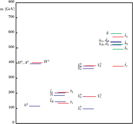
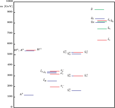
       SPS 2                                                                 SPS 3
  

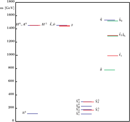
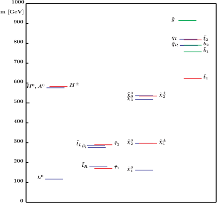
Figure 1: The SUSY particle spectra for the benchmark points corresponding to SPS 1a, SPS 1b, SPS 2 and SPS 3 as obtained with ISAJET 7.58 (see Ref. ulinabil ).

       SPS 4                                                                 SPS 5   
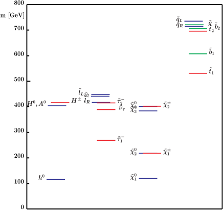
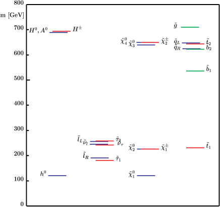
       SPS 6                                                                 SPS 7
  

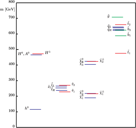
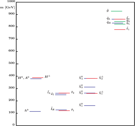
Figure 2: The SUSY particle spectra for the benchmark points corresponding to SPS 4, SPS 5, SPS 6 and SPS 7 as obtained with ISAJET 7.58 (see Ref. ulinabil ).

       SPS 8                                                                 SPS 9   

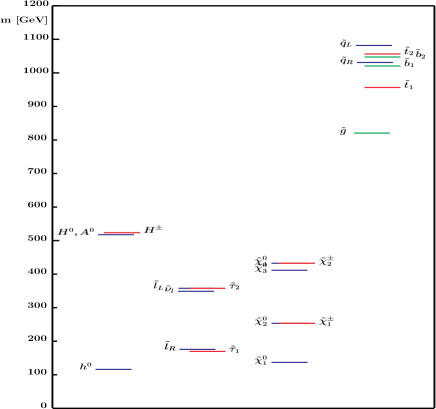
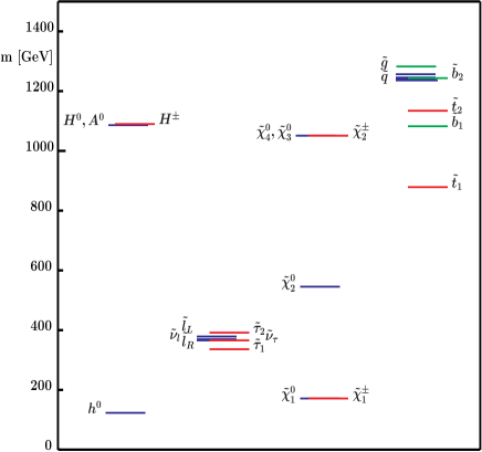
Figure 3: The SUSY particle spectra for the benchmark points corresponding to SPS 8 and SPS 9 as obtained with ISAJET 7.58 (see Ref. ulinabil ).

SPS 1: “typical” mSUGRA scenario

This scenario consists of a “typical” mSUGRA point with an intermediate value of $\tan\beta$ and a model line attached to it (SPS 1a) and of a “typical” mSUGRA point with relatively high $\tan\beta$ (SPS 1b). The two-points lie in the “bulk” of the cosmological region. For the collider phenomenology in particular the $\tau$-rich neutralino and chargino decays are important.

SPS 1a:
Point:

$$m_{0}=100\,\mathrm{GeV},\quad m_{1/2}=250\,\mathrm{GeV},\quad A_{0}=-100\,\mathrm{GeV},\quad\tan\beta=10,\quad\mu>0.$$

Slope:

$$m_{0}=-A_{0}=0.4\,m_{1/2},\quad m_{1/2}\mbox{ varies}.$$

The point is similar to BDEGMOPW point B. The slope equals model line A modelline .
SPS 1b:
Point:

$$m_{0}=200\,\mathrm{GeV},\quad m_{1/2}=400\,\mathrm{GeV},\quad A_{0}=0,\quad\tan\beta=30,\quad\mu>0.$$

This point is the mSUGRA point 6 of the “Points d’Aix”.

SPS 2: “focus point” scenario in mSUGRA

The benchmark point chosen for SPS 2 lies in the “focus point” region, where a too large relic abundance is avoided by an enhanced annihilation cross section of the LSP due to a sizable higgsino component. This scenario features relatively heavy squarks and sleptons, while the charginos and the neutralinos are fairly light and the gluino is lighter than the squarks.

Point:

$$m_{0}=1450\,\mathrm{GeV},\quad m_{1/2}=300\,\mathrm{GeV},\quad A_{0}=0,\quad\tan\beta=10,\quad\mu>0.$$

Slope:

$$m_{0}=2\,m_{1/2}+850\,\mathrm{GeV},\quad m_{1/2}\mbox{ varies}.$$

The point equals BDEGMOPW point E and is similar to mSUGRA point 2 of the “Points d’Aix”. The slope equals model line F.

SPS 3: model line into “coannihilation region” in mSUGRA

The model line of this scenario is directed into the “coannihilation region”, where a sufficiently low relic abundance can arise from a rapid coannihilation between the LSP and the (almost mass degenerate) NSLP, which is usually the lighter $\tilde{\tau}$. Accordingly, an important feature in the collider phenomenology of this scenario is the very small slepton–neutralino mass difference.

Point:

$$m_{0}=90\,\mathrm{GeV},\quad m_{1/2}=400\,\mathrm{GeV},\quad A_{0}=0,\quad\tan\beta=10,\quad\mu>0.$$

Slope:

$$m_{0}=0.25\,m_{1/2}-10\,\mathrm{GeV},\quad m_{1/2}\mbox{ varies}.$$

The point equals BDEGMOPW point C. The slope equals model line H.

SPS 4: mSUGRA scenario with large $\tan\beta$

The large value of $\tan\beta$ in this scenario has an important impact on the phenomenology in the Higgs sector. The couplings of $A,H$ to $b\bar{b}$ and $\tau^{+}\tau^{-}$ as well as the $H^{\pm}t\bar{b}$ couplings are significantly enhanced in this scenario, resulting in particular in large associated production cross sections for the heavy Higgs bosons.

Point:

$$m_{0}=400\,\mathrm{GeV},\quad m_{1/2}=300\,\mathrm{GeV},\quad A_{0}=0,\quad\tan\beta=50,\quad\mu>0.$$

This point equals mSUGRA point 3 of the “Points d’Aix” and is similar to BDEGMOPW point L.

SPS 5: mSUGRA scenario with relatively light scalar top quark

This scenario is characterized by a large negative value of $A_{0}$, which allows consistency of the relatively low value of $\tan\beta$ with the constraints from the Higgs search at LEP, see Ref. Djouadi:2001yk .

Point:

$$m_{0}=150\,\mathrm{GeV},\quad m_{1/2}=300\,\mathrm{GeV},\quad A_{0}=-1000,\quad\tan\beta=5,\quad\mu>0.$$

This point equals mSUGRA point 4 of the “Points d’Aix”.

SPS 6: mSUGRA-like scenario with non-unified gaugino masses

In this scenario, the bino mass parameter $M_{1}$ is larger than in the usual mSUGRA models by a factor of $1.6$. While a bino-like neutralino is still the LSP, the mass difference between the lightest chargino and the lightest two neutralinos and the sleptons is significantly reduced compared to the typical mSUGRA case. Neutralino, chargino and slepton decays will feature less-energetic jets and leptons as a consequence.

Point:

$$\mbox{at GUT scale: }M_{1}=480\,\mathrm{GeV},\quad M_{2}=M_{3}=300\,\mathrm{GeV}$$

$$m_{0}=150\,\mathrm{GeV},\quad m_{1/2}=300\,\mathrm{GeV},\quad A_{0}=0,\quad\tan\beta=10,\quad\mu>0.$$

Slope:

$$M_{3}({\rm GUT})=M_{2}({\rm GUT}),\quad M_{1}({\rm GUT})=1.6\,M_{2}({\rm GUT}),\quad m_{0}=0.5\,M_{2}({\rm GUT}),\quad M_{2}({\rm GUT})\mbox{ varies}.$$

The slope equals model line B.

SPS 7: GMSB scenario with $\tilde{\tau}$ NLSP

The NLSP in this GMSB scenario is the lighter stau, with allowed three body decays of right-handed selectrons and smuons into it. The decay of the NLSP into the Gravitino and the $\tau$ in this scenario can be chosen to be prompt, delayed or quasi-stable.

Point:

$$\Lambda=40\,\mathrm{TeV},\quad M_{\rm mes}=80\,\mathrm{TeV},\quad N_{\rm mes}=3,\quad\tan\beta=15,\quad\mu>0.$$

Slope:

$$M_{\rm mes}/\Lambda=2,\quad\Lambda\mbox{ varies}.$$

The point equals GMSB point 1 of the “Points d’Aix”. The slope equals model line D.

SPS 8: GMSB scenario with neutralino NLSP

The NLSP in this scenario is the lightest neutralino. The second lightest neutralino has a significant branching ratio into $h$ when kinematically allowed. The decay of the NLSP into the Gravitino (and a photon or a $Z$ boson) in this scenario can be chosen to be prompt, delayed or quasi-stable.

Point:

$$\Lambda=100\,\mathrm{TeV},\quad M_{\rm mes}=200\,\mathrm{TeV},\quad N_{\rm mes}=1,\quad\tan\beta=15,\quad\mu>0.$$

Slope:

$$M_{\rm mes}/\Lambda=2,\quad\Lambda\mbox{ varies}.$$

The point equals GMSB point 2 of the “Points d’Aix”. The slope equals model line E.

SPS 9: AMSB scenario

This scenario features a very small neutralino–chargino mass difference, which is typical for AMSB scenarios. Accordingly, the LSP is a neutral wino and the NLSP a nearly degenerate charged wino. The NLSP decays to the LSP and a soft pion with a macroscopic decay length, as much as 10 cm.

Point:

$$m_{0}=450\,\mathrm{GeV},\quad m_{\rm aux}=60\,\mathrm{TeV},\quad\tan\beta=10,\quad\mu>0.$$

Slope:

$$m_{0}=0.0075\,m_{\rm aux},\quad m_{\rm aux}\mbox{ varies}.$$

The slope equals model line G.

SPS	Point						Slope
mSUGRA:	$m_{0}$	$m_{1/2}$	$A_{0}$	$\tan\beta$
1a	100	250	-100	10			$m_{0}=-A_{0}=0.4\,m_{1/2}$, $\;m_{1/2}$ varies
1b	200	400	0	30
2	1450	300	0	10			$m_{0}=2\,m_{1/2}+850\,\mathrm{GeV}$, $\;m_{1/2}$ varies
3	90	400	0	10			$m_{0}=0.25\,m_{1/2}-10\,\mathrm{GeV}$, $\;m_{1/2}$ varies
4	400	300	0	50
5	150	300	-1000	5
mSUGRA-like:	$m_{0}$	$m_{1/2}$	$A_{0}$	$\tan\beta$	$M_{1}$	$M_{2}=M_{3}$
6	150	300	0	10	480	300	$M_{1}=1.6\,M_{2}$, $m_{0}=0.5\,M_{2}$, $\;M_{2}$ varies
GMSB:	$\Lambda/10^{3}$	$M_{\rm mes}/10^{3}$	$N_{\rm mes}$	$\tan\beta$
7	40	80	3	15			$M_{\rm mes}/\Lambda=2$, $\;\Lambda$ varies
8	100	200	1	15			$M_{\rm mes}/\Lambda=2$, $\;\Lambda$ varies
AMSB:	$m_{0}$	$m_{\rm aux}/10^{3}$		$\tan\beta$
9	450	60		10			$m_{0}=0.0075\,m_{\rm aux}$, $\;m_{\rm aux}$ varies

Table 1: The parameters (which refer to ISAJET version 7.58) for the Snowmass Points and Slopes (SPS). The masses and scales are given in GeV. All SPS are defined with $\mu>0$. The parameters $M_{1}$, $M_{2}$, $M_{3}$ in SPS 6 are understood to be taken at the GUT scale. The value of the top-quark mass for all SPS is $m_{\mathrm{t}}=175$ GeV.

For completeness, the parameters of all benchmark scenarios have been collected in Table 1. The SUSY particle spectra corresponding to the benchmark points of the SPS as obtained with ISAJET 7.58 are shown in Figs. 1-3.

For a detailed listing of the low-energy MSSM parameters obtained with ISAJET 7.58 corresponding to the benchmark points specified above we refer to Ref. ulinabil .^a

In Ref. ulinabil furthermore PYTHIA and SUSYGEN have been used in order to derive the low-energy MSSM parameters for the mSUGRA benchmark points of the SPS (i.e. using the high-energy parameters specified in SPS 1a, 2, 3, 4, 5 as input). These results can be used to adapt the high-energy input parameters in PYTHIA and SUSYGEN such that the actual benchmarks are closely resembled. For SPS 1a, 3, and 5 quite good agreement (typically within 10%) between the low-energy MSSM parameters obtained with ISAJET 7.58, PYTHIA 6.2/00 and SUSYGEN 3.00/27 has been found. For the high-energy input parameters corresponding to SPS 2 and 4, which involve more extreme values (large $m_{0}$ in SPS 2 and large $\tan\beta$ in SPS 4), rather drastic deviations between low-energy parameters obtained with the three programs can occur (in the chargino and neutralino sector for SPS 2 and in the Higgs and third generation sfermion sector for SPS 4), indicating that the theoretical uncertainties in relating the high-energy input parameters to the low-energy MSSM parameters are very large in these cases. Consequently, some adaptations of the high-energy input parameters will be necessary when analyzing SPS 2 and 4 with different codes in order to match the actual benchmarks.

In Ref. ulinabil also the particle spectra and decay branching ratios obtained with ISAJET 7.58, PYTHIA 6.2/00 and SUSYGEN 3.00/27 have been compared. For SPS 6 – 9, where the benchmark values of the low-energy MSSM parameters have been used as input for PYTHIA and SUSYGEN, a good overall agreement in the particle spectra and branching ratios between the three programs has been found. For a similar analysis, in which the outputs of different codes are compared for some of the model lines specified above, see Ref. benallanach .

As mentioned above, in order to allow detailed comparisons between future studies based on the SPS it is not only important that the correct values for the actual benchmark parameters specified in eqs. (1), (2) are used, but also the mass spectra and branching ratios that were used in the studies should be indicated.

IV Conclusions

Detailed experimental simulations in the search for supersymmetric particles make it often necessary to restrict oneself to specific benchmark scenarios. The usefulness of a particular benchmark scenario depends on the physics issue being investigated, and the question of which points or parameter lines should be selected from a multi-dimensional parameter space is to a considerable extent a matter of taste. After the completion of the LEP program several sets of benchmark scenarios for SUSY searches have been proposed as a guidance for experimental analyses at the Tevatron, the LHC and future lepton and hadron colliders. These proposals have been discussed at the “Snowmass Workshop on the Future of Particle Physics”, and have briefly been reviewed in this paper.

As an outcome of the Snowmass Workshop the “Snowmass Points and Slopes” (SPS) have been agreed upon as an attempt to merge elements of the different existing proposals into a common set of benchmark scenarios. The SPS, as spelled out in this paper, consist of a set of benchmark points and model lines (“slopes”) within the mSUGRA, GMSB and AMSB scenarios, where each model line contains one of the benchmark points. We hope that this collection of benchmark scenarios will prove useful in future experimental studies.