Prospects of measuring $\sin^{2}2\Theta_{13}$ and the sign of $\Delta m^{2}$ with a massive magnetized detector for atmospheric neutrinos

Abstract

The pattern of oscillation parameters emerging from current experimental data can be further elucidated by the observation of matter effects. In contrast to planned experiments with conventional neutrino beams, atmospheric neutrinos offer the possibility to search for Earth-induced matter effects with very long baselines. Resonant matter effects are asymmetric on neutrinos and anti-neutrinos, depending on the sign of $\Delta m^{2}$. In a three-generation oscillation scenario, this gives access to the mass hierarchy of neutrinos, while the size of the asymmetry would measure the admixture of electron neutrinos to muon/tau neutrino oscillations (the mixing angle $\Theta_{13}$). The sensitivity to these effects is discussed after the detailed simulation of a realistic experiment based on a massive detector for atmospheric neutrinos with charge identification. We show how a detector, which measure and distinguish between $\nu_{\mu}$ and $\overline{\nu}_{\mu}$ charged current events, might be sensitive to matter effects using atmospheric neutrinos, provided the mixing angle $\Theta_{13}$ is large enough.

1 Introduction

The very long baselines available with atmospheric neutrinos offer the possibility to search for Earth-induced matter effects. In that endeavour, atmospheric neutrino experiments are not contested by current and planned accelerator beam experiments – whose baselines are too short for a significant effect – and offer the opportunity to test the neutrino mass hierarchy. The observation of matter effects might also be possible with upgraded conventional neutrino beams [1] and at neutrino factories [2].

Matter effects can play an important role if there are significant contributions of $\nu_{e}$ or $\nu_{\rm sterile}$ to atmospheric neutrino oscillations. The non-observation of large matter effects has been already exploited by Super-Kamiokande to exclude a large contribution of $\nu_{\mu}-\nu_{\rm sterile}$ oscillations to atmospheric neutrinos [3, 4]. For a contribution of non-maximal $\nu_{\mu}-\nu_{\rm sterile}$ oscillations, matter effects would also manifest themselves in differences in the oscillation patterns for neutrinos and anti-neutrinos. These differences could be measured with a magnetized detector with the capability to identify the muon charge [5].

Matter effects could be detectable even in standard three flavour oscillation scenarios [6]. A sub-dominant $\nu_{e}$ mixing could sizeably modify the $\nu_{\mu}$ transition probability in particular regions of phase space where the $\nu_{\mu}\to\nu_{e}$ transition becomes resonant in matter. Depending on the sign of $\Delta m^{2}$, these effects occur either for neutrinos or for anti-neutrinos only. By comparing the neutrino and anti-neutrino distributions, the sign of $\Delta m^{2}$, and therefore the neutrino mass hierarchy, could be determined if a signal were observed. The size of this effect would measure the admixture of electron neutrinos.

In this work, the sensitivity to matter effects of a massive magnetized detector for atmospheric neutrinos is discussed in the framework of a three flavour scenario with one mass scale dominance for atmospheric neutrinos (i.e. $\Delta m^{2}=m^{2}_{3}-m^{2}_{1,2}$). The full simulation of the MONOLITH detector [5] is used for a realistic description of resolution and reconstruction effects. About 200 kty of MONOLITH exposure (6 y) will be sufficient to explore regions not yet ruled out by the bound on $\nu_{e}\to\nu_{x}$ oscillations derived by CHOOZ results [7]. The potential sensitivity of a detector (or array of detectors) with masses significantly larger than MONOLITH will be described.

2 Three neutrino oscillations with one mass scale dominance for atmospheric neutrinos

The current phenomenology of neutrino oscillation cannot be reconciled with a three-neutrino oscillation scenario, unless one of the experimental evidences for neutrino flavour conversion is disregarded. In the “one mass scale dominance” for atmospheric neutrino scenario [8], the choice is made to disregard the LSND result [9] and describe the $\nu_{\mu}$ disappearance observed with atmospheric neutrinos as oscillations of $\nu_{\mu}$ into $\nu_{\tau}$, which are (almost) pure admixtures of two mass eigenstates (say $\nu_{2}$ and $\nu_{3}$) with $\Delta m^{2}_{23}=\Delta m^{2}_{Atm}$. Solar neutrino involve oscillations between $\nu_{1}$ and $\nu_{2}$ with $\Delta m^{2}_{12}=\Delta m^{2}_{Sun}$ $<<\Delta m^{2}_{Atm}$.

In this scheme, $\Delta m^{2}_{Sun}$ is too small to affect oscillation of atmospheric neutrinos (i.e. $\Delta m^{2}_{Sun}L/E<<1$) and can be approximated to zero. In this limit and up to terms proportional to the identity, the Hamiltonian for the time evolution of neutrinos propagating in matter of constant density reads:

$$H=\frac{1}{2E}\left\{U\left(\begin{array}[]{c c c}0&&\\ &0&\\ &&\Delta m^{2}\end{array}\right)U^{+}+\left(\begin{array}[]{c c c}2E\sqrt{2}G_{F}N_{e}&&\\ &0&\\ &&0\end{array}\right)\right\},$$ (1)

where $\Delta m^{2}=\Delta m^{2}_{13}\simeq\Delta m^{2}_{23}$, $\sqrt{2}G_{F}N_{e}$ is the effective potential for the scattering of electron neutrinos off the external field due to electrons of volume density $N_{e}$ and $U$ is the flavour mixing matrix in vacuum.

For a given baseline $L$ and constant matter density,

$$\nu(L)=S(L)\nu(0)$$ (2)

with

$$S(L)=\tilde{U}\left(\begin{array}[]{c c c}0&&\\ &e^{-i\frac{\Delta\tilde{m}_{2}^{2}}{2E}L}&\\ &&e^{-i\frac{\Delta\tilde{m}_{3}^{2}}{2E}L}\end{array}\right)\tilde{U}^{+},$$ (3)

where $\Delta\tilde{m}^{2}$ describes the energy-level spacings in matter and $\tilde{U}$ the effective mixings. The transition amplitudes for $\nu_{\alpha}\to\nu_{\beta}$ are given by $S$ matrix elements:

$$A(\alpha\to\beta;L)=S(L)_{\beta\alpha},$$ (4)

from which the transition probabilities may be calculated. The exact expressions for the effective mass differences and mixings in matter of constant density after diagonalization of the Hamiltonian of equation (1) are given in [6].

Equation (1) implies that the (1,2) sector is inoperative in atmospheric neutrinos, the CP phase of the mixing matrix is unobservable and the oscillations are entirely described by three parameters: $\Theta_{13}$, $\Theta_{23}$ and $\Delta m^{2}$. The parameter $\Theta_{13}$ measures the admixture of electron neutrinos to atmospheric neutrino oscillations and is related to $U_{e3}$ of the mixing matrix by $|U_{e3}|^{2}=\sin^{2}\Theta_{13}$. This parameter is bound to be small by CHOOZ results ($\sin^{2}2\Theta_{13}\leq 0.1$ at 90% C.L. [7] for large $\Delta m^{2}$ ), but the (1,3) transition can become resonant in matter and sizeably modify the oscillation probabilities of electron and muon neutrinos.

In a medium of constant density, the resonant energy and the resonance width are given by

$$E_{R} = \pm\cos 2\Theta_{13}\frac{\Delta m^{2}}{2\sqrt{2}G_{F}N_{e}},$$ (5)

$$\Gamma_{R} = 2\sin 2\Theta_{13}\frac{\Delta m^{2}}{2\sqrt{2}G_{F}N_{e}},$$ (6)

where the $+$ (-) sign in eq. (5) is referred to neutrinos (anti-neutrinos). Thus the resonance occurs either for neutrinos or for anti-neutrinos only, depending on the sign of $\Delta m^{2}$. In the limit of small mixing angles, the resonance width shrinks like $\sin 2\Theta_{13}$ and the effect will eventually become unobservable when sharper than the experiment resolution.

On the other hand, the resonant energy is practically independent of $\Theta_{13}$ and only depends on the mass difference of neutrino states and on the medium density. Thus, the position of the resonance can be predicted accurately when $\Delta m^{2}$ is known. For $\Delta m^{2}=0.003$ eV², the resonant energy is around 3 GeV, 7 GeV and 10 GeV in the Earth core, mantle and external mantle respectively, well within the MONOLITH acceptance (see below). These values give only a qualitative indication of the energy region of interest for matter effects with atmospheric neutrinos. A more precise prediction of the effects requires that the exact density profile along the neutrino path be considered.

Figure 1: Electron density profile scaled by $2\sqrt{2}G_{F}$ in the Earth according to the Preliminary Reference Earth Model [10] and the discrete approximation adopted in this study.

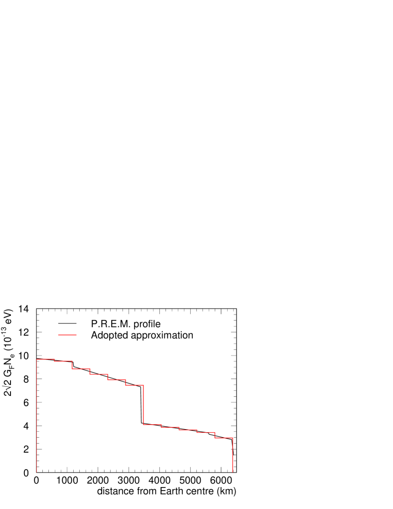
The explicit computation of transition probabilities has been addressed numerically. The Earth density profile of the Preliminary Reference Earth Model [10] has been approximated with eleven shells of constant density (see Fig. 1) and neutrino propagation has been computed from the (time ordered) product of evolution operators in matter of constant density:

$$\nu(L) = S(L)\nu(0)$$ (7)

$$= S_{n}(L_{n})S_{n-1}(L_{n-1})...~{}S_{1}(L_{1})\nu(0).$$

where $S_{i}(L_{i})$ describes the neutrino propagation along the path $L_{i}$ in the $i$-th shell and $n$ is the total number of shells crossed, which both depend on the neutrino angle.

Figure 2: In the upper and middle panels, the conversion probabilities for atmospheric neutrinos crossing the Earth are shown as a function of $L/E$ and $\cos\theta_{Nadir}$ for $\Delta m^{2}=+0.003$ eV² and $\sin^{2}(2\Theta_{13})=0.1$. The probability for $\overline{\nu}_{e}\to\overline{\nu}_{\mu}$ conversion is amplified by one order of magnitude to make it visible on the same scale as the other conversions. The lower panels shows the probability of observing muon neutrinos considering both $\nu_{\mu}\to\nu_{\mu}$ and $\nu_{e}\to\nu_{\mu}$ conversions and the neutrino fluxes.

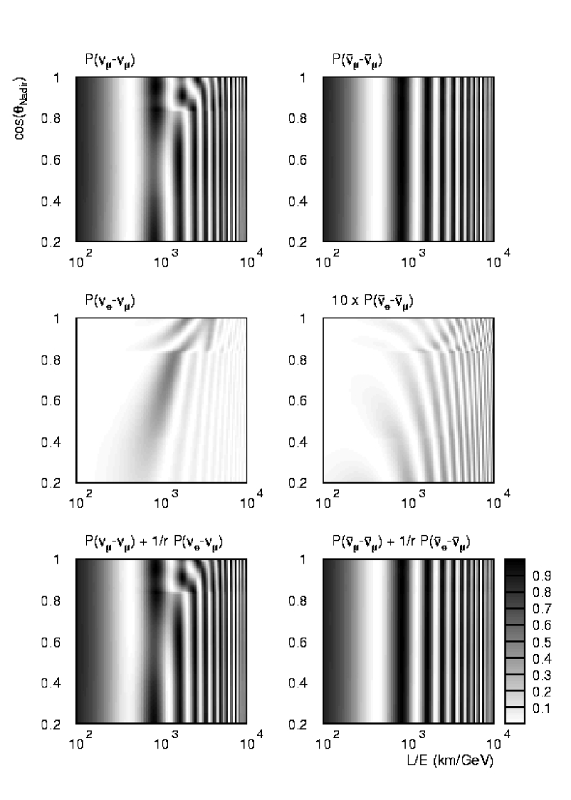
The $\nu_{\mu}\to\nu_{\mu}$ and $\nu_{e}\to\nu_{\mu}$ conversion probabilities as a function of $L/E$ and $\cos\theta_{Nadir}$ are shown in figure 2 for $\Delta m^{2}=+0.003$ eV² and $\sin^{2}2\Theta_{13}=0.1$. These values of oscillation parameters sit at the border of the 90% C.L. region excluded by CHOOZ. As a positive sign for $\Delta m^{2}$ was chosen, the $L/E$ pattern typical of vacuum oscillation is practically unaffected by matter effects for anti-neutrinos, while it is clearly modified for neutrinos. For neutrinos crossing the Earth’s core (i.e. $\cos\theta_{Nadir}>0.85$), sharp structures appear in the oscillation pattern. For lower values of $\cos\theta_{Nadir}$, the distortion with respect to the vacuum $L/E$ pattern for muon neutrinos is broader and most relevant around the first maximum, with a suppression of about 50%, and the second minimum of the conversion probability. Electron neutrino oscillations into muon neutrinos are correspondingly enabled in the same region of the $L/E$ and $\cos\theta_{Nadir}$ plane. The energy and angular regions of interest for these effects range from 4 GeV to 15 GeV and from $40^{o}$ to $60^{o}$, corresponding to a baseline of about 9000 km.

For smaller values of the mixing angle $\Theta_{13}$, the energy and angular positions of this distortion are almost independent of $\sin^{2}2\Theta_{13}$, but the distortion becomes sharper, in agreement with the expectations for neutrino propagation through a constant density medium (like the Earth’s mantle in first approximation).

The MONOLITH detector (see below) is optimized to reconstruct muon neutrinos and anti-neutrinos, the expected distribution of which is a combination of the conversion probabilities for $\nu_{\mu}\to\nu_{\mu}$ ($P_{\mu\mu}$) and $\nu_{e}\to\nu_{\mu}$ ($P_{e\mu}$) weighted by the corresponding neutrino fluxes. The probability of observing muon neutrinos is thus given by $P_{\mu\mu}+1/rP_{e\mu}$, where $r$ is the $\nu_{\mu}$ to $\nu_{e}$ flux ratio. Over the region where relevant matter effects occur, $r$ ranges between 2 and 3 and the disappearance of muon neutrinos through matter effects is only partly compensated by $\nu_{e}\to\nu_{\mu}$ transitions. This is shown in the lower panels of the figure for both neutrinos and anti-neutrinos: the flux suppression with respect to pure $\nu_{\mu}$–$\nu_{\tau}$ oscillations is still about 30% around the first maximum of the reappearance probability. The detailed simulation is addressed in the following.

3 Experiment simulation

The differential distribution of the atmospheric neutrino fluxes at Gran Sasso has been generated according to the predictions of the 1-D Bartol model [11]. Neutrino interactions have been calculated with GRV94 parton distributions [12] with explicit inclusion of the contribution of quasi-elastic scattering and of single pion production to the neutrino cross-sections [13].

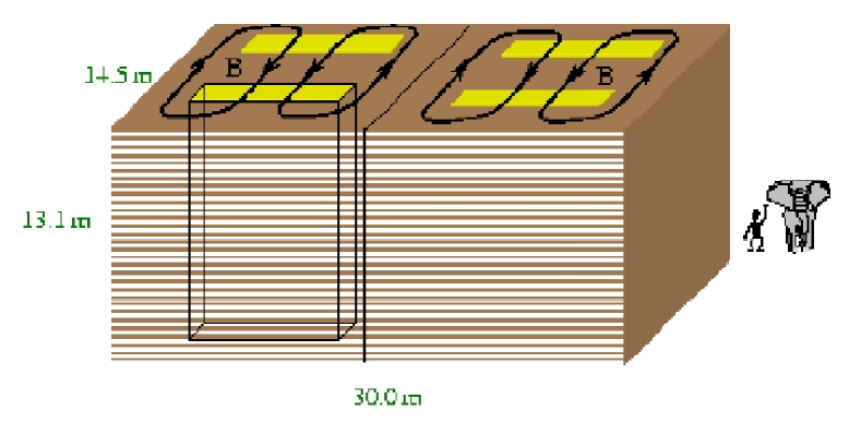
Events have been processed through the full simulation and reconstruction programs of the MONOLITH detector described in [5]. The proposed detector for MONOLITH is a massive tracking calorimeter with a coarse structure and intense magnetic field. The detector has a large modular structure (figure 3). One module consists in a stack of 120 horizontal 8 cm thick iron planes with a surface area of $14.5\times 15\ {\rm m^{2}}$, interleaved with 2 cm planes of sensitive elements. The total mass of the detector for two modules is about 34 kt. The magnetic field configuration is also shown in figure 3; iron plates are magnetized at a magnetic induction of $\approx 1.3$ T.

The active elements (Resistive plate chambers with glass electrodes [14]) provide two coordinates with a pitch of 3 cm and a time resolution of order 1 ns

Figure 3: Schematic view of the MONOLITH detector. The arrangement of the magnetic field is also shown.

After reconstruction, some minimal requests have been applied to select a pure sample of muon neutrino charged current interactions:

• a muon candidate firing at least 7 layers is required;

• the muon energy must exceed 1.5 GeV;

• the event is required to be either fully contained in a fiducial volume defined by requiring no hits in the first/last 4 layers and no hits in the first/last 10 strips in $X$ and $Y$, or to have a single outgoing track (muon) with a reconstructed range greater than 4 metres.

• the $L/E$ resolution of the event, determined from the angular and energy resolution and estimated from the event kinematic, is required to be better than 50% FWHM.

These selections guarantee a relatively high efficiency for an adequate resolution in the reconstruction of the neutrino energy and direction in the region of interest for matter effects. They result in an effective threshold around 3 GeV of neutrino energy and in a fairly constant efficiency between 50% and 55% from 5 GeV onwards. The neutrino angle is estimated from the muon direction with a resolution of about 15 degrees at 3 GeV and then improving with a $E_{\nu}^{-0.5}$ power law. The neutrino energy, estimated from the muon and hadron energy, shows a resolution of about 15-20% in the energy region where resonant effects are expected (4-15 GeV), smoothly broadening to 25% at very high energies, reflecting the worsening of the muon momentum resolution from track curvature. Charge assignment is correct in more than 95% of the cases, without additional requests on the track fit quality. The background due to internal and external sources is estimated to be negligible. More details on the MONOLITH performance can be found in [5].

Only internal events are selected and, in the energy region of interest for resonant effects, about 75% of these are fully contained in the detector. External events (up-going muons from neutrino interactions in the rock below the detector) are of little use in this study. Their average neutrino energy is much higher than the resonant energy and the resolution in the reconstruction of the neutrino energy is insufficient to resolve the typical resonance width.

4 Analysis and results

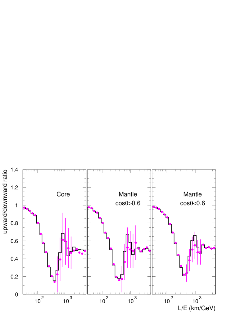
Although matter effects make the $L/E$ variable not sufficient for oscillation studies, an optimized analysis can be performed in the $L/E$ and $\cos\theta_{Nadir}$ plane. The energy of the resonance and the oscillation phase in vacuum scale both with $\Delta m^{2}$ and the main distortion to the vacuum oscillation pattern always occurs around the first maximum of the reappearance probability. As visible in figure 2, the $L/E$ pattern is only marginally modified over the first oscillation period by matter effects. This difference is even less evident when resolution and detector efficiency effects are considered (see Fig. 4). For $\Delta m^{2}=+0.003$ eV² and the largest values of $\sin^{2}2\Theta_{13}$ allowed by CHOOZ results, the distortion on the $L/E$ pattern (integrated over all neutrino baselines) is barely visible and located beyond the first minimum in the survival probability. As demonstarated in figure 5, this distortion is mainly due to neutrinos crossing the Earth’s mantle and in any case no distortions are predicted over the first half-period of oscillation. It follows that the measurement of the oscillation frequency from the position of the first minimum in the $L/E$ pattern is marginally affected by the presence of matter effects. The analysis of the $L/E$ pattern, assuming that no matter effects are present, will therefore precisely measure $\Delta m^{2}$ and tell where such effects have to be searched for in a two dimensional analysis (bin optimization).

Figure 4: Left: $L/E$ spectra for up-going (hatched histogram) and down-going muon neutrino (top) and muon anti-neutrino (bottom) events for three neutrino oscillations $\Delta m^{2}=+0.003$ eV², $\sin^{2}2\Theta_{23}=1.$ and $\sin^{2}2\Theta_{13}=0.1$. Right: Ratio of the up-going to down-going $L/E$ distributions. The curve represents the expectations for pure $\nu_{\mu}\to\nu_{\tau}$ oscillations. The experiment has been simulated with high statistics. Event rates and error bars are normalized to 6 y of MONOLITH exposure (200 kty).

Figure 5: $L/E$ spectra for up-going neutrinos crossing the Earth’s core (left) and mantle (middle and right) assuming $\Delta m^{2}=+0.003$ eV², $\sin^{2}2\Theta_{23}=1.$ and $\sin^{2}2\Theta_{13}=0.1$ (dots) compared to the expectations for pure $\nu_{\mu}\to\nu_{\tau}$ oscillations (histogram). The experiment has been simulated with high statistics. The error bars, shown only in the region where matter effects are sizeable, are normalized to 6 y of MONOLITH exposure (200 kty).

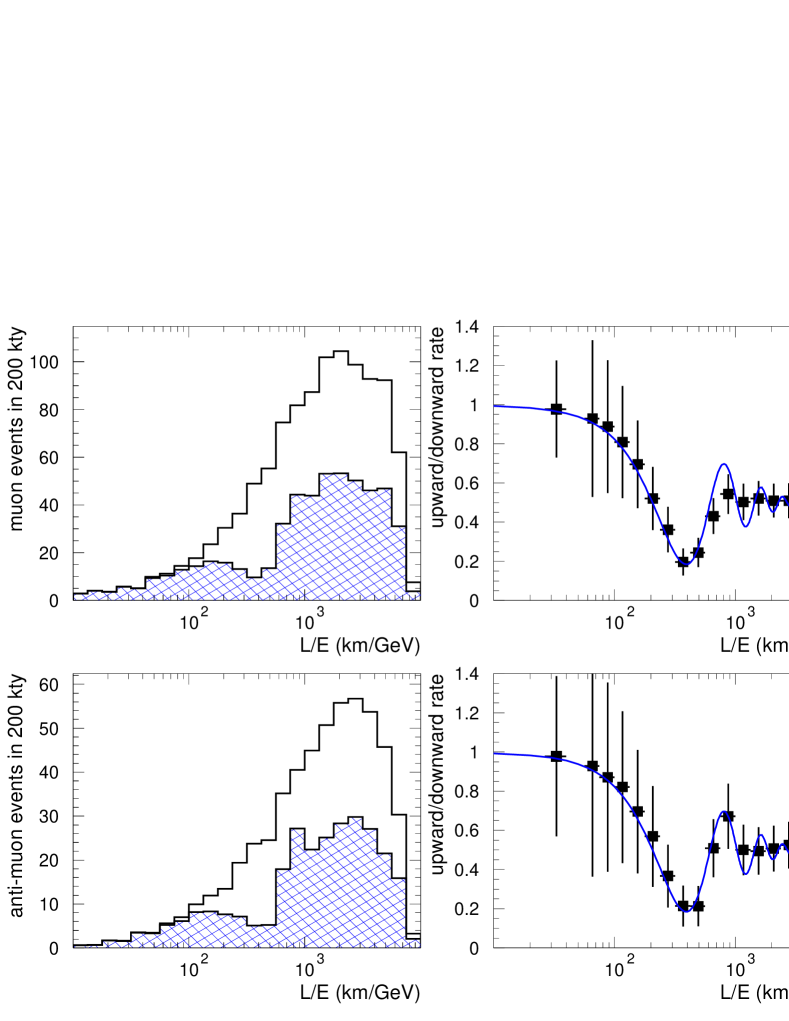
The analysis of simulated data has been based on a binned maximum likelihood fit. The expected $L/E$ distributions for neutrino and anti-neutrino events have been fitted to the reconstructed data from simulation in five $\cos\theta_{Nadir}$ bins of width 0.2. The binning in $L/E$ has been tuned according to the estimated value of $\Delta m^{2}$ from a preliminary fit of the $L/E$ distribution.

The expected number of events in each bin is a function of the oscillation parameters ($\Theta_{13},\Theta_{23},\Delta m^{2})$ and of the neutrino fluxes of all the flavours. In the real experiment, down-going neutrinos will constitute a reference sample of “unoscillated” neutrinos to check the muon neutrino and anti-neutrino rates. The rate of muon neutrinos originating from electron neutrino conversions will have to be predicted by flux calculations of electron neutrinos. These predictions will be constrained both by the measurement of the correlated rate of down-going muon neutrinos in the same detector and by the direct measurement of the electron neutrino to muon neutrino flux ratio in other experiments (Super-Kamiokande). A detailed study to quantify the related amount of systematic uncertainty has not been performed and an overall uncertainty of 10% in the predicted rates of neutrinos and anti-neutrinos has been assumed for a preliminary estimate of the experiment sensitivity.

The likelihood function has been defined as:

$$\ln{\cal L}=\ln\prod_{i,q}\left[\frac{e^{-A_{q}\mu_{i,q}}(A_{q}\mu_{i,q})^{U_{i,q}}}{U_{i,q}!}\right]-\sum_{q}\frac{1}{2}\frac{(A_{q}-1)^{2}}{\sigma_{A}^{2}}$$ (8)

where the subscripts $i$ and $q$ are referred to bins in the ($\cos\theta_{Nadir}$, $L/E$) plane and of muon charge respectively; $U_{i,q}$ and $A_{q}\mu_{i,q}$ are the observed and expected number of up-going neutrino events in the ${i,q}$-th bin and the last term in the likelihood accounts for flux, cross-section and selection efficiency uncertainties for neutrinos and anti-neutrinos separately.

Two different analyses have been performed to determine the sensitivity to the mixing parameter and to the sign of $\Delta m^{2}$.

4.1 Sensitivity to $\sin^{2}2\Theta_{13}$

In this analysis it has been assumed that the mixing in the (2,3) sector be maximal ($\sin^{2}2\Theta_{23}=1$). This corresponds to the best current estimate from Super-Kamiokande data. Individual experiments of high statistics have been generated for different values of $\sin^{2}2\Theta_{13}$ and $\Delta m^{2}$ and tested with a likelihood ratio analysis against the pure $\nu_{\mu}/\nu_{\tau}$ oscillation scenario (i.e. $\sin^{2}2\Theta_{13}=0$), assumed as null hypothesis. From this procedure, the values of the oscillation parameters that would give an experimental result incompatible with the null hypothesis have been determined. The likelihood ratio is defined by:

$$\lambda=\frac{{\cal L}(A_{q},\Delta m^{2},\sin^{2}2\Theta_{23},\sin^{2}2\Theta_{13}|\sin^{2}2\Theta_{13}=0)}{{\cal L}(A_{q},\Delta m^{2},\sin^{2}2\Theta_{23},\sin^{2}2\Theta_{13})},$$ (9)

representing the ratio of the maximum likelihood over the parameter space of the null hypothesis to the maximum likelihood over the entire parameter space. The test statistics $-2\ln\lambda$ asymptotically behaves as a $\chi^{2}(1)$ distribution, whence the iso-probability curves have been calculated. The expected and observed rates of events in the likelihood function of equation (8) have been normalized to represent experiments of finite statistics.

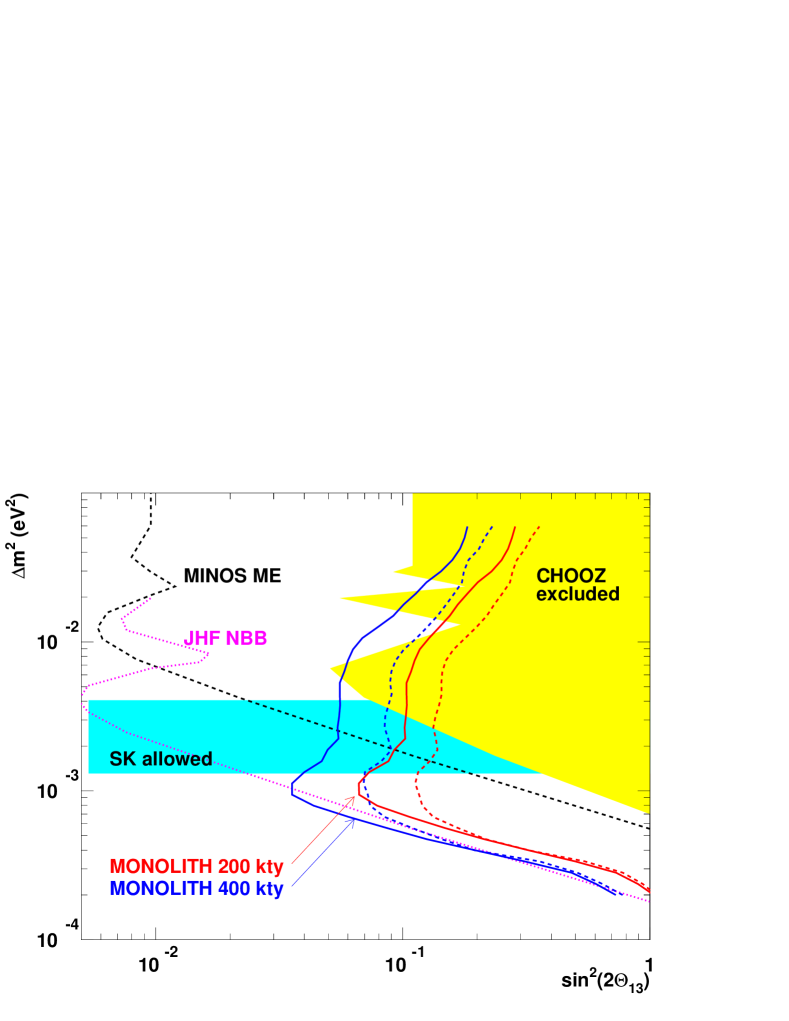
The expected sensitivities (exclusion regions at 90% C.L. if no effect is observed) after 200 kty of exposure (about 6 y for 34 kt) are shown in Fig. 6. Since the sign of $\Delta m^{2}$ is not known a͡ priori the curves for both positive (continuous line) and negative (dashed line) sign of $\Delta m^{2}$ are given. The expected exclusion region for positive sign of $\Delta m^{2}$ is about two times larger than for negative sign. This follows from the difference in neutrino and anti-neutrino cross sections, fluxes and selection efficiencies, which make the event rate of atmospheric neutrinos about two times larger than the rate of anti-neutrinos.

The sensitivity achievable in a long-term run (or with a larger detector), corresponding to an exposure of 400 kty, is also shown in the figure.

For comparison, the region excluded by CHOOZ results [7] and allowed by Super-Kamiokande data [15] are displayed. Also displayed are the expected sensitivities of neutrino oscillation programs with conventional neutrino beams in the short/medium term. The region covered by MONOLITH will be partly accessible to the MINOS experiment at NuMI [16] and fully accessible to the JHF beam to Super-Kamiokande [17]. The latter is expected to achieve this sensitivity around 2012 after 5 y of operation.

Figure 6: Exclusion regions at 90% C.L. if no matter effects are observed in MONOLITH after 200 kty (6 y) and 400 kty (12 y) of exposure. The curves for both positive (continuous line) and negative (dashed line) sign of $\Delta m^{2}$ are given. The regions excluded by CHOOZ results and allowed by Super-Kamiokande data are shown, together with the expected sensitivities of MINOS (Medium Energy option) and JHF projects (Low Energy option). The MINOS sensitivity is practically independent of the beam optics configuration in the region of $\Delta m^{2}$ allowed by Super-Kamiokande data. The JHF sensitivity can be better or worse than the one displayed by a factor of two depending on the beam optics.

4.2 Sensitivity to the sign of $\Delta m^{2}$

Figure 7: Upper panel: The continuous lines define the boundary of the regions of oscillation parameters in the three generation scenario over which the sign of $\Delta m^{2}$ can be determined at the 90% C.L. after MONOLITH exposures of 200 kty (6 y) and 400 kty (12 y), assuming that $\sin^{2}2\Theta_{13}$ be known with 30% accuracy. For comparison, the broken lines show the regions over which the sign of $\Delta m^{2}$ can be determined after 200 kty exposure assuming no prior knowledge on $\sin^{2}2\Theta_{13}$ regardless of the sign of $\Delta m^{2}$ (dotted) and for positive $\Delta m^{2}$ (dashed). The regions excluded by CHOOZ results at 90% C.L. and allowed by Super-Kamiokande at 90% C.L. data are also shown. Lower panel: Regions of oscillation parameters over which the sign of $\Delta m^{2}$ can be determined at the 3$\sigma$ level after MONOLITH exposures of 200 kty (6 y) and 400 kty (12 y), assuming that $\sin^{2}2\Theta_{13}$ be known with 30% accuracy.

Experiments at NuMI and JHF search directly for the sub-dominant $\nu_{\mu}\to\nu_{e}$ transition and have too short baselines to exploit matter effects. Thus, they cannot measure the sign of $\Delta m^{2}$.

With atmospheric neutrinos, if an effect is observed, the sign of $\Delta m^{2}$ can also be determined. Assuming no prior knowledge on $\sin^{2}2\Theta_{13}$, this happens at the 90% C.L. on the right-hand side of the dashed curves of figure 6, irrespectively of the sign of $\Delta m^{2}$, and on the right-hand side of the continuous curves, if $\Delta m^{2}$ is positive.

However, as discussed in the previous analysis, provided that the mixing $\sin^{2}2\Theta_{13}$ be large enough, there is a fair chance that it will be measured in the next generation of long base-lines experiments. In that case, this information can be used to constrain the maximum likelihood fit and and determine the sign of $\Delta m^{2}$ from the muon/anti-muon rate asymmetry.

The likelihood function of eq. (8) can be modified as:

$$\ln{\cal L}^{\prime}=\ln{\cal L}-\frac{1}{2}\frac{(\sin^{2}2\Theta_{13}-<\sin^{2}2\Theta_{13}>)^{2}}{\sigma_{13}^{2}}$$ (10)

In this analysis, $\sin^{2}2\Theta_{23}$ has been assumed to be maximal and $\sin^{2}2\Theta_{13}$ has been assumed to be known with an accuracy of 30%, representing the observation of a 3$\sigma$ effect at accelerator beams. Similarly to the analysis outlined in the previous section, individual experiments have been generated for different values of $\sin^{2}2\Theta_{13}$ and $\Delta m^{2}$. For each (absolute) value of $\Delta m^{2}$, the minimum value of $\sin^{2}2\Theta_{13}$ for which the best fit to data with the wrong sign of $\Delta m^{2}$ is incompatible with data has been determined.

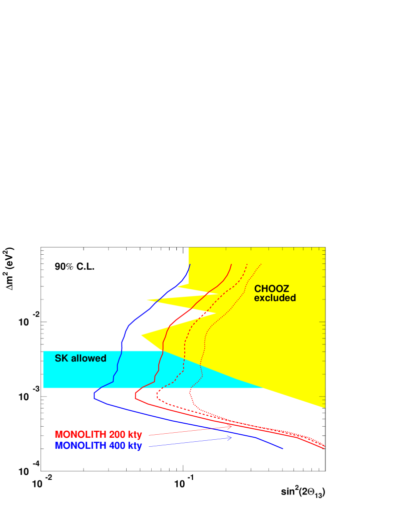
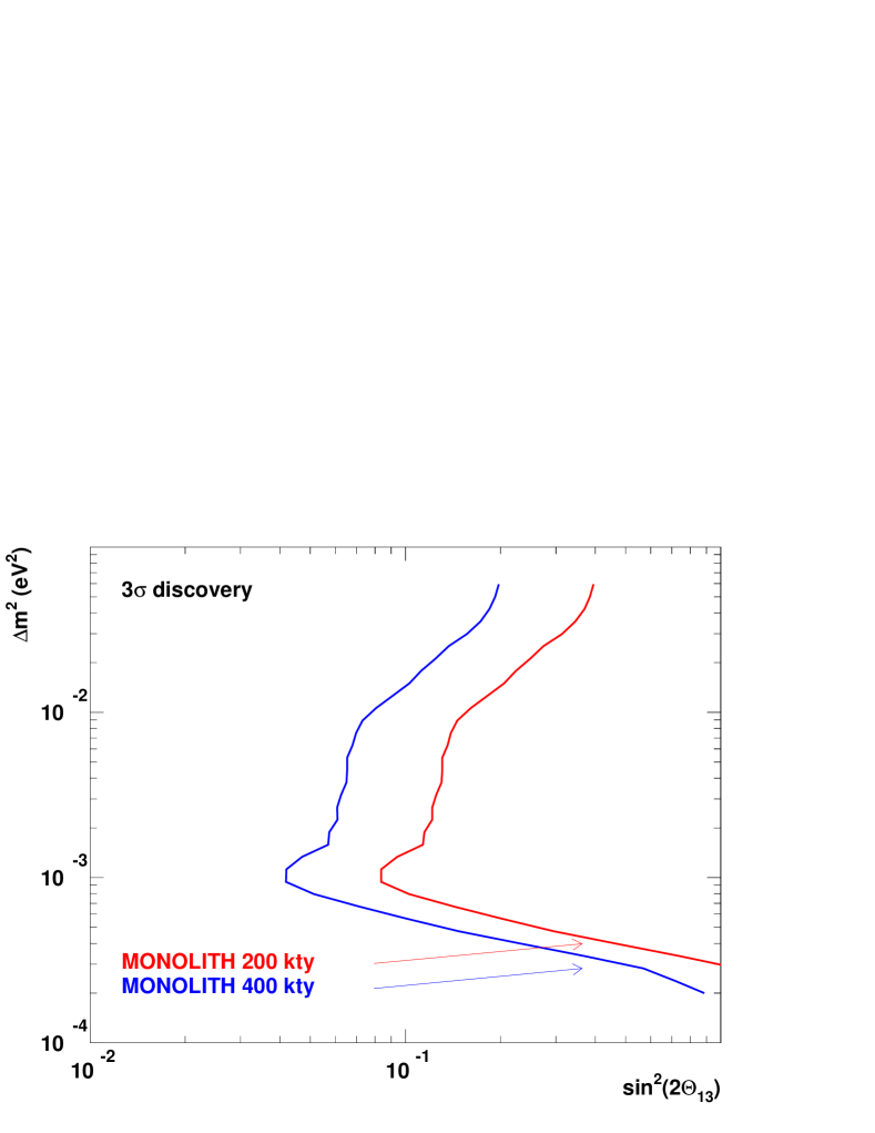
Figure 7 (upper panel) shows the expected region of oscillation parameters over which the sign of $\Delta m^{2}$ can be determined at the 90% C.L. after 200 kty of MONOLITH exposure (i.e. the wrong sign of $\Delta m^{2}$ is excluded at the 90% C.L.). The sensitivity achievable in a long-term run, corresponding to an exposure of 400 kty, is also shown. For comparison, the region excluded by CHOOZ [7] and the region allowed by Super-Kamiokande at 90% C.L. are displayed. On the same figure, the regions over which the the sign of $\Delta m^{2}$ can be determined after 200 kty of exposure without any prior knowledge of the (1,3) mixing are shown for comparison. The 3$\sigma$ discovery limit for the sign of $\Delta m^{2}$ is shown in the lower panel of the figure.

As expected, the additional constraint on the mixing parameter widen the sensitivity region and an exposure of 200 kty would be sufficient to evade the CHOOZ exclusion region. This is because in this case one has only to discriminate a positive from a negative asymmetry, while assuming no prior knowledge of the (1,3) mixing, an asymmetry of any sign should be discriminated from the no-asymmetry case.

5 Systematic uncertainties

Several sources of systematic uncertainties might affect the precision of this measurement.

The likelihood ratio method described by eq. (9) implies that no prior knowledge on the values of $\Delta m^{2}$ and $\sin^{2}2\Theta_{23}$ is assumed. These parameters can be measured in MONOLITH with an accuracy of about 5% with 200 kty exposure and reaching 1% for very large exposures. Since this would represent a substantial improvement with respect to the present knowledge, these parameters are not constrained in the fitting procedure.

The limited knowledge of the electron density profile in the Earth is also a source of systematic uncertainty. However, the sensitivity to matter effects with atmospheric neutrinos is dominated by the resonant behaviour of neutrinos crossing the bulk of the Earth’s mantle, whose density and chemical composition are known with sufficient precision. The matter density of the mantle is strongly constrained by the knowledge of the Earth’s mass and moment of inertia, combined with minimal information from seismic wave measurements of the density profile. The electron density is related to the matter density by the $Z/A$ ratio, which is very nearly 1/2 for all reasonable chemical compositions of the Earth’s mantle.

As discussed in section 4, the effects related to the limited knowledge of neutrinos and anti-neutrino fluxes and cross sections have been preliminary accounted for in this analysis by assigning an uncertainty of 10% to the predicted rates for neutrinos and anti-neutrinos separately. For an exact knowledge of these rates, the sensitivity regions shown in figure 6 would have to be extended by about 10%.

In a real experiment, the sample of down-going neutrino events can be exploited to constrain the neutrino and anti-neutrino event rate predictions. The precision of this procedure might be expected to scale with the square root of the exposure and will not be a fundamental limitation to the sensitivity to matter effects with atmospheric neutrinos. This is further discussed in the next section.

6 Very large exposures

The dependence of the experiment sensitivity on the exposure has been studied. The number of years of MONOLITH exposure has been increased up to represent a collected statistics of 2 Mty. Since selection and reconstruction efficiencies are the ones of MONOLITH, this simulation describes a detector (or array of detectors) of modular structure, with each single module comparable to MONOLITH in acceptance and performance.

Figure 8: Expected exclusion regions at 90% C.L. as a function of the exposure, if no matter effects are observed in MONOLITH. Data have been simulated with $\Delta m^{2}=+0.003$ eV². The continuous line shows the expected scaling behaviour, when the sensitivity is limited by statistical fluctuations (see text).

Figure 8 shows the expected sensitivity to $\sin^{2}2\Theta_{13}$ as a function of the exposure for $\Delta m^{2}=+0.003$. For negative sign of $\Delta m^{2}$ the sensitivity is about two times worse.

In this study, the systematic uncertainty related to the knowledge of the expected neutrino rates has been assumed to be 10% up to 400 kty and scaled with the square root of the exposure at the other points. Indeed, in a real experiment, down-going neutrino events will provide a reference sample of “unoscillated” neutrinos to check the expected muon neutrinos and anti-neutrinos rates with statistically increasing precision.

The sensitivity to matter effects would be expected to improve linearly with the exposure, if it were limited only by statistical fluctuations. In the region around the resonance, matter effects determine a $\nu/\overline{\nu}$ asymmetric variation in the event rate with respect to pure $\nu_{\mu}/\nu_{\tau}$ oscillations, that scales as the width of the resonance, i.e. $\sin 2\Theta_{13}=\sqrt{\sin^{2}2\Theta_{13}}$. This has to exceed the statistical fluctuations in the same region, which decrease as $1/\sqrt{T}$, where $T$ is the total exposure. Thus the expected exclusion limit on $\sin^{2}2\Theta_{13}$ should scale as $1/T$.

As shown in the figure, this scaling law holds up to an exposure of around 1 Mty, corresponding to a sensitivity around 0.02 on the mixing parameter. Beyond that limit, the width of the resonance in the Earth mantle becomes comparable to the energy resolution of the experiment and the resonance cannot be fully resolved. An improvement in the energy resolution would thus be necessary to further push the sensitivity to matter effects for $\sin^{2}2\Theta_{13}$ below 0.01.

Following the discussion given in [6], for values of the mixing parameter this low, the observation of the resonance should also be inhibited by other reasons. A sizeable distortion of the oscillation pattern can be observed only when an overlap between the resonance in the effective mixing and the oscillation factor occurs. According to this argument, in a medium of constant density the observability of the resonance requires a minimum baseline, whose length scales as $1/\tan 2\Theta_{13}$. For mixings as small as 0.01, this baseline exceeds the Earth’s diameter.

7 Conclusions

A study of the sensitivity of a massive magnetized detector for atmospheric neutrinos (MONOLITH) to matter effects in the framework of a three flavour scenario with one mass scale dominance for atmospheric neutrinos has been reported.

A sub-dominant component of $\nu_{e}$ mixing could give rise to resonant $\nu_{\mu}\leftrightarrow\nu_{e}$ transitions in matter, which occur either for neutrinos or for anti-neutrinos only, depending on the sign of $\Delta m^{2}$. This can be exploited in a magnetized detector to determine the sign of $\Delta m^{2}$ and therefore the neutrino mass hierarchy. The size of this effect would also measure the mixing of electron neutrinos.

About 200 kty of MONOLITH exposure will be sufficient to explore regions not yet ruled out by the bound on $\nu_{e}\to\nu_{\mu}$ oscillations derived by CHOOZ results [7]. These regions will be partly accessible to MINOS and JHF [16, 17], which, however, can not measure the sign of $\Delta m^{2}$.

The sensitivity achievable in a high statistics run has also been discussed. The ultimate sensitivity which can be achieved with exposures of 1-2 Mty would be $\sin^{2}2\Theta_{13}\sim 0.01$. In order to go below this limit, the energy resolution would have to be improved. For values of $\sin^{2}2\Theta_{13}$ this low, the observability of the resonance is also compromised by the fact that the maximum of the effective mixing is somehow compensated by a minimum in the oscillation factor over the Earth’s dimension.

References

- [1] V. Barger, D. Marfatia and K. Whisnant, preprint hep-ph/0108090 (2001)
- [2] C. Albright et al., preprint hep-ex/0008064 (2000).
- [3] Y. Fukuda et al. (Super-Kamiokande Coll.) Phys. Rev. Lett. 85 (2000) 3999.
- [4] H. Habig (for the Super-Kamiokande Coll.), preprint hep-ex/0106025 (2001).
- [5] N.Y. Agafonova et al., The MONOLITH Proposal, LNGS P26/2000, CERN/SPSC 2000-031, August 2000 (available at http://castore.mib.infn.it/∼monolith/proposal/).
- [6] M.C. Bañuls, G. Barenboim and J. Bernabéu, Phys. Lett. B 513 (2001) 391.
-
[7]
M. Apollonio et al. (CHOOZ Collaboration),
Phys. Lett. B 420 (1998) 397;
M. Apollonio et al. (CHOOZ Collaboration), Phys. Lett. B 466 (1999) 415. -
[8]
R. Barbieri et al., JHEP 12 (1998) 017
V. Barger, T.J. Weiler, K. Whisnant, Phys. Lett. B 440 (1998) 1;
G.L. Fogli, E. Lisi, A. Marrone, L. Scioscia, Phys.Rev. D 59 (1999) 033001. - [9] A. Aguilar et al. (LNSD Collaboration), hep-ex/0104049 and references therein.
- [10] A.M. Dziewonski and D.L. Anderson, Phys. Earth Planet. Inter., 25 (1981) 297
- [11] V. Agrawal, T.K. Gaisser, P. Lipari and T. Stanev, Phys. Rev. D 53 (1996) 1314.
- [12] M. Gluck, E. Reya and A. Vogt, Z. Phys. C 67 (1995) 433.
- [13] P. Lipari, M. Lusignoli and F. Sartogo, Phys. Rev. Lett. 74 (1995) 4384.
- [14] G. Bencivenni et al., Nucl. Instrum. Meth. A 461 (2001) 319.
- [15] T. Toshito (for the Super-Kamiokande Coll.), preprint hep-ex/0105023 (2001).
- [16] A. Para, preprint hep-ph/0005012 (2000).
[17]
Y. Itow et al., preprint hep-ex/0106019 (2001);
T. Nagae, Nucl. Phys. A 639 (1998) 551.