Impact of two mass-scale oscillations on the analysis of atmospheric and reactor neutrino data

Abstract

We study the stability of the results of 3-$\nu$ oscillation analysis of atmospheric and reactor neutrino data under departures of the one–dominant mass scale approximation. In order to do so we perform the analysis of atmospheric and reactor neutrino data in terms of three–neutrino oscillations where the effect of both mass differences is explicitly considered. We study the allowed parameter space resulting from this analysis as a function of the mass splitting hierarchy parameter $\alpha=\Delta m^{2}/\Delta M^{2}$ which parametrizes the departure from the one–dominant mass scale approximation. We consider schemes with both direct and inverted mass ordering. Our results show that in the analysis of atmospheric data the derived range of the largest mass splitting, $\Delta M^{2}$, is stable while the allowed ranges of mixing angles $\sin^{2}\theta_{23}$ and $\sin^{2}\theta_{13}$ are wider than those obtained in the one–dominant mass scale approximation. Inclusion of the CHOOZ reactor data in the analysis results into the reduction of the parameter space in particular for the mixing angles. As a consequence the final allowed ranges of parameters from the combined analysis are only slightly broader than when obtained in the one–dominant mass scale approximation.

1 Introduction

Super–Kamiokande (SK) high statistics data skatmlast indicate that the observed deficit in the $\mu$-like atmospheric events is due to the neutrinos arriving in the detector at large zenith angles, strongly suggestive of the $\nu_{\mu}$ oscillation hypothesis. Similarly, the latest SNO results sno ; snonc in combination with the Super–Kamiokande data on the zenith angle dependence and recoil energy spectrum of solar neutrinos sksollast and the Homestake chlorine , SAGE sage , and GALLEX+GNO gallex ; gno experiments, have put on a firm observational basis the long–standing problem of solar neutrinos snp , strongly indicating the need for $\nu_{e}$ conversions.

Altogether, the solar and atmospheric neutrino anomalies constitute the only solid present–day evidence for physics beyond the Standard Model review . It is clear that the minimum joint description of both anomalies requires neutrino conversions among all three known neutrinos. In the simplest case of oscillations the latter are determined by the structure of the lepton mixing matrix MNS , which, in addition to the Dirac-type phase analogous to that of the quark sector, contains two physical phases associated to the Majorana character of neutrinos, which however are not relevant for neutrino oscillation majophases and will be set to zero in what follows. In this case the mixing matrix $U$ can be conveniently chosen in the form PDG

$$\left(\begin{array}[]{ccc}c_{13}c_{12}&s_{12}c_{13}&s_{13}\,{e}^{-i\delta}\\ -s_{12}c_{23}-s_{23}s_{13}c_{12}\,{e}^{i\delta}&c_{23}c_{12}-s_{23}s_{13}s_{12}\,{e}^{i\delta}&s_{23}c_{13}\\ s_{23}s_{12}-s_{13}c_{23}c_{12}\,{e}^{i\delta}&-s_{23}c_{12}-s_{13}s_{12}c_{23}\,{e}^{i\delta}&c_{23}c_{13}\end{array}\right)\,,$$ (1)

where $c_{ij}\equiv\cos\theta_{ij}$ and $s_{ij}\equiv\sin\theta_{ij}$. Thus the parameter set relevant for the joint study of solar and atmospheric conversions becomes six-dimensional: two mass differences, three mixing angles and one CP phase.

Results from the analysis of solar and atmospheric data in the framework of two-neutrino oscillation 2solour ; 2solother ; 2atm ; 3atmfogli imply that the required mass differences satisfy

$$\Delta m^{2}_{\odot}\ll\Delta m^{2}_{\rm atm}.$$ (2)

For sufficiently small $\Delta m^{2}_{\odot}$ the three-neutrino oscillation analysis of the atmospheric neutrino data can be performed in the one mass scale dominance approximation neglecting the effect of $\Delta m^{2}_{\odot}$. In this approximation it follows that the atmospheric data analysis restricts three of the oscillation parameters, namely, $\Delta m^{2}_{31}=\Delta m^{2}_{32}$, $\theta_{23}$ and $\theta_{13}$. This is the approximation used in Ref. 3atmfogli ; 3ours ; 3atm . Conversely for the solar neutrino analysis the effect of oscillations with $\Delta m^{2}_{\rm atm}$ can be taken to be averaged and solar data constrains $\Delta m^{2}_{21},\theta_{12}$ and $\theta_{13}$ 3ours ; 3sol . In this approximation the reactor neutrino data from CHOOZ provides information on the atmospheric mass difference and the mixing angle $\theta_{13}$, and the CP phase $\delta$ becomes unobservable.

However the assumption of one mass scale dominance may not be a good approximation neither for reactor nor for atmospheric data, in particular for $\Delta m^{2}_{\odot}$ in its upper allowed values. Effects of the departure of the one mass scale dominance approximation in the analysis of the CHOOZ reactor data CHOOZ has been included in Ref. 3ours ; choozpetcov ; irina . For atmospheric neutrinos in Refs. strumia ; 3atmfogli ; antonio it was shown that oscillations with two mass scales of the order of $10^{-3}$ could give a good description of the existing data for some specific values of the parameters. Some analytical approximate expressions for the effects of keeping both mass scales in the description of atmospheric neutrinos are presented in Refs. smirnov1 ; smirnov2 ; nohierothers . Furthermore Refs. smirnov1 ; smirnov2 describe how the presence of the second mass scale can lead to an increase in the number of sub-GeV electron events which seems to improve the description of the observed distribution.

To further explore this possibility and to verify the consistency of the one–dominant mass scale approximation we present in this work the result of the analysis of the atmospheric and reactor neutrino data in terms of three-neutrino oscillations where the effect of both mass differences is explicitly considered and we compare our results with those obtained under the assumption of one-dominant scale. Our aim is to study how/whether the allowed parameter space is modified as a function of the ratio between the two mass scales. Our study allow us to establish the stability of the derived ranges of parameters for the large mass scale and mixings $\theta_{23}$ and $\theta_{13}$ independently of the exact value of the solar small scale and mixing $\theta_{12}$ for which we only chose it to be within the favoured LMA region. Our results show that the allowed ranges of parameters from the combined atmospheric plus reactor data analysis are only slightly broader than when obtained in the one–dominant mass scale approximation. Thus our main conclusion is that the approximation is self-consistent. To establish the relevance of each data sample on this conclusion we also present the partial results of the analysis including only the atmospheric data or the reactor data.

The outline of this paper is as follows. In Sec. 2 we describe our notation for the parameters relevant for atmospheric and reactor neutrino oscillations with two mass scales and discuss the results for the relevant probabilities. In Sec. 3 and 4 we show our results for the analysis of atmospheric neutrino and reactor data respectively. For atmospheric neutrinos we include in our analysis all the contained events from the latest 1489 SK data set skatmlast , as well as the upward-going neutrino-induced muon fluxes from both SK and the MACRO detector MACRO . The results for the combined analysis are described in Sec. 5. Finally in Sec. 6 we summarize the work and present our conclusions.

2 Three Neutrino Oscillations with Two Mass Scales

In this section we review the theoretical calculation of the conversion probabilities for atmospheric and reactor neutrinos in the framework of three–neutrino mixing, in order to set our notation and to clarify the approximations used in the evaluation of such probabilities.

In general, the determination of the oscillation probabilities for atmospheric neutrinos require the solution of the Schrödinger evolution equation of the neutrino system in the Earth–matter background. For a three-flavour scenario, this equation reads

$$i\frac{d\vec{\nu}}{dt}={\bf H}\,\vec{\nu},\qquad{\bf H}={\bf U}\cdot{\bf H}_{0}^{d}\cdot{\bf U}^{\dagger}+{\bf V}\,,$$ (3)

where ${\bf U}$ is the unitary matrix connecting the flavour basis and the mass basis in vacuum and which can be parametrized as in Eq. (1). On the other hand ${\bf H}_{0}^{d}$ and V are given as

$${\bf H}_{0}^{d}=\frac{1}{2E_{\nu}}{\bf diag}\left(0,\Delta m^{2}_{21},\Delta m^{2}_{31}\right),$$ (4)

$${\bf V}={\bf diag}\left(\pm\sqrt{2}G_{F}N_{e},0,0\right),$$ (5)

where $\vec{\nu}\equiv\left(\nu_{e},\nu_{\mu},\nu_{\tau}\right)$. We have denoted by ${\bf H}_{0}^{d}$ the vacuum Hamiltonian, while ${\bf V}$ describes charged-current forward interactions in matter MSW . In Eq. (5), the sign $+$ ($-$) refers to neutrinos (antineutrinos), $G_{F}$ is the Fermi coupling constant and $N_{e}$ is electron number density in the Earth (note also that for antineutrinos, the phase $\delta$ has to be replaced with $-\delta$).

Figure 1: Our convention for the mass splitting and ordering.

The angles $\theta_{ij}$ can be taken without any loss of generality to lie in the first quadrant $\theta_{ij}\in[0,\pi/2]$. Concerning the CP violating phase $\delta$ we chose the convention $0\leq\delta\leq\pi$ and two choices of mass ordering (See Fig. 1) one with $m_{1}\leq m_{2}\leq m_{3}$ which we will denote as Normal and other with $m_{3}\leq m_{1}\leq m_{2}$ which we will denote as Inverted (for a recent discussion on other conventions see, for instance zralek ). We define as $\Delta M^{2}>0$ the large mass splitting in the problem and $\Delta m^{2}>0$ the small one. In this case we can have the two mass ordering:

Normal: $$\Delta M^{2}=\Delta m^{2}_{31}=m_{3}^{2}-m_{1}^{2}$$ (6)

$$\Delta m^{2}=\Delta m^{2}_{21}=m_{2}^{2}-m_{1}^{2}\;\,$$

Inverted: $$\Delta M^{2}=-\Delta m^{2}_{32}=m_{2}^{2}-m_{3}^{2}$$ (7)

$$\Delta m^{2}=\Delta m^{2}_{21}=m_{2}^{2}-m_{1}^{2}\,.$$

We define the mass splitting hierarchy parameter

$$\alpha=\frac{\Delta m^{2}}{\Delta M^{2}}\,,$$ (8)

which parametrizes the departure from the one–dominant mass scale approximation in the analysis of atmospheric and reactor neutrinos.

In this convention, for both Normal or Inverted schemes, the mixing angles in Eq. (1) are such that in the one mass dominance approximation in which $\Delta M^{2}$ ($\Delta m^{2}$) determines the oscillation length of atmospheric (solar) neutrinos, $\theta_{23}$ is the mixing angle relevant for atmospheric oscillations while $\theta_{12}$ is the relevant one for solar oscillations, and $\theta_{13}$ is mostly constrained by reactor data. In the likely situation in which the solar solution is LMA, $\theta_{12}$ is mainly restricted to lie in the first octant.

We will restrict ourselves to the CP conserving scenario. CP conservation implies that the lepton phase $\delta$ is either zero or $\pi$ Schechter:1981hw . As we will see, for non-vanishing $\alpha$ and $\theta_{13}$ the analysis of atmospheric neutrinos is not exactly the same for these two possible CP conserving values of $\delta$ and we characterize these two possibilities in terms of $\cos\delta=\pm 1$.

For $\alpha=\theta_{13}=0$, atmospheric neutrinos involve only $\nu_{\mu}\to\nu_{\tau}$ conversions, and in this case there are no matter effects, so that the solution of Eq. (3) is straightforward and the conversion probability takes the well-known vacuum form

$$P_{\mu\mu}=1-\sin^{2}\left(2\theta_{23}\right)\sin^{2}\left(\frac{\Delta M^{2}L}{4E_{\nu}}\right),$$ (9)

where $L$ is the path-length traveled by neutrinos of energy $E_{\nu}$.

On the other hand, in the general case of three-neutrino scenario with $\theta_{13}\neq 0$ or $\alpha\neq 0$ the presence of the matter potentials become relevant and it requires a numerical solution of the evolution equations in order to obtain the oscillation probabilities for atmospheric neutrinos $P_{\alpha\beta}$, which are different for neutrinos and anti-neutrinos because of the reversal of sign in Eq. (5). In our calculations, we use for the matter density profile of the Earth the approximate analytic parametrization given in Ref. lisi of the PREM model of the Earth PREM .

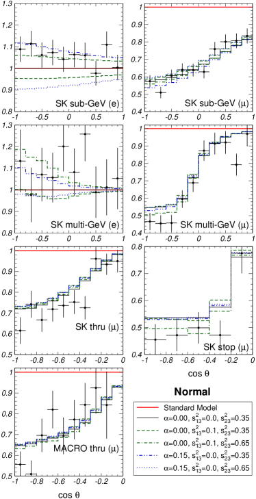
Figure 2: Zenith-angle distributions (normalized to the no-oscillation prediction) for the Super–Kamiokande $e$–like and $\mu$–like contained events, for the Super–Kamiokande stopping and through-going muon events and for Macro upgoing muons. The various dashed lines are the expected distributions for the Normal mass ordering with $\Delta M^{2}=3\times 10^{-3}$ eV², $\tan^{2}\theta_{12}=0.45$ and several values of $\sin^{2}\theta_{13}$ and $\sin^{2}\theta_{23}$ as given in the figure.

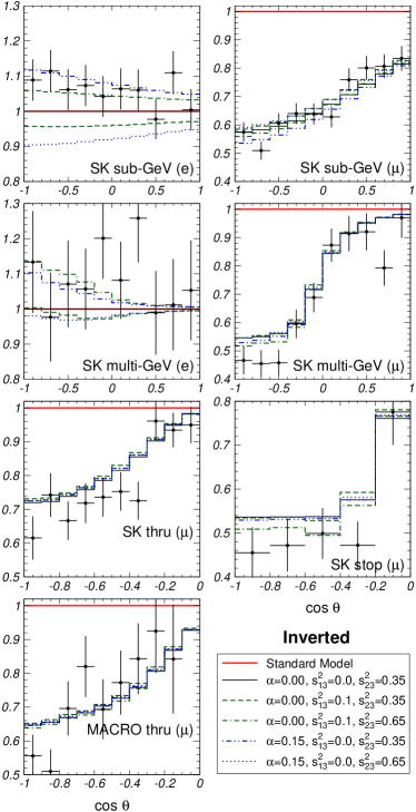
Figure 3: Same as Fig. 2 but for Inverted mass ordering.

In Figs. 2 and 3 we plot the angular distribution of atmospheric $\nu_{e}$ and $\nu_{\mu}$ for non-vanishing values of $\alpha$ or $\theta_{13}$ obtained from our numerical calculations. As seen in these figures the main effect of a small but non-vanishing $\alpha$ is mostly observable for sub-GeV electrons, although some effect is also visible for multi-GeV electrons and sub-GeV muons, and it can result either in an increase or in a decrease of the expected number of events with respect to the $\alpha=0$ prediction depending on whether $\theta_{23}$ is in the first or second octant. This behaviour can be understood in terms of the approximate analytical expressions. For instance for $\theta_{13}=0$ we find (in agreement with the results in Ref. smirnov1 )

$$\frac{N_{e}}{N_{e0}}-1 = \overline{P}_{e2}\bar{r}(c_{23}^{2}-\frac{1}{\bar{r}})$$ (10)

$$\frac{N_{\mu}-N_{\mu}(\alpha=0)}{N_{\mu 0}} = -\overline{P}_{e2}c_{23}^{2}(c_{23}^{2}-\frac{1}{\bar{r}})$$ (11)

where $N_{e0}$ and $N_{\mu 0}$ are the expected number of electron and muon-like events in the absence of oscillations in the relevant energy and angular bin and $\bar{r}=N_{\mu 0}/N_{e0}$. For instance, for sub-GeV events $\bar{r}\sim 2$. Here $N_{\mu}(\alpha=0)$ is the expected number of muon-like events for $\alpha=0$ and $\overline{P}_{e2}$ is the dominant $\alpha$-dependent term in the probabilities, averaged over energy and zenith angle. For neutrinos we have:

$$P_{e2} = \sin^{2}2\theta_{12,m}\sin^{2}\left(\frac{\Delta m^{2}\,L}{4E_{\nu}}\frac{\sin 2\theta_{12}}{\sin 2\theta_{12,m}}\right)\,,$$ (12)

$$\sin 2\theta_{12,m} = \frac{\sin 2\theta_{12}}{\sqrt{(\cos 2\theta_{12}-2E_{\nu}V_{e}/\Delta m^{2})^{2}+(\sin 2\theta_{12})^{2}}}\,,$$

which for $\Delta m^{2}\ll 2E_{\nu}V_{e}$ reduces to:

$$P_{e2}=\alpha^{2}\sin^{2}2\theta_{12}\left(\frac{\Delta M^{2}}{2EV_{e}}\right)^{2}\sin^{2}\frac{V_{e}L}{2}\,.$$ (13)

According to Eqs. (10) and (11) the sign of the shift in the number of predicted events with respect to the results in the one mass scale dominance approximation is opposite for electron and muon-like events and it depends on the factor $c_{23}^{2}-\frac{1}{\bar{r}}\sim c_{23}^{2}-0.5$. So for $\theta_{23}$ in the first octant, $c_{23}^{2}>0.5$, there is an increase (decrease) in the number of electron (muon) events as compared to the $\alpha=0$ case. For $\theta_{23}$ in the second octant the opposite holds. We also see that the net shift is larger for electron events than for muon events by a factor $c_{23}^{2}/\bar{r}$. Notice that, despite Eq. (13) looks order $\alpha^{2}$, its numerical value for sub-GeV electrons is large due to the factor $\Delta M^{2}/(2EV_{e})$ as can be seen from the figures. At higher energies, for up-going muons the effect is negligible.

For the sake of comparison we also show in the figures the behaviour with non-vanishing value of $\theta_{13}$ in the one mass scale dominance approximation. As seen in the figure the effect is most important for the electron events and can be understood as follows. For the case of constant matter density the expected flux of $\nu_{e}$ events in the one mass scale dominance approximation we find

$$\frac{N_{e}}{N_{e0}}-1=\overline{P}_{e\mu}\bar{r}(s_{23}^{2}-\frac{1}{\bar{r}})$$ (14)

where

$$P_{e\mu} = 4s^{2}_{13,m}c^{2}_{13,m}\sin^{2}\left(\frac{\Delta M^{2}\,L}{4E_{\nu}}\frac{\sin 2\theta_{13}}{\sin 2\theta_{13,m}}\right)\,,$$ (15)

$$\sin 2\theta_{13,m} = \frac{\sin 2\theta_{13}}{\sqrt{(\cos 2\theta_{13}\mp 2E_{\nu}V_{e}/\Delta M^{2})^{2}+(\sin 2\theta_{13})^{2}}}$$

and the $-$ (+) sign applies for the Normal (Inverted) case (similar expression is presented, for instance, in the last article in Ref. 2atm and in Ref. atmpetcov ). So for $\theta_{23}$ in the first octant ($s_{23}^{2}<0.5$) there is a decrease in the number of electron events as compared to the $\theta_{13}$ case. For sub-GeV events, the matter term in Eq. (15) can be neglected and the effect of a non-vanishing $\theta_{13}$ is the same for Normal and Inverted ordering. For multi-GeV and upgoing muon events matter effects start playing a role and the effect becomes slightly larger for the Normal case where the matter enhancement is in the neutrino channel.

The situation becomes more involved when both $\alpha$ and $\theta_{13}$ are different from zero. For instance, in lowest order in $\alpha$ $s_{13}$ the expected number of sub-GeV $\nu_{e}$ events is (after averaging the $\Delta M^{2}L/E$ oscillations)

$$\frac{N_{e}}{N_{e0}}-1 = \overline{P}_{e2}\,\bar{r}\,(c_{23}^{2}-\frac{1}{\bar{r}})+\overline{P}_{e\mu}\,\bar{r}\,(s_{23}^{2}-\frac{1}{\bar{r}})$$

$$+ \frac{\bar{r}}{2}\cos\delta\sin 2\theta_{13}\sin 2\theta_{23}\sin 2\overline{\theta}_{12,m}\cos 2\overline{\theta}_{12,m}$$

$$\overline{\sin^{2}\left(\frac{\Delta m^{2}\,L}{4E_{\nu}}\frac{\sin 2\theta_{12}}{\sin 2\theta_{12,m}}\right)}$$

(this expression is in agreement with the results in Ref. smirnov2 ). From this equation we see that the interference term (the third term in the right hand side) can have either sign depending on $\cos\delta$. It also changes sign depending on whether the $\Delta m^{2}$ oscillations are above ($\Delta m^{2}\cos 2\theta_{12}>2E_{\nu}V_{e}$) of below ($\Delta m^{2}\cos 2\theta_{12}<2E_{\nu}V_{e}$) the resonance. For very small $\alpha$ ($\Delta m^{2}\ll 2E_{\nu}V_{e})$ the interference term is proportional to $\alpha$ and it also changes sign for neutrinos and antineutrinos. In summary the effect of non-vanishing $\theta_{13}$ and $\alpha$ in the expected number and distribution of atmospheric neutrino events can have opposite signs and this can lead to a partial cancellation between both contributions. This results into a loss of sensitivity of the analysis to both parameters.

To analyze the CHOOZ constraints we need to evaluate the survival probability for ${\bar{\nu}}_{e}$ of average energy $E\sim$ few MeV at a distance of $L\sim 1$ Km. For these values of energy and distance, one can safely neglect Earth matter effects. The survival probability takes the analytical form:

$$P_{ee}^{\rm CHOOZ} = 1-\cos^{4}\theta_{13}\sin^{2}2\theta_{12}\sin^{2}\left(\frac{\Delta m^{2}_{21}L}{4E_{\nu}}\right)$$

$$-\sin^{2}2\theta_{13}\left[\cos^{2}\theta_{12}\sin^{2}\left(\frac{\Delta m^{2}_{31}L}{4E_{\nu}}\right)\right.$$

$$\left.+\sin^{2}\theta_{12}\sin^{2}\left(\frac{\Delta m^{2}_{32}L}{4E_{\nu}}\right)\right]$$

$$\simeq 1-\sin^{2}2\theta_{13}\sin^{2}\left(\frac{\Delta M^{2}L}{4E_{\nu}}\right),$$

where the second equality holds under the approximation $\Delta m^{2}\ll E_{\nu}/L$ which can only be safely made for $\Delta m^{2}\leq 3\times 10^{-4}~{}$eV². Eq. (2) is valid for both Normal and Inverted ordering with the identifications in Eq.(6) and Eq.(7) respectively. It results that the probability for Normal and Inverted schemes is the same with the exchange $\sin^{2}\theta_{12}\leftrightarrow\cos^{2}\theta_{12}$. Thus in general the analysis of the CHOOZ reactor data involves four oscillation parameters: $\Delta M^{2}$, $\theta_{13}$, $\Delta m^{2}$, and $\theta_{12}$. From Eq. (2) we see that for a given value of $\theta_{12}$ and $\Delta M^{2}$ the effect of a non-vanishing value of either $\theta_{13}$ or $\Delta m^{2}$ is the decrease of the survival probability.

3 Atmospheric Neutrino Analysis

In our statistical analysis of the atmospheric neutrino events we use all the samples of SK data: $e$-like and $\mu$-like samples of sub- and multi-GeV skatmlast data, each given as a 10-bin zenith-angle distribution , and upgoing muon data including the stopping (5 bins in zenith angle) and through-going (10 angular bins) muon fluxes. We have also included the latest MACRO MACRO upgoing muon samples, with 10 angular bins. So we have a total of 65 independent inputs.

For details on the statistical analysis applied to the different observables, we refer to the first reference in Refs. 2atm and 3ours . As discussed in the previous section, the analysis of the atmospheric neutrino data for three neutrino oscillations with two mass scales involves six parameters: two mass differences, three mixing angles and one CP phase. Our aim is to study the modification on the resulting allowed ranges of the parameters $\Delta M^{2}$, $\sin^{2}\theta_{23}$ and $\sin^{2}\theta_{13}$ due to the deviations from the one–dominant mass scale approximation, i.e. for $\Delta m^{2}\neq 0$ (or equivalently for non-vanishing values of mass splitting hierarchy parameter $\alpha$). In what follows, for the sake of simplicity, we will restrict ourselves to the CP conserving scenario but we will distinguish the two possible CP conserving values of $\delta$ and we characterize these two possibilities in terms of $\cos\delta=\pm 1$. We will show the results for Normal and Inverted schemes. Furthermore in most of our study we will keep the mixing angle $\theta_{12}$ to be within the LMA range favoured in the global analysis of solar neutrino data by choosing a characteristic value $\tan^{2}\theta_{12}=0.45$ 2solour ; 2solother . We have repeated our analysis for different values of $\theta_{12}$ and we have found that the maximum effect due to the variation of $\theta_{12}$ is a shift on $\Delta\chi^{2}\sim 1$ and it is therefore unobservable. Furthermore we have verified that the atmospheric data analysis does not provide enough precision to test the possibility of non-vanishing CP violation.

We first present the results of the allowed parameters for the global combination of atmospheric observables. Notice that since the parameter space we study is four-dimensional the allowed regions for a given CL are defined as the set of points satisfying the condition for four degrees of freedom (d.o.f.)

$$\chi^{2}_{\rm atm}(\Delta M^{2},\theta_{23},\theta_{13},\Delta m^{2})-\chi^{2}_{\rm atm,min}\leq\Delta\chi^{2}(\mbox{CL, 4~{}d.o.f.})$$ (18)

where $\Delta\chi^{2}(\mbox{CL, 4~{}d.o.f.})=7.78$, $9.49$, $13.3$ and $16.25$ for CL = $90\%$, $95\%$, $99\%$ and $99.73\%\equiv 3\sigma$ respectively, and $\chi^{2}_{\rm atm,min}$ is the global minimum in the four-dimensional space. The best fit point used to define the allowed parameter space is found to be:

$$\Delta M^{2} = 3.3\times 10^{-3}~{}{\rm eV}^{2}$$

$$\sin^{2}\theta_{23} = 0.46$$

$$\sin^{2}\theta_{13} = 0.$$ (19)

$$\Delta m^{2} = 1.0\times 10^{-3}~{}{\rm eV}^{2}\quad(\alpha=0.30)$$

$$\chi^{2}_{\rm atm,min} = 39.0$$

(for 61 d.o.f.) and it corresponds to Normal ordering although the difference with the Inverted ordering ($\Delta\chi^{2}=0.1$) is not statistically significant . The point given in Eq. (19) is the global minimum used in the construction of the $\Delta\chi^{2}_{\rm atm}$ function shown in Figs. 4 and 6, of the allowed parameter space shown in Fig. 5 and in the lower panels of Fig. 7, and of the ranges in Eq. (21).

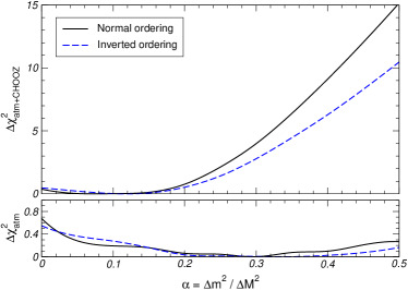
Figure 4: Dependence of the $\Delta\chi^{2}_{\rm atm}$ and $\Delta\chi^{2}_{\rm atm+CHOOZ}$ functions on the mass splitting parameter $\alpha$ for $\tan^{2}\theta_{12}=0.45$, for the analysis of atmospheric neutrinos alone (lower panel) and also in combination with the CHOOZ reactor data (upper panel).

This result can be compared with the best fit point obtained in the one–dominant mass scale approximation $\alpha=0$

$$\Delta M^{2} = 3.0\times 10^{-3}~{}{\rm eV}^{2}$$

$$\sin^{2}\theta_{23} = 0.54$$

$$\sin^{2}\theta_{13} = 0.14$$ (20)

$$\chi^{2}_{\rm atm,min} = 39.6$$

(for 62 d.o.f., one more than in the $\alpha$-unconstrained case) which is independent of the choice $\cos\delta=\pm 1$ and corresponds to Inverted schemes. Notice that this is the minimum used to obtain the allowed parameter space in the one-dominant mass scale approximation [the upper panels in Fig. 7 and the ranges in Eq. (22)], since in this case we are fixing a priori $\alpha=0$.

In summary, we find that allowing for a non-zero value of $\alpha$ very mildly improves the quality of the global fit. This result is driven by the better description of the sub-GeV data which is attainable for a non-zero $\alpha$ value, and drives the best fit point to the first octant of the mixing angle $\theta_{23}$ for which the expected number of sub-GeV electrons is larger as compared to the pure $\nu_{\mu}\rightarrow\nu_{\tau}$ scenario, as illustrated in Figs. 2 and 3. We find, however, that the analysis of the atmospheric neutrino data does not show a strong dependence on large $\alpha$ values. In the lower panel of Fig. 4 we show the dependence of $\Delta\chi^{2}_{\rm atm}$ on $\alpha$. In this plot all the neutrino oscillation parameters which are not displayed have been “integrated out”, i.e. the $\Delta\chi^{2}_{\rm atm}$ function is minimized with respect to all the non-displayed variables. From this figure we see that the fit to atmospheric neutrinos is only weakly sensitive to the value of $\alpha$.

In Fig. 5 we present sections of the allowed volume in the plane $(\cos\delta\sin^{2}\theta_{23},~{}\Delta M^{2})$ for different values of $\sin^{2}\theta_{13}$ and for values of $\Delta m^{2}=0$ (first row) and $\Delta m^{2}=3\times 10^{-4}~{}$eV² (second row) which is the (maximum allowed value by the present analysis of solar neutrino data including the latest 1496 days of SK and and day-night spectrum of SNO data 2solour . For illustration we also show the corresponding regions for the “democratic” scenario $\alpha=0.5$ ($\Delta m^{2}=\Delta M^{2}/2$). We display the corresponding sections for the Normal and Inverted schemes.

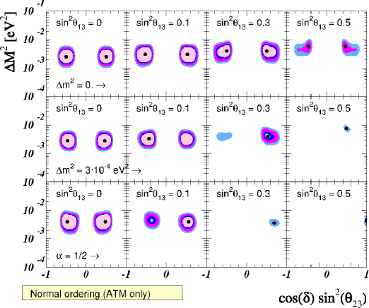
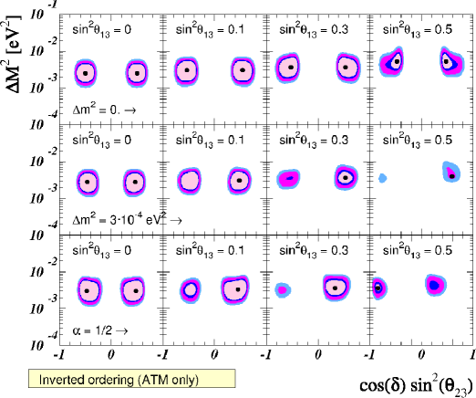
Figure 5: 90%, 95%, 99% and $3\sigma$ (4 d.o.f.) allowed regions in the $(\sin^{2}\theta_{23},\Delta M^{2})$ plane, for different values of $\sin^{2}\theta_{13}$ and $\Delta m^{2}$, from the analysis of the atmospheric neutrino data. The global minimum used to define the allowed regions is given in Eq. (19); the local minima are marked with a dot.

Comparing the sections in Fig. 5 for $\alpha=0$ with the corresponding sections for non vanishing $\alpha$ values we find that substantial differences appear although mainly for large values of $\theta_{13}$. However from these figures one also realizes that even for large values of $\alpha$ the allowed region does not extend to a very different range of $\Delta M^{2}$. Conversely, the mixing angles $\theta_{23}$ and $\theta_{13}$ can become less constrained when the case $\alpha\neq 0$ is considered.

To further quantify these effects we plot in Fig. 6 the dependence of $\Delta\chi^{2}_{\rm atm}$ on $\Delta M^{2}$, $\theta_{23}$ and $\theta_{13}$, respectively, for different values of $\alpha$, after minimizing with respect to all the non-displayed variables. From these figures we can read the $3\sigma$ allowed ranges for the different parameters (1 d.o.f.):

• For arbitrary $\alpha$

  Normal Inverted

  $$1.3\leq\frac{\Delta M^{2}}{10^{-3}~{}{\rm eV^{2}}}\leq 8.1$$

  (21)

• For $\alpha=0$ (no dependence on $\cos\delta$)

  Normal Inverted

  $$1.3\leq\frac{\Delta M^{2}}{10^{-3}~{}{\rm eV^{2}}}\leq 8.1$$

  (22)

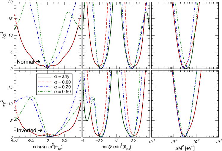
Figure 6: Dependence of the $\Delta\chi^{2}_{\rm atm}$ function on the mixing angles $\cos\delta\sin^{2}\theta_{23}$ and $\cos\delta\sin^{2}\theta_{13}$ and on the large mass scale $\Delta M^{2}$, for different values of $\alpha$ and for the Normal (upper panels) and Inverted (lower panels) cases. See text for details.

Comparing the ranges in Eqs. (21) and (22) we see that the parameter which is less sensitive to the departure from the one mass scale dominance approximation is $\Delta M^{2}$, while $\sin^{2}\theta_{13}$ is the mostly affected, in particular for the Inverted scheme for which no upper bound on $\sin^{2}\theta_{13}$ is derived from the analysis. The careful reader may notice that for the Normal ordering, the bound on $\theta_{13}$ for arbitrary $\alpha$ can be stronger than for $\alpha=0$. This is due to the fact that the ranges in Eqs. (21) and (22) are defined in terms of $3\sigma$ shifts in the $\chi^{2}$ function with respect to the minima in Eqs. (19) and (20) respectively [see explanation below Eq. (20)].

Finally we show in Fig. 7 the 2-dimensional allowed regions in $(\cos\delta\sin^{2}\theta_{23},\Delta M^{2})$ from the analysis of the atmospheric neutrino data independently of the values of $\alpha$ and $\theta_{13}$. In constructing these regions for each value of $\Delta M^{2}$ and $\cos\delta\sin^{2}\theta_{23}$ we have minimized on the oscillation parameters $\Delta m^{2}$ and $\theta_{13}$ so the they are defined in terms of $\Delta\chi^{2}$ for 2 d.o.f. ($\Delta\chi^{2}=4.61$, $5.99$, $9.21$, $11.8$ for 90%, 95%, 99% CL and $3\sigma$ respectively). For the sake of comparison we show in the figure the corresponding regions for $\alpha=0$. From the figure we see that the differences are larger for the Inverted scheme.

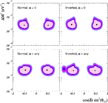
Figure 7: 90%, 95%, 99% and $3\sigma$ (2 d.o.f.) allowed regions in the $(\cos\delta\sin^{2}\theta_{23},\Delta M^{2})$ plane from the analysis of the atmospheric neutrino data, for the Normal (left panels) and Inverted (right panels) cases, for $\tan^{2}\theta_{12}=0.45$ and for arbitrary values of $\theta_{13}$ and $\alpha$ (lower panels). See text for details. The upper panels correspond to the case $\alpha=0$. The best fit point in each case is marked with a star. The local minima are marked with a dot.

4 Analysis of CHOOZ Data

The CHOOZ experiment CHOOZ searched for disappearance of $\bar{\nu}_{e}$ produced in a power station with two pressurized-water nuclear reactors with a total thermal power of $8.5$ GW (thermal). At the detector, located at $L\simeq 1$ Km from the reactors, the $\bar{\nu}_{e}$ reaction signature is the delayed coincidence between the prompt ${\rm e^{+}}$ signal and the signal due to the neutron capture in the Gd-loaded scintillator. Their measured vs. expected ratio, averaged over the neutrino energy spectrum is

$$R=1.01\pm 2.8\,\%({\rm stat})\pm 2.7\,\%({\rm syst})\,.$$ (23)

Thus no evidence was found for a deficit of measured vs. expected neutrino interactions, and they derive from the data exclusion plots in the plane of the oscillation parameters $(\Delta m^{2},\,\sin^{2}2\theta)$ in the simple two-neutrino oscillation scheme. At 90% CL they exclude the region given approximately by $\Delta m^{2}>7\cdot 10^{-4}~{}$eV² for maximum mixing, and by $\sin^{2}(2\theta)>0.10$ for large $\Delta m^{2}$. Similar searches have been performed at the Palo Verde Reactor Experiment paloverde leading to slightly weaker bounds.

In order to combine the CHOOZ bound with the results from our analysis of atmospheric neutrino data in the framework of three-neutrino mixing we have first performed our own analysis of the CHOOZ data. Using as experimental input their measured ratio (23) CHOOZ and comparing it with the theoretical expectations we define the $\chi^{2}_{\rm CHOOZ}$ function. We verified that with our $\chi^{2}_{\rm CHOOZ}$ function and using the statistical criteria for two degrees of freedom we reproduce the excluded regions given in Ref. CHOOZ as can be seen in the upper row of Fig. 8 As discussed in Sec. 2 for the analysis of the reactor data the relevant oscillation probability depends in general on the four parameters $\theta_{12}$, $\Delta m^{2}$, $\theta_{13}$, and $\Delta M^{2}$. In Fig. 8 we show the excluded regions at 90, 95 and 99% CL and $3\sigma$ in the $(\sin^{2}\theta_{13},\Delta M^{2})$ plane from our analysis of the CHOOZ data for several values of $\Delta m^{2}$ and $\tan^{2}\theta_{12}=0.45$; for the sake of comparison with the 2-family analysis we have defined the allowed regions for 2 d.o.f. ($\Delta\chi^{2}_{\rm CHOOZ}=4.61$, $5.99$, $9.21$, $11.83$ respectively). In the left (right) panel we show the results for the Normal (Inverted) scheme. We see that the presence of a non-vanishing value of $\Delta m^{2}$ results into a slightly smaller allowed range of $(\Delta M^{2},\sin^{2}\theta_{13})$. For the chosen value of $\tan^{2}\theta_{12}$ the reduction for smaller values of $\Delta M^{2}$ is slightly more significant for the Normal than for the Inverted scheme as also shown in Ref. choozpetcov . This can be easily understood from the expression of the survival probability: from Eq. (2), we get

$$P_{ee,\rm NOR}^{\rm CHOOZ}-P_{ee,\rm INV}^{\rm CHOOZ} = -\sin^{2}2\theta_{13}(\cos^{2}\theta_{12}-\sin^{2}\theta_{12})$$

$$\left[\sin^{2}\left(\frac{\Delta M^{2}L}{4E_{\nu}}\right)\right. - \left.\sin^{2}\left(\frac{(\Delta M^{2}-\Delta m^{2})L}{4E_{\nu}}\right)\right]$$ (24)

Thus for $\theta_{12}\leq\frac{\pi}{4}$ the survival probability is smaller for the Normal ordering than for the Inverted one, which leads to the stronger constraint. For $\Delta M^{2}\gg\Delta m^{2}$, Eq. (24) vanishes and the excluded regions in the two schemes become indistinguishable.

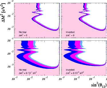
Figure 8: 90%, 95%, 99% and $3\sigma$ (2 d.o.f.) allowed regions from the analysis of the CHOOZ reactor data in the $(\sin^{2}\theta_{13},\,\Delta M^{2})$ plane for different values of $\Delta m^{2}$ ($\tan^{2}\theta_{12}=0.45$), for the Normal (left panels) and Inverted (right panels) cases.

5 Combined Analysis

We now describe the effect of including the CHOOZ reactor data together with the atmospheric data samples in a combined 3-neutrino $\chi^{2}$ analysis. The results of this analysis are summarized in the upper panel of Fig. 4 and in Figs. 9–10. As in Sec. 3, in most of results shown here we fix the mixing angle $\tan^{2}\theta_{12}=0.45$ and study how the allowed ranges of the parameters $\Delta M^{2}$ , $\sin^{2}\theta_{23}$ and $\sin^{2}\theta_{13}$ depend on $\alpha$.

We find that, in this case, the best fit point for the combined analysis of atmospheric and CHOOZ data is practically insensitive to the choice of Normal or Inverted schemes and:

$$\Delta M^{2} = 2.8\times 10^{-3}~{}{\rm eV^{2}}$$

$$\sin^{2}\theta_{23} = 0.46$$

$$\sin^{2}\theta_{13} = 0.$$ (25)

$$\Delta m^{2} = 2.8\times 10^{-4}~{}{\rm eV^{2}}\quad(\alpha=0.1)$$

$$\chi^{2}_{\rm atm+CHOOZ,min} = 39.8$$

for 62 d.o.f. and $\cos\delta=\pm 1$. Notice than in our analysis the CHOOZ data adds only one data point. Note that the point given in Eq. (25) is the global minimum used in the construction of the $\Delta\chi^{2}_{\rm atm+CHOOZ}$ function shown in Figs. 4 and 9, of the allowed regions in the lower panels of Fig. 10, and in the ranges in Eq. (27).

For $\alpha=0$ the best fit point is at:

$$\Delta M^{2} = 2.5\times 10^{-3}~{}{\rm eV^{2}}$$

$$\sin^{2}\theta_{23} = 0.49\,(\sim 0.51)$$

$$\sin^{2}\theta_{13} = 0.005$$ (26)

$$\chi^{2}_{\rm atm+CHOOZ,min} = 40.2$$

for 63 d.o.f. This is the minimum used to obtained the allowed parameters in the one-dominant mass scale approximation: the upper panels in Fig. 10 and the ranges in Eq. (28).

In the upper panel of Fig. 4 we show the dependence of $\Delta\chi^{2}_{\rm atm+CHOOZ}$ on $\alpha$. From this figure we see that the inclusion of the CHOOZ reactor data results into a stronger dependence of the analysis on the value of $\Delta m^{2}$ (or equivalently on $\alpha$) and large values of the mass splitting hierarchy parameter become disfavoured. Also the dependence is stronger for the Normal scheme, as expected (see discussion below Eq. (24)). As a consequence the ranges of mixing parameters – which, in the analysis of atmospheric data alone, were broaden in presence of large values of $\alpha$ – are expected to become narrower with the inclusion of the CHOOZ data in the analysis.

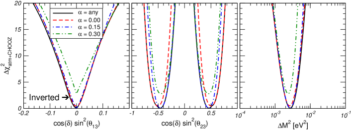
Figure 9: Dependence of the $\Delta\chi^{2}_{\rm atm+CHOOZ}$ function on the mixing angles $\cos\delta\sin^{2}\theta_{23}$ and $\cos\delta\sin^{2}\theta_{13}$ and on the large mass scale $\Delta M^{2}$, for different values of $\alpha$ and for the Inverted case. See text for details.

This effect is explicitly shown in Fig. 9, where we plot the dependence of the $\Delta\chi^{2}_{\rm atm+CHOOZ}$ on $\Delta M^{2}$, $\theta_{23}$ and $\theta_{13}$, respectively, for different values of $\alpha$ (to be compared with the corresponding Fig. 6 for the analysis of the atmospheric data). Fig. 9 is shown for the Inverted scheme. (the corresponding figure for the Normal scheme is very similar). The figure illustrates that indeed the inclusion of the CHOOZ data in the analysis results into a reduction of the allowed ranges for the mixing angles, in particular $\theta_{13}$. From this analysis we obtain the $3\sigma$ allowed (1 d.o.f.) bounds:

• For arbitrary $\alpha$

  Normal Inverted

  $$1.3\leq\frac{\Delta M^{2}}{10^{-3}~{}{\rm eV^{2}}}\leq 5.4$$

  (27)

• For $\alpha=0$

  Normal Inverted

  $$1.3\leq\frac{\Delta M^{2}}{10^{-3}~{}{\rm eV^{2}}}\leq 5.1$$

  (28)

Comparing with the results in Eq. (21) we see that including the CHOOZ reactor data reduces the effect on the final allowed range of parameters arising from allowing departures from the one mass scale dominance approximation. In other words the ranges in Eq. (27) and (28) are not very different.

Fig. 10 shows the global 2-dimensional allowed regions in ($\cos\delta\sin^{2}\theta_{23},\Delta M^{2}$) from the analysis of the atmospheric neutrino and CHOOZ reactor data for optimized values $\alpha$ and $\theta_{13}$ as well as the results for the one mass scale dominance approximation $\alpha=0$ case. Comparison with Fig. 7 shows that after including the CHOOZ reactor data the allowed range of parameters $\Delta M^{2}$ and $\sin^{2}\theta_{23}$ becomes more “robust” and it is almost independent of the Normal or Inverted ordering of the masses or of the particular choice of $\cos\delta=\pm 1$.

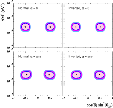
Figure 10: 90%, 95%, 99% and $3\sigma$ (2 d.o.f.) allowed regions in the $(\cos\delta\sin^{2}\theta_{23},\Delta M^{2})$ plane, from the analysis of the atmospheric and CHOOZ neutrino data with $\tan^{2}\theta_{12}=0.45$, for the Normal (left panels) and Inverted (right panels) cases and for arbitrary values of $\theta_{13}$ and $\alpha$ (lower panels). See text for details. The upper panels correspond to the case $\alpha=0$. The best fit point in each case is marked with a star. The local minima are marked with a dot.

How large would have $\alpha$ and/or $\theta_{13}$ to be for 3–$\nu$ effects to be visible in the global analysis?. We find that in order to have a 3$\sigma$ effect on the global analysis either $\tan^{2}\theta_{13}$ should be larger than $0.07$ or $\alpha$ should be larger than 0.4.

6 Summary

In this article we have explored the effect of keeping the two mass scales on the three–flavour oscillation analysis of the atmospheric and reactor neutrino data. First we have performed the independent analyses of the atmospheric neutrino data and of the CHOOZ data. We have studied the allowed parameter space resulting from these analyses as a function of the mass splitting hierarchy parameter $\alpha=\Delta m^{2}/\Delta M^{2}$ which parametrizes the departure from the one–dominant mass scale approximation. Finally we have studied the effect of keeping the two mass scales on the combined analysis.

In general the analysis of atmospheric data involves six parameters: two mass differences, which we denote by $\Delta M^{2}$ and $\Delta m^{2}$, three mixing angles ($\theta_{23}$, $\theta_{13}$ and $\theta_{12}$) and one CP phase ($\delta$). The analysis of the reactor data involves four of these parameters, namely, $\Delta M^{2}$ and $\delta m^{2}$, $\theta_{13}$ and $\theta_{12}$. For the sake of simplicity we have concentrated on the dependence on $\Delta m^{2}$ while keeping the CP phase fixed to CP conserving values and the mixing angle $\theta_{12}$ to be within the LMA range favoured in the global analysis of solar neutrino data by choosing a characteristic value $\tan^{2}\theta_{12}=0.45$. We have verified that the atmospheric data alone or in combination with the CHOOZ data is not sensitive enough to give any constraint on the possibility of CP violation nor to variations of the $\tan^{2}\theta_{12}$ within the allowed LMA range. Thus our conclusions are robust.

Our results can be summarized as follows:

• The dominant effect of a non-vanishing value of $\alpha$ in the atmospheric neutrino events is an increase (decrease) of the expected number of contained $\nu_{e}$ for $\theta_{23}$ in the first (second octant) as previously discussed in Refs. smirnov1 ; smirnov2 .

• In the predicted atmospheric neutrino events the effects of a non-vanishing $\alpha$ and of the mixing angle $\theta_{13}$ can have opposite signs and certain degree of cancellation may occur between both effects.

• The survival probability of $\bar{\nu}_{e}$ at CHOOZ decreases for increasing values of $\theta_{13}$ and $\alpha$, so that the effect of both parameters is additive in the CHOOZ reactor data. For $\theta_{12}\leq\frac{\pi}{4}$ the effect of $\Delta m^{2}$ is slightly stronger for the Normal mass ordering choozpetcov ; irina .

• Allowing for a non-zero value of $\alpha$ very mildly improves the quality of the atmospheric neutrino fit as a consequence of the better description of the sub-GeV electron data. This effect drives the best fit point to the first octant of the mixing angle $\theta_{23}$.

• Still the fit to atmospheric neutrinos is very insensitive to large values of $\alpha$ as long as all other parameters are allowed to vary accordingly.

• As a consequence the allowed range of $\sin^{2}\theta_{13}$ and $\sin^{2}\theta_{23}$ from the atmospheric neutrino data analysis becomes, in general, broader than the one for the $\alpha=0$ case.

• On the other hand the allowed range of $\Delta M^{2}$ obtained from the atmospheric neutrino data fit is stable under departures from the one mass scale dominance approximation.

• The inclusion of the CHOOZ reactor data in the analysis leads to a stronger dependence of the results on the value of $\alpha$, with smaller values of $\alpha$ and $\theta_{13}$ favoured.

• As a consequence the final determination of the allowed ranges for both $\Delta M^{2}$ and the mixing angles $\theta_{23}$ and $\theta_{13}$ is very robust and the ranges are only slightly different from those obtained in the one mass scale dominance approximation.

- (1) Y. Fukuda et al., Phys. Lett. B433, (1998) 9; Phys. Lett. B436, (1998) 33 ; Phys. Lett. B467, (1999) 185 ; Phys. Rev. Lett. 82, (1999) 2644.
- (2) M.Shiozawa, SuperKamiokande Coll., in XXth International Conference on Neutrino Physics and Astrophysics, Munich May 2002, (http://neutrino2002.ph.tum.de).
- (3) S. Fukuda et al. [Super-Kamiokande Collaboration], hep-ex/0205075.
- (4) SNO Collaboration, Q. R. Ahmad et al. Phys. Rev. Lett. 87,(2001) 071301.
- (5) SNO collaboration, Q.R. Ahmad et al. et al., nucl-ex/0204008; nucl-ex/0204009;
- (6) B. T. Cleveland et al., Astrophys. J. 496, (1998) 505.
- (7) SAGE Collaboration, J. N. Abdurashitov et al., Phys. Rev. C60, (1999) 055801.
- (8) GALLEX Collaboration, W. Hampel et al., Phys. Lett. B447, (1999) 127;
- (9) T. Kirsten, GNO Collaboration, talk at XX International Conference on Neutrino Physics and Astrophysics, Munich, Germany, May 2002 (http://neutrino2002.ph.tum.de).
- (10) J. N. Bahcall, N. A. Bahcall and G. Shaviv, Phys. Rev. Lett. 20, (1968) 1209 ; J. N. Bahcall and R. Davis, Science 191, (1976)264.
- (11) For a recent review see M.C. Gonzalez-Garcia and Y. Nir, hep-ph/0202058.
- (12) B. Pontecorvo, J. Exptl. Theoret. Phys. 33, 549 (1957) [Sov. Phys. JETP 6, 429 (1958)]; Z. Maki, M. Nakagawa and S. Sakata, Prog. Theo. Phys. 28, (1962) 870 ; M. Kobayashi and T. Maskawa, Prog. Theor. Phys. 49, (1973) 652;
- (13) S. M. Bilenky, J. Hosek and S. T. Petcov, Phys. Lett. B 94, 495 (1980).
- (14) Particle Data Group, D. E. Groom et al., Eur. Phys. J.C15, (2000) 1.
- (15) J. N. Bahcall, M. C. Gonzalez-Garcia and C. Pena-Garay, JHEP 0108, (2001) 014; hep-ph/0204314.
- (16) G. L. Fogli, E. Lisi, D. Montanino and A. Palazzo, Phys. Rev. D 64, (2001) 093007; A. Bandyopadhyay, S. Choubey, S. Goswami and K. Kar, Phys. Lett. B 519, (2001) 83; A. Bandyopadhyay, S. Choubey, S. Goswami and D. P. Roy, hep-ph/0204286; P. Krastev and A. Y. Smirnov Phys. Rev. D 65, (2002) 073022; P. C. de Holanda and A. Y. Smirnov, hep-ph/0205241. M. V. Garzelli, and C. Giunti Phys. Rev. D 65 (2002) 093005; Creminelli,P., G. Signorelli, and A. Strumia, JHEP 0105, (2001) 052; V. Barger, D. Marfatia, K. Whisnant and B. P. Wood, Phys. Rev. Lett. 88 (2002) 011302; hep-ph/0204253.
- (17) N. Fornengo, M. C. Gonzalez-Garcia and J. W. F. Valle, Nucl. Phys. B580 (2000) 58; R. Foot, R.R. Volkas and O. Yasuda, Phys. Rev. D58, (1998) 013006; O. Yasuda, Phys. Rev. D58, (1998) 091301; E.Kh. Akhmedov, A. Dighe, P. Lipari and A.Yu. Smirnov, Nucl. Phys. B542, (1999) 3.
- (18) G.L. Fogli, E. Lisi and A. Marrone, Phys. Rev. D 64, (2001) 093005.
- (19) M. C. Gonzalez-Garcia, M. Maltoni, C. Pena-Garay and J. W. Valle, Phys. Rev. D 63, (2001) 033005.
- (20) G. L. Fogli, E. Lisi, A. Maronne and G. Scioscia, Phys. Rev. D59, (1999) 033001; G.L. Fogli, E. Lisi, D. Montanino and G. Scioscia Phys. Rev. D55, (1997) 4385 ; A. De Rujula, M.B. Gavela, P. Hernandez, Phys. Rev. D63, (2001) 033001; T. Teshima, T. Sakai, Phys. Rev. D 62, (2000)113010.
- (21) G.L. Fogli, E. Lisi, D. Montanino, Phys. Rev. D54, (1996) 2048; G. L. Fogli, E. Lisi, D. Montanino and A. Palazzo, Phys. Rev. D62, (2000) 113004 ; A.M. Gago, H. Nunokawa, R. Zukanovich Funchal; Phys. Rev. D 63, (2001) 013005.
- (22) M. Apollonio, et al., CHOOZ Coll., Phys. Lett. B 466, (1999)415.
- (23) S. M. Bilenky, D. Nicolo and S. T. Petcov, hep-ph/0112216; S. T. Petcov and M. Piai, hep-ph/0112074.
- (24) I. Mocioiu and R. Shrock, JHEP 0111, (2001) 050.
- (25) O. L. Peres and A. Y. Smirnov, Phys. Lett. B 456, 204 (1999).
- (26) O. L. Peres and A. Y. Smirnov, Nucl. Phys. Proc. Suppl. 110 (2002) 355.
- (27) A. Strumia, JHEP 04, (1999) 26.
- (28) M. Narayan and S. Uma Sankar, hep-ph/0111108.
- (29) A. Marrone, talk at the NOON 2001 workshop, (http://www-sk.icrr.u-tokyo.ac.jp/noon2001).
- (30) M.Ambrosio et al., MACRO Coll., Phys. Lett. B 517, (2001) 59; M. Goodman, XXth International Conference on Neutrino Physics and Astrophysics, Munich May 2002. (http://neutrino2002.ph.tum.de).
- (31) L. Wolfenstein, Phys. Rev. D17, (1978) 2369; S. P. Mikheev and A. Y. Smirnov, Sov. J. Nucl. Phys. 42 (1985) 913 [Yad. Fiz. 42 (1985) 1441].
- (32) J. Gluza and M. Zralek, Phys. Lett. B 517, (2001) 158.
- (33) J. Schechter and J. W. F. Valle, Phys. Rev. D24, 1883 (1981) and Phys. Rev. D25, (1982) 283 ; L. Wolfenstein, Phys. Lett. B107, (1981) 77.
- (34) E. Lisi and D. Montanino, Phys. Rev. D56, (1997) 1792.
- (35) A.M. Dziewonski and D.L. Anderson, Phys. Earth Planet. Inter. 25, (1981) 297.
- (36) M. Chizhov, M. Maris and S. T. Petcov, hep-ph/9810501.
- (37) A. Piepke [Palo Verde Collaboration], Prog. Part. Nucl. Phys. 48 (2002) 113.