The Vector Meson Form Factor Analysis in Light-Front Dynamics

Abstract

We study the form factors of vector mesons using a covariant fermion field theory model in $(3+1)$ dimensions. Performing a light-front calculation in the $q^{+}=0$ frame in parallel with a manifestly covariant calculation, we note the existence of a nonvanishing zero-mode contribution to the light-front current $J^{+}$ and find a way of avoiding the zero-mode in the form factor calculations. Upon choosing the light-front gauge ($\epsilon^{+}_{h=\pm}=0$) with circular polarization and with spin projection $h=\uparrow\downarrow=\pm$, only the helicity zero to zero matrix element of the plus current receives zero-mode contributions. Therefore, one can obtain the exact light-front solution of the form factors using only the valence contribution if only the helicity components, $(h^{\prime}h)=(++),(+-)$, and $(+0)$, are used. We also compare our results obtained from the light-front gauge in the light-front helicity basis (i.e. $h=\pm,0$) with those obtained from the non-LF gauge in the instant form linear polarization basis (i.e. $h=x,y,z$) where the zero-mode contributions to the form factors are unavoidable.

I Introduction

One of the great challenges in hadronic physics is to calculate the structure of hadrons starting from QCD alone. Presently this task is very difficult and one relies on specific models to gain some understanding of hadronic structure at low energies and momentum transfer values. A popular model is the constituent quark model (CQM) which in its relativized form has met with quite some success. A first test of this model is the comparison of the mass spectra it predicts to the experimental data. Such a test provides some constraints on the wave functions. A more stringent test for the wave functions is found when one also calculates the form factors of a hadron. It lies in the nature of the CQM that only valence wave functions are determined easily. However, in a fully covariant calculation of the form factors one needs the full structure of the hadron-quark vertex.

It has been known for some time that there are situations where the form factors can be expressed correctly as convolutions of the wave functions. Such is the case for certain components of the currents. In particular one finds within the formalism of light-front dynamics (LFD) [1] that the so-called plus component of the currents for a scalar or pseudoscalar meson can be expressed in terms of the wave functions alone for spacelike momentum transfer. The matrix elements obtained this way we call the valence parts. The parts arising from vertices that can not be expressed in the wave functions we call the nonvalence parts. (The plus component of a four-vector being a particular combination of its usual components: $p^{+}=(p^{0}+p^{3})/\sqrt{2}$ where the factor $\sqrt{2}$ is conventional.)

In the case of vector mesons the situation is more complicated. Till now there have been several recipes [2, 3, 4] for the extraction of the invariant form factors from the matrix elements of the currents. It turns out that even when one limits oneself to the plus component, these different ways of extracting the form factors do not produce the same results [5]. One realizes that since the nine complex matrix elements of the current($J^{+}$), corresponding to the possible combinations of the polarizations of the initial and final spin-1 particles, can be expressed in terms of three real invariants only, it becomes clear that there must be relations between these matrix elements. This was of course known for a long time and many authors have used this knowledge to sort out the invariants from the calculated matrix elements. In reference frames where the plus-component of the momentum transfer, $q^{+}$, vanishes these relations can be reduced to just one besides the relations provided by Hermiticity, parity and rotation about the $z$-axis. The latter relation is known as the angular condition [2]. In general reference frames the situation was not so clear. In a previous paper [6] we completely analyzed these conditions for the spin-1 case and found besides the angular condition given before another one. There we gave only the formal expressions for these consistency conditions. In the $q^{+}=0$ frame, however, the additional condition is very simple involving only two helicity amplitudes and doesn’t seem to provide as strong a constraint as the usual condition since most constituent quark models are expected to satisfy it rather easily. Nevertheless, the $q^{+}=0$ frame is in principle restricted to the spacelike region of the form factors and it may be useful to impose this additional condition in processes involving the timelike region which must be analyzed in the $q^{+}\neq 0$ frame. Thus, it is important to analyze both angular conditions in different frames calculating actually the form factors with existing theoretical models. In the present paper, we demonstrate their usefulness for theoretical/phenomenological models for spin-1 objects. In order that the matrix elements satisfy these constraints, the current operator must transform properly and the state vectors must be eigenstates of total spin. If the models do not have these properties, the angular conditions will not be met.

In this work, we use a simple but exactly solvable model for the spin-1 (e.g. $\rho$) meson and separate the valence and nonvalence contributions to the three physical form factors to investigate the degree of violations in the two angular conditions for each contribution in different frames. Although the quantitative results that we find in this model may differ in other models depending on the details of the dynamics in each model, the basic structure of model calculations is common and we expect the essential findings from this model calculation may apply to realistic models.

In particular, we compared two different types of polarization vectors, the one obtained from the LF gauge ($\epsilon^{+}_{h=\pm}=0)$, which is usually used in the LF CQM analysis, and the other obtained from the instant form (IF) polarization, which is not associated with the LF gauge, i.e. $\epsilon^{+}_{x}\neq 0$, but used in some recent papers[7, 8, 9]. In both cases, there is a zero-mode contribution, i.e. a contribution from the nonvalence part that remains finite for $q^{+}\to 0$, even if the plus-component of the currents is used. Specifically, there is a zero mode contribution in the LF helicity case ($h=+,-,0$) to the $(h^{\prime},h)=(0,0)$ amplitude, where $h$ and $h^{\prime}$ are the initial and final helicities, respectively, but there is no zero-mode for other helicity combinations such as $(+,+),(+,-)$ and $(+,0)$. On the other hand, in the instant form case, only $(yy)$ is immune to the zero-mode but others such as $(xx),(zz)$ and $(zx)$ do receive zero-mode contributions. Of course, the two results are exactly the same if one properly includes the zero-mode contribution.

Now turning to the angular conditions, there are several different prescriptions [2, 3, 4] in choosing the matrix elements to extract the three physical form factors. We compare three different types of helicity combinations, GK[2], CCKP[3], and BH [4], using both LF and instant form helicity bases in a reference frame where $q^{+}=0$. One of our very interesting findings of the analysis in the LF helicity basis is that the prescription using the plus-component of the current but not involving the $(h^{\prime},h)=(0,0)$ helicity amplitude in the LF gauge is preferred for model calculation. Especially, the GK prescription uses only $(h^{\prime},h)=(+,+),(+,-)$ and $(+,0)$ but not the pure $(0,0)$ component and thus achieves the goal of not involving the zero-modes. On the other hand, the longitudinal (0,0) component is the most dominant contribution in the high momentum transfer region and thus it may be better to use the BH prescription, involving the $(0,0),(+,0)$ and $(+,-)$ amplitudes only, in the high momentum perturbative QCD analysis. The CCKP prescription, however, involves all helicity states, i.e. $(+,+),(0,0),(+,0)$ and $(+,-)$ and one needs a quantitative analysis of the angular conditions to pin down the momentum transfer region for the validity of this prescription. Our quantitative analyses indeed verify that the GK prescription is remarkably free from the zero-mode contribution but others are not. In the recent work by Melikhov and Simula[9], we see that the result using the GK prescription is not in complete agreement with their covariant model calculation, which is due to the dependence on a light-like four-vector called $\omega(\omega^{2}=0)$ in their formulation that necessarily involves unphysical form factors. The covariant formulation presented in our work should be intrinsically distinguished from theirs[9], since our formulation involves neither $\omega$ nor any unphysical form factor.

If we use the instant form basis, however, all three prescriptions receive the zero-mode contribution. Since the instant form helicity is not obtained from the LF gauge, i.e. $\epsilon^{+}_{x}\neq 0$, even the GK prescription gets the zero-mode contribution especially for the magnetic form factor as we shall show in this work. Thus, the instant form basis used in the LF formulation seems quite dangerous, because it can lead to a wrong interpretation of the physics involved in LF dynamical models. Our solvable model calculation clearly indicates that one can avoid the zero-mode contribution if the LF basis when the LF gauge is used without using the longitudinal to longitudinal helicity amplitude.

This paper is organized as follows. In Section II, we summarize the angular conditions for spin-1 systems using the LF helicity basis and the kinematics for the reference frames Drell-Yan-West (DWY), Breit (BRT), and target-rest frame (TRF) used in this work. The three prescriptions (GK, CCKP, BH) used in extracting the physical form factors are also briefly discussed in that Section. In Section III, we present our covariant model calculations of physical quantities such as the three electromagnetic form factors and the decay constant of the spin-1 meson system using both the manifestly covariant Feynman method and the LF technique. In the $q^{+}=0$ frame, we separate the full amplitudes into the valence contribution and the zero-mode contribution to show explicitly that only the helicity zero to zero amplitude is contaminated by the zero-mode. In Section IV, we present the numerical results for the form factors and the angular conditions and analyze the dependences on the prescriptions, reference frames, and helicity bases. The taxonomical decompositions of the full results into valence and non-valence contributions are used wherever possible to make a quantitative comparison of these dependences. Conclusions follow in Section V. The details of the instant form analysis and a derivation of the zero-mode are summarized in the Appendices A and B, respectively.

II Spin-1 form factors in light-front helicity basis

The Lorentz-invariant electromagnetic form factors $F_{1}$, $F_{2}$, and $F_{3}$ for a spin-1 particle of mass $m$ are defined [10] by the matrix elements of the currents $J^{\mu}$ between the initial $|p,h\rangle$ and the final $|p^{\prime},h^{\prime}\rangle$ eigenstates of the momentum $p$ and the helicity $h$ as follows:

$$G^{\mu}_{h^{\prime}h}=\langle p^{\prime},h^{\prime}|J^{\mu}|p,h\rangle=-\epsilon^{*}_{h^{\prime}}\cdot\epsilon_{h}(p+p^{\prime})^{\mu}F_{1}(Q^{2})+(\epsilon^{\mu}_{h}\;q\cdot\epsilon^{*}_{h^{\prime}}-\epsilon^{*\mu}_{h^{\prime}}\;q\cdot\epsilon_{h})F_{2}(Q^{2})+\frac{(\epsilon^{*}_{h^{\prime}}\cdot q)(\epsilon_{h}\cdot q)}{2m^{2}}(p+p^{\prime})^{\mu}F_{3}(Q^{2}),$$ (1)

where $Q^{2}=-q^{2}$, $q=p^{\prime}-p$ and $\epsilon_{h}(\epsilon_{h^{\prime}})$ is the polarization vector of the initial(final) meson.

The physical form factors, charge, magnetic, and quadrupole, are related in a well-known way to the form factors $F_{i}$, viz,

$$G_{C} = (1+\frac{2}{3}\eta)F_{1}+\frac{2}{3}\eta F_{2}+\frac{2}{3}\eta(1+\eta)F_{3}$$ (2)

$$G_{M} = -F_{2}$$ (3)

$$G_{Q} = F_{1}+F_{2}+(1+\eta)F_{3},$$ (4)

where $\eta=Q^{2}/(4m^{2})$.

Using the convention $\varepsilon^{\mu}=(\varepsilon^{+},\varepsilon^{-},\varepsilon^{1},\varepsilon^{2})$, the general form of the LF polarization vectors is given by

$$\left.\begin{array}[]{c}\varepsilon_{\rm LF}(p^{+},p^{1},p^{2};+)\\ \varepsilon_{\rm LF}(p^{+},p^{1},p^{2};0)\\ \varepsilon_{\rm LF}(p^{+},p^{1},p^{2};-)\end{array}\right\}=\left\{\begin{array}[]{c}\left(0,\frac{p^{r}}{p^{+}},\frac{-1}{\surd 2},\frac{-i}{\surd 2},\right)\\ \left(\frac{p^{+}}{m},\frac{\vec{p}^{\perp\,2}-m^{2}}{2mp^{+}},\frac{p^{1}}{m},\frac{p^{2}}{m}\right).\\ \left(0,\frac{p^{l}}{p^{+}},\frac{1}{\surd 2},\frac{-i}{\surd 2}\right)\end{array}\right.$$ (5)

Here $p^{r}(p^{l})=\mp(p_{x}\pm ip_{y})/\surd 2$. Using Eqs.(1) and (5), we obtain the matrix elements:

$$G^{+}_{h^{\prime}h} = \left(\begin{array}[]{ccc}G^{+}_{++}&G^{+}_{+0}&G^{+}_{+-}\\ G^{+}_{0+}&G^{+}_{00}&G^{+}_{0-}\\ G^{+}_{-+}&G^{+}_{-0}&G^{+}_{--}\end{array}\right),$$ (9)

$$= \left(\begin{array}[]{ccc}a_{1}F_{1}+a_{3}F_{3}&c_{1}F_{1}+c_{2}F_{2}+c_{3}F_{3}&e^{*}_{3}F_{3}\\ b_{1}F_{1}+b_{2}F_{2}+b_{3}F_{3}&d_{1}F_{1}+d_{2}F_{2}+d_{3}F_{3}&-(b_{1}F_{1}+b_{2}F_{2}+b_{3}F_{3})^{*}\\ e_{3}F_{3}&-(c_{1}F_{1}+c_{2}F_{2}+c_{3}F_{3})^{*}&a_{1}F_{1}+a_{3}F_{3}\end{array}\right).$$ (13)

Since we are working only with the plus component of the current, we shall use the following short-hand notations

$\displaystyle G_{a}=G^{+}_{++}=G^{+*}_{--},\quad G_{b}=G^{+}_{0+}=-G^{+*}_{0-},$

$$G_{c}=G^{+}_{+0}=-G^{+*}_{-0},\;G_{d}=G^{+}_{00},\;G_{e}=G^{+}_{-+}=G^{+*}_{+-}.$$ (14)

The invariant form factors can be extracted in a straightforward way. The simplest procedure is to solve first for $F_{3}$ from $G_{e}$. Next $F_{1}$ is obtained from $G_{a}$ and $F_{3}$. Then there are three options for obtaining $F_{2}$ from $G_{b}$, $G_{c}$, and $G_{d}$. These solutions are denoted by $F^{b}_{2}$, $F^{c}_{2}$, and $F^{d}_{2}$, respectively. The full solutions are then

$$\ F_{1} = \frac{1}{a_{1}}G_{a}-\frac{a_{3}}{a_{1}e_{3}}G_{e},$$ (15)

$$F_{3} = \frac{1}{e_{3}}G_{e},$$ (16)

$$F^{b}_{2} = \frac{1}{b_{2}}\left[-\frac{b_{1}}{a_{1}}\,G_{a}+G_{b}+\frac{a_{3}b_{1}-a_{1}b_{3}}{a_{1}e_{3}}\,G_{e}\right],$$ (17)

$$F^{c}_{2} = \frac{1}{c_{2}}\left[-\frac{c_{1}}{a_{1}}\,G_{a}+G_{c}+\frac{a_{3}c_{1}-a_{1}c_{3}}{a_{1}e_{3}}\,G_{e}\right],$$ (18)

$$F^{d}_{2} = \frac{1}{d_{2}}\left[-\frac{d_{1}}{a_{1}}\,G_{a}+G_{d}+\frac{a_{3}d_{1}-a_{1}d_{3}}{a_{1}e_{3}}\,G_{e}\right].$$ (19)

This procedure makes it clear that the covariant form factors of a spin-1 hadron in Eq. (1) can be determined using only the plus component of the currents, $G^{+}_{h^{\prime}h}(0)\equiv\langle P^{\prime},h^{\prime}|J^{\mu}|P,h\rangle$, in any chosen Lorentz frame. The nine elements of the current operator $G^{+}_{h^{\prime}h}(0)$ must be constrained by the invariance under (i) time-reversal, (ii) rotation about $\hat{z}$ and (iii) reflection in the plane perpendicular to $\hat{z}$, and rotational covariance, i.e. invariance under the rotations about an axis perpendicular to $\hat{z}$. So two additional constraints on the current operator are required. These consistency conditions are the angular conditions, which we define as [6]

$$\Delta_{\rm bc}=F^{b}_{2}-F^{c}_{2},\quad\Delta_{\rm bd}=F^{b}_{2}-F^{d}_{2}.$$ (20)

We know that the form of these conditions depends on the reference frame [6]. In this work we consider three different frames, which we define in the following subsection II A. Especially, in the frames where $q^{+}=0$, our angular condition $\Delta_{\rm bd}$ is equivalent to the usual angular condition relating the four helicity amplitudes discussed in the literature[2] modulo an overall factor as we discuss in the subsection II B.

A Kinematics

Our conventions for the momenta of the initial and final state mesons in the three different reference frames, (DYW), (BRT), and (TRF) are given below. We use the notation $p^{\mu}=(p^{+},p^{-},p_{x},p_{y})=(p^{+},p^{-},\vec{p}_{\perp})$ and the metric convention $p\cdot q=p^{+}q^{-}+p^{-}q^{+}-\vec{p}_{\perp}\cdot\vec{q}_{\perp}$.

DYW

$$p = (p^{+},m^{2}/(2p^{+}),0,0)$$ (21)

$$p^{\prime} = (p^{+},(Q^{2}+m^{2})/(2p^{+}),Q\cos\phi,Q\sin\phi)$$ (22)

BRT

$$\beta=\sqrt{1+\left(\frac{Q}{2m}\right)^{2}}.$$ (23)

$$p = \left(\frac{2m\beta-Q\cos\theta}{2\surd 2},\frac{2m\beta+Q\cos\theta}{2\surd 2},-\frac{Q\sin\theta\cos\phi}{2},-\frac{Q\sin\theta\sin\phi}{2}\right),$$ (24)

$$p^{\prime} = \left(\frac{2m\beta+Q\cos\theta}{2\surd 2},\frac{2m\beta-Q\cos\theta}{2\surd 2},\frac{Q\sin\theta\cos\phi}{2},\frac{Q\sin\theta\sin\phi}{2}\right).$$ (25)

TRF

$$\kappa=\frac{Q^{2}}{2m},$$ (26)

$$p = \left(\frac{m}{\surd 2},\frac{m}{\surd 2},0,0\right).$$ (27)

$$p^{\prime} = \left(\frac{m+\kappa+\beta Q\cos\theta}{\surd 2},\frac{m+\kappa-\beta Q\cos\theta}{\surd 2},\beta Q\sin\theta\cos\phi,\beta Q\sin\theta\sin\phi\right).$$ (28)

In the literature usually the reference frames used are limited to ones where $q^{+}=0\;(q^{2}=2q^{+}q^{-}-\vec{q}^{2}_{\perp}<0)$. One of such reference frames is the special Breit frame used in Refs. [2, 3, 4, 5, 11, 12], where $q^{+}=0,q_{y}=0,q_{x}=Q$, and $\vec{p}_{\perp}=-\vec{p^{\prime}}_{\perp}$ i.e. $\theta=\frac{\pi}{2},\phi=0$ in Eq.(25);

Special Breit

$$q^{\mu}=(0,0,Q,0),\;p^{\mu}=(m\sqrt{1+\eta}/\surd 2,m\sqrt{1+\eta}/\surd 2,-Q/2,0),\;p^{\prime\mu}=(m\sqrt{1+\eta}/\surd 2,m\sqrt{1+\eta}/\surd 2,Q/2,0),$$ (29)

where $\eta=Q^{2}/4m^{2}$ is a kinematic factor. The corresponding polarization vectors are obtained by substituting these four vectors in Eq. (5) and the transverse($h=\pm$) and longitudinal($h=0$) polarization vectors in this special Breit frame are given by

$$\epsilon^{\mu}(p,\pm)=\frac{\mp 1}{\sqrt{2}}\biggl{(}0,\frac{-Q}{2p^{+}},1,\pm i\biggr{)},\;\epsilon^{\mu}(p,0)=\frac{1}{m}\biggl{(}p^{+},\frac{-m^{2}+Q^{2}/4}{2p^{+}},\frac{-Q}{2},0\biggr{)},$$ (30)

$$\epsilon^{\mu}(p^{\prime},\pm)=\frac{\mp 1}{\sqrt{2}}\biggl{(}0,\frac{Q}{2p^{+}},1,\pm i\biggr{)},\;\epsilon^{\mu}(p^{\prime},0)=\frac{1}{m}\biggl{(}p^{+},\frac{-m^{2}+Q^{2}/4}{2p^{+}},\frac{Q}{2},0\biggr{)}.$$ (31)

B Angular condition in $q^{+}=0$ frame and prescriptions of choosing helicity amplitudes

In the $q^{+}=0$ frame, one can reduce the independent matrix elements of the current down to four, e.g. $G^{+}_{++},G^{+}_{+-},G^{+}_{+0}$ and $G^{+}_{00}$ using the front-form helicity basis [2, 3, 4, 5, 12] and the rotational covariance requires one additional constraint on the current operator. This is what these authors call the angular condition $\Delta(Q^{2})$ and can be obtained from the explicit representations of the helicity amplitudes in terms of the physical form factors. Using the relation between the covariant form factors $F_{i}$ and the current matrix elements given by Eq. (1), one can obtain the following helicity amplitudes in the $q^{+}=0$ frame

$$G^{+}_{++} = 2p^{+}(F_{1}+\eta F_{3}),\;G^{+}_{+0}=p^{+}\sqrt{2\eta}(2F_{1}+F_{2}+2\eta F_{3}),$$ (32)

$$G^{+}_{+-} = -2p^{+}\eta F_{3},\;\;G^{+}_{00}=2p^{+}\{(1-2\eta)F_{1}-2\eta F_{2}-2\eta^{2}F_{3}\}.$$ (33)

Thus, the usual angular condition relating the four helicity amplitudes is given by [2]

$$\Delta(Q^{2})=(1+2\eta)G^{+}_{++}+G^{+}_{+-}-\sqrt{8\eta}G^{+}_{+0}-G^{+}_{00}=0,$$ (34)

where we note an overall factor difference between $\Delta(Q^{2})$ and $\Delta_{bd}(Q^{2})$, i.e. $\Delta=d_{2}\Delta_{bd}$ (See Section IV B 5 for the discussion of the factor $d_{2}$.).

In a practical computation, instead of calculating the Lorentz-invariant form factors $F_{i}(Q^{2})$, the physical charge ($G_{C}$), magnetic ($G_{M}$), and quadrupole ($G_{Q}$) form factors are often used. However, the relations between the physical invariant form factors and the matrix elements $G^{+}_{h^{\prime}h}$ [5] are not unique. Only if the matrix elements fulfill the angular condition Eq. (34) the extracted form factors would not depend on the choice made. So one may choose which matrix elements to use to extract the form factors. Perhaps the most popular choices are [2, 3, 4]:

$$G_{C}^{\rm GK} = \frac{1}{2p^{+}}\biggl{[}\frac{(3-2\eta)}{3}G^{+}_{++}+\frac{4\eta}{3}\frac{G^{+}_{+0}}{\sqrt{2\eta}}+\frac{1}{3}G^{+}_{+-}\biggr{]},$$ (35)

$$G_{M}^{\rm GK} = \frac{2}{2p^{+}}\biggl{[}G^{+}_{++}-\frac{1}{\sqrt{2\eta}}G^{+}_{+0}\biggr{]},$$ (36)

$$G_{Q}^{\rm GK} = \frac{1}{2p^{+}}\biggl{[}-G^{+}_{++}+2\frac{G^{+}_{+0}}{\sqrt{2\eta}}-\frac{G^{+}_{+-}}{\eta}\biggr{]},$$ (37)

$$G_{C}^{\rm CCKP} = \frac{1}{2p^{+}(1+\eta)}\biggl{[}\frac{3-2\eta}{6}(G^{+}_{++}+G^{+}_{00})+\frac{10\eta}{3}\frac{G^{+}_{+0}}{\sqrt{2\eta}}+\frac{4\eta-1}{6}G^{+}_{+-}\biggr{]},$$ (38)

$$G_{M}^{\rm CCKP} = \frac{1}{2p^{+}(1+\eta)}\biggl{[}G^{+}_{++}+G^{+}_{00}-G^{+}_{+-}-\frac{2(1-\eta)}{\sqrt{2\eta}}G^{+}_{+0}\biggr{]},$$ (39)

$$G_{Q}^{\rm CCKP} = \frac{1}{2p^{+}(1+\eta)}\biggl{[}-\frac{1}{2}(G^{+}_{++}+G^{+}_{00})+2\frac{G^{+}_{+0}}{\sqrt{2\eta}}-\frac{(\eta+2)}{2\eta}G^{+}_{+-}\biggr{]},$$ (40)

and

$$G_{C}^{\rm BH} = \frac{1}{2p^{+}(1+2\eta)}\biggl{[}\frac{(3-2\eta)}{3}G^{+}_{00}+\frac{16\eta}{3}\frac{G^{+}_{+0}}{\sqrt{2\eta}}+\frac{2(2\eta-1)}{3}G^{+}_{+-}\biggr{]},$$ (41)

$$G_{M}^{\rm BH} = \frac{2}{2p^{+}(1+2\eta)}\biggl{[}G^{+}_{00}-G^{+}_{+-}+\frac{(2\eta-1)}{\sqrt{2\eta}}G^{+}_{+0}\biggr{]},$$ (42)

$$G_{Q}^{\rm BH} = \frac{1}{2p^{+}(1+2\eta)}\biggl{[}2\frac{G^{+}_{+0}}{\sqrt{2\eta}}-G^{+}_{00}-\frac{(1+\eta)}{\eta}G^{+}_{+-}\biggr{]}.$$ (43)

The relation between $F^{\prime}s$ and $G^{\prime}s$ given by Eq. (4) holds for any prescription given above.

It is interesting to note that while Grach and Kondratyuk in [2] regarded $G^{+}_{00}$ as the “worst” element and took care not to use it writing the relations Eq. (35), Brodsky and Hiller[4] included $G^{+}_{00}$ instead of $G^{+}_{++}$ expecting the helicity zero to zero component of the current matrix element to be the dominant one in the perturbative QCD regime. Chung et al. [3] used all four independent helicity components of the current matrix elements. On the other hand, in the instant form basis used by some authors [7, 8, 13], the independent matrix elements of the current operator are $G^{+}_{xx},G^{+}_{yy},G^{+}_{zz}$ and $G^{+}_{zx}$ and the angular condition becomes $\Delta(Q^{2})=G^{+}_{yy}-G^{+}_{zz}$. In appendix A, we show the relevant expressions for the form factors in the instant form spin basis [7, 8, 13]. Although the authors in Refs. [7, 8, 13] argued that this basis is completely equivalent to the LF helicity basis, the relation between them, which will be discussed later, is not trivial.

III Calculation in a solvable covariant model

The solvable model, based on the covariant Bethe-Salpeter(BS) model of ($3+1$)-dimensional fermion field theory, enables us to derive the form factors of a spin-1 particle exactly.

FIG. 1.: The covariant triangle diagram (a) is represented as the sum of a LF valence diagram (b) defined in the region $0<k^{+}<p^{+}$ and the nonvalence diagram (c) defined in $p^{+}<k^{+}<p^{\prime+}$. $\delta=q^{+}/p^{+}=p^{\prime+}/p^{+}-1$. The white and black blobs at the meson-quark vertices in (b) and (c) represent the LF wave-function and non-wave-function vertices, respectively. The small circles in (b) and (c) represent the (on-shell) mass pole of the quark propagator determined from the $k^{-}$-integration.

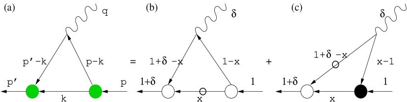
The covariant diagram shown in Fig. 1(a) is in general equivalent to the sum of the LF valence diagram (b) and the nonvalence diagram (c), where $\delta=q^{+}/p^{+}=p^{\prime+}/p^{+}-1$. The matrix element $G^{\mu}_{h^{\prime}h}(0)$ of the electromagnetic (EM) current of a spin-1 particle with equal mass constituents ($m_{q}=m_{\bar{q}}$) obtained from the covariant diagram of Fig. 1(a) is given by

$$G^{\mu}_{h^{\prime}h}(0) = iN_{c}g^{2}\int\frac{d^{4}k}{(2\pi)^{4}}\frac{S_{\Lambda}(k-p)S^{\mu}_{h^{\prime}h}S_{\Lambda}(k-p^{\prime})}{[(k-p)^{2}-m^{2}_{q}+i\varepsilon][k^{2}-m^{2}_{q}+i\varepsilon][(k-p^{\prime})^{2}-m^{2}_{q}+i\varepsilon]},$$ (44)

where $N_{c}$ is the number of colors and $g$, modulo the charge factor $e_{q}$, is the normalization constant, which can be fixed by requiring the charge form factor to be unity at zero momentum transfer. $S^{\mu}_{h^{\prime}h}$ is the trace term of the quark propagators. To regularize the covariant fermion triangle-loop in ($3+1$) dimension, we replace the point photon-vertex $\gamma^{\mu}$ by a non-local (smeared) photon-vertex $S_{\Lambda}(p)\gamma^{\mu}S_{\Lambda}(p^{\prime})$, where $S_{\Lambda}(p)=\Lambda^{2}/(p^{2}-\Lambda^{2}+i\varepsilon)$ and $\Lambda$ plays the role of a momentum cut-off similar to the Pauli-Villars regularization[1].

When we do the Cauchy integration over $k^{-}$ to obtain the LF time-ordered diagrams, we want to avoid the complexity of treating double $k^{-}$-poles, so we decompose the product of five energy denominators in Eq. (44) into a sum of terms with three energy denominators only:

$$\frac{1}{D_{\Lambda}D_{0}D_{k}D^{\prime}_{0}D^{\prime}_{\Lambda}} = \frac{1}{(\Lambda^{2}-m^{2}_{q})^{2}}\frac{1}{D_{k}}\biggl{(}\frac{1}{D_{\Lambda}}-\frac{1}{D_{0}}\biggr{)}\biggl{(}\frac{1}{D^{\prime}_{\Lambda}}-\frac{1}{D^{\prime}_{0}}\biggr{)},$$ (45)

where

$$D_{\Lambda}=(k-p)^{2}-\Lambda^{2}+i\epsilon,\;D_{0}=(k-p)^{2}-m^{2}_{q}+i\epsilon,\;D_{k}=k^{2}-m^{2}_{q}+i\epsilon,$$ (46)

and $D^{\prime}_{0[\Lambda]}=D_{0[\Lambda]}(p\to p^{\prime})$.

Our treatment of $S_{\Lambda}$ as the non-local smearing photon-vertex remedies [1] the conceptual difficulty associated with the asymmetry appearing if the fermion-loop were regulated by smearing the $q\bar{q}$ bound-state vertex. As will be discussed later, the two methods lead to different results for the calculation of the decay constant even though they give the same result for the form factors.

The vector meson decay constant $f_{V}$ in this covariant model with the nonlocal gauge boson vertex $S_{\Lambda}(k)\gamma^{\mu}S_{\Lambda}(k-p)$ is defined by

$$A^{\mu} = \langle 0|\bar{q}\gamma^{\mu}q|p;1J_{3}\rangle=i\sqrt{2}f_{V}m\epsilon^{\mu}(J_{3}),$$ (47)

where

$$A^{\mu} = N_{c}g\Lambda^{4}\int\frac{d^{4}k}{(2\pi)^{4}}\frac{{\rm Tr}[\not\!\epsilon(\not\!k-\not\!p+m_{q})\gamma^{\mu}(\not\!k+m_{q})]}{[k^{2}-m_{q}^{2}+i\varepsilon][(k-p)^{2}-m_{q}^{2}+i\varepsilon][k^{2}-\Lambda^{2}+i\varepsilon][(k-p)^{2}-\Lambda^{2}+i\varepsilon]}.$$ (48)

A Manifestly covariant calculation

In the manifestly covariant calculation, we obtain the form factors $F_{i}(i=1,2,3)$ using dimensional regularization. Although the splitting procedure Eq. (45) may not be neccessary in the covariant calculation, it seems more effective in practical computation. Here we describe some essential steps for the derivation of the covariant form factors: We $(i)$ reduce the five propagators into the sum of three propagators using Eq. (45), $(ii)$ use the Feynman parametrization for the three propagators, e.g.,

$$\frac{1}{D_{k}D_{0}D^{\prime}_{0}} = 2\int^{1}_{0}dx\int^{1-x}_{0}dy\frac{1}{[D_{k}+(D_{0}-D_{k})x+(D^{\prime}_{0}-D_{k})y]^{3}},$$ (49)

and $(iii)$ make a Wick rotation of Eq. (44) in $D$-dimension to regularize the integral, since otherwise one encounters missing the logarithmic divergent terms in Eq. (44). Following the above procedures $(i)$ -$(iii)$ we finally obtain the covariant form factors as follows:

$$F_{1}(Q^{2}) = \frac{N_{c}g^{2}\Lambda^{4}}{8\pi^{2}(\Lambda^{2}-m^{2}_{q})^{2}}\int^{1}_{0}dx\int^{1-x}_{0}dy\biggl{\{}(2-x-y){\rm ln}\biggl{(}\frac{C^{2}_{k\Lambda 0}C^{2}_{k0\Lambda}}{C^{2}_{k\Lambda\Lambda}C^{2}_{k00}}\biggr{)}$$ (51)

$$\;+\biggl{[}-(x+y)(x+y-1)^{2}m^{2}+(2-x-y)xy\;Q^{2}-(2-x-y)m^{2}_{q}\biggr{]}C^{2}\biggr{\}},$$

$$F_{2}(Q^{2}) = -\frac{N_{c}g^{2}\Lambda^{4}}{8\pi^{2}(\Lambda^{2}-m^{2}_{q})^{2}}\int^{1}_{0}dx\int^{1-x}_{0}dy\biggl{\{}(2+x+y){\rm ln}\biggl{(}\frac{C^{2}_{k\Lambda 0}C^{2}_{k0\Lambda}}{C^{2}_{k\Lambda\Lambda}C^{2}_{k00}}\biggr{)}$$ (53)

$$\;+\biggl{[}(x+y)[(x+y)^{2}-1]m^{2}+(x+y)xy\;Q^{2}-(2+x+y)m^{2}_{q}\biggr{]}C^{2}\biggr{\}},$$

$$F_{3}(Q^{2}) = \frac{N_{c}g^{2}\Lambda^{4}}{8\pi^{2}(\Lambda^{2}-m^{2}_{q})^{2}}\int^{1}_{0}dx\int^{1-x}_{0}dy\;8xy(x+y-1)m^{2}C^{2},$$ (54)

where

$$C^{2}_{k\Lambda\Lambda} = (x+y)(1-x-y)m^{2}-xy\;Q^{2}-(x+y)\Lambda^{2}-(1-x-y)m^{2}_{q},$$ (55)

$$C^{2}_{k\Lambda 0} = (x+y)(1-x-y)m^{2}-xy\;Q^{2}-(x\Lambda^{2}+ym^{2}_{q})-(1-x-y)m^{2}_{q},$$ (56)

$$C^{2}_{k0\Lambda} = C^{2}_{k\Lambda 0}(x\leftrightarrow y),$$ (57)

$$C^{2}_{k00} = (x+y)(1-x-y)m^{2}-xy\;Q^{2}-m^{2}_{q},$$ (58)

and $C^{2}=(1/C^{2}_{k\Lambda\Lambda}-1/C^{2}_{k\Lambda 0}-1/C^{2}_{k0\Lambda}+1/C^{2}_{k00})$. Note that the logarithmic terms in $F_{1}$ and $F_{2}$ are obtained from the dimensional regularization.

Following a similar procedure for the form factor calculation, the covariant result for the decay constant is obtained as

$$f^{\rm COV}_{V}=\frac{N_{c}g\Lambda^{4}}{4\sqrt{2}\pi^{2}m(\Lambda^{2}-m^{2}_{q})^{2}}\int^{1}_{0}dx \biggl{\{}[m^{2}_{q}+{\tilde{M}}^{2}]\;{\rm ln}\frac{[{\tilde{M}}^{2}-xm^{2}_{q}-(1-x)\Lambda^{2}][{\tilde{M}}^{2}-x\Lambda^{2}-(1-x)m^{2}_{q}]}{[{\tilde{M}}^{2}-\Lambda^{2}][{\tilde{M}}^{2}-m^{2}_{q}]}$$ (62)

$$\;\;-[{\tilde{M}}^{2}-\Lambda^{2}]\;\ln[-{\tilde{M}}^{2}+\Lambda^{2}]-[{\tilde{M}}^{2}-m^{2}_{q}]\;\ln[-{\tilde{M}}^{2}+m^{2}_{q}]$$

$$\;\;+[{\tilde{M}}^{2}-xm^{2}_{q}-(1-x)\Lambda^{2}]\;\ln[-{\tilde{M}}^{2}+xm^{2}_{q}+(1-x)\Lambda^{2}]$$

$$\;\;+[{\tilde{M}}^{2}-x\Lambda^{2}-(1-x)m^{2}_{q}]\;\ln[-{\tilde{M}}^{2}+x\Lambda^{2}+(1-x)m^{2}_{q}]\biggr{\}},$$

where ${\tilde{M}}^{2}=x(1-x)m^{2}$.

B Light-front calculation

We shall use only the plus-component of the current matrix element $G^{+}_{h^{\prime}h}$ in the calculation of the form factors. In principle, one can directly calculate the trace term $S^{+}_{h^{\prime}h}$ with $k^{-}=k^{-}_{\rm pole}$, which depends on the integration region of $k^{+}$. However, for the purpose of a clear understanding of the physics implied in LF dynamics, we instead separate $S^{+}_{h^{\prime}h}$ into the on-mass shell propagating part and the (off-mass shell) instantaneous one using the following identity

$$\not\!p+m_{q}=(\not\!{p_{\rm on}}+m_{q})+\gamma^{+}(p^{-}-p^{-}_{\rm on}),$$ (63)

where the subscript (on) denotes the on-mass shell ($p^{2}=m^{2}_{q}$) quark propagator, i.e. $p^{-}=p^{-}_{\rm on}=(m^{2}_{q}+\vec{p}^{2}_{\perp})/2p^{+}$. Then the trace term $S^{+}_{h^{\prime}h}$ of the quark propagators in Eq. (44) is given by

$$S^{+}_{h^{\prime}h}(P=k-p,P^{\prime}=k-p^{\prime},k)=(S^{+}_{h^{\prime}h})_{\rm on}+(S^{+}_{h^{\prime}h})_{\rm inst.},$$ (64)

where

$$(S^{+}_{h^{\prime}h})_{\rm on} = {\rm Tr}[\not\!\epsilon^{*}_{h^{\prime}}(\not\!P^{\prime}_{\rm on}+m_{q})\gamma^{+}(\not\!P_{\rm on}+m_{q})\not\!\epsilon_{h}(\not\!k_{\rm on}+m_{q})],$$ (65)

$$= \;4\;P^{+}\biggl{[}(k_{\rm on}\cdot\epsilon^{*}_{h^{\prime}})(P^{\prime}_{\rm on}\cdot\epsilon_{h})+(P^{\prime}_{\rm on}\cdot\epsilon^{*}_{h^{\prime}})(k_{\rm on}\cdot\epsilon_{h})+(\epsilon^{*}_{h^{\prime}}\cdot\epsilon_{h})(m_{q}^{2}-k_{\rm on}\cdot P^{\prime}_{\rm on})\biggr{]}$$ (70)

$$+\;4\;P^{\prime+}\biggl{[}(k_{\rm on}\cdot\epsilon^{*}_{h^{\prime}})(P_{\rm on}\cdot\epsilon_{h})+(P_{\rm on}\cdot\epsilon^{*}_{h^{\prime}})(k_{\rm on}\cdot\epsilon_{h})+(\epsilon^{*}_{h^{\prime}}\cdot\epsilon_{h})(m_{q}^{2}-k_{\rm on}\cdot P_{\rm on})\biggr{]}$$

$$+\;4\;k^{+}\biggl{[}(P^{\prime}_{\rm on}\cdot\epsilon^{*}_{h^{\prime}})(P_{\rm on}\cdot\epsilon_{h})-(P_{\rm on}\cdot\epsilon^{*}_{h^{\prime}})(P^{\prime}_{\rm on}\cdot\epsilon_{h})-(\epsilon^{*}_{h^{\prime}}\cdot\epsilon_{h})(m_{q}^{2}-P_{\rm on}\cdot P^{\prime}_{\rm on})\biggr{]}$$

$$-\;4\;\epsilon^{*+}_{h^{\prime}}\biggl{[}(P_{\rm on}\cdot\epsilon_{h})(k_{\rm on}\cdot P^{\prime}_{\rm on}-m^{2}_{q})-(P^{\prime}_{\rm on}\cdot\epsilon_{h})(k_{\rm on}\cdot P_{\rm on}-m^{2}_{q})+(k_{\rm on}\cdot\epsilon_{h})(p_{\rm on}\cdot P^{\prime}_{\rm on}-m^{2}_{q})\biggr{]}$$

$$-\;4\;\epsilon^{+}_{h}\biggl{[}(P^{\prime}_{\rm on}\cdot\epsilon^{*}_{h^{\prime}})(k_{\rm on}\cdot P_{\rm on}-m^{2}_{q})-(P_{\rm on}\cdot\epsilon^{*}_{h^{\prime}})(k_{\rm on}\cdot P^{\prime}+_{\rm on}-m^{2}_{q})+(k_{\rm on}\cdot\epsilon^{*}_{h^{\prime}})(P_{\rm on}\cdot P^{\prime}_{\rm on}-m^{2}_{q})\biggr{]},$$

and

$$(S^{+}_{h^{\prime}h})_{\rm inst.} = (k^{-}-k^{-}_{\rm on}){\rm Tr}[\not\!\epsilon^{*}_{h^{\prime}}(\not\!{P^{\prime}_{\rm on}}+m_{q})\gamma^{+}(\not\!{P_{\rm on}}+m_{q})\not\!\epsilon_{h}\gamma^{+}],$$ (71)

$$= 8(k^{-}-k^{-}_{\rm on})\biggl{[}\epsilon^{*+}_{h^{\prime}}P^{+}_{\rm on}(\epsilon_{h}\cdot P^{\prime}_{\rm on})+\epsilon^{+}_{h}P^{\prime+}_{\rm on}(\epsilon^{*}_{h^{\prime}}\cdot P_{\rm on})-P^{\prime+}_{\rm on}P^{+}_{\rm on}(\epsilon^{*}_{h^{\prime}}\cdot\epsilon_{h})+\epsilon^{*+}_{h^{\prime}}\epsilon^{+}_{h}(m^{2}_{q}-P^{\prime}_{\rm on}\cdot P_{\rm on})\biggr{]}.$$ (72)

As we shall show below, the LF valence contribution comes exclusively from the on-mass shell propagating part, Eq. (65), and the zero-mode (if it exists) from the instantaneous part, Eq. (71).

Using the special Breit frame (See Eq.(29).) with the LF gauge, we obtain for the trace terms $(S^{+}_{h^{\prime}h})_{\rm on}$ and $(S^{+}_{h^{\prime}h})_{\rm inst.}$ given by Eqs. (65) and (71) the expressions

$$(S^{+}_{++})_{\rm on} = \frac{4p^{+}}{x}\biggl{[}m^{2}_{q}+(2x^{2}-2x+1)\biggl{(}\vec{k}^{2}_{\perp}-\frac{x^{2}}{4}Q^{2}+ix(\vec{k}_{\perp}\times\vec{q}_{\perp})\cdot\hat{z}\biggr{)}\biggr{]},$$ (73)

$$(S^{+}_{+-})_{\rm on} = 8(1-x)p^{+}\biggl{[}(k_{x}-ik_{y})^{2}-\frac{x^{2}}{4}Q^{2}\bigg{]},$$ (74)

$$(S^{+}_{+0})_{\rm on} = \frac{\sqrt{8\eta}}{Q}p^{+}(2(k_{x}-ik_{y})-xQ)(2x-1)\biggl{[}(1-x)(m^{2}+M^{2}_{0})+\frac{x}{4}Q^{2}+\vec{k}_{\perp}\cdot\vec{q}_{\perp}\biggr{]},$$ (75)

$$(S^{+}_{00})_{\rm on} = \frac{4p^{+}}{m^{2}}\biggl{[}x\biggl{(}(1-x)(m^{2}+M^{2}_{0})+\frac{x}{4}Q^{2}\biggr{)}^{2}-x(\vec{k}_{\perp}\cdot\vec{q}_{\perp})^{2}\biggr{]},$$ (76)

and

$$(S^{+}_{++})_{\rm inst.} = (S^{+}_{+-})_{\rm inst.}=0,$$ (77)

$$(S^{+}_{+0})_{\rm inst.} = \frac{8(p^{+})^{2}}{m\sqrt{2}}(k^{-}-k^{-}_{\rm on})(x-1)\biggl{[}k_{x}-ik_{y}+\biggl{(}1-\frac{x}{2}\biggr{)}Q\biggr{]},$$ (78)

$$(S^{+}_{00})_{\rm inst.} = \frac{8(p^{+})^{2}}{m^{2}}(k^{-}-k^{-}_{\rm on})\biggl{[}-\frac{x^{2}}{4}Q^{2}+m^{2}_{q}+\vec{k}^{2}_{\perp}\biggr{]},$$ (79)

where $x=k^{+}/p^{+}$, and $M^{2}_{0}=(m^{2}_{q}+\vec{k}^{2}_{\perp})/[x(1-x)]$. We note that the terms proportional to an odd power of $\vec{k}_{\perp}$ do not contribute to the integral.

By doing the integration over $k^{-}$ in Eq. (44), one finds the two LF time-ordered contributions to the residue calculations corresponding to two poles in $k^{-}$, the one coming from the interval (I) $0<k^{+}<p^{+}$ (See Fig. 1(b).), the “valence diagram”, and the other from (II) $p^{+}<k^{+}<p^{\prime+}$ (See Fig. 1(c).), the “nonvalence diagram” or “Z” graph. These diagrams are expressed in terms of energy denominators.

1 Valence contribution

In the region $0<k^{+}<p^{+}$, the pole $k^{-}=k^{-}_{\rm on}=(m^{2}_{q}+\vec{k}^{2}_{\perp}-i\varepsilon)/2k^{+}$ (i.e the spectator quark), is located in the lower half of the complex $k^{-}$-plane. Thus, the Cauchy integration formula for the $k^{-}$-integral in Eq. (44) gives in this region for the plus current, $G^{+}_{h^{\prime}h}(0)$,

$$G^{+val}_{h^{\prime}h} = \frac{N_{c}}{2(2\pi)^{3}}\int^{1}_{0}\frac{dx}{x(1-x)^{4}}\int d^{2}\vec{k}_{\perp}\frac{g\Lambda^{2}}{(m^{2}-{\cal M}^{2}_{0})(m^{2}-{\cal M}^{2}_{\Lambda})}S^{+val}_{h^{\prime}h}\frac{g\Lambda^{2}}{(m^{2}-{\cal M}^{\prime 2}_{0})(m^{2}-{\cal M}^{\prime 2}_{\Lambda})},$$ (80)

where

$${\cal M}^{2}_{0} = \frac{m^{2}_{q}+(\vec{k}_{\perp}-x\vec{p}_{\perp})^{2}}{x}+\frac{m^{2}_{q}+(\vec{k}_{\perp}-x\vec{p}_{\perp})^{2}}{1-x},$$ (81)

$${\cal M}^{2}_{\Lambda} = \frac{m^{2}_{q}+(\vec{k}_{\perp}-x\vec{p}_{\perp})^{2}}{x}+\frac{\Lambda^{2}+(\vec{k}_{\perp}-x\vec{p}_{\perp})^{2}}{1-x},$$ (82)

are the invariant masses of the initial meson state. The invariant masses of the final state, i.e. ${\cal M}^{\prime 2}_{0}$ and ${\cal M}^{\prime 2}_{\Lambda}$ in Eq. (80), can be obtained by replacing $\vec{p}_{\perp}\to-\vec{p}_{\perp}$ in Eq. (81). As one can easily see from Eqs. (73) and (77), only the on-mass shell quark propagator part contributes to the valence diagram, i.e. $S^{+val}_{h^{\prime}h}=(S^{+}_{h^{\prime}h})_{\rm on}$. Note, however, that this relation does not hold in general for other components of the currents, e.g. $S^{-val}_{h^{\prime}h}\neq(S^{-}_{h^{\prime}h})_{\rm on}$. One of the distinguished features of the LF plus current matrix element given by Eq. (80) is that the physical interpretation is manifest in terms of the LF wave function, i.e. a convolution of the initial and the final state LF wave functions, which is not possible for the covariant calculation.

2 Zero-mode contribution

In the region $p^{+}<k^{+}<p^{\prime+}$, the poles are at $k^{-}=p^{\prime-}+[m^{2}_{q}+(\vec{k}_{\perp}-\vec{p^{\prime}}_{\perp})^{2}-i\varepsilon]/2(k^{+}-p^{\prime+})$ (from the struck quark propagator) and $k^{-}=p^{\prime-}+[\Lambda^{2}+(\vec{k}_{\perp}-\vec{p^{\prime}}_{\perp})^{2}-i\varepsilon]/2(k^{+}-p^{\prime+})$ (from the smeared quark-photon vertex $S_{\Lambda}(k-p^{\prime})$), and are located in the upper half of the complex $k^{-}$-plane.

Since the integration range of the nonvalence region, $p^{+}<k^{+}<p^{\prime+}(=p^{+}+q^{+})$, shrinks to zero in the $q^{+}\to 0$ limit, the nonvalence contribution is sometimes mistakenly thought to be always vanishing for $q^{+}\to 0$. However, in reality it may not vanish but give a finite contribution,

$$\lim_{q^{+}\to 0}\int^{p^{+}+q^{+}}_{p^{+}}dk^{+}(\cdots)\equiv\lim_{\delta\to 0}\int^{1+\delta}_{1}dx(\cdots)\neq 0.$$ (83)

Then it is called the “zero-mode” [14, 15, 16, 17, 18, 19] in the $q^{+}=0$ frame. The nonvanishing zero-mode contribution occurs only if the integrand $(\cdots)$ in Eq. (83) behaves $\sim k^{-}({\rm i.e.}(1-x)^{-1})$. Note that there is no zero-mode contribution either in the case the integrand behaves like $k^{-}(k^{+}-p^{+})^{n}(n\geq 1)$ or is $k^{-}$-independent.

For the plus current, the zero-mode contribution comes from the spin structure of the fermion propagator, specifically only from the instantaneous part given by Eq. (77) and neither from the on-mass shell propagating part nor the energy denomimator. Thus, without detailed knowledge of the energy denominator, it is easy to find from Eqs. (77) and (83) that only the helicity zero to zero component gives a nonvanishing zero-mode contribution:

$$\lim_{x\to 1}(S^{+}_{00})_{\rm inst.}=\frac{8(p^{+})^{2}}{m^{2}}k^{-}(m^{2}_{q}+\vec{k}^{2}_{\perp}-Q^{2}/4),$$ (84)

where $k^{-}\sim 1/(1-x)\to\infty$ as $x\to 1$. In other words, while the integration region shrinks to zero, the integrand for the helicity zero to zero component goes to infinity leading to a finite zero mode contribution.

As we said before, we avoided the complexity of the Cauchy integration over double $k^{-}$-poles by decomposing the product of five energy denominators in Eq. (44) into a sum of terms with three energy denominators. In this way, we perform the Cauchy integration of $G^{+}_{00}$ over the single $k^{-}$-pole, either $D^{\prime}_{\Lambda}$ or $D^{\prime}_{0}$, instead of double $k^{-}$-poles.

For example, the $1/(D_{k}D_{\Lambda}D^{\prime}_{\Lambda})$ term in Eq. (45) combined with the pole position $k^{-}=p^{\prime-}+[\Lambda^{2}+(\vec{k}_{\perp}-\vec{p^{\prime}}_{\perp})^{2}]/2(k^{+}-p^{\prime+})$ appearing in $(S^{+}_{00})_{\rm inst.}$ gives (See Appendix B for the detailed derivation.)

$$i\int\frac{d^{4}k}{(2\pi)^{4}}\frac{k^{-}}{D_{k}D_{\Lambda}D^{\prime}_{\Lambda}}=\frac{1}{2(2\pi)^{3}p^{+}}\int d^{2}\vec{k}_{\perp}\frac{{\rm ln}\biggl{[}\frac{(\vec{k}_{\perp}-\vec{p^{\prime}}_{\perp})^{2}+\Lambda^{2}}{(\vec{k}_{\perp}-\vec{p}_{\perp})^{2}+\Lambda^{2}}\biggr{]}}{[(\vec{k}_{\perp}-\vec{p}_{\perp})^{2}+\Lambda^{2}]-[(\vec{k}_{\perp}-\vec{p^{\prime}}_{\perp})^{2}+\Lambda^{2}]}.$$ (85)

Similarly, one can obtain a nonvanishing zero-mode contributions for the other energy denominator terms given by Eq. (45). Explicitly, the zero-mode contribution from $S^{+}_{00}$ in this special Breit frame is given by

$$G^{+\,{\rm z.m.}}_{00} = \frac{N_{c}g^{2}\Lambda^{4}}{2p^{+}(2\pi)^{3}(\Lambda^{2}-m^{2}_{q})^{2}}\int d^{2}\vec{k}_{\perp}\frac{8(p^{+})^{2}}{m^{2}}(m^{2}_{q}+\vec{k}^{2}_{\perp}-Q^{2}/4)$$ (86)

$$\times \biggl{\{}\frac{\ln\biggl{[}\frac{(\vec{k}_{\perp}-\vec{p^{\prime}}_{\perp})^{2}+\Lambda^{2}}{(\vec{k}_{\perp}-\vec{p}_{\perp})^{2}+\Lambda^{2}}\biggr{]}}{[(\vec{k}_{\perp}-\vec{p}_{\perp})^{2}+\Lambda^{2}]-[(\vec{k}_{\perp}-\vec{p^{\prime}}_{\perp})^{2}+\Lambda^{2}]}-\frac{\ln\biggl{[}\frac{(\vec{k}_{\perp}-\vec{p^{\prime}}_{\perp})^{2}+m^{2}_{q}}{(\vec{k}_{\perp}-\vec{p}_{\perp})^{2}+\Lambda^{2}}\biggr{]}}{[(\vec{k}_{\perp}-\vec{p}_{\perp})^{2}+\Lambda^{2}]-[(\vec{k}_{\perp}-\vec{p^{\prime}}_{\perp})^{2}+m^{2}_{q}]}+(m_{q}\leftrightarrow\Lambda)\biggr{\}}.$$ (87)

The angular condition $\Delta(Q^{2})$ given by Eq. (34) is satisfied only if the zero-mode contribution for $G^{+\,{\rm z.m.}}_{00}$ in Eq. (86) is included, i.e. $G^{+}_{00}=G^{+\,{\rm val}}_{00}+G^{+\,{\rm z.m.}}_{00}$.

A similar analysis has been made by de Melo et al. [7], where the authors found the zero-mode contribution using the instant form basis [7, 8, 13] instead of the LF helicity basis [2, 3, 4, 5, 10, 12] for the polarization vectors of a spin-1 particle. In principle, the LF helicity basis can be related to the instant form spin basis by some transformation. Interestingly, however, we find that since the authors in Ref. [7] used the non-LF gauge(i.e. $\epsilon^{+}_{x}\neq 0$) polarization vectors, the three polarization components, i.e. $G^{+}_{xx},G^{+}_{zz}$ and $G^{+}_{zx}$, receive zero-mode contributions as we explicitly show in appendix A. In other words, using the instant form basis with a non-LF gauge used in [7], one cannot avoid the zero-mode contribution to the form factors of a spin-1 particle no matter what prescription is used.

We use the results of our numerical calculations to compare the form factors obtained in the LF helicity basis (in LF gauge) with those obtained in the instant form linear polarization basis (in non-LF gauge) as well as the covariant ones.

In the LF calculation of the vector meson decay constant, the plus current with the longitudinal($h=0$) polarization vector is usually used. In the special Breit frame (See Eqs.(29) and (31).), we thus obtain

$$f^{\rm LF}_{V} = \frac{N_{c}g\Lambda^{4}}{4\sqrt{2}\pi^{3}m}\int^{1}_{0}\frac{dx}{x^{3}(1-x)^{3}}\int d^{2}\vec{k}_{\perp}\biggl{[}x(1-x)(p^{+})^{2}+m^{2}_{q}+\vec{k}^{2}_{\perp}-\vec{k}_{\perp}\cdot\vec{p}_{\perp}\biggr{]}$$ (89)

$$\times\frac{2x(1-x)m^{2}-m^{2}_{q}-\Lambda^{2}-2(\vec{k}_{\perp}-x\vec{p}_{\perp})^{2}}{[m^{2}-M^{2}_{0m}][m^{2}-M^{2}_{0\Lambda}][m^{2}-M^{2}_{0m}(m_{q}\leftrightarrow\Lambda)][m^{2}-M^{2}_{0\Lambda}(m_{q}\leftrightarrow\Lambda)]}.$$

Our LF calculation of the decay constant in Eq. (89) is exactly the same as the covariant result in Eq. (62). We also note that there is no zero mode contribution to $f^{\rm LF}_{V}$ in our model calculation. This can be easily seen from the trace calculation, because ${\rm Tr}[\not\!\epsilon(\not\!k-\not\!p+m_{q})\gamma^{+}(\not\!k+m_{q})]$ =$4\{(\epsilon\cdot k)(2k^{+}-p^{+})+\epsilon^{+}(m^{2}_{q}-k^{2}+k\cdot p)\}$ and the $k^{-}$-terms cancel each other, so only the good component is left in the numerator. It is interesting to note that while our calculation of the decay constant with a non-local (but symmetric) gauge boson vertex is immune to the zero-mode, the same calculation by Jaus [20] is not, where the author used a local gauge boson vertex and an asymmetric smearing meson vertex.

IV Numerical Results

In this section, we present the numerical results for the form factors and angular conditions and analyze the dependences on prescriptions, helicity bases and reference frames. However, we do not aim at finding the best-fit parameters to describe the experimental data of the $\rho$ meson properties. Rather, we simply take the parameters used by others[8] with which we were able to reproduce the results in that particular work. Nevertheless, as we mentioned earlier, our model calculations have a generic structure and the essential findings from our calculations may apply to the more realistic models, although the quantitative results would differ in other models depending on the details of the dynamics in each model.

In our numerical calculations, we thus use $m=0.77$ GeV, $m_{q}=0.43$ GeV, and $\Lambda=1.8$ GeV [8] and make the taxonomical decompositions of the full results into the valence and nonvalence contributions to facilitate a quantitative comparison of the various dependences such as the prescriptions (GK,CCKP,BH), the helicity bases (LF,IF) and the reference frames (DYW,BRT,TRF). We first present the dependences on the prescriptions and the helicity bases in the $q^{+}=0$ frame (See subsection IV A.). Then, in subsection IV B, we present the frame dependences using exclusively the LF helicity basis.

A Dependences on the helicity bases and the prescriptions

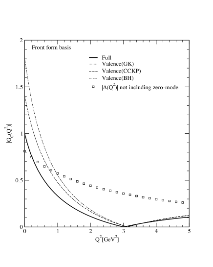
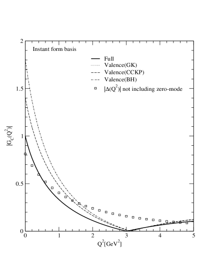
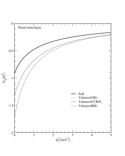
In Fig. 2, we show the charge form factor $|G_{C}(Q^{2})|$ obtained from the light-front (left) and the instant-form (right) spin bases. The full solutions(thick solid line) are obtained from three different prescriptions [2, 3, 4] given by Eqs. (35)-(41) for the light-front basis and Eqs. (A1)-(A6) for the instant-form basis, respectively, and they all turn out to give exactly the same result as the covariant one as they should be. The slope of the full solution gives the charge radius of the bound-state as defined in Eq.(94) and we obtained $\langle r_{C}^{2}\rangle=7.63$ GeV^-2 with the parameter set we used. More detailed discussions on the charge, magnetic and quadrupole radii can be found in subsection IV B 6. In the $q^{+}=0$ frame, the full solutions can be decomposed into the valence contribution and the zero-mode contribution since the nonvalence diagram reduces in the limit $q^{+}\to 0$ to the zero mode. To estimate it, we plot the valence contribution for each prescription, i.e. the dotted line for GK [2], long-dashed line for CCKP [3], and dot-dashed line for BH [4], respectively. The normalization constant $g$ is fixed by requiring the full solution to be normalized to $G_{C}(0)=1$. As one can see in Fig.2, the two results for the valence contributions obtained from the light-front and the instant-form bases exactly coincide with each other. However, only the GK prescription is immune to the zero-mode contribution for both helicity bases. The dotted curve cannot be seen because it is on top of the solid curve. Other prescriptions, CCKP and BH, receive large amounts of zero-mode contributions (i.e. the difference between the full solution and the valence one). As we discussed earlier, the GK prescription does not involve the $G^{+}_{00}$ component which is the only source of the zero-mode for the light-front helicity basis and the zero-modes from the $G^{+}_{xx}$ and $\eta G^{+}_{zz}$ terms in Eq. (A1) for the instant-form basis cancel each other(See Eq. (A11).). We also show the angular condition(small squares) given by Eq. (34) without including the zero-mode contributions. If we include the zero-mode contributions, then it is of course exactly zero.

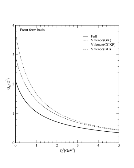
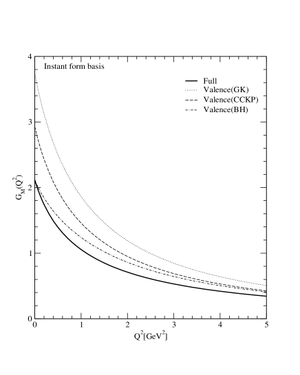
The situation is rather different for the calculation of the magnetic form factor $G_{M}$ as shown in Fig. 3. For the full solution, the two (LF and IF helicity bases) results are again exactly the same as they should be. The magnetic moment (in units of $e/2m$) and its radius given by Eq.(94) are obtained as $\mu_{1}=2.1$ and $\langle r_{M}^{2}\rangle=9.73$ GeV^-2 (See also subsection IV B 6.), respectively. However, the valence (or for that matter the zero-mode) contributions to the full solution are quite different depending on the helicity bases. For the light-front helicity basis, the GK prescription is again immune to the zero-mode and the dotted curve is exactly on top of the solid curve. Also, the other prescriptions, CCKP and BH, receive large amounts of the zero-mode contributions as in the case of the $G_{C}$ calculation. However, for the instant form spin basis used in [8], not only the CCKP and BH prescriptions but also the GK prescription are affected by the zero-mode, because the zero-mode terms $-G^{+}_{zz}$ and $G^{+}_{zx}/\sqrt{\eta}$ in Eq. (A1) do not cancel each other (See Eq. (A11).) but rather add up.

We show in Fig. 4 the quadrupole form factor $G_{Q}(Q^{2})$ obtained from the light-front (left) and the instant-form (right) helicity bases. The quadrupole moments (in units of $e/m^{2}$) and the corresponding radius given by Eq.(94) are obtained as $Q_{1}=0.91$ and $\langle r^{2}_{Q}\rangle=12.6$ GeV^-2 (See also subsection IV B 6.), respectively. As in the case of $G_{C}(Q^{2})$, the two (LF and IF helicity bases) results coincide and the dotted curves are exactly on top of the solid curves because of the absence of the zero-mode in the GK prescription.

The decay constant (See Eqs.(62) and (89).) using the same parameters yields the result $f_{v}=133.7$ MeV, while the experimental data $f_{\rho^{0}}=152.8\pm 3.6$ MeV and $f_{\rho^{\pm}}=147.3\pm 0.7$ MeV are obtained from the width $\Gamma(\rho\rightarrow e^{+}e^{-})$ and the branching ratio $Br(\tau\to\rho\nu_{\tau})=(25.02\pm 0.16)\%$ [21], respectively.

B Light-front valence parts

We checked that in all reference frames the sum of the valence and nonvalence contributions to the form factors is equal to the covariant result. Therefore henceforth we plot the valence contributions only. The valence parts will in general depend on the polar angle $\theta$ in BRT and TRF, but are independent of the azimuthal angle $\phi$ in all three reference frames(DYW,BRT,TRF). We used the latter property as a check of the accuracy of our codes.

Using Eq. (1) for the matrix elements and the kinematics specified in Eqs. (25) and (28) for BRT and TRF, respectively, one finds that the coefficients $b_{i}$ and $c_{i}$, $i=1,2,3$, vanish for $\theta=0$. Therefore we illustrate the angular dependence of the valence parts in BRT and TRF by giving them for the small but nonvanishing value $\theta=\pi/20$. On the other hand $\theta=\pi/2$ is singled out for the BRT frame, so we chose for a larger value of $\theta$ the value $9\pi/20$. There is a symmetry about $\theta=\pi/2$, so the amplitudes for $\pi/2\leq\theta\leq\pi$ don’t contain any additional information.

Eventually we plot the momentum dependence of the valence parts of the form factors and of the violation of the angular conditions for two values of the polar angle $\theta$. We see that in all reference frames and for all angles the angular condition $\Delta_{\rm bd}$ diverges for $Q^{2}\to 0$. This is due to the fact that the coefficient $d_{2}$ of $F_{2}$ in the matrix element $G_{d}$ (See Eq. (13).) vanishes for $Q^{2}=0$. For that reason there is a finite contribution of the nonvalence part or zero mode to the charge form factor even in the limit $Q^{2}\to 0$, which shows up in all $d$ variants of the physical form factors. For finite values of $Q^{2}$ an accidental singularity in $\Delta_{\rm bd}$ may occur. To follow that up we plot the angular variation of the angular conditions for two values of the momentum transfer $Q^{2}$. We can also explain the occurrence of these singularities as due to the vanishing of the coefficient $d_{2}$ of $F_{2}$ in the matrix element $G_{d}$.

1 Drell-Yan-West kinematics

In the DYW reference frame there is no dependence on $\theta$. The dependence on $\phi$ amounts to simple phase factors, $e^{\pm i\phi}$ for $G_{b}$ and $G_{c}$, and $e^{2i\phi}$ for $G_{e}$. In Figs. 5 and 6, the results for the valence parts of the invariant form factors $F_{1}$, $F_{2}$, and $F_{3}$ and the physical ones $G_{C}$, $G_{M}$ and $G_{Q}$ are shown. $F_{1}(0)$ is normalized to 1, which is not affected by the zero mode. For the same reason $G^{b}_{C}(0)=G^{c}_{C}(0)=1$. However, $G^{d}_{C}(0)\neq 1$ and for positive $Q^{2}$ $G^{d}_{C}$ deviates from the correct one by the zero-mode contribution to $F^{d}_{2}$. It is clear that the zero mode is very important if one does choose the $F^{d}_{2}$-prescription. Neither of the $F^{b}_{2}$- or $F^{c}_{2}$-prescription contains the zero mode. As mentioned before, they correspond to the GK-prescription in the DYW-frame for $\phi=0$.

2 Breit frame kinematics

Our convention for the BRT frame entails both $\theta$- and $\phi$-dependences of the matrix elements. The latter being trivial, we fixed $\phi=0$ in all our calculations, after checking that indeed the form factors are independent of this angle. For $\theta=\pi/2$ the BRT frame and the DYW frame can be connected by a kinematical transformation, so the results for the form factors become identical. (See the discussion in [6].) We chose two values for the angle $\theta$, slightly different from $0$ and $\pi/2$ to illustrate the angular dependence of the valence parts of the form factors. The results shown in Figs.7-10 are for $\theta=\pi/20$ and $\theta=9\pi/20$. As shown in Fig.7, it is immediately clear that only $F_{1}$ and $F_{3}$ are rather insensitive to the choice of the polar angle, but the three prescriptions for $F_{2}$ are dramatically changing with $\theta$ going from a small value to one near $\pi/2$. This strong angle-dependence is found also in the physical form factors shown in Figs.8-10, although the $b$- and $c$-variants are much less changed than the $d$-variant. In all cases the charge form factor shows the least angular variation.

3 Target-rest-frame kinematics

The results shown in Figs.11-14 are again for $\theta=\pi/20$ and $\theta=9\pi/20$. Everything we said for the results obtained in the Breit frame can be repeated for the target-rest frame. In Figs.12-14, we see for the $b$- and $c$-variants similar angular dependences, but for the $d$-variant the variation with $\theta$ is even more dramatic than in the Breit frame. The results in Fig.14 for $\theta=9\pi/20$ hint at a singular behaviour of the $d$-variant that is explained by the fact that for some combinations of $Q^{2}$ and $\theta$ the coefficient $d_{2}$ vanishes. We discuss more details of the situation below in Section IV B 5.

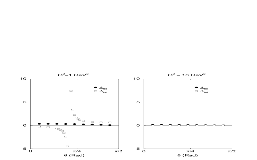
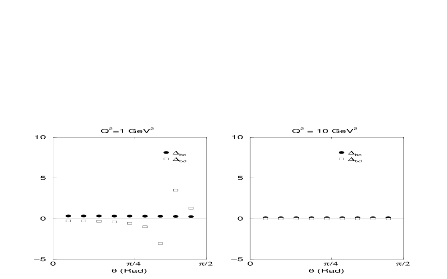
4 Angular condition

In the next plots of Figs.15-17, we show the two angular conditions for a somewhat longer $Q^{2}$ interval, up till 10 GeV². In the case of the Breit (Fig.16) and target-rest(Fig.17) frames we plot the differences $\Delta_{bc}=F^{b}_{2}-F^{c}_{2}$ and $\Delta_{bd}=F^{b}_{2}-F^{d}_{2}$ for four angles $\theta=\pi/8,\,\pi/4,\,3\pi/8,\pi/2$. For the DYW frame(Fig.15) $\Delta_{bc}=0$, so in the plot $\Delta_{bc}$ coincides with the $Q^{2}$-axis.

In the Breit frame the angular conditions do depend on $\theta$ and we show their behaviour for the same angles as in Sec. IV B 2. The angular condition that was trivially fulfilled in the DYW frame turns out to be only weakly violated in the Breit frame. The other one however, $\Delta_{bd}$ is strongly violated for small values of $Q^{2}$. It demonstrates clearly the importance of including the nonvalence parts in a calculation of the matrix elements of the current. For large values of $Q^{2}$ it tends very quickly to zero, corroborating the expectation that in perturbative QCD one may ignore largely the nonvalence parts for sufficiently high momentum tranfers.

Again, the discussion of the behaviour of the angular conditions in the target-rest frame can be very similar to the one for the Breit frame, so we shall not repeat it. We only mention that the overall behaviour is similar in these two cases, but the details differ. In particular, in the following subsection IV B 5 we consider two $Q^{2}$ values ($Q^{2}=1.0$ GeV² and $10.0$ GeV²) and find that the singularity in $\Delta_{bd}$ occurs in the Breit frame for $\theta$ close to $\pi/4$ while in the target-rest frame it shows up for $\theta$ close to $3\pi/8$.

5 Singular behavior

Figure 14 shows that $G^{d}_{C}$ starts to drop significantly when $Q^{2}$ is near to 4 GeV². Such a behavior can be understood from the dependence of the coefficient $d_{2}$ occurring in Eqs. (13) and (14), on the momentum transfer $Q$ and the angle $\theta$. It appears that both in the BRT frame and the TRF this coefficient may vanish for a particular combination of $Q^{2}$ and $\theta$.

The singularity of $\Delta_{bd}$ in the Breit frame is illustrated in Fig. 18. We see that it occurs for $Q^{2}=1.0$ GeV² close to $\theta=\pi/4$. The other angular condition remains flat in $\theta$ and the same is true for both conditions for $Q^{2}=10.0$ GeV². A similar picture is found in Fig. 19 for the target-rest frame, only the position of the singularity being different.

We can understand this behaviour very easily if we consider the expressions for $d_{2}$, that can be derived in a straightforward way from the kinematics and the expressions for the polarization vectors inserted in Eq. (1). We find

$$d^{\rm BRT}_{2}=\frac{\surd 2\beta mQ^{2}[1-\beta^{2}+(1+\beta^{2})\cos 2\theta]}{4\beta^{2}m^{2}-Q^{2}\cos^{2}\theta}$$ (90)

for the Breit frame and

$$d^{TRF}_{2}=\frac{(2m+\kappa+\beta Q\cos\theta)(\kappa^{2}+2\beta\kappa Q\cos\theta+\beta^{2}Q^{2}\cos 2\theta)}{2\surd 2m(m+\kappa+\beta Q\cos\theta)}$$ (91)

for the target-rest frame.

Solving the equation $d_{2}=0$ for $Q^{2}=1.0$ GeV², we find for BRT $\theta=0.698=0.222\pi$ and for TRF $\theta=1.181=0.376\pi$. These angles coincide with the positions of singularities shown in Figs.18 and 19. Also, we note that for $\theta=\frac{\pi}{8}$ in the BRT frame there exists a singularity at $Q^{2}=8m^{2}/(\sqrt{2}-1)\approx 11.45$ GeV² which is not shown in Fig.18 due to the restricted interval of $Q^{2}$ only up to $10$ GeV². However, except the tiny region near this singularity position, the angular condition is very well satisfied at the larger $Q^{2}$ region.

6 Charge, Magnetic and Quadrupole Radii

From the slope of physical form factors for $Q^{2}\to 0$, the corresponding radii ($\langle r^{2}_{C}\rangle,\langle r^{2}_{M}\rangle,\langle r^{2}_{Q}\rangle$) can be defined as

$$G_{C}(Q^{2}) \sim G_{C}(0)\left[1-\frac{1}{6}\langle r^{2}_{C}\rangle Q^{2}\right],$$ (92)

$$G_{M}(Q^{2}) \sim G_{M}(0)\left[1-\frac{1}{10}\langle r^{2}_{M}\rangle Q^{2}\right],$$ (93)

$$G_{Q}(Q^{2}) \sim G_{Q}(0)\left[1-\frac{1}{14}\langle r^{2}_{Q}\rangle Q^{2}\right].$$ (94)

When one considers only the valence parts of charge, magnetic and quadrupole form factors, one should be careful in obtaining the corresponding radii given by Eq.(94) because some of them exhibit singular behaviors as $Q^{2}\to 0$. In order to determine the radii, one may in general try to take the limit $(G(Q^{2})-G(0))/Q^{2}$ as $Q^{2}\to 0$. In practice, however, this gives a rather unreliable value as for very small values of $Q^{2}$ the calculations may have numerical noise that is amplified by taking the difference of two almost equal numbers and dividing the result by the small number $Q^{2}$. A more stable procedure is to make a linear fit to the form factors in a domain close to $Q^{2}=0$. We have chosen the interval $0.01\leq Q^{2}\leq 0.1$ and took ten equidistant values for $Q^{2}$. In order to check whether it makes sense to fit the form factors to a linear function of $Q^{2}$ in this domain, we plotted the form factors as shown in Figs.20-26 and also checked the quality of the fit.

It turned out that only $G_{M}$ and $G_{Q}$ in the $d$-variants could not be fitted with a straight line. The reason is that in these variants the influence of the zero mode is very big and only including the zero mode or the nonvalence part can correct the nonlinear behaviour. Because of this reason, we do not show the $d$-variant valence results for $G_{M}$ and $G_{Q}$ which are anyway out of scale in Figs.20,23 and 26. However, in the case that includes the nonvalence part as shown in Figs.21-23 (total in BRT) and Figs.24-26 (total in TRF), all values obtained for the radii do agree. The same is true for the case where the zero mode does not occur as shown in Fig.20 ($b$- and $c$-variants in DYW). An indication of the accuracy of the results is obtained if one includes the values at $Q^{2}=0$ in the fit. Then the radii do not change by more than 1.5%. If one would try do determine these quantities by fitting the form factors in a much smaller interval, say $.001\leq Q^{2}\leq 0.01$ in order to improve the linear approximation mathematically, then the numerical noise will have a stronger influence. So there is a trade off between truncation error in the series expansion of the Bessel function and numerical noise. We are satisfied with an overall numerical error of the order of 1%. In Table I, we summarize the numerical results of radii. For the $d$-variants, both $G_{M}$ and $G_{Q}$ diverges for $Q^{2}\to 0$ as discussed above and an entry ‘div.’ is given for those cases in this Table. The numerical estimates for the radii in these divergent cases, which do not include $Q^{2}=0$, give indeed values of the order of a hundred GeV^-2.

TABLE I.: Squared radii in GeV^-2 for the different reference frames and variants.

Ref. frame, variant	$G_{C}$	$G_{M}$	$G_{Q}$
DYW, $G^{b}$ and $G^{c}$	7.63	9.73	12.6
DYW, $G^{d}$	9.56	div.	div.
	$\theta=\pi/20$
BRT, tot	7.63	9.73	12.6
BRT, $G^{b}$, val	14.3	27.6	50.4
BRT, $G^{c}$, val	14.7	18.3	19.4
BRT, $G^{d}$, val	13.9	div.	div.
	$\theta=9\pi/20$
BRT, tot	7.63	9.73	12.6
BRT, $G^{b}$, val	8.42	12.0	17.7
BRT, $G^{c}$, val	8.48	10.7	13.6
BRT, $G^{d}$, val	10.0	div.	div.
	$\theta=\pi/20$
TRF, tot	7.63	9.73	12.6
TRF, $G^{b}$, val	14.3	27.7	50.6
TRF, $G^{c}$, val	14.8	18.3	19.5
TRF, $G^{d}$, val	14.1	div.	div.
	$\theta=9\pi/20$
TRF, tot	7.63	9.73	12.6
TRF, $G^{b}$, val	9.84	15.9	26.2
TRF, $G^{c}$, val	9.98	12.5	15.2
TRF, $G^{d}$, val	15.5	div.	div.

V Conclusion

In this work, we made a taxonomical analysis of spin-1 form factors with respect to several different prescriptions (GK,CCKP,BH), polarization vector choices (LF,IF), and reference frames (DYW,BRT,TRF). We used the $J^{+}$ current for all of our analysis.

In the $q^{+}=0$ frame, we looked at both LF and IF polarization vectors and made a comparative analysis on the three prescriptions (GK,CCKP,BH) in relating the matrix elements to the physical form factors. In the light-front gauge, $A^{+}=0$, the light-front helicity basis is the set of eigenvectors of the light-front helicity operator. However, the instant-form polarization vectors have been also used in the literature. We find that the zero-mode contamination occurs minimally in the light-front gauge because only the helicity zero to zero amplitude, i.e. $G^{+}_{00}$, gets a zero-mode contribution, but all others ($G^{+}_{++},\,G^{+}_{+0},\,G^{+}_{+-}$) are immune from the zero-mode in the light-front basis. Thus, one can find a prescription which doesn’t involve the zero mode contribution at all. Indeed, the GK prescription which doesn’t use $G^{+}_{00}$ has precisely this property. Consequently, the computation of only the valence contributions to the form factors using the GK prescription yields results which coincide exactly with the full results of the form factors as we have shown in Figs.2-4. These full results can be obtained by the other prescriptions, CCKP and BH, only if the zero-mode contributions are added to the valence contributions. We have also computed the form factors using a manifestly covariant Feynman method and explicitly shown that the full results of the light-front calculations are fully in agreement with the covariant one no matter what prescriptions we use. Although the full results are also independent of the choice of the polarization vectors, we find that the nice feature of the GK prescription described above is lost in the instant-form basis. As shown in Fig.3, the valence contribution to the magnetic form factor ($G_{M}(Q^{2})$) computed in the instant-form basis substantially differs from the full result even if the GK prescription is used. This is due to the fact that a larger number of matrix elements are contaminated by the zero-mode in the instant-form basis and in the particular case of $G_{M}(Q^{2})$ the terms affected by the zero-mode such as $-G^{+}_{zz}$ and $G^{+}_{zx}/\sqrt{\eta}$ in Eq. (A1) do not cancel each other (See Eq. (A11).) but rather add up. We thus conclude that the GK prescription in the light-front basis is certainly advantageous for model calculation involving only the valence contributions to the spin-1 form factors.

We have also analyzed the frame dependence of the valence contribution to the physical form factors and the angular conditions using the light-front polarization vectors. Since the three presciptions discussed above are defined only in the $q^{+}=0$ frame, we use the prescriptions $b$, $c$, and $d$ defined in Section II to work in a general frame. In DYW frame, our $c$ prescription corresponds to the GK prescription and the results on the form factors from our $b$ prescription coincide with those from the $c$ or GK prescription. Also, some combinations of the $c$ and $d$ prescriptions correspond to the CCKP and BH prescriptions depending on the coefficients of the combinations. Again, only the $d$ prescription involves the zero-mode and the valence result from the $d$ prescription differs from the results of the $b$ and $c$ prescriptions that coincide each other exactly as shown in Figs. 5 and 6. The results in the Breit frame reproduce the DYW results if $\theta=\pi/2$, since they can be transformed into each other by purely kinematic operators in LFD. If $\theta\neq\pi/2$, however, the results are quite different from the DYW results. As shown in Figs. 7-10 more drastic differences in the results among the $b$, $c$, and $d$ prescriptions are found at $\theta=\pi/20$ than at $\theta=9\pi/20$. Similar observations can be made also for the TRF. However, the kinematic equivalence to DWY obtains only at a special angle $\theta=\theta_{0}$ (See Ref. [19].) which depends on $Q^{2}$. Thus, it is rather difficult to see the similarity of the results of TRF and DYW. Although the angular condition $\Delta_{bc}$ is rather well satisfied, the usual angular condition $\Delta_{bd}$ is severely broken in the small $Q^{2}$ region. Singularities associated with those violations are visible in our figures(See e.g. Figs.18 and 19.).

Nevertheless, both angular conditions $\Delta_{bc}$ and $\Delta_{bd}$ are well satisfied in the region $Q^{2}$ above a few GeV² except the tiny region near the singularity position discussed in Section IV B 5. and thus the results from all the prescriptions become consistent with each other. Thus, one may conclude that the zero-mode contributions are highly suppressed in the high $Q^{2}$ region and the results are consistent with the perturbative QCD predictions. This may justify the use of the BH prescription in the analysis of high $Q^{2}$ form factors. For the low and intermediate $Q^{2}$ regions, however, the zero-mode contributions are very important and the GK prescription with the light-front polarization vectors in the DYW frame is certainly desirable for the form factor analyses. An application of this observation to a more realistic model calculation is under consideration.

A Form factors in the instant-form basis

Using the instant-form linear polarization vectors ($h,h^{\prime}=x,y,z$), the form factors corresponding to Eqs. (35)-(41) in the light-front polarization vectors are given by [8]

$$G_{C}^{\rm GK} = \frac{1}{2p^{+}}\biggl{[}\frac{1}{3}G^{+}_{xx}+\frac{(2-\eta)}{3}G^{+}_{yy}+\frac{\eta}{3}G^{+}_{zz}\biggr{]},$$ (A1)

$$G_{M}^{\rm GK} = -\frac{1}{2p^{+}}\biggl{[}G^{+}_{yy}-G^{+}_{zz}+\frac{G^{+}_{zx}}{\sqrt{\eta}}\biggr{]},$$ (A2)

$$G_{Q}^{\rm GK} = \frac{1}{2p^{+}}\biggl{[}\frac{1}{2\eta}G^{+}_{xx}-\frac{(1+\eta)}{2\eta}G^{+}_{yy}+\frac{1}{2}G^{+}_{zz}\biggr{]},$$ (A3)

$$G_{C}^{\rm CCKP} = \frac{1}{2p^{+}}\biggl{[}\frac{1}{3}G^{+}_{xx}+\frac{1}{6}G^{+}_{yy}+\frac{1}{2}G^{+}_{zz}\biggr{]},$$ (A4)

$$G_{M}^{\rm CCKP} = -\frac{1}{2p^{+}}\frac{G^{+}_{zx}}{\sqrt{\eta}},\;\;G_{Q}^{\rm CCKP}=\frac{1}{2p^{+}}\frac{(G^{+}_{xx}-G^{+}_{yy})}{2\eta},$$ (A5)

and

$$G_{C}^{\rm BH} = \frac{1}{2p^{+}(1+2\eta)}\biggl{[}\frac{(1+2\eta)}{3}G^{+}_{xx}+\frac{(2\eta-1)}{3}G^{+}_{yy}+\frac{(3+2\eta)}{3}G^{+}_{zz}\biggr{]},$$ (A6)

$$G_{M}^{\rm BH} = \frac{-1}{2p^{+}(1+2\eta)}\biggl{[}\frac{(1+2\eta)}{\sqrt{\eta}}G^{+}_{zx}-G^{+}_{yy}+G^{+}_{zz}\biggr{]},$$ (A7)

$$G_{Q}^{\rm BH} = \frac{1}{2p^{+}(1+2\eta)}\biggl{[}\frac{(1+2\eta)}{2\eta}G^{+}_{xx}-\frac{(1+\eta)}{2\eta}G^{+}_{yy}-\frac{1}{2}G^{+}_{zz}\biggr{]},$$ (A8)

where we redefine the definition of the form factors $G_{0},G_{1}$, and $G_{2}$ in Ref. [8] in terms of $G_{C},G_{M}$, and $G_{Q}$ according to footnote 1. In order to calculate the form factors of a spin-1 particle in this instant-form bases, the authors of Ref. [7, 8] used the reference frame specified in our Eq. (29). However, they use different (i.e. non LF gauge) polarization vectors in the initial($\epsilon$) and final($\epsilon^{\prime}$) states that are given by

$$\epsilon^{\mu}_{x} = (-\sqrt{\eta},\sqrt{1+\eta},0,0),\;\epsilon^{\mu}_{y}=(0,0,1,0),\;\epsilon^{\mu}_{z}=(0,0,0,1),$$ (A9)

and

$$\epsilon^{\prime\mu}_{x} = (\sqrt{\eta},\sqrt{1+\eta},0,0),\;\epsilon^{\prime\mu}_{y}=\epsilon^{\mu}_{y},\;\epsilon^{\prime\mu}_{z}=\epsilon^{\mu}_{z}.$$ (A10)

(Here we use the component convention $p^{\mu}=(p^{0},p^{1},p^{2},p^{3})$ etc.) Even though these polarization vectors satisfy the correct orthonormality and closure relations as well as the conditions $\epsilon\cdot p=\epsilon^{\prime}\cdot p^{\prime}=0$, they cannot be obtained in the LF gauge.

Proceeding to calculate the trace terms $S^{+}_{xx},S^{+}_{yy},S^{+}_{zz}$ and $S^{+}_{zx}$ using Eqs. (A9), and (A10), we obtain

$$S^{+}_{xx} = \underline{-4k^{-}\eta\biggl{[}m^{2}_{q}+\vec{k}^{2}_{\perp}-\eta m^{2}\biggr{]}}+4k^{-}p^{+}(p^{+}-k^{+})(1-x-\eta-\eta x)$$ (A11)

$$+ 4p^{+}\biggl{[}4(x+\eta x-1)k^{2}_{x}-\eta(1+\eta)x^{3}m^{2}-(x+3\eta x-2)(m^{2}_{q}+\vec{k}^{2}_{\perp})\biggr{]},$$ (A12)

$$S^{+}_{yy} = 4k^{-}(k^{+}-p^{+})^{2}-4p^{+}\biggl{[}4(1-x)k^{2}_{y}+\eta xm^{2}-(2-x)(m^{2}_{q}+\vec{k}^{2}_{\perp})\biggr{]},$$ (A13)

$$S^{+}_{zz} = \underline{4k^{-}\biggl{[}m^{2}_{q}+\vec{k}^{2}_{\perp}-\eta m^{2}\biggr{]}}+4(1-x)p^{+}\biggl{[}x(1-x)(1+\eta)m^{2}+2(m^{2}_{q}+\vec{k}^{2}_{\perp})\biggr{]},$$ (A14)

$$S^{+}_{zx} = \underline{-4k^{-}\sqrt{\eta}\biggl{[}m^{2}_{q}+\vec{k}^{2}_{\perp}-\eta m^{2}\biggr{]}}+4\sqrt{\eta}k^{-}p^{+}(k^{+}-p^{+})$$ (A15)

$$+ 4\sqrt{\eta}p^{+}\biggl{[}2k^{2}_{x}-x^{2}(1-x)(1+\eta)m^{2}-2(m^{2}_{q}+\vec{k}^{2}_{\perp})\biggr{]},$$ (A16)

where $\surd 2p^{+}=p^{0}=m\sqrt{1+\eta}$ and we omit the terms of odd power in $\vec{k}_{\perp}$ since they do not contribute to the integral. Note also that we do not separate the on-shell propagating part from the instantaneous one in this instant-form calculation. As we discussed, only the underlined terms in $S^{+}_{xx},S^{+}_{zz}$ and $S^{+}_{zx}$ contribute to the zero-mode part and the $S^{+}_{yy}$ component is immune to the zero-mode contributions.

B Derivation of the zero-mode

In this appendix, we derive Eq. (85) in detail. Performing the $k^{-}$-integration in Eq. (85), the residue at the pole $k^{-}=p^{\prime+}+[(\vec{k}_{\perp}-\vec{p^{\prime}}_{\perp})^{2}+\Lambda^{2}]/2(k^{+}-p^{\prime+})$ gives

$$G^{+{\rm z.m.}}_{h^{\prime}h} = i\int\frac{d^{4}k}{(2\pi)^{4}}\frac{k^{-}}{D_{k}D_{\Lambda}D^{\prime}_{\Lambda}}$$ (B1)

$$= \frac{i}{(2\pi)^{4}}\int\frac{dk^{+}dk^{-}d^{2}\vec{k}_{\perp}}{2k^{+}2(k^{+}-p^{+})2(k^{+}-p^{\prime+})}$$ (B3)

$$\times\frac{k^{-}}{\biggl{[}k^{-}-\frac{\vec{k}^{2}_{\perp}+m^{2}_{q}-i\varepsilon}{2k^{+}}\biggr{]}\biggl{[}k^{-}-p^{-}-\frac{(\vec{k}_{\perp}-\vec{p}_{\perp})^{2}+\Lambda^{2}-i\varepsilon}{2(k^{+}-p^{+})}\biggr{]}\biggl{[}k^{-}-p^{\prime-}-\frac{(\vec{k}_{\perp}-\vec{p^{\prime}}_{\perp})^{2}+\Lambda^{2}-i\varepsilon}{2(k^{+}-p^{\prime+})}\biggr{]}},$$

$$= -\frac{1}{(2\pi)^{3}}\int^{p^{\prime+}}_{p^{+}}\frac{dk^{+}d^{2}\vec{k}_{\perp}}{2k^{+}2(k^{+}-p^{+})2(k^{+}-p^{\prime+})}$$ (B5)

$$\times\frac{k^{-}}{\biggl{[}p^{\prime-}+\frac{(\vec{k}_{\perp}-\vec{p^{\prime}}_{\perp})^{2}+\Lambda^{2}}{2(k^{+}-p^{\prime+})}-\frac{\vec{k}^{2}_{\perp}+m^{2}_{q}}{2k^{+}}\biggr{]}\biggl{[}p^{\prime-}-p^{-}+\frac{(\vec{k}_{\perp}-\vec{p^{\prime}}_{\perp})^{2}+\Lambda^{2}}{2(k^{+}-p^{\prime+})}-\frac{(\vec{k}_{\perp}-\vec{p}_{\perp})^{2}+\Lambda^{2}}{2(k^{+}-p^{+})}\biggr{]}},$$

$$= -\frac{1}{2(2\pi)^{3}}\int^{p^{\prime+}}_{p^{+}}dk^{+}d^{2}\vec{k}_{\perp}p^{+}(p^{\prime+})^{2}(k^{+}-p^{\prime+})k^{-}$$ (B9)

$$\times\frac{1}{\biggl{\{}k^{+}(k^{+}-p^{\prime+})(m^{2}+\vec{p^{\prime}}^{2}_{\perp})+p^{\prime+}k^{+}[(\vec{k}_{\perp}-\vec{p^{\prime}}_{\perp})^{2}+\Lambda^{2}]-p^{\prime+}(k^{+}-p^{\prime+})(\vec{k}^{2}_{\perp}+m^{2}_{q})\biggr{\}}}$$

$$\times\frac{1}{\biggl{\{}p^{+}(k^{+}-p^{+})(k^{+}-p^{\prime+})(m^{2}+\vec{p^{\prime}}^{2}_{\perp})-p^{\prime+}(k^{+}-p^{+})(k^{+}-p^{\prime+})(m^{2}+\vec{p}^{2}_{\perp})}$$

$$\hskip 14.22636pt+p^{+}p^{\prime+}(k^{+}-p^{+})[(\vec{k}_{\perp}-\vec{p^{\prime}}_{\perp})^{2}+\Lambda^{2}]-p^{+}p^{\prime+}(k^{+}-p^{\prime+})[(\vec{k}_{\perp}-\vec{p}_{\perp})^{2}+\Lambda^{2}]\biggr{\}}$$

$$= -\frac{1}{2(2\pi)^{3}}\int^{p^{\prime+}}_{p^{+}}dk^{+}d^{2}\vec{k}_{\perp}\;p^{+}(p^{\prime+})^{2}(k^{+}-p^{\prime+})k^{-}$$ (B13)

$$\times\frac{1}{\biggl{\{}k^{+}(k^{+}-p^{\prime+})(m^{2}+\vec{p}^{2}_{\perp})+p^{\prime+}k^{+}[(\vec{k}_{\perp}-\vec{p^{\prime}}_{\perp})^{2}+\Lambda^{2}]-p^{\prime+}(k^{+}-p^{\prime+})(\vec{k}^{2}_{\perp}+m^{2}_{q})\biggr{\}}}$$

$$\times\frac{1}{\biggl{\{}(-q^{+})(k^{+}-p^{+})(k^{+}-p^{\prime+})(m^{2}+\vec{p}^{2}_{\perp})+p^{+}p^{\prime+}(k^{+}-p^{+})[(\vec{k}_{\perp}-\vec{p^{\prime}}_{\perp})^{2}+\Lambda^{2}]}$$

$$\hskip 14.22636pt-p^{+}p^{\prime+}(k^{+}-p^{\prime+})[(\vec{k}_{\perp}-\vec{p}_{\perp})^{2}+\Lambda^{2}]\biggr{\}},$$

where we use $\vec{p}^{2}_{\perp}=\vec{p^{\prime}}^{2}_{\perp}$ and $q^{+}=p^{\prime+}-p^{+}$ in the derivation of the last term in Eq. (B1). Writing $q^{+}=\delta p^{+}$ and $p^{\prime+}=(1+\delta)p^{+}$, $\delta\to 0$ at the end, we obtain

$$G^{+{\rm z.m.}}_{h^{\prime}h} = -\frac{1}{2(2\pi)^{3}}{\rm lim}_{\delta\to 0}\int^{1+\delta}_{1}dx\;d^{2}\vec{k}_{\perp}(x-1-\delta)(1+\delta)^{2}\biggl{[}\frac{m^{2}+\vec{p^{\prime}}^{2}_{\perp}}{(1+\delta)p^{+}}+\frac{(\vec{k}_{\perp}-\vec{p^{\prime}}_{\perp})^{2}+\Lambda^{2}}{(x-1-\delta)p^{+}}\biggr{]}$$ (B17)

$$\times\frac{1}{\biggl{\{}x(x-1-\delta)(m^{2}+\vec{p}^{2}_{\perp})+(1+\delta)x[(\vec{k}_{\perp}-\vec{p^{\prime}}_{\perp})^{2}+\Lambda^{2}]-(1+\delta)(x-1-\delta)(\vec{k}^{2}_{\perp}+m^{2}_{q})\biggr{\}}}$$

$$\times\frac{1}{\biggl{\{}-\delta(x-1)(x-1-\delta)(m^{2}+\vec{p}^{2}_{\perp})+(1+\delta)(x-1)[(\vec{k}_{\perp}-\vec{p^{\prime}}_{\perp})^{2}+\Lambda^{2}]}$$

$$\hskip 14.22636pt-(1+\delta)(x-1-\delta)[(\vec{k}_{\perp}-\vec{p}_{\perp})^{2}+\Lambda^{2}]\biggr{\}}.$$

If we write $x=1+\delta\,y$ and $dx=\delta\,dy$, then the integral over $y$ runs from 0 to 1 as $x$ runs from 1 to $1+\delta$. Therefore, we get

$$G^{+{\rm z.m.}}_{h^{\prime}h} = -\frac{1}{2p^{+}(2\pi)^{3}}\int^{1}_{0}dy\;d^{2}\vec{k}_{\perp}\frac{1}{\biggl{\{}y[(\vec{k}_{\perp}-\vec{p^{\prime}}_{\perp})^{2}+\Lambda^{2}]+(1-y)[(\vec{k}_{\perp}-\vec{p}_{\perp})^{2}+\Lambda^{2}]\biggr{\}}}$$ (B18)

$$= \frac{1}{2p^{+}(2\pi)^{3}}\int\;d^{2}\vec{k}_{\perp}\frac{{\rm ln}\biggl{[}\frac{(\vec{k}_{\perp}-\vec{p^{\prime}}_{\perp})^{2}+\Lambda^{2}}{(\vec{k}_{\perp}-\vec{p}_{\perp})^{2}+\Lambda^{2}}\biggr{]}}{[(\vec{k}_{\perp}-\vec{p}_{\perp})^{2}+\Lambda^{2}]-[(\vec{k}_{\perp}-\vec{p^{\prime}}_{\perp})^{2}+\Lambda^{2}]}.$$ (B19)

FIG. 2.: The charge form factor $|G_{C}(Q^{2})|$ obtained from the light-front (left) and the instant-form (right) spin bases: The thick solid line represents the full (i.e. valence+zero-mode in LF = covariant) solution. The dotted, long-dashed, and dot-dashed lines represent the valence contributions only, where we use the same normalization as for the full solution $G_{C}(0)=1$. The small squares represent the angular condition in Eq. (34) without including the zero-mode contribution.

FIG. 3.: The magnetic form factor $G_{M}(Q^{2})$ obtained from the light-front (left) and the instant form (right) spin bases. The same lines are used as in Fig 2.

FIG. 4.: The quadrupole form factor $G_{Q}(Q^{2})$ obtained from the light-front (left) and the instant form (right) spin bases. The same lines are used as in Fig 2.

FIG. 5.: Invariant form factors $F_{1}$, $F^{b}_{2}$, $F^{c}_{2}$, $F^{d}_{2}$, and $F_{3}$ (left) and physical form factors $G_{C}$, $G_{M}$, and $G_{Q}$ from $F^{b}_{2}$ (right) calculated in the Drell-Yan-West frame. Valence parts only.

FIG. 6.: Physical form factors $G_{C}$, $G_{M}$, and $G_{Q}$ from $F^{c}_{2}$ (left) and $F^{d}_{2}$ (right) calculated in the Drell-Yan-West frame. Valence parts only.

FIG. 7.: Invariant form factors $F_{1}$, $F^{b}_{2}$, $F^{c}_{2}$, $F^{d}_{2}$, and $F_{3}$ for $\theta=\pi/20$ (left) and $\theta=9\pi/20$ (right) calculated in the Breit frame. Valence parts only.

FIG. 8.: Physical form factors $G_{C}$, $G_{M}$, and $G_{Q}$ from $F^{b}_{2}$ calculated in the Breit frame. Left $\theta=\pi/20$, right $\theta=9\pi/20$. Valence parts only.

FIG. 9.: Physical form factors $G_{C}$, $G_{M}$, and $G_{Q}$ from $F^{c}_{2}$ calculated in the Breit frame. Left $\theta=\pi/20$, right $\theta=9\pi/20$. Valence parts only.

FIG. 10.: Physical form factors $G_{C}$, $G_{M}$, and $G_{Q}$ from $F^{d}_{2}$ calculated in the Breit frame. Left $\theta=\pi/20$, right $\theta=9\pi/20$. Valence parts only.

FIG. 11.: Invariant form factors $F_{1}$, $F^{b}_{2}$, $F^{c}_{2}$, $F^{d}_{2}$, and $F_{3}$ for $\theta=\pi/20$ (left) and $\theta=9\pi/20$ (right) calculated in the target-rest-frame. Valence parts only.

FIG. 12.: Physical form factors $G_{C}$, $G_{M}$, and $G_{Q}$ from $F^{b}_{2}$ calculated in the target-rest-frame. Version $b$. Left $\theta=\pi/20$, right $\theta=9\pi/20$. Valence parts only.

FIG. 13.: Physical form factors $G_{C}$, $G_{M}$, and $G_{Q}$ from $F^{c}_{2}$ calculated in the target-rest-frame. Left $\theta=\pi/20$, right $\theta=9\pi/20$. Valence parts only.

FIG. 14.: Physical form factors $G_{C}$, $G_{M}$, and $G_{Q}$ from $F^{d}_{2}$ calculated in the target-rest-frame. Left $\theta=\pi/20$, right $\theta=9\pi/20$. Valence parts only.

FIG. 15.: Angular conditions $\Delta_{\rm bc}$ and $\Delta_{\rm bd}$ in the Drell-Yan-West frame.

FIG. 16.: Dependence of the angular conditions $\Delta_{\rm bc}$ and $\Delta_{\rm bd}$ in the Breit frame on $Q^{2}$ for four different angles $\theta$.

FIG. 17.: Dependence of the angular conditions $\Delta_{\rm bc}$ and $\Delta_{\rm bd}$ in the target-rest frame on $Q^{2}$ for four different angles $\theta$. Note the changed scale in the case $\theta=3\pi/8$. The singlularity is clearly visible there.

FIG. 18.: Angular conditions $\Delta_{\rm bc}$ and $\Delta_{\rm bd}$ in the Breit frame for $Q^{2}=1.0$ GeV² and $Q^{2}=10.0$ GeV² for different angles $\theta$.

FIG. 19.: Angular conditions $\Delta_{\rm bc}$ and $\Delta_{\rm bd}$ in the target-rest frame for $Q^{2}=1.0$ GeV² and $Q^{2}=10.0$ GeV² for different angles $\theta$.

FIG. 20.: Valence contributions to physical form factors for small values of $Q^{2}$ in DYW frame. While $b$ and $d$ variants are shown here, the $d$-variant magnetic($G^{d}_{M}$) and quadrupole($G^{d}_{Q}$) form factors are out of scale because they diverge as $Q^{2}\to 0$.

FIG. 21.: Physical form factors for small values of $Q^{2}$. BRT frame, variant $b$.

FIG. 22.: Physical form factors for small values of $Q^{2}$. BRT frame, variant $c$.

FIG. 23.: Physical form factors for small values of $Q^{2}$. BRT frame, variant $d$.

FIG. 24.: Physical form factors for small values of $Q^{2}$. TRF, variant $b$.

FIG. 25.: Physical form factors for small values of $Q^{2}$. TRF, variant $c$.

FIG. 26.: Physical form factors for small values of $Q^{2}$. TRF, variant $d$.

REFERENCES

- [1] B. L. G. Bakker, H.-M. Choi, and C.-R. Ji, Phys. Rev. D 63, 074014 (2001).
- [2] I. L. Grach and L. A. Kondratyuk, Sov. J. Nucl. Phys. 39, 198 (1984).
- [3] P. L. Chung, F. Coester, B. D. Keister and W. N. Polyzou, Phys. Rev. C 37, 2000 (1988).
- [4] S. J. Brodsky and J. R. Hiller, Phys. Rev. D 46, 2141 (1992).
- [5] F. Cardarelli, I. L. Grach, I. M. Narodetskii, G. Salme, and S. Simula, Phys. Lett. B 349, 393 (1995).
- [6] B. L. G. Bakker and C.-R. Ji, Phys. Rev. D 65, 03xxxx (2002) [hep-ph/0109005].
- [7] J.P.B.C. de Melo et al., Nucl. Phys. A 631, 574c (1998); Nucl. Phys. A 660, 219 (1999).
- [8] J.P.B.C. de Melo and T. Frederico, Phys. Rev. C 55, 2043 (1997).
- [9] D. Melikhov and S.Simula, hep-ph/0112044.
- [10] R. G. Arnold, C. E. Carlson and F. Gross, Phys. Rev. C 21, 1426 (1980).
- [11] B. D. Keister, Phys. Rev. D 49, 1500 (1994).
- [12] H.-M. Choi and C.-R. Ji, Nucl. Phys. A 618, 291 (1997).
- [13] L. L. Frankfurt, T. Frederico, and M. Strikman, Phys. Rev. C 48, 2182 (1993).
- [14] S.-J. Chang and T.-M. Yan, Phys. Rev. D 7, 1147 (1973); Phys. Rev. D 7, 1780 (1973).
- [15] M. Burkardt, Nucl. Phys. A 504, 762 (1989).
- [16] S. J. Brodsky and D. S. Hwang, Nucl. Phys. B 543, 239 (1998).
- [17] N. C. J. Schoonderwoerd and B. L. G. Bakker, Phys. Rev. D 57, 4965 (1998); Phys. Rev. D 58, 025013 (1998).
- [18] H.-M. Choi and C.-R. Ji, Phys. Rev. D 58, 071901 (1998).
- [19] B. L. G. Bakker and C.-R. Ji, Phys. Rev. D 62, 074014 (2000).
- [20] W. Jaus, Phys. Rev. D 60, 054026 (1999).
- [21] Particle Data Group, C. Caso et al., Eur. Phys. J. C3, 1 (1998).