Abstract

Recent measurements from the HERMES and SMC collaborations show a remarkably large azimuthal single-spin asymmetries $A_{UL}$ and $A_{UT}$ of the proton in semi-inclusive pion leptoproduction $\gamma^{*}(q)p\to\pi X$. We show that final-state interactions from gluon exchange between the outgoing quark and the target spectator system lead to single-spin asymmetries in deep inelastic lepton-proton scattering at leading twist in perturbative QCD; i.e., the rescattering corrections are not power-law suppressed at large photon virtuality $Q^{2}$ at fixed $x_{bj}$. The existence of such single-spin asymmetries requires a phase difference between two amplitudes coupling the proton target with $J^{z}_{p}=\pm{1\over 2}$ to the same final-state, the same amplitudes which are necessary to produce a nonzero proton anomalous magnetic moment. We show that the exchange of gauge particles between the outgoing quark and the proton spectators produces a Coulomb-like complex phase which depends on the angular momentum $L^{z}$ of the proton’s constituents and is thus distinct for different proton spin amplitudes. The single-spin asymmetry which arises from such final-state interactions does not factorize into a product of distribution function and fragmentation function, and it is not related to the transversity distribution $\delta q(x,Q)$ which correlates transversely polarized quarks with the spin of the transversely polarized target nucleon.

1 Introduction

Single-spin asymmetries in hadronic reactions have been among the most difficult phenomena to understand from basic principles in QCD. The problem has become more acute because of the observations by the HERMES [1] and SMC [2] collaborations of a strong correlation between the target proton spin $\vec{S}_{p}$ and the plane of the produced pion and virtual photon in semi-inclusive deep inelastic lepton scattering $\ell p^{\uparrow}\to\ell^{\prime}\pi X$ at photon virtuality as large as $Q^{2}=6$ GeV². Large azimuthal single-spin asymmetries have also been seen in hadronic reactions such as $pp^{\uparrow}\to\pi X$ [3], where the target antiproton is polarized normal to the pion production plane, and in $pp\to\Lambda^{\uparrow}X$ [4], where the hyperon is polarized normal to the production plane.

In the target rest frame, single-spin correlations correspond to the $T$-odd triple product $i\vec{S}_{p}\cdot\vec{p}_{\pi}\times\vec{q},$ where the phase $i$ is required by time-reversal invariance. The differential cross section thus has an azimuthal asymmetry proportional to $|\vec{p}_{\pi}||\vec{q}|{\rm sin}\theta_{q\pi}{\rm sin}\phi$ where $\phi$ is the angle between the plane containing the photon and pion and the plane containing the photon and proton polarization vector $\vec{S}_{p}.$ In a general frame, the azimuthal asymmetry has the invariant form ${i\over M}\epsilon_{\mu\nu\sigma\tau}P^{\mu}S_{p}^{\nu}p^{\sigma}_{\pi}q^{\tau}$ where the polarization four-vector of the proton satisfies $S_{p}^{2}=-1$ and $S_{p}\cdot P=0.$

In order to produce a correlation involving a transversely-polarized proton, there are two necessary conditions: (1) There must be two proton spin amplitudes
$M[{\gamma^{*}p(J^{z}_{p})\to F}]$ with $J^{z}_{p}=\pm{1\over 2}$ which couple to the same final-state $|F>$; and (2) The two amplitudes must have different, complex phases. The correlation is proportional to ${\rm Im}(M[J^{z}_{p}=+{1\over 2}]^{*}M[J^{z}_{p}=-{1\over 2}])$. The analysis of single-spin asymmetries thus requires an understanding of QCD at the amplitude level, well beyond the standard treatment of hard inclusive reactions based on the factorization of distribution functions and fragmentation functions. Since we need the interference of two amplitudes which have different proton spin $J^{z}_{p}=\pm{1\over 2}$ but couple to the same final-state, the orbital angular momentum of the two proton wavefunctions must differ by $\Delta L^{z}=1.$ The anomalous magnetic moment for the proton is also proportional to the interference of amplitudes $M[{\gamma^{*}p(J^{z}_{p})\to F}]$ with $J^{z}_{p}=\pm{1\over 2}$ which couple to the same final-state $|F>$.

Final-state interactions (FSI) in gauge theory can affect deep inelastic scattering reactions in a profound way, as has been demonstrated recently [5]. The rescattering of the outgoing quark leads to a leading twist contribution to the deep inelastic cross section from diffractive channels $\gamma^{*}p\to q\overline{q}p^{\prime},$ and the interference effects induced by these diffractive channels cause nuclear shadowing. Here we shall show that FSI also provide the required phase needed to produce single-spin asymmetries in deep inelastic scattering.

The dynamics of the constituents in the target can be described by its light-front wavefunctions, $\psi_{n/p}(x_{i},\vec{k}_{\perp i},\lambda_{i}),$ the projections of the hadronic eigenstate on the free color-singlet Fock state $|n>$ at a given light-cone time $\tau=t+z/c.$ The wavefunctions are Lorentz-invariant functions of the relative coordinates $x_{i}=k^{+}_{i}/P^{+}=(k^{0}_{i}+k^{z}_{i})/(P^{0}+P^{z})$ and ${\vec{k}_{\perp i}}$ [with $\sum^{n}_{i=1}x_{i}=1$ and $\sum^{n}_{i=1}{\vec{k}_{\perp i}}={\vec{0}_{\perp}}],$ and they are independent of the bound state’s physical momentum $P^{+}$ and ${\vec{P}_{\perp}}$ [6]. The physical transverse momenta are ${\vec{p}_{\perp i}}=x_{i}{\vec{P}_{\perp}}+{\vec{k}_{\perp i}}.$ The $\lambda_{i}$ label the light-front spin $S^{z}$ projections of the quarks and gluons along the quantization $z$ direction. If a target is stable, its light-front wavefunction must be real. Thus the only source of a nonzero complex phase in leptoproduction in the light-front frame are final-state interactions. The rescattering corrections from final-state exchange of gauge particles produce Coulomb-like complex phases which, however, depend on the proton spin. Thus $M[{\gamma^{*}p(J^{z}_{p}=\pm{1\over 2})\to F}]=|M[{\gamma^{*}p(J^{z}_{p}=\pm{1\over 2})\to F}]|\,e^{i\chi_{\pm}}$. Each of the phases is infrared divergent; however the difference $\Delta\chi=\chi_{+}-\chi_{-}$ is infrared finite and nonzero. The resulting single-spin asymmetry is then proportional to ${\rm sin}\Delta\chi.$

2 A Model Calculation of Single-Spin Asymmetries in Gauge Theory

We shall calculate the single-spin asymmetry in semi-inclusive electroproduction $\gamma^{*}p\to HX$ induced by final-state interactions in a model of a spin-$\frac{1}{2}$  proton of mass $M$ with charged spin-$\frac{1}{2}$and spin-0 constituents of mass $m$ and $\lambda$, respectively, as in the QCD-motivated quark-diquark model of a nucleon. The basic electroproduction reaction is then $\gamma^{*}p\to q(qq)_{0},$ as illustrated in Figs. 1 and 2. We shall take the case where the detected particle $H$ is identical to the quark. One can take the asymmetry for a detected hadron by convoluting the jet asymmetry result with a realistic fragmentation function; e.g. $D_{q\to\pi X}(z,Q^{2}).$

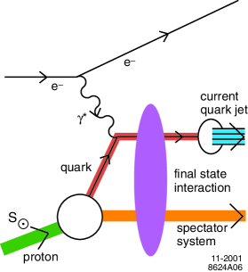
Figure 1: The final-state interaction in the semi-inclusive deep inelastic lepton scattering $\ell p^{\uparrow}\to\ell^{\prime}\pi X$.

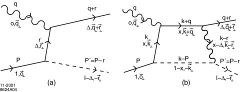
Figure 2: The tree (a) and one-loop (b) graphs for $\gamma^{*}p\to q(qq)_{0}$. The interference of the two amplitudes with $J^{z}_{p}=\pm{1/2}$ provides the proton’s single-spin asymmetry.

The amplitude for the $\gamma^{*}p\to q(qq)_{0}$ can be computed from the tree and one-loop graphs illustrated in Fig. 2. A spin asymmetry will arise from the final-state interactions of the outgoing charged lines. The $J^{z}=+{1\over 2}$ two-particle Fock state is given by [7, 8]

$$\left|\Psi^{\uparrow}_{\rm two\ particle}(P^{+},\vec{P}_{\perp}=\vec{0}_{\perp})\right>$$

$$= \int\frac{{\mathrm{d}}^{2}{\vec{k}}_{\perp}{\mathrm{d}}x}{{\sqrt{x(1-x)}}16\pi^{3}}\Big{[}\ \psi^{\uparrow}_{+\frac{1}{2}}(x,{\vec{k}}_{\perp})\,\left|+\frac{1}{2}\,;\,\,xP^{+}\,,\,\,{\vec{k}}_{\perp}\right>$$

$$\qquad+\psi^{\uparrow}_{-\frac{1}{2}}(x,{\vec{k}}_{\perp})\,\left|-\frac{1}{2}\,;\,\,xP^{+}\,,\,\,{\vec{k}}_{\perp}\right>\ \Big{]}\ ,$$

where

$$\left\{\begin{array}[]{l}\psi^{\uparrow}_{+\frac{1}{2}}(x,{\vec{k}}_{\perp})=(M+\frac{m}{x})\,\varphi\ ,\\ \psi^{\uparrow}_{-\frac{1}{2}}(x,{\vec{k}}_{\perp})=-\frac{(+k^{1}+{\mathrm{i}}k^{2})}{x}\,\varphi\ .\end{array}\right.$$ (2)

The scalar part of the wavefunction $\varphi$ depends on the dynamics. In the perturbative theory it is simply

$$\varphi=\varphi(x,{\vec{k}}_{\perp})=\frac{{e\over\sqrt{1-x}}}{M^{2}-{{\vec{k}}_{\perp}^{2}+m^{2}\over x}-{{\vec{k}}_{\perp}^{2}+\lambda^{2}\over 1-x}}\ .$$ (3)

In general one normalizes the Fock state to unit probability.

Similarly, the $J^{z}=-{1\over 2}$ two-particle Fock state has components

$$\left\{\begin{array}[]{l}\psi^{\downarrow}_{+\frac{1}{2}}(x,{\vec{k}}_{\perp})=\frac{(+k^{1}-{\mathrm{i}}k^{2})}{x}\,\varphi\ ,\\ \psi^{\downarrow}_{-\frac{1}{2}}(x,{\vec{k}}_{\perp})=(M+\frac{m}{x})\,\varphi\ .\end{array}\right.$$ (4)

The spin-flip amplitudes in (2) and (4) have orbital angular momentum projection $l^{z}=+1$ and $-1$ respectively. The numerator structure of the wavefunctions is characteristic of the orbital angular momentum, and holds for both perturbative and non-perturbative couplings.

We require the interference between the tree amplitude of Fig. 2a and the one loop graph of Fig. 2b. The contributing amplitudes for $\gamma^{*}p\to q(qq)_{0}$ have the following structure through one loop order:

$${\cal A}(\Uparrow\to\uparrow) = (M+{m\over\Delta})\ C\ (h+i{e_{1}e_{2}\over 8\pi}g_{1})$$ (5)

$${\cal A}(\Downarrow\to\uparrow) = \ ({+r^{1}-ir^{2}\over\Delta})\ \ C\ (h+i{e_{1}e_{2}\over 8\pi}g_{2})$$ (6)

$${\cal A}(\Uparrow\to\downarrow) = \ ({-r^{1}-ir^{2}\over\Delta})\ \ C\ (h+i{e_{1}e_{2}\over 8\pi}g_{2})$$ (7)

$${\cal A}(\Downarrow\to\downarrow) = (M+{m\over\Delta})\ C\ (h+i{e_{1}e_{2}\over 8\pi}g_{1})\ ,$$ (8)

where

$$C = -\ g\ e_{1}\ P^{+}\ {\sqrt{\Delta}}\ 2\ \Delta\ (1-\Delta)$$ (9)

$$h = {1\over{\vec{r}}_{\perp}^{2}+\Delta(1-\Delta)(-M^{2}+{m^{2}\over\Delta}+{\lambda^{2}\over 1-\Delta})}\ .$$ (10)

The quark light-cone fraction $\Delta={k^{+}\over P^{+}}$ is equal to the Bjorken variable $x_{bj}$ up to corrections of order $1/Q.$ The label $\Uparrow/\Downarrow$ corresponds to $J^{z}_{p}=\pm{1\over 2}.$ The second label $\uparrow/\downarrow$ gives the spin projection $J^{z}_{q}=\pm{1\over 2}$ of the spin-$\frac{1}{2}$  constituent. Here $e_{1}$ and $e_{2}$ are the electric charges of $q$ and $(qq)_{0}$, respectively, and $g$ is the coupling constant of the proton-$q$-$(qq)_{0}$ vertex. The first term in (5) to (8) is the Born contribution of the tree graph. The crucial result will be the fact that the contributions $g_{1}$ and $g_{2}$ from the one-loop diagram Fig. 2b are different, and that their difference is infrared finite. A gauge particle mass $\lambda_{g}$ will be used as an infrared regulator in the calculation of $g_{1}$ and $g_{2}.$

The calculation will be done using light-cone time-ordered perturbation theory, or equivalently, by integrating Feynman loop diagrams over $dk^{-}$. The light-cone frame used is $p=(p^{+},p^{-},\vec{p}_{\perp})=(P^{+},M^{2}/P^{+},\vec{0}_{\perp})$ and $q=(q^{+},q^{-},\vec{q}_{\perp})$ with $q^{+}=0$ and $q^{-}=2q\cdot p/P^{+}$, $\vec{q}_{\perp}=Q\hat{x}$ with $Q^{2}=-q^{2}$. The Bjorken variable is $\Delta=Q^{2}/2q\cdot p=Q^{2}/2M\nu.$ Since $q^{+}=0,$ light-cone time-orderings where the virtual photon produces a $q\overline{q}$ pair do not appear.

The light-cone formalism is invariant under boosts in the $\hat{z}$ direction: $P^{+}\to\gamma P^{+}$. It reduces to a laboratory frame when $P^{+}=M$. If we take $\vec{q}$ to lie in the $\hat{z}-\hat{x}$ plane in this frame, $\vec{q}=(q^{x},q^{y},q^{z})=(Q,0,-\nu)$; i.e., $\vec{q}$ is oriented at an angle $\theta_{lab}=\tan^{-1}{Q\over\nu,}$ from the negative $\hat{z}$ direction. This is illustrated in Fig. 3. Here $\nu$ is the laboratory energy of the photon. In the Bjorken scaling limit with $Q^{2}$ and $\nu$ large, and $\Delta=x_{bj}$ fixed, the angle $\theta_{lab}\to 0$, so the light-cone laboratory frame and usual laboratory frame with $\vec{q}$ taken in the $-\hat{z}$ direction are identical.

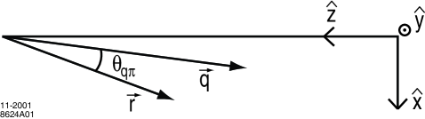
Figure 3: The light-cone frame used is $p=(p^{+},p^{-},\vec{p}_{\perp})=(P^{+},M^{2}/P^{+},\vec{0}_{\perp})$ and $q=(q^{+},q^{-},\vec{q}_{\perp})$ with $q^{+}=0$. The virtual photon and produced hadron define the production plane which we will take as the ${\hat{z}}-{\hat{x}}$ plane.

The covariant expression for the four one-loop amplitudes of diagram Fig. 2b is:

$${\cal A}^{\rm one-loop}(I)$$

$$= ig\ e_{1}^{2}\ e_{2}\ \int{d^{4}k\over(2\pi)^{4}}$$

$$\times{{\rm{\cal N}}(I)\over(k^{2}-m^{2}+i\epsilon)\ ((k+q)^{2}-m^{2}+i\epsilon)((k-r)^{2}-\lambda_{g}^{2}+i\epsilon)((k-P)^{2}-\lambda^{2}+i\epsilon)}$$

$$= -ig\ e_{1}^{2}\ e_{2}\ \int{d^{2}{\vec{k}}_{\perp}\over 2(2\pi)^{4}}\int P^{+}dx\ {{\rm{\cal N}}(I)\over P^{+4}\ x\ x\ (x-\Delta)\ (1-x)}\$$

$$\times\int dk^{-}{1\over\left(k^{-}-{(m^{2}+{\vec{k}}_{\perp}^{2})-i\epsilon\over xP^{+}}\right)\left((k^{-}+q^{-})-{(m^{2}+({\vec{k}}_{\perp}+{\vec{q}}_{\perp})^{2})-i\epsilon\over xP^{+}}\right)}$$

$$\times{1\over\left((k^{-}-r^{-})-{(\lambda_{g}^{2}+({\vec{k}}_{\perp}-{\vec{r}}_{\perp})^{2})-i\epsilon\over(x-\Delta)P^{+}}\right)\left((k^{-}-P^{-})+{(\lambda^{2}+{\vec{k}}_{\perp}^{2})-i\epsilon\over(1-x)P^{+}}\right)},\$$

where we used $k^{+}=xP^{+}.$ The numerators ${\rm{\cal N}}(I)$ are given by

$${\rm{\cal N}}(\Uparrow\to\uparrow) = 2P^{+}{\sqrt{\Delta}}\ x\ (M+{m\over x})\ q^{-}$$ (12)

$${\rm{\cal N}}(\Downarrow\to\uparrow) = 2P^{+}{\sqrt{\Delta}}\ x\ ({+k^{1}-ik^{2}\over x})\ q^{-}$$ (13)

$${\rm{\cal N}}(\Uparrow\to\downarrow) = 2P^{+}{\sqrt{\Delta}}\ x\ ({-k^{1}-ik^{2}\over x})\ q^{-}$$ (14)

$${\rm{\cal N}}(\Downarrow\to\downarrow) = 2P^{+}{\sqrt{\Delta}}\ x\ (M+{m\over x})\ q^{-}\ ,$$ (15)

where $q^{-}={Q^{2}\over\Delta P^{+}}={2M\nu\over P^{+}}\ .$ For the [current]-[gauge propagator]-[current] factor, in Feynman gauge only the $-g^{+-}$ term of the gauge propagator $-g^{\mu\nu}$ contributes in the Bjorken limit, and it provides a factor proportional to $q^{-}$ in the numerator which cancels the $q^{-}$ in the denominator of the gauge propagator. Therefore the result scales in the Bjorken limit.

The integration over $k^{-}$ in (2) does not give zero only if $0<x<1$. We first consider the region $\Delta<x<1$.

$${\cal A}^{\rm one-loop}(I)$$

$$= -ig\ e_{1}^{2}\ e_{2}\ \times\ (2\pi i)\ \int{d^{2}{\vec{k}}_{\perp}\over 2(2\pi)^{4}}\int P^{+}dx\ {{\rm{\cal N}}(I)\over P^{+4}\ x\ x\ (x-\Delta)\ (1-x)}\$$

$$\times{1\over\left(P^{-}-{(\lambda^{2}+{\vec{k}}_{\perp}^{2})-i\epsilon\over(1-x)P^{+}}-{(m^{2}+{\vec{k}}_{\perp}^{2})-i\epsilon\over xP^{+}}\right)\left(P^{-}-{(\lambda^{2}+{\vec{k}}_{\perp}^{2})-i\epsilon\over(1-x)P^{+}}+q^{-}-{(m^{2}+({\vec{k}}_{\perp}+{\vec{q}}_{\perp})^{2})-i\epsilon\over xP^{+}}\right)}$$

$$\times{1\over\left(P^{-}-{(\lambda^{2}+{\vec{k}}_{\perp}^{2})-i\epsilon\over(1-x)P^{+}}-r^{-}-{(\lambda_{g}^{2}+({\vec{k}}_{\perp}-{\vec{r}}_{\perp})^{2})-i\epsilon\over(x-\Delta)P^{+}}\right)},\$$

The result is identical to that obtained from light-cone time-ordered perturbation theory.

The phases $\chi_{i}$ needed for single-spin asymmetries come from the imaginary part of (2), which arises from the potentially real intermediate state allowed before the rescattering. The imaginary part of the propagator (light-cone energy denominator) gives

$$-i\pi \delta \left(P^{-}-{(\lambda^{2}+{\vec{k}}_{\perp}^{2})\over(1-x)P^{+}}+q^{-}-{(m^{2}+({\vec{k}}_{\perp}+{\vec{q}}_{\perp})^{2})\over xP^{+}}\right)$$ (17)

$$= \ -i\pi\ {1\over P^{+}}\ {\Delta^{2}\over{\vec{q}}_{\perp}^{2}}\ \delta(x\ -\ \Delta\ -\ {\overline{\delta}})\ ,$$

where

$${\overline{\delta}}\ =\ 2\ \Delta\ {{\vec{q}}_{\perp}\cdot({\vec{k}}_{\perp}-{\vec{r}}_{\perp})\over{\vec{q}}_{\perp}^{2}}\ .$$ (18)

Since the exchanged momentum $\overline{\delta}P^{+}$ is small, the light-cone energy denominator corresponding to the gauge propagator is dominated by the $({\vec{k}}_{\perp}-{\vec{r}}_{\perp})^{2}+\lambda^{2}_{g}\over(x-\Delta)$ term. This gets multiplied by $(x-\Delta)$, so only $({\vec{k}}_{\perp}-{\vec{r}}_{\perp})^{2}+\lambda^{2}_{g}$ appears in the propagator, independent of whether the photon is absorbed or emitted. The contribution from the region $0<x<\Delta$ thus compliments the contribution from the region $\Delta<x<1$.

We can integrate (2) over the transverse momentum using a Feynman parametrization to obtain the one-loop terms in (5) to (8).

$$g_{1} = \int_{0}^{1}d\alpha\ {1\over\alpha(1-\alpha){\vec{r}}_{\perp}^{2}+\alpha\lambda_{g}^{2}+(1-\alpha)\Delta(1-\Delta)(-M^{2}+{m^{2}\over\Delta}+{\lambda^{2}\over 1-\Delta})}$$ (19)

$$g_{2} = \int_{0}^{1}d\alpha\ {\alpha\over\alpha(1-\alpha){\vec{r}}_{\perp}^{2}+\alpha\lambda_{g}^{2}+(1-\alpha)\Delta(1-\Delta)(-M^{2}+{m^{2}\over\Delta}+{\lambda^{2}\over 1-\Delta})}\ .$$ (20)

Although not necessary for our analysis, we will assume for convenience that the final-state interactions generate a phase when exponentiated, as in the Coulomb phase analysis of QED. The rescattering phases $e^{i\chi_{i}}$ $(i=1,2)$ with $\chi_{i}={\rm tan}^{-1}({e_{1}e_{2}\over 8\pi}{g_{i}\over h})$ are thus distinct for the spin-parallel and spin-antiparallel amplitudes. The difference in phase arises from the orbital angular momentum $k_{\perp}$ factor in the spin-flip amplitude, which after integration gives the extra factor of the Feynman parameter $\alpha$ in the numerator of $g_{2}$. Notice that the phases $\chi_{i}$ are each infrared divergent for zero gauge boson mass $\lambda_{g}\to 0$, as is characteristic of Coulomb phases. However, the difference $\chi_{1}-\chi_{2}$ which contributes to the single-spin asymmetry is infrared finite. We have verified that the Feynman gauge result is also obtained in the light cone gauge using the principal value prescription. The small numerator coupling of the light-cone gauge particle is compensated by the small value for the exchanged $l^{+}=\overline{\delta}P^{+}$ momentum.

The virtual photon and produced hadron define the production plane which we will take as the ${\hat{z}}-{\hat{x}}$ plane. The azimuthal single-spin asymmetry transverse to the production plane is given by

$${\cal P}_{y} = {e_{1}e_{2}\over 8\pi}\ {2\ \Bigl{(}\ \Delta\,M+m\ \Bigr{)}\ r^{1}\over\Big{[}\ \Bigl{(}\ \Delta\,M+m\ \Bigr{)}^{2}\ +\ {\vec{r}}_{\perp}^{2}\ \Big{]}}\ \Big{[}\ {\vec{r}}_{\perp}^{2}+\Delta(1-\Delta)(-M^{2}+{m^{2}\over\Delta}+{\lambda^{2}\over 1-\Delta})\ \Big{]}$$ (21)

$$\times \ {1\over{\vec{r}}_{\perp}^{2}}\ {\rm ln}{{\vec{r}}_{\perp}^{2}+\Delta(1-\Delta)(-M^{2}+{m^{2}\over\Delta}+{\lambda^{2}\over 1-\Delta})\over\Delta(1-\Delta)(-M^{2}+{m^{2}\over\Delta}+{\lambda^{2}\over 1-\Delta})}\ .$$

The linear factor of $r^{1}=r^{x}$ reflects the fact that the single spin asymmetry is proportional to ${\vec{S}}_{p}\cdot\vec{q}\times\vec{r}$ where ${\vec{q}}\sim-\nu\hat{z}$ and ${\vec{S}}_{p}=\pm\hat{y}.$ Here $\Delta=x_{bj}$.

Our analysis can be generalized to the corresponding calculation in QCD. The final-state interaction from gluon exchange has the strength ${e_{1}e_{2}\over 4\pi}\to C_{F}\alpha_{s}(\mu^{2}).$ The scale of $\alpha_{s}$ in the ${\overline{MS}}$ scheme can be identified with the momentum transfer carried by the gluon $\mu^{2}=e^{-5/3}({\vec{k}}_{\perp}-{\vec{r}}_{\perp})^{2}$ [9]. The matrix elements of the proton to its constituents will have the same numerator structure as the perturbative model since they are determined by orbital angular momentum constraints. The strengths of the proton matrix elements can be normalized by the anomalous magnetic moment and the total charge. In QCD, $r_{\perp}$ is the magnitude of the momentum of the current quark jet relative to the virtual photon direction. Notice that for large $r_{\perp}$, ${\cal P}_{y}$ decreases as $\alpha_{s}(r^{2}_{\perp})x_{bj}Mr_{\perp}\ln r^{2}_{\perp}\over{r}_{\perp}^{2}$. The physical proton mass $M$ appears since it is present in the ratio of the $L_{z}=1$ and $L_{z}=0$ matrix elements. This form is expected to be essentially universal.

3 Model Predictions

We show the predictions of our model in Fig. 4 for the asymmetry ${\cal P}_{y}=A^{\sin\phi}_{UT}$ of the $i{\vec{S}}_{p}\cdot\vec{q}\times\vec{p}_{q}$ correlation based on Eq. (21). As representative parameters we take $\alpha_{s}=0.3$, $M=0.94$ GeV for the proton mass, $m=0.3$ GeV for the fermion constituent and $\lambda=0.8$ GeV for the spin-0 spectator. The single-spin asymmetry ${\cal P}_{y}$ is shown as a function of $\Delta$ at $r_{\perp}=0.5$ GeV in Fig. 4a and as a function of $r_{\perp}$ at $\Delta=0.15$ in Fig. 4b. The Hermes asymmetry $A_{UL}^{\sin\phi}$ contains a kinematic factor $K={Q\over\nu}\sqrt{1-y}={\sqrt{2Mx\over E}}{\sqrt{1-y\over y}}$ because the proton is polarized along the direction of the incident electron. The resulting predictions for $K{\cal P}_{y}$ are shown in Figs. 4c and 4d. Note that $\vec{r}=\vec{p}_{q}-\vec{q}$ is the momentum of the current quark jet relative to the photon direction. The asymmetry as a function of the pion momentum $\vec{p}_{\pi}$ requires a convolution with the quark fragmentation function.

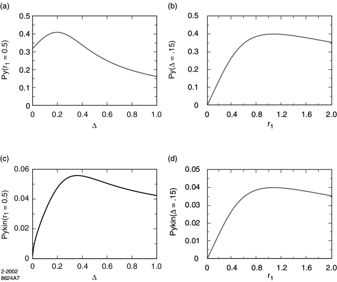
Figure 4: Model predictions for the single spin asymmetry of the proton in electroproduction resulting from gluon exchange in the final state as a function of $\Delta=x_{bj}$ and quark transverse momentum $r_{\perp}$. The parameters are given in the text.

4 Summary

We have calculated the single-spin asymmetry in semi-inclusive electroproduction induced by final-state interactions. We have shown that the final-state interactions from gluon exchange between the outgoing quark and the target spectator system leads to single-spin asymmetries in deep inelastic lepton-proton scattering at leading twist in perturbative QCD; i.e., the rescattering corrections are not power-law suppressed at large photon virtuality $Q^{2}$ at fixed $x_{bj}$. The azimuthal single-spin asymmetry ${\cal P}_{y}$ transverse to the photon-to-pion production plane decreases as $\alpha_{s}(r^{2}_{\perp})x_{bj}Mr_{\perp}[\ln r^{2}_{\perp}]/{r}_{\perp}^{2}$ for large $r_{\perp},$ where $r_{\perp}$ is the magnitude of the momentum of the current quark jet relative to the virtual photon direction. The fall-off in $r^{2}_{\perp}$ instead of $Q^{2}$ compensates for the dimension of the $\overline{q}$-$q$ -gluon correlation. The mass $M$ of the physical proton mass appears here since it determines the ratio of the $L_{z}=1$ and $L_{z}=0$ matrix elements. We have estimated the scale of $\alpha_{s}$ as ${\cal O}(r_{\perp}^{2}).$ The nominal size of the spin asymmetry is thus $C_{F}\alpha_{s}(r^{2}_{\perp})a_{p}$ where $a_{p}$ is the proton anomalous magnetic moment.

It is usually assumed that the cross section for semi-inclusive deep inelastic scattering at large $Q^{2}$ factorizes as the product of quark distributions times quark fragmentation functions [10, 11]. Our analysis shows that the single-spin asymmetry which arises from final-state interactions does not factorize in this way since the result depends on the $<p|\overline{\psi}_{q}A\psi|p>$ proton correlator, not the usual quark distribution derived from $<p|\overline{\psi}_{q}(\xi)\psi_{q}(0)|p>$ evaluated at equal light-cone time $\xi^{+}=0$. In particular, the spin asymmetry is not related to the transversity distribution $\delta q(x,Q)$ which correlates transversely polarized quarks with the spin of the transversely polarized target nucleon.

Our results are directly applicable to the azimuthal correlation of the proton spin with the virtual photon to current quark jet plane, which can be deduced from jet measures such as the thrust distribution. The $\sin\phi$ correlation of the proton spin with the photon-to-pion production plane as measured in the HERMES and SMC experiments can then be obtained using the usual fragmentation function. Detailed comparisons with experiment will be presented elsewhere. Our approach can also be applied to single-spin asymmetries in more general hadronic hard inclusive reactions such as $e^{+}e^{-}\to\Lambda^{\uparrow}X$ and $pp\to\Lambda^{\uparrow}X.$

Acknowledgments

We thank John Collins, Paul Hoyer, and Stephane Peigne for helpful comments.

References

• [1] HERMES Collaboration, A. Airapetian et al., Phys. Rev. Lett. 84, 4047 (2000); Phys. Rev. D64, 097101 (2001).
• [2] A. Bravar, for the SMC Collaboration, Nucl. Phys. B (Proc. Suppl.) 79, 520 (1999).
• [3] E704 Collaboration, A. Bravar et al., Phys. Rev. Lett. 77, 2626 (1996).
• [4] K. Heller, in Proceedings of Spin 96, C. W. de Jager, T. J. Ketel and P. Mulders, Eds., World Scientific (1997).
• [5] S. J. Brodsky, P. Hoyer, N. Marchal, S. Peigne and F. Sannino, hep-ph/0104291.
• [6] G. P. Lepage and S. J. Brodsky, Phys. Rev. D22, 2157 (1980); S. J. Brodsky and G. P. Lepage, in: Perturbative Quantum Chromodynamics, edited by A. H. Mueller (World Scientific, Singapore 1989).
• [7] S. J. Brodsky and S. D. Drell, Phys. Rev. D22, 2236 (1980).
• [8] S. J. Brodsky, D. S. Hwang, B. Q. Ma and I. Schmidt, Nucl. Phys. B 593, 311 (2001).
• [9] S. J. Brodsky, A. H. Hoang, J. H. Kühn and T. Teubner, Phys. Lett. B 359, 355 (1995).
• [10] J. C. Collins, Nucl. Phys. B 396, 161 (1993).
• [11] D. Boer and P. J. Mulders, Phys. Rev. D57, 5780 (1998).