The anomalous magnetic moment of the muon in the D-brane realization of the Standard Model

Abstract:

The anomalous magnetic moment of the muon is evaluated in the D-brane realization of the Standard Model. It is pointed out that the massive anomalous U(1) gauge bosons predicted, give extra contributions that are compatible with current experimental data.

1 Introduction

The recent precise measurement of the anomalous magnetic moment (AMM) of muon $\alpha_{muon}=(g-2)/2$ from the Brookhaven AGS experiment [1] gave

$$\alpha_{muon}^{exp}=116592023(151)\times 10^{-11}$$ (1)

The difference between the experimental value (1) and the theoretical expectation, (for a review see [2]), due to standard model (SM) is

$$\delta\alpha_{muon}=\alpha_{muon}^{exp}-\alpha_{muon}^{SM}=(43\pm 16)\times 10^{-10}.$$ (2)

The experimental precision is unprecented and it is going to reach $\pm 4\times 10^{-10}$ soon. It becomes thus important to examine the signals of physics beyond the SM. Various explanations for a discrepancy have been proposed building on earlier computations [4]. Many of those assume SUSY broken at a mass scale not far above the weak scale [7, 8, 9, 6, 10]. Other approaches include large or warped extra dimensional models, extended gauge structure and other alternatives [11, 12, 13, 14].

In this paper, we are pointing out that the experimental result (1) appears naturally in the D-brane realization of the SM in the context of orientifold vacua of string theory. String theory vacua with a very low string scale $M_{s}$ [18, 21, 20, 22, 23], and supersymmetry broken at that scale do not suffer directly from the ordinary hierarchy problem of the scalar masses [19, 20]. Rather, the hierarchy problem transmutes into the question as to why four-dimensional gravity is so weak. Moreover, if the string scale is around a few TeV, observation of novel effects at the near future experiments becomes a realistic possibility. A low string scale compatible with the known value of the Planck scale can be easily accommodated in ground states of unoriented open and closed strings. Solvable vacua of this type are orientifolds of closed strings. Such vacua include various type of D-branes stretching their worldvolumes in the four non-compact dimensions while wrapping additional worldvolume dimensions around cycles of the compact six torus. Moreover, they include non-dynamical orientifold planes that cancel the charges of the D-branes, implementing the (un)orientability condition and stabilizing the vacuum (cancellation of tadpoles).

Gauge interactions are described by open strings whose ends are confined on the D-branes, while gravity is mediated by closed strings in the bulk [20]. Ordinary matter is preferably generated by the fluctuations of the open strings and is thus also localized on the appropriate D-branes. The observed hierarchy between the Planck and the weak scale is accounted for by two or more large dimensions, transverse to our brane-world. Since the masses of the SM matter are well below the string scale, the branes on which the SM fields are located must be close together in the internal transverse compact space. Thus, for some questions, it makes sense to study this local configuration of branes without direct reference to the global groundstate configuration. Questions of ground state stability on the other hand are global questions.

In [27], the local D-brane configuration that can reproduce the SM fields was presented. The brane gauge-group is $U(3)\times U(2)\times U(1)$ and strong and electroweak apartinteractions arise from two different collections of coincident branes, leading to different gauge couplings. The hypercharge is a linear combination of the abelian factors of the gauge group. All such hypercharge embeddings were classified in [27]. The abelian gauge symmetries orthogonal to the hypercharge are “anomalous”, their anomaly cancelled by a Green-Schwarz mechanism [24, 25]. Such gauge symmetries are broken at the string scale, the gauge bosons becoming massive. The electroweak gauge symmetry is broken by the vacuum expectation values of two Higgs doublets, which are both necessary to give masses to all quarks and leptons. Moreover, the minimal spectrum can be completely non-supersymmetric. In such a case matching with the SM predicts that the string scale is in the range 6-8 TeV [27]. Several orientifold models as well as local brane configurations that come close to the SM have been described in the literature [26].

In the gauge sector the only free parameters, not fixed by the anomalies, are the masses of the two anomalous gauge bosons. These are of the order of the string scale. Their precise values can be obtained by a one-loop string calculation [30] once a concrete string model exists. Such masses are proportional to $g_{i}M_{s}$, where the $g_{i}$ are the gauge couplings, consequently we expect that they are in the region of a few TeV.

In this minimal realization, the only extra low-lying states from the standard model fields are the two massive “anomalous” gauge bosons. The particles couple minimally to the leptons with strengths that are fixed by the known gauge couplings. Thus, they provide computable contributions to the anomalous magnetic moment of the muon, the only uncertainty coming from the uncertainty in their masses

In this paper we compute such $(g-2)_{\rm anom}$ contributions and show that they are in the range implied by the experimental result. We use (1) to provide precise constrains for the masses of the anomalous U(1)’s in the TeV range.

The structure of this paper is as follows: In section two we describe in more detail the main features of the D-brane realization of the SM. In section three we describe the essential ingredients of the one-loop diagrammatic calculation of $(g-2)_{\rm anom}$. In section four the calculation of $(g-2)_{\rm anom}$ is done for the D-SM. Section five contains our conclusions and further comments. In appendix A we describe the precise field theoretic Lagrangian of the D-SM. In appendix B details of the diagrammatic calculations and proof of the gauge invariance of the result can be found.

2 The D-brane realization of SM

The simplest way the $SU(3)\times SU(2)\times U(1)$ gauge group of the SM can be embedded in a product of unitary groups appearing on D-brane stacks is as a subgroup of $U(3)\times U(2)\times U(1)$. A U(n) factor arises from n coincident D-branes. As $U(3)=SU(3)\times U(1)$, a string with one end on this group of branes is a triplet under $SU(3)$ with $Q_{3}=\pm 1$ abelian charge. Thus, $Q_{3}$ is identified with the gauged baryon number. Similarly, the second factor arises from two coincident D-branes (”weak” branes) and the gauged overall abelian charge $Q_{2}$ is identified with the weak-doublet number. Both collections have their own gauge couplings $g_{3}$, $g_{2}$ that are functions of the string coupling $g_{s}$ and possible compactification volumes. The necessity for the extra $U(1)$ factor is due to the fact that we cannot express the hypercharge as a linear combination of baryon and weak-doublet numbers . The U(1) brane can be in principle independent of the other branes and has in general a different gauge coupling $g_{1}$. In [27], the $U(1)$ brane has been put on top of either the color or the weak D-branes. Thus, $g_{1}$ is equal to either $g_{3}$ or $g_{2}$.

Let us denote by $Q_{3}$, $Q_{2}$ and $Q_{1}$ the three $U(1)$ charges of $U(3)\times U(2)\times U(1)$. These charges can be fixed so that they lead to the right hypercharge. In order that we can match the measured gauge couplings with the ones appropriate for the brane-configuration and also avoid hierarchy problems we find that we have to put the $U(1)$ brane on top of the color branes. Consequently we set $g_{1}=g_{3}$. This fixes the string scale to be between 6 to 8 TeV [27]. There are two possibilities for charge assignments. Under $SU(3)\times SU(2)\times U(1)_{3}\times U(1)_{2}\times U(1)_{1}$ the members of a given quark and lepton family have the following quantum numbers:

$$Q ({\bf 3},{\bf 2};1,1+2z,0)_{1/6}$$

$$u^{c} ({\bf\bar{3}},{\bf 1};-1,0,0)_{-2/3}$$

$$d^{c} ({\bf\bar{3}},{\bf 1};-1,0,1)_{1/3}$$

$$L ({\bf 1},{\bf 2};0,1,z)_{-1/2}$$

$$l^{c} ({\bf 1},{\bf 1};0,0,1)_{1}$$

where $z=0,-1$. From (2) and the requirement that the Higgs doublet has hypercharge 1/2, one finds two possible assignments for it:

$$H\ \ ({\bf 1},{\bf 2};0,1+2z,1)_{1/2}\quad H^{\prime}\ \ ({\bf 1},{\bf 2};0,-(1+2z),0)_{1/2}$$ (4)

The trilinear Yukawa terms are

$$z=0\ :\qquad H^{\prime}Qu^{c}\ \quad H^{\dagger}Ll^{c}\ ,\quad H^{\dagger}Qd^{c}$$ , (5)

$$z=-1\ :\qquad H^{\prime}Qu^{c}\ \quad H^{\prime\dagger}Ll^{c}\ ,\quad H^{\dagger}Qd^{c}$$ , (6)

In each case, two Higgs doublets are necessary to give masses to all quarks and leptons. The U(3) and U(1) branes are D3 branes. The U(2) branes are D7 branes whose four extra longitudinal directions are wrapped on a four-torus of volume 2.5 in string units [27]. The spectator U(1)_b brane is stretching in the bulk but the fermions that end on it do not have KK excitations. Thus, the only SM field that has KK excitations is a linear combination of the hypercharge gauge boson and the two anomalous U(1) gauge bosons. The masses of KK states, are shifted from the basic state by multiples of $0.8M_{s}$.

We will now describe the structure of the gauge sector for the D-brane configuration above. We denote by $A^{i}_{\mu}$ the $U(1)_{i}$ gauge fields and $F^{i}_{\mu\nu}$ their corresponding field strengths. Also we denote $G^{\beta}_{\mu\nu}$ the field strengths of the non-abelian gauge group where $\beta$ runs over the two simple factors. There is also a set of two axion fields $b^{\alpha}$ with normalized kinetic terms. Starting from the kinetic terms of the gauge fields and requesting for the cancellation of the $QT^{\alpha}T^{\alpha}$ mixed anomalies, we can write down the most general low energy action

$${\cal L}= - {1\over 4}\sum_{i}F^{i}_{\mu\nu}F^{i,\mu\nu}+\sum_{i}\bar{\psi}Q_{i}\raise 0.6458pt\hbox{$/$}\kern-5.70007pt{A^{i}}\psi-{1\over 4}\sum_{a}TrG^{a}_{\mu\nu}G^{a,\mu\nu}$$

$$+ \sum_{\alpha,\beta}\Lambda_{\alpha,\beta}{b^{\alpha}\over M_{s}}\epsilon^{\mu\nu\rho\sigma}Tr[G^{\beta}_{\mu\nu}G^{\beta}_{\rho\sigma}]+\sum_{\alpha}(\partial_{\mu}b^{\alpha}-M_{s}\lambda^{\alpha i}A^{i}_{\mu})(\partial^{\mu}b^{\alpha}-M_{s}\lambda^{\alpha j}A^{j,\mu})$$

$$+ \sum_{\alpha,i,j}{C_{\alpha ij}\over M_{s}}\epsilon^{\mu\nu\rho\sigma}\partial_{\mu}b^{\alpha}A^{i}_{\nu}F^{j}_{\rho\sigma}+\sum_{i,j,k}{D_{ijk}\over M_{s}}\epsilon^{\mu\nu\rho\sigma}A^{i}_{\mu}A^{j}_{\nu}F^{k}_{\rho\sigma}$$

$$+ \sum_{\alpha}Z_{\alpha}{b^{\alpha}\over M_{s}}\epsilon^{\mu\nu\rho\sigma}Tr[R_{\mu\nu}R_{\rho\sigma}]$$

where charge operators $Q_{i}$ contain all coupling dependence. The last term involves the curvature two-form $R_{\mu\nu}$ and is responsible for the cancellation of the gravitational anomalies. Under $U(1)$ gauge transformations (modified by the anomaly)

$$A^{i}_{\mu}\rightarrow A^{i}_{\mu}+\partial_{\mu}\epsilon^{i}\quad,\quad b^{\alpha}\rightarrow b^{\alpha}+\sum_{i}\lambda^{\alpha i}A^{i}_{\mu}$$ (8)

we have

$$D_{ijk}=-D_{jik}\quad,\quad\sum_{a}\Lambda_{\alpha,\beta}\lambda^{\alpha,\iota}=Tr[Q^{i}T_{\beta}T_{\beta}]$$ (9)

$$D_{ijk}=-\sum_{a}C_{\alpha ij}\lambda^{\alpha k}=Tr[Q^{i}Q^{j}Q^{k}]\quad,\quad\sum_{a}Z_{\alpha}\lambda^{\alpha,i}=Tr[Q^{i}]$$ (10)

The only free parameters which are not fixed by the anomalies are $\lambda^{\alpha i}$. These define the mass matrix of gauge bosons $M^{2}_{ij}=M^{2}_{s}\lambda^{\alpha i}\lambda^{bj}$. This matrix is symmetric and has a zero eigenvalue corresponding to the non-anomalous hypercharge. The $\lambda^{\alpha i}$ can be computed by a string calculation. The parameters remaining in the mass matrix is the $2\times 2$ submatrix of the anomalous gauge bosons.

Now, we will describe the couplings of the gauge fields in more details. The two first terms of (2) are written as

$${\cal L}=-{1\over 4}\sum_{i}F^{i}F^{i}+\sum_{i}{g_{i}\over\sqrt{i}}\bar{\psi}Q_{i}\raise 0.6458pt\hbox{$/$}\kern-5.70007pt{A^{i}}\psi$$ (11)

where $g_{i}$ are the $SU(i)$ coupling constants and the charges have the standard integral normalization (2). We will set $x={g_{3}/\sqrt{3}\over g_{2}/\sqrt{2}}=\sqrt{5/3}$ as $g_{2}/g_{3}\sim\sqrt{0.4}$ [27]. Doing a $O(3)$ rotation, we can go to a basis where the kinetic terms of the $U(1)$ gauge fields are still diagonal, while one of them corresponds to the hypercharge: $A_{i}=U_{ij}\widetilde{A}_{j}$ with $A_{Y}=\widetilde{A}_{1}$. This rotation is different in each theory.

For the $z=0$ case we use

$$U=\left(\begin{array}[]{ccc}{2\sqrt{3}\over\sqrt{28+9x^{2}}}&-{\sqrt{16+9x^{2}}\sin{\theta}\over\sqrt{28+9x^{2}}}&{\sqrt{16+9x^{2}}\sin{\theta}\sqrt{3}\over\sqrt{28+9x^{2}}}\\ -{3x\over\sqrt{28+9x^{2}}}&-{2(-2\sqrt{28+9x^{2}}\cos{\theta}+3\sqrt{3}x\sin{\theta})\over\sqrt{28+9x^{2}}\sqrt{16+9x^{2}}}&{2(2\sqrt{28+9x^{2}}\sin{\theta}+3\sqrt{3}x\cos{\theta})\over\sqrt{28+9x^{2}}\sqrt{16+9x^{2}}}\\ {4\over\sqrt{28+9x^{2}}}&{3x\sqrt{28+9x^{2}}\cos{\theta}+8\sqrt{3}\sin{\theta}\over\sqrt{28+9x^{2}}\sqrt{16+9x^{2}}}&{3x\sqrt{28+9x^{2}}\sin{\theta}-8\sqrt{3}\cos{\theta}\over\sqrt{28+9x^{2}}\sqrt{16+9x^{2}}}\end{array}\right)$$ (12)

and the $U(1)$ charges:

$$Q_{Y}\sim Q_{1}-{Q_{2}\over 2}+{2Q_{3}\over 3}$$

$$Q_{\alpha}\sim-\sqrt{3}x(16+9x^{2})\sin{\theta}Q_{1}+2(2\sqrt{28+9x^{2}}\cos{\theta}-3\sqrt{3}x\sin{\theta})Q_{2}+$$

$$+(3x^{2}\sqrt{28+9x^{2}}\cos{\theta}+8\sqrt{3}x\sin{\theta})Q_{3}$$ (13)

$$Q_{b}\sim\sqrt{3}x(16+9x^{2})\cos{\theta}Q_{1}+2(2\sqrt{28+9x^{2}}\sin{\theta}+3\sqrt{3}x\cos{\theta})Q_{2}+$$

$$+(3x^{2}\sqrt{28+9x^{2}}\sin{\theta}-8\sqrt{3}x\cos{\theta})Q_{3}$$

We can obtain the $z=-1$ case from the one above by $x\rightarrow-x$. The matrix $U$ is now

$$U=\left(\begin{array}[]{ccc}{2\sqrt{3}\over\sqrt{28+9x^{2}}}&-{\sqrt{16+9x^{2}}\sin{\theta}\over\sqrt{28+9x^{2}}}&{\sqrt{16+9x^{2}}\sin{\theta}\sqrt{3}\over\sqrt{28+9x^{2}}}\\ {3x\over\sqrt{28+9x^{2}}}&{2(2\sqrt{28+9x^{2}}\cos{\theta}+3\sqrt{3}x\sin{\theta})\over\sqrt{28+9x^{2}}\sqrt{16+9x^{2}}}&-{2(-2\sqrt{28+9x^{2}}\sin{\theta}+3\sqrt{3}x\cos{\theta})\over\sqrt{28+9x^{2}}\sqrt{16+9x^{2}}}\\ {4\over\sqrt{28+9x^{2}}}&{-3x\sqrt{28+9x^{2}}\cos{\theta}+8\sqrt{3}\sin{\theta}\over\sqrt{28+9x^{2}}\sqrt{16+9x^{2}}}&-{3x\sqrt{28+9x^{2}}\sin{\theta}+8\sqrt{3}\cos{\theta}\over\sqrt{28+9x^{2}}\sqrt{16+9x^{2}}}\end{array}\right)$$ (14)

and the charges:

$$Q_{Y}\sim Q_{1}+{Q_{2}\over 2}+{2Q_{3}\over 3}$$

$$Q_{\alpha}\sim-\sqrt{3}x(16+9x^{2})\sin{\theta}Q_{1}+2(2\sqrt{28+9x^{2}}\cos{\theta}+3\sqrt{3}x\sin{\theta})Q_{2}+$$

$$+(-3x^{2}\sqrt{28+9x^{2}}\cos{\theta}+8\sqrt{3}x\sin{\theta})Q_{3}$$ (15)

$$Q_{b}\sim\sqrt{3}x(16+9x^{2})\cos{\theta}Q_{1}+2(2\sqrt{28+9x^{2}}\sin{\theta}-3\sqrt{3}x\cos{\theta})Q_{2}-$$

$$-(3x^{2}\sqrt{28+9x^{2}}\sin{\theta}-8\sqrt{3}x\cos{\theta})Q_{3}$$

The parameter $\theta$ can be used to diagonalize the mass matrix of the two anomalous $U(1)$s $A_{\alpha}$ and $A_{b}$. The two eigenvalues $\mu_{\alpha}^{2}$, $\mu_{b}^{2}$ and $\theta$ parametrize effectively the $2\times 2$ mass matrix. The masses of the anomalous $U(1)$ gauge fields have also contributions from the Higgs effect since the Higgses are also charged under the anomalous $U(1)$s. We evaluate these in appendix A. However, such corrections are of order of $m_{Z}/M_{s}$ and are thus subleading for our purposes. String theory calculations indicate that $\mu_{\alpha,b}$ are a factor of 5-10 below the string scale [30]. Thus they are expected to be in the TeV range.

3 Calculation of lepton anomalous magnetic moment in the presence of an anomalous $U(1)$

In order to describe the calculation and its subtleties we will first consider a toy model with a photon A, an anomalous $U(1)$ gauge field $B$, chiral charged fermions and a complex Higgs. We also have an axion $b$ to cancel the anomalies. We denote by ${\cal L}_{QED}$ the electrodynamics Lagrangian of the photon. The relevant part of the low-energy effective Lagrangian can be written as:

$${\cal L}={\cal L}_{QED} - {1\over 4}F^{2}+M_{s}^{2}(\partial b+B)^{2}+D_{\mu}HD^{\mu}H^{*}+V(|H|^{2})$$ (16)

$$+ Q_{L}\bar{\psi}_{L}\raise 0.6458pt\hbox{$/$}\kern-5.70007pt{B}\psi_{L}+Q_{R}\bar{\psi}_{R}\raise 0.6458pt\hbox{$/$}\kern-5.70007pt{B}\psi_{R}+h\bar{\psi}_{L}\psi_{R}H+c.c.$$

were $B_{\mu}$ is the anomalous $U(1)$ with field strength $F_{\mu\nu}$. This Lagrangian (16) is invariant under the “anomalous” $U(1)$ transformations.

$$B^{\mu} \rightarrow B^{\mu}+\partial^{\mu}\epsilon$$

$$\psi_{L} \rightarrow e^{iQ_{L}\epsilon}\psi_{L}$$

$$\psi_{R} \rightarrow e^{iQ_{R}\epsilon}\psi_{R}$$ (17)

$$H \rightarrow e^{i(Q_{R}-Q_{L})\epsilon}H$$

$$b \rightarrow b-\epsilon$$

There are two sources of gauge symmetry breaking. One is the stringy mass term and the other is the non-zero expectation value of the Higgs. Writing $H=re^{i\phi}$, the Higgs potential fixes the vacuum expectation value $<r>=v$. The kinetic term of the Higgs field gives an extra contribution to the B mass term:

$$v^{2}(\partial\phi+\Delta QB)^{2}$$ (18)

To proceed with the one-loop calculation, it is necessary to add a gauge fixing term

$${\cal L}_{gaugefixing}=\lambda\Big{(}\partial B+{cM_{s}^{2}\alpha\over{\lambda}}-{\Delta Qv^{2}\phi\over\lambda}\Big{)}^{2}$$ (19)

which keeps $B_{\mu}$ orthogonal to $b$ and $\phi$. Redefining $\tilde{b}=Mb$ and $\tilde{\phi}=v\phi$ we can diagonalize the axions doing a $SO(2)$ rotation

$$\left(\begin{array}[]{c}b^{\prime}\\ \phi^{\prime}\end{array}\right)=\left(\begin{array}[]{cc}\cos\theta^{\prime}&\sin\theta^{\prime}\\ -\sin\theta^{\prime}&\cos\theta^{\prime}\end{array}\right)\left(\begin{array}[]{c}\tilde{b}\\ \tilde{\phi}\end{array}\right)$$ (20)

where $\cos\theta^{\prime}={cM_{s}\over\sqrt{c^{2}M_{s}^{2}+v^{2}\Delta Q^{2}}}$ and $\sin\theta^{\prime}={\Delta Qv\over\sqrt{c^{2}M_{s}^{2}+v^{2}\Delta Q^{2}}}$. Now, the effective Lagrangian has the form

$${\cal L}={\cal L}_{ED} - {1\over 4}F_{B}^{2}+(c^{2}M_{s}^{2}+\Delta Q^{2}v^{2})B^{2}$$

$$+ (\partial b^{\prime})^{2}+{c^{2}M_{s}^{2}+\Delta Q^{2}v^{2}\over\lambda}b^{\prime 2}+(\partial\phi^{\prime})^{2}$$

$$+ Q_{L}\bar{\psi}_{L}\raise 0.6458pt\hbox{$/$}\kern-5.70007pt{B}\psi_{L}+Q_{R}\bar{\psi}_{R}\raise 0.6458pt\hbox{$/$}\kern-5.70007pt{B}\psi_{R}$$

$$+ hv\bar{\psi}_{L}\psi_{R}e^{i(\sin\theta^{\prime}b^{\prime}+\cos\theta^{\prime}\phi^{\prime})/v}+c.c.$$

The masses are:

$$m_{\psi} = hv$$

$$m_{B} = \sqrt{c^{2}M_{s}^{2}+v^{2}{\Delta Q}^{2}}$$

$$m_{\phi^{\prime}} = 0$$ (22)

$$m_{b^{\prime}} = \sqrt{c^{2}M_{s}^{2}+v^{2}{\Delta Q}^{2}}/\sqrt{\lambda}.$$

We define $m_{B}=\mu$ for simplicity. The Yukawa interactions are given by:

$$iQ_{L}\gamma_{\mu}\Big{(}{1-\gamma_{5}\over 2}\Big{)} \psi_{L} \psi_{L} B^{\mu}$$ ,

$$iQ_{R}\gamma_{\mu}\Big{(}{1+\gamma_{5}\over 2}\Big{)} \psi_{R} \psi_{R} B^{\mu}$$ ,

$${m\Delta Q\over\mu}\gamma_{5} \psi \psi b^{\prime}$$ ,

$${hcM_{s}\over\mu}\gamma_{5} \psi \psi \phi^{\prime}$$ ,

The propagators are:

$$D_{B}^{\mu\nu}(k)={-ig^{\mu\nu}\over{k^{2}-\mu^{2}}}+(1-\lambda^{-1}){ik^{\mu}k^{\nu}\over(k^{2}-\mu^{2})(k^{2}-\mu^{2}/{\lambda})}$$

$$G_{\phi^{\prime}}(k)={i\over k^{2}}$$ (23)

$$G_{b^{\prime}}(k)={i\over k^{2}-\mu^{2}/{\lambda}}$$

To derive the AMM of a lepton, we consider the three-point function of two leptons and a photon where a gauge boson or the two scalars can be exchanged on the internal line:

We sandwich the above diagram between two on-shell spinors, so we can use the Gordon decomposition and the mass-shell conditions. Our goal is to write the expression in the form:

$$\bar{u}(p^{\prime})\Big{\{}\gamma_{\mu}F_{1}(q^{2})+{i\sigma_{\mu\nu}q^{\nu}\over 2m}F_{2}(q^{2})\Big{\}}u(p)$$ (24)

where $q_{\mu}=p^{\prime}_{\mu}-p_{\mu}$. The $F_{2}(q^{2}=0)$ will give us a correction of the AMM of the lepton which propagates. In the present calculation, we have to include diagrams which are coming from the non trivial couplings between the anomalous $U(1)$s and leptons. The external vector gauge abelian field is the photon, the internal propagating fields with momentum $k$ can be the anomalous $U(1)$ gauge boson or the scalars (axions). We will outline here these calculations. More details can be found in appendix B.

As the anomalous $U(1)$ couples differently to left and right leptons, it is neccesary to consider diagrams where chirality is conserved (L-L, R-R diagrams) and others where chirality is different (L-R, R-L). The corresponding diagrams is

and in algebraic form:

$$\bar{u}(p^{\prime})[\int{d^{4}k\over(2\pi)^{4}}(iQ_{s}\gamma_{\nu}P_{s}){i\over\raise 0.6458pt\hbox{$/$}\kern-5.70007pt{p^{\prime}}-\raise 0.6458pt\hbox{$/$}\kern-5.70007pt{k}-m}\gamma_{\mu}{i\over\raise 0.6458pt\hbox{$/$}\kern-5.70007pt{p}-\raise 0.6458pt\hbox{$/$}\kern-5.70007pt{k}-m}(iQ_{l}\gamma_{\rho}P_{l})D^{\nu\rho}(k)]u(p)$$ (25)

where $s,l=L,R$ label the chirality.

The propagator of $U(1)$ contains the arbitrary gauge fixing parameter $\lambda$. In a non-chiral theory $\lambda$ disappears because of the mass-sell conditions of the two spinors which sandwich the diagrams (25). In a chiral theory, we need the contribution of $b^{\prime}$ with mass (22) in order to obtain a gauge invariant result. We also have to add the one-loop diagrams of $\phi^{\prime}$. These diagrams are:

where “axion” stands for $b^{\prime}$ or $\phi^{\prime}$. In algebraic form they are given by:

$${m^{2}\Delta Q^{2}\over\mu^{2}}\bar{u}(p^{\prime})\int{d^{4}k\over(2\pi)^{4}}\gamma_{5}{i\over\raise 0.6458pt\hbox{$/$}\kern-5.70007pt{p^{\prime}}-\raise 0.6458pt\hbox{$/$}\kern-5.70007pt{k}-m}\gamma_{\mu}{i\over\raise 0.6458pt\hbox{$/$}\kern-5.70007pt{p}-\raise 0.6458pt\hbox{$/$}\kern-5.70007pt{k}-m}\gamma_{5}G_{b^{\prime}}(k)u(p)$$ (26)

for the $b^{\prime}$ axion and

$${(hc)^{2}M_{s}^{2}\over\mu^{2}}\bar{u}(p^{\prime})\int{d^{4}k\over(2\pi)^{4}}\gamma_{5}{i\over\raise 0.6458pt\hbox{$/$}\kern-5.70007pt{p^{\prime}}-\raise 0.6458pt\hbox{$/$}\kern-5.70007pt{k}-m}\gamma_{\mu}{i\over\raise 0.6458pt\hbox{$/$}\kern-5.70007pt{p}-\raise 0.6458pt\hbox{$/$}\kern-5.70007pt{k}-m}\gamma_{5}G_{\phi^{\prime}}(k)u(p)$$ (27)

for $\phi^{\prime}$. We expect the sum of the three diagrams to be $\lambda$-independent. In Appendix B we show this explicitly. In view of this, we can use any gauge for the evaluation. For simplicity, we choose the Feynman - t’Hooft gauge $\lambda=1$

The steps of this calculation are as follow:

a) Express the denominator as a perfect square using the Feynman parameter trick and shifting the loop momentum.

b) Move all the $\raise 0.6458pt\hbox{$/$}\kern-5.70007pt{p^{\prime}}$ to the left, all the $\raise 0.6458pt\hbox{$/$}\kern-5.70007pt{p}$ to the right and make use of the on-shell spinor conditions.

c) Perform the momentum integral of the loop after a Wick rotation to Euclidean space.

d) Distinguish terms proportional to $p_{\mu}$ and $p^{\prime}_{\mu}$.

e) Integrate the remaining variables that resulted from Feynman parameter trick.

Following the steps above, we find for the anomalous $U(1)$ exchanged diagram (details can be found in Appendix B): For L-L and R-R diagrams:

$$-{Q_{L}^{2}+Q_{R}^{2}\over 16m\pi^{2}}(p_{\mu}+p^{\prime}_{\mu})\int_{0}^{1}dx{x(x^{2}-3x+2)\over x^{2}+(1-x){\mu^{2}\over m^{2}}}$$ (28)

For mixed diagrams (L-R and R-L):

$$-{Q_{L}Q_{R}\over 16m\pi^{2}}(p_{\mu}+p^{\prime}_{\mu})\int_{0}^{1}dx{2x(1-x)\over x^{2}+(1-x){\mu^{2}\over m^{2}}}$$ (29)

The axion $b^{\prime}$ exchange diagram gives

$${\Delta Q^{2}\over 16m\pi^{2}}{m^{2}\over\mu^{2}}(p_{\mu}+p^{\prime}_{\mu})\int_{0}^{1}dx{x^{3}\over x^{2}+(1-x){\mu^{2}\over m^{2}}}$$ (30)

The diagram for the axion $\phi^{\prime}$ has the same integral with (30) in the limit $\mu\rightarrow 0$. Since however the axion is expected to get a small mass from non-perturbative effects we will consider it with $m_{\phi^{\prime}}$ small. In this case we obtain

$${(hc)^{2}\over 16m\pi^{2}}{M_{s}^{2}\over\mu^{2}}(p_{\mu}+p^{\prime}_{\mu})\int_{0}^{1}dx{x^{3}\over x^{2}+(1-x){m_{\phi^{\prime}}^{2}\over m^{2}}}$$ (31)

As $M_{s}/\mu\sim 1$, the limit of (31) for $m_{\phi^{\prime}}\rightarrow 0$ is:

$${h^{2}\over 16m\pi^{2}}(p_{\mu}+p^{\prime}_{\mu}){1\over 2}$$ (32)

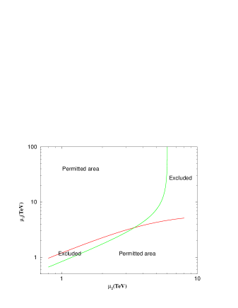
Figure 1: The $z=0$ model. Between the two plots is the excluded area, where the determinant of the second order equation is negative.

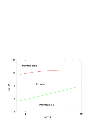
Figure 2: The $z=-1$ model. Between the two plots is the excluded area where the determinant of the second order equation is negative.

4 Anomalous magnetic moment of muon in the D-brane realization of the standard model

Using the results above we can now embark in the calculation of the AMM of the muon in the D-brane realization of the SM. To do this we have to include the contribution of (28) and (29) for both anomalous $U(1)$s as well as the (30) and (32) for the axion diagrams to the SM result.

$$\delta\alpha= {1\over 8\pi^{2}}\sum_{i=\alpha,b}\Big{(}{m\over\mu_{i}}\Big{)}^{2}\int_{0}^{1}dx{x(m^{2}\Delta Q_{i}^{2}x^{2}+\mu_{i}^{2}(4Q_{iL}Q_{iR}-(2-x)(Q^{2}_{iL}+Q^{2}_{iR}))(1-x)\over m^{2}x^{2}+\mu_{i}^{2}(1-x^{2})}$$ (33)

$$+{h^{2}\over 16\pi^{2}}$$

In our case $\mu_{i}\gg m$, therefore we expand the contributions and keep the terms up to second order in $(\mu_{i}/m)$. The final result is

$$\alpha^{U(3)\times U(2)\times U(1)}_{muon}=\alpha^{SM}_{muon}+\sum_{i=\alpha,b}{Q_{iL}^{2}-3Q_{iL}Q_{iR}+Q_{iR}^{2}\over 12\pi^{2}}\Big{(}{m\over\mu_{i}}\Big{)}^{2}+{h^{2}\over 16\pi^{2}}$$ (34)

where $Q_{\alpha L},Q_{\alpha R},Q_{bL},Q_{bL}$ are the rotated by (13) or (15), charges of (2). We use as $Q_{iL}$ and $Q_{iR}$ the charges of the $L$ and $l^{c}$ in (2).

Using the measured difference (2) we can express one of the unknown variables as a function of the two others. Thus, for $z=0$ we can find the $\mu_{\alpha}$ and $\mu_{\beta}$ dependence of $\tan\theta$. We have to solve a second order equation:

$$(12\pi^{2}\mu_{\alpha}^{2}\mu_{b}^{2}(\delta\alpha-\alpha_{\phi^{\prime}})+m^{2}(817\mu_{\alpha}^{2}-1220\mu_{b}^{2}))\tan^{2}\theta+26\sqrt{215}m^{2}(\mu_{\alpha}^{2}-\mu_{b}^{2})\tan\theta$$

$$+12\pi^{2}\mu_{\alpha}^{2}\mu_{b}^{2}(\delta\alpha-\alpha_{\phi^{\prime}})-1220m^{2}\mu_{\alpha}^{2}+817m^{2}\mu_{b}^{2} =0$$

where we denote as $\alpha_{\phi^{\prime}}$ the contribution from the axion $\phi^{\prime}$. As $\tan\theta$ is real, the discriminant must be positive. We can easily find the excluded area in the $\mu_{2}$,$\mu_{3}$ plane where this discriminant is negative. In Fig. 1 we plot this area for the z=0 model.

For the $z=-1$ model we obtain

$$(12\pi^{2}\mu_{\alpha}^{2}\mu_{b}^{2}(\delta\alpha-\alpha_{\phi^{\prime}})-m^{2}(10363\mu_{\alpha}^{2}+580\mu_{b}^{2}))\tan^{2}\theta-362\sqrt{215}m^{2}(\mu_{\alpha}^{2}-\mu_{b}^{2})\tan\theta$$

$$+12\pi^{2}\mu_{\alpha}^{2}\mu_{b}^{2}(\delta\alpha-\alpha_{\phi^{\prime}})-m^{2}(580\mu_{\alpha}^{2}+10363m^{2}\mu_{b}^{2}) =0$$

and the allowed area is plotted in Fig.2. As mentioned before the anomalous $U(1)$ masses are expected to be in the TeV range. Thus, there is little allowed space in this case in order to reproduce the experimental result.

Until now we have evaluated diagrams of the lowest lying string states. The massive oscillator string states at level n have masses equal to $\sqrt{n}M_{s}$. The ratio of the contribution of such a state to that of a low lying state is expected to scale as the square of the ratio of the masses. Thus corrections due to the first massive level are in the 1-5% range and higher levels are further suppressed. There are also KK states that can contribute. However their masses as mentioned earlier are as large as the string scale and thus give suppressed contributions. A direct string calculation is under way in order to corroborate the expectations above.

5 Conclusion

In this paper we have analysed contributions to the anomalous magnetic moment of leptons in the minimal D-brane realization of the Standard Model. We have shown that the two anomalous massive gauge bosons present [27] with masses in the TeV range, provide contributions that have the correct order of magnitude to accommodate the recent experimental data [1]. Further contributions from string oscillators and KK states are expected to be sufficiently suppressed. A string calculation is however necessary in order to verify this expectation.

It is an important open problem to find an orientifold vaccum of string theory that realizes the standard model as described in [27] with the correct tree level couplings. In such a case all relevant observable quantities could be calculated precisely.

Acknowledgments

The authors would like to thank I. Semertzidis for a communication and I. Antoniadis, C. Coriano and A. Pilaftsis for comments on the manuscript. They would also like to thank the Laboratoire de Physique Théorique de l’Ecole Polytechnique and the Laboratoire de Physique Théorique de l’Ecole Normale Superieure for hospitality during the last stages of this work. This work was partially supported by RTN contracts HPRN–CT–2000-00122 and –00131.

Appendix A The extended Standard Model fields

In this appendix we provide some more details about the masses of the fields and the gauge couplings. Based on (4) the Higgs expectation values have the form:

$$h={v\over\sqrt{2}}\left(\begin{array}[]{c}1\\ 0\end{array}\right) \bar{h}={v\over\sqrt{2}}\left(\begin{array}[]{c}1\\ 0\end{array}\right).$$ , (41)

Thus, the covariant derivative of the Higgs (in the $z=0$ model) is

$$D^{\mu}H={v\over\sqrt{2}}(\partial^{\mu}-i{g_{3}\bf{1}\over\sqrt{2}}A_{1}^{\mu}-i{g_{2}\bf{1}\over 2}A_{2}^{\mu}-i{g_{2}\over 2}\tau_{\alpha}W^{\mu}_{\alpha})\left(\begin{array}[]{c}1\\ 0\end{array}\right)e^{i\phi}$$ (42)

$$D^{\mu}H^{\prime}={v\over\sqrt{2}}(\partial^{\mu}+i{g_{2}\bf{1}\over 2}A_{2}^{\mu}-i{g_{2}\over 2}\tau_{\alpha}W_{\alpha}^{2})\left(\begin{array}[]{c}1\\ 0\end{array}\right)e^{i\phi^{\prime}}$$ (43)

where $W_{\alpha}$, $\alpha=1,2,3$ the $SU(2)$ gauge bosons. We normalize all $U(N)$ generators according to $TrT^{\alpha}T^{b}=\delta^{\alpha b}/2$ and measure the corresponding $U(1)_{N}$ charges with respect to the coupling $g_{N}/\sqrt{2N}$, with $g_{N}$ the $SU(N)$ coupling constant as in [27]. We have also $g_{1}=g_{3}$.

The mass matrix for the gauge bosons is

$$M=V^{T}mV$$ (44)

where $V^{T}=(A_{1},A_{2},A_{3},W_{3},W_{1},W_{2})$ and

$$m={v^{2}\over 4}\left(\begin{array}[]{cccccc}g_{3}^{2}&{g_{2}g_{3}\over\sqrt{2}}&0&{g_{2}g_{3}\over\sqrt{2}}&0&0\\ {g_{2}g_{3}\over\sqrt{2}}&g_{2}^{2}&0&0&0&0\\ 0&0&0&0&0&0\\ {g_{2}g_{3}\over\sqrt{2}}&0&0&g_{2}^{2}&0&0\\ 0&0&0&0&g_{2}^{2}&0\\ 0&0&0&0&0&g_{2}^{2}\par\end{array}\right).$$ (45)

Doing a rotation with the matrix (12), we can go to a basis where $\tilde{A_{1}}$ is the hypercharge. The other two $U(1)$ bosons $\tilde{A_{2}},\tilde{A_{3}}$ are anomalous and we expect two axions $\alpha_{2},\alpha_{3}$ to cancel the anomalies. Inserting

$${\cal L}_{axionicterms}={1\over 2}(\partial\alpha_{2}-M_{2}\tilde{A_{2}})^{2}+{1\over 2}(\partial\alpha_{3}-M_{3}\tilde{A_{3}})^{2},$$ (46)

two elements of the rotated mass matrix will be shifted. Since $v\ll M_{2},M_{3}\sim M_{s}$, we can perturbatively diagonalize this matrix and find the new masses of these new fields. Finally, there is a massless state (photon), a “light” $Z$ boson with mass

$$m^{2}_{Z}={v^{2}g_{2}^{2}r^{2}\over 2t^{2}}-v^{4}{g_{2}^{2}g_{3}^{2}r^{2}s^{2}(M_{2}^{2}+M_{3}^{2}+(M_{2}^{2}-M_{3}^{2})cos2\theta)\over 64t^{4}M_{2}^{2}M_{3}^{2}}+O\Big{[}{M_{Z}^{6}\over M_{s}^{4}}\Big{]}$$ (47)

and two heavy ones with masses:

$$\mu^{2}_{2}= M_{2}^{2}+v^{2}{8g_{2}^{4}t^{2}cos^{2}\theta+g_{3}sin\theta(-4g_{2}^{2}t^{3}cos\theta+g_{3}(130g_{2}^{4}+66g_{2}^{2}g_{3}^{2}+9g_{3}^{4})sin\theta)\over 2s^{2}t^{2}}+O\Big{[}{M_{Z}^{4}\over M_{s}^{2}}\Big{]}$$

$$\mu^{2}_{3}= M_{3}^{2}+v^{2}{g_{3}^{2}(130g_{2}^{4}+66g_{2}^{2}g_{3}^{2}+9g_{3}^{4})cos^{2}\theta+4g_{2}^{2}g_{3}t^{3}cos\theta sin\theta+8g_{2}^{4}t^{2}sin^{2}\theta\over 2s^{2}t^{2}}+O\Big{[}{M_{Z}^{4}\over M_{s}^{2}}\Big{]}$$ (48)

where $t=\sqrt{14g_{2}^{2}+3g_{3}^{2}}$, $s=\sqrt{16g_{2}^{2}+6g_{3}^{2}}$, $f=\sqrt{11g_{2}^{2}+3g_{3}^{2}}$, $r=\sqrt{7g_{2}^{2}+3g_{3}^{2}}$ and $\mu_{i}=m_{A^{\prime}_{i}}$, the masses of the new anomalous U(1)s. The old fields as functions of the new rotated fields are:

$$A_{1}\approx {2\sqrt{3}tg_{2}A^{\prime}_{1}-\sqrt{2}rssin\theta A^{\prime}_{2}+\sqrt{2}rscos\theta A^{\prime}_{3}-6g_{2}g_{3}W^{\prime}_{3}\over 2tr}$$

$$A_{2}\approx {-\sqrt{6}g_{3}stA^{\prime}_{1}+4g_{2}r(2tcos\theta-3g_{3}sin\theta)A^{\prime}_{2}+4g_{2}r(3g_{3}cos\theta+2tsin\theta)A^{\prime}_{3}+3\sqrt{2}g_{3}^{2}sW^{\prime}_{3}\over 2rst}$$

$$A_{3}\approx {2g_{2}stA^{\prime}_{1}+\sqrt{6}r(g_{3}tcos\theta+4g_{2}^{2}sin\theta)A^{\prime}_{2}+\sqrt{6}r(-4g_{2}^{2}cos\theta+g_{3}tsin\theta)A^{\prime}_{3}-2\sqrt{3}g_{2}g_{3}sW^{\prime}_{3}\over rst}$$ (49)

$$W_{3}\approx -{\sqrt{3}g_{3}A^{\prime}_{1}+tW^{\prime}_{3}\over\sqrt{2}r}$$

where $A^{\prime}_{1}$ and $W^{\prime}_{3}$ are the photon and the $Z^{0}$.

It is necessary to add a $R_{\xi}$ gauge fixing term. This will cancel some mixing terms which are coming from the kinetic terms of the Higgses and it will maintain the manifest unitarity of the theory with spontaneously broken gauge symmetry.

$${\cal L}_{gaugefixing} = \lambda(\partial A^{\prime}_{1})^{2}$$ (50)

$$+\mu\Big{(}\partial A^{\prime}_{2}-v^{2}{2(\phi-\phi^{\prime})g_{2}^{2}tcos\theta-g_{3}(f^{2}\phi-3g^{2}_{2}\phi^{\prime})sin\theta\over 2\mu ts}-{M_{2}\over 2\mu}\alpha_{2}\Big{)}^{2}$$

$$+\rho\Big{(}\partial A^{\prime}_{3}-v^{2}{g_{3}(f^{2}\phi-3\phi^{\prime}g_{2}^{2})cos\theta+2(\phi-\phi^{\prime})g_{2}^{2}tsin\theta\over 2\rho ts}-{M_{3}\over 2\rho}\alpha_{3}\Big{)}^{2}$$

$$+\sigma\Big{(}\partial W^{\prime}_{3}+v^{2}{(\phi+\phi^{\prime})g_{2}r\over 2\sqrt{2}\sigma t}\Big{)}^{2}$$

The gauge fixing terms give masses to the axions and to the Higgs. We can diagonalize perturbatively the mass-matrix of these fields. Considering $\mu=\lambda=\rho=\sigma$ we find one massless and three massive fields:

$$m^{2}_{\tilde{a}_{2}} = {M_{2}^{2}\over 4\mu}+O[M_{Z}^{2}]$$

$$m^{2}_{\tilde{a}_{3}} = {M_{3}^{2}\over 4\mu}+O[M_{s}^{2}]$$ (51)

$$m^{2}_{\tilde{\phi}} = {1\over 4\mu}{g_{2}^{2}r^{2}v^{4}\over t^{2}}+O\Big{[}{M_{z}^{2}\over M_{s}^{2}}\Big{]}$$

$$m^{2}_{\tilde{\Phi}} = 0$$

The old fields as a functions of the new ones are:

$$\alpha_{2}\approx \tilde{a}_{2}-{v^{4}(4g_{2}^{2}g_{3}t^{3}cos2\theta+(112g_{2}^{6}-106g_{2}^{4}g_{3}^{2}-66g_{2}^{2}g_{3}^{4}-9g_{3}^{6})sin2\theta)\over 2t^{2}s^{2}M_{2}M_{3}}\tilde{a}_{3}+{v^{2}g_{3}s^{2}sin\theta\over\sqrt{2}tM_{2}}\tilde{\phi}+{v^{2}(4g_{2}^{2}cos\theta-g_{3}tsin\theta\over\sqrt{2}sM_{2}}\tilde{\Phi}$$

$$\alpha_{3}\approx \tilde{a}_{3}-{v^{2}g_{3}s^{2}cos\theta\over\sqrt{2}2tM_{3}}\tilde{\phi}+{v^{2}(g_{3}tcos\theta+4g_{2}^{2}sin\theta\over\sqrt{2}s^{2}M_{3}}\tilde{\Phi}$$

$$\phi\approx {v^{2}(2g_{2}^{2}tcos\theta-g_{3}f^{2}sin\theta)\over tsM_{2}}\tilde{a}_{2}+{v^{2}(g_{3}f^{2}cos\theta+2g_{2}^{2}tsin\theta)\over tsM_{3}}\tilde{a}_{3}+{1\over\sqrt{2}}\tilde{\phi}-{1\over\sqrt{2}}\tilde{\Phi}$$

$$\phi^{\prime}\approx {v^{2}g_{2}^{2}(-2tcos\theta+3g_{3}sin\theta)\over tsM_{2}}\tilde{a}_{2}-{v^{2}g_{2}^{2}(3g_{3}cos\theta+2tsin\theta)\over tsM_{3}}\tilde{a}_{3}+{1\over\sqrt{2}}\tilde{\phi}+{1\over\sqrt{2}}\tilde{\Phi}$$ (52)

From the trilinear Yukawa couplings we can find how leptons couple to the new Higgses and axions. Using (5), we find the following vertices:

$${hv^{3}(2g_{2}^{2}tcos\theta-g_{3}f^{2}sin\theta)\over tsM_{2}}\gamma_{5} \psi \psi \tilde{b}_{2}$$ ,

$${hv^{3}(g_{3}f^{2}cos\theta+2g_{2}^{2}tsin\theta)\over tsM_{3}}\gamma_{5} \psi \psi \tilde{b}_{3}$$ ,

$${hv\over\sqrt{2}}\gamma_{5} \psi \psi \tilde{\phi}$$ ,

$$-{hv\over\sqrt{2}}\gamma_{5} \psi \psi \tilde{\Phi}$$ ,

where $h$ the Yukawa coupling of $H^{\dagger}Ll^{c}$.

Appendix B The evaluation of lepton vertex functions

Here we will give some details about the calculation of the lepton AMM. Our goal is to separate from the vertex functions, terms proportional to $\sigma^{\mu\nu}q_{m}$. As the vertex functions are sandwiched by two on-shell spinors we can use the Gordon decomposition and try to distinguish terms proportional to $p^{\mu}$ and $p^{\prime\mu}$. We will begin with (25) for the anomalous $U(1)$ diagram. We rewrite it here:

$$\bar{u}(p^{\prime})[\int{d^{4}k\over(2\pi)^{4}}(iQ_{s}\gamma_{\nu}P_{s}){i\over\raise 0.6458pt\hbox{$/$}\kern-5.70007pt{p^{\prime}}-\raise 0.6458pt\hbox{$/$}\kern-5.70007pt{k}-m}\gamma_{\mu}{i\over\raise 0.6458pt\hbox{$/$}\kern-5.70007pt{p}-\raise 0.6458pt\hbox{$/$}\kern-5.70007pt{k}-m}(iQ_{l}\gamma_{\rho}P_{l})D^{\nu\rho}(k)]u(p)$$ (53)

where $s,l=L,R$ denote the chiralities. The propagator of the $U(1)$ $D^{\mu\nu}$ contains the gauge fixing parameter $\lambda$. This parameter is expected to disappear from physical gauge invariant couplings. We will verify explicitly here that $\lambda$ disappears from the sum of all the vertex functions. The $D^{\mu\nu}$ consist of two terms, one independent and one dependent on $\lambda$. First, we will calculate the correction from the $\lambda$-independent part. In this case we have a fraction with three factors in the denominator. Using the Feynman parameter trick we write the denominator as follows:

$${1\over((p^{\prime}-k)^{2}-m^{2})((p-k)^{2}-m^{2})((k^{2}-\mu^{2})}=2!\int_{0}^{1}dx\int_{0}^{1-x}dy{1\over D^{3}}$$ (54)

where

$$D=k^{2}-2k(px+p^{\prime}y)+p^{2}x+p^{\prime 2}y-m^{2}(x+y)-\mu^{2}(1-x-y)$$ (55)

In order to express the denominator as a function of the norm of the momentum, we shift $k$ to $k+px+p^{\prime}y$. We find $D=k^{2}-\Delta$ where

$$\Delta=m^{2}(x+y)+\mu^{2}(1-x-y)$$ (56)

Next, we will express the numerator of (53) in terms of $k^{\mu}$ in order to integrate on the internal momenta. Because of the symmetry, two identities are useful here:

$$\int{d^{4}k\over(2\pi)^{4}}{k^{\mu}\over D^{3}}=0$$ (57)

$$\int{d^{4}k\over(2\pi)^{4}}{k^{\mu}k^{\nu}\over D^{3}}=\int{d^{4}k\over(2\pi)^{4}}{{1\over 4}k^{2}g^{\mu\nu}\over D^{3}}$$ (58)

We keep only terms proportional to even powers of $k^{\mu}$. We will separate chiral and mixed diagrams:

(1) $L-L$, $R-R$ diagrams. The numerator of (53) with $s=l$ has the form

$$\gamma_{\nu}{1\pm\gamma_{5}\over 2}(\raise 0.6458pt\hbox{$/$}\kern-5.70007pt{A}+m)\gamma_{\mu}(\raise 0.6458pt\hbox{$/$}\kern-5.70007pt{C}+m)\gamma^{\nu}{1\pm\gamma_{5}\over 2}$$ (59)

which, after some algebra becomes

$${1\over 2}\gamma_{\nu}\raise 0.6458pt\hbox{$/$}\kern-5.70007pt{A}\gamma_{\mu}\raise 0.6458pt\hbox{$/$}\kern-5.70007pt{C}\gamma^{\nu}+{1\over 2}m^{2}\gamma_{\nu}\gamma_{\mu}\gamma^{\nu}.$$ (60)

Terms which contain one $\gamma_{5}$ are orthogonal to $\gamma_{\mu\nu}$ and we can ignore them. Also the second term in (60) does not contribute since it is proportional to $\gamma_{\mu}$. Thus, only the first term remains. Shifting $k$ to $k+px+p^{\prime}y$ we obtain

$$\gamma^{\nu}((1-y)\raise 0.6458pt\hbox{$/$}\kern-5.70007pt{p^{\prime}}-x\raise 0.6458pt\hbox{$/$}\kern-5.70007pt{p}-\raise 0.6458pt\hbox{$/$}\kern-5.70007pt{k})\gamma_{\mu}((1-x)\raise 0.6458pt\hbox{$/$}\kern-5.70007pt{p}-y\raise 0.6458pt\hbox{$/$}\kern-5.70007pt{p^{\prime}}-\raise 0.6458pt\hbox{$/$}\kern-5.70007pt{k})\gamma_{\nu}$$ (61)

Moving all $\raise 0.6458pt\hbox{$/$}\kern-5.70007pt{p^{\prime}}$ to the left, all $\raise 0.6458pt\hbox{$/$}\kern-5.70007pt{p}$ to the right, using (57), (58) and on-shell conditions, we find

$$4m[(1-2x-y+xy+x^{2})p_{\mu}+(1-x-2y+xy+y^{2})p_{\mu}]$$ (62)

Here there is a symmetry under the reflection $x\leftrightarrow y$. Thus, we can make the coefficients of $p_{\mu}$ and $p^{\prime}_{\mu}$ equal adding the “reflected” terms and divide the result by 2. Now, only the integrals on $x$ and $y$ remain. Integrating on $x$ and making a change of variables, we find:

$$-{Q_{s}^{2}\over 16m\pi^{2}}(p_{\mu}+p^{\prime}_{\mu})\int_{0}^{1}dx{x(x^{2}-3x+2)\over x^{2}+(1-x){\mu^{2}\over m^{2}}}$$ (63)

Our main interest is for $\mu\gg m$. Expanding, we find:

$${Q_{s}^{2}\over 16m\pi^{2}}(p_{\mu}+p^{\prime}_{\mu})\Big{(}-{2\over 3}\Big{(}{m\over\mu}\Big{)}^{2}+\Big{(}-{19\over 12}-2\log\Big{(}{m\over\mu}\Big{)}\Big{)}\Big{(}{m\over\mu}\Big{)}^{4}+O\Big{(}{m\over\mu}\Big{)}^{5}\Big{)}$$ (64)

(2) $L-R$ and $R-L$ diagrams. The only difference from the above lies in the numerator. Working similarly, for $s\neq l$ in (53) we find

$$4m[(1-2x)p_{\mu}+(1-2y)p^{\prime}_{\mu}]$$ (65)

and finally

$$-{Q_{L}Q_{R}\over 16m\pi^{2}}(p_{\mu}+p^{\prime}_{\mu})\int_{0}^{1}dx{2x(1-x)\over x^{2}+(1-x){\mu^{2}\over m^{2}}}$$ (66)

The expansion for $\mu\gg m$ gives:

$${Q_{L}Q_{R}\over 16m\pi^{2}}(p_{\mu}+p^{\prime}_{\mu})\Big{(}2\Big{(}{m\over\mu}\Big{)}^{2}-2\Big{(}-{11\over 3}-4\log\Big{(}{m\over\mu}\Big{)}\Big{)}\Big{(}{m\over\mu}\Big{)}^{4}+O\Big{(}{m\over\mu}\Big{)}^{5}\Big{)}$$ (67)

We will now calculate the contribution of the second ($\lambda$-dependent) term of the massive gauge field’s propagator (23) in (25). The denominator contains four factors. We will use again the Feynman parameter trick.

Due to the projection operators, there are terms with two, one and no $\gamma_{5}$. Terms with one $\gamma_{5}$ do not contribute to (24) being orthogonal to both $\gamma_{\mu}$, $\sigma_{\mu\nu}$. Terms without $\gamma_{5}$ vanish using mass-shell conditions of the fermions that sandwich the diagram. Only terms with two $\gamma_{5}$’s remain. After a lot of Diracology we obtain

$$-(1 - \lambda^{-1}){\Delta Q^{2}(p_{\mu}+p^{\prime}_{\mu})\over 16\pi^{2}}\int_{0}^{1}dx\int_{0}^{x}dy\int_{0}^{y}dz\times$$ (68)

$$\Bigg{(} -{m(-1+3z)\over m^{2}y^{2}+\mu^{2}\Big{(}x-y+{1-x\over\lambda}\Big{)}}+{m^{3}zy^{2}\over\Big{(}m^{2}y^{2}+\mu^{2}\Big{(}x-y+{1-x\over\lambda}\Big{)}\Big{)}^{2}}\Bigg{)}$$

Now, we will calculate the axion diagrams (30) and (32). The $\beta^{\prime}$ axion diagram is equal to

$${m^{2}\Delta Q^{2}\over\mu^{2}}\bar{u}(p^{\prime})\int{d^{4}k\over(2\pi)^{2}}\gamma_{5}{i\over\raise 0.6458pt\hbox{$/$}\kern-5.70007pt{p^{\prime}}-\raise 0.6458pt\hbox{$/$}\kern-5.70007pt{k}-m}\gamma_{\mu}{i\over\raise 0.6458pt\hbox{$/$}\kern-5.70007pt{p}-\raise 0.6458pt\hbox{$/$}\kern-5.70007pt{k}-m}\gamma_{5}G_{b^{\prime}}(k)u(p)$$ (69)

The only difference with the $U(1)$ diagram (53) is in the numerator. So, we focus on it and the result is

$$2[(x^{2}+yx)p_{\mu}+(y^{2}+xy)p^{\prime}_{\mu}].$$ (70)

Thus, the (69) contribution is

$${\Delta Q^{2}\over 16m\pi^{2}}{\mu^{2}\over m^{2}}(p_{\mu}+p^{\prime}_{\mu})\int_{0}^{1}dx{x^{3}\over x^{2}+(1-x){\mu^{2}\over\lambda m^{2}}}$$ (71)

In the entire contribution only (68) and (71) are $\lambda$ dependent. Adding these two terms and calculating the $\lambda$ derivative using Mathematica we find zero. Thus, $\lambda$ disappears as it should and we can use the Feynman - t’Hooft gauge for simplicity. As we are interested in $\mu\gg m$, we expand (71):

$${\Delta Q^{2}\over 16m\pi^{2}}{\mu^{2}\over m^{2}}(p_{\mu}+p^{\prime}_{\mu})\Big{(}\Big{(}-{11\over 6}-2\log\Big{(}{m\over\mu}\Big{)}\Big{)}\Big{(}{m\over\mu}\Big{)}^{4}+O\Big{(}{m\over\mu}\Big{)}^{5}\Big{)}.$$ (72)

Let us now turn to the $\phi^{\prime}$ diagram. The corresponding integral is the $\mu\rightarrow 0$ limit of the the integral in (71). However we will consider a more general case where $\mu$ is small. Keeping the same coupling constant as the above we have

$${h^{2}\over 16m\pi^{2}}(p_{\mu}+p^{\prime}_{\mu})\int_{0}^{1}dx{x^{3}\over x^{2}+(1-x){m_{\phi^{\prime}}^{2}\over m^{2}}}$$ (73)

Considering $m_{\phi^{\prime}}$ very small we can expand (73) and we find

$${h^{2}\over 16m\pi^{2}}(p_{\mu}+p^{\prime}_{\mu})\Big{(}{1\over 2}+\Big{(}1+log\Big{(}{m_{\phi^{\prime}}\over m}\Big{)}\Big{)}\Big{(}{m_{\phi^{\prime}}\over m}\Big{)}^{2}\Big{)}+O\Big{(}{m_{\phi^{\prime}}\over m}\Big{)}^{3}$$ (74)

In the last formula there is $h$ which is computable from SM. From (22) is obvious that we need to estimate the expectation value of the Higgs $v$. Using the mass of $Z^{0}$ $M_{Z^{0}}=91.19GeV$, the electron charge $e$ and the value of $sin^{2}\theta_{W}=0.23$ from SM we find $v=2M_{Z^{0}}sin\theta_{W}\sqrt{1-sin^{2}\theta_{W}}/e$ so

$$h={em_{muon}\over 2M_{Z^{0}}sin\theta_{W}\sqrt{1-sin^{2}\theta_{W}}}$$ (75)

References

[1]
H. N. Brown et al. [Muon g-2 Collaboration], [hep-ex/0102017].
[2]
J. Prades,
arXiv:hep-ph/0108192.
[3]
M. Knecht and A. Nyffeler,
tion,”
arXiv:hep-ph/0111058;
M. Knecht, A. Nyffeler, M. Perrottet and E. De Rafael,
ve field theory approach,”
arXiv:hep-ph/0111059;
M. Hayakawa and T. Kinoshita,
arXiv:hep-ph/0112102.
I. Blokland, A. Czarnecki and K. Melnikov,
lous magnetic moment,”
arXiv:hep-ph/0112117;
J. Bijnens, E. Pallante and J. Prades,
arXiv:hep-ph/0112255.
[4]
J.A. Grifols and A. Mendez, Phys. Rev. D26 (1982) 1809;
M. Carena, G.F. Giudice and C.E.M. Wagner,
Phys. Lett. B390 (1997) 234.
[5]
A. Czarnecki and W. J. Marciano,
Phys. Rev. D64, 013014 (2001)
[hep-ph/0102122].
[6]
M. Byrne, C. Kolda and J. Lennon
[hep-ph/0108122]
[7]
L. Everett, G. Kane, S. Rigolin and L. Wang,
Phys. Rev. Lett. 86, 3484 (2001); [hep-ph/0102145].
[8]
J. L. Feng and K. T. Matchev,
Phys. Rev. Lett. 86, 3480 (2001); [hep-ph/0102146].
[9]
S. P. Martin and J. D. Wells,
Phys. Rev. D 64, 035003 (2001); [hep-ph/0103067].
[10]
U. Chattopadhyay and P. Nath,
of SUSY at colliders and in dark matter searches,”
Phys. Rev. Lett. 86, 5854 (2001); [hep-ph/0102157].
S. Komine, T. Moroi and M. Yamaguchi,
Phys. Lett. B 506, 93 (2001); [hep-ph/0102204].
Phys. Lett. B 507, 224 (2001); [hep-ph/0103182].
J. R. Ellis, D. V. Nanopoulos and K. A. Olive,
Phys. Lett. B 508, 65 (2001); [hep-ph/0102331].
R. Arnowitt, B. Dutta, B. Hu and Y. Santoso,
Phys. Lett. B 505, 177 (2001); [hep-ph/0102344].
K. Choi et al. ,
Phys. Rev. D 64, 055001 (2001); [hep-ph/0103048].
J. E. Kim, B. Kyae and H. M. Lee,
hep-ph/0103054;
K. Cheung, C. Chou and O. C. Kong,
hep-ph/0103183;
H. Baer et al. ,
Phys. Rev. D 64, 035004 (2001); [hep-ph/0103280].
F. Richard,
hep-ph/0104106;
C. Chen and C. Q. Geng,
Phys. Lett. B 511, 77 (2001); [hep-ph/0104151].
K. Enqvist, E. Gabrielli and K. Huitu,
Phys. Lett. B 512, 107 (2001); [hep-ph/0104174].
D. G. Cerdeno et al. ,
hep-ph/0104242;
G. Cho and K. Hagiwara,
Phys. Lett. B 514, 123 (2001); [hep-ph/0105037];
S. w. Baek, T. Goto, Y. Okada and K. i. Okumura,
neutrino,”
Phys. Rev. D 64 (2001) 095001
[arXiv:hep-ph/0104146];
S. w. Baek, N. G. Deshpande, X. G. He and P. Ko,
Phys. Rev. D 64 (2001) 055006
[arXiv:hep-ph/0104141];
A. Dedes and H. E. Haber,
JHEP 0105 (2001) 006
[arXiv:hep-ph/0102297].
[11]
P., Nath,
[hep-ph/0105077].
[12]
M. L. Graesser,
Phys. Rev. D61, 074019 (2000)
[hep-ph/9902310].
[13]
S. C. Park and H. S. Song,
Phys. Lett. B 506, 99 (2001)
[hep-ph/0103072].
[14]
C. S. Kim, J. D. Kim and J. Song,
Phys. Lett. B 511, 251 (2001)
[hep-ph/0103127]
G. Cacciapaglia, M. Cirelli and G. Cristadoro,
arXiv:hep-ph/0111288
R. Casadio, A. Gruppuso and G. Venturi,
Phys. Lett. B 495 (2000) 378
[arXiv:hep-th/0010065].
[15]
K. Agashe, N. G. Deshpande and G. H. Wu,
Phys. Lett. B 511, 85 (2001)
[hep-ph/0103235].
[16]
T. Banks and L. J. Dixon,
Nucl. Phys. B307 (1988) 93;
I. Antoniadis, C. Bachas, D. Lewellen and T. Tomaras,
Phys. Lett.B207 (1988) 441.
[17]C. Kounnas and M. Porrati,
Nucl. Phys. B310 (1988) 355;
S. Ferrara, C. Kounnas, M. Porrati and F. Zwirner,
Nucl. Phys. B318 (1989) 75.
[18] I. Antoniadis, Phys. Lett.B246 (1990) 377.
[19] N. Arkani-Hamed, S. Dimopoulos and G. Dvali, Phys. Lett.B429 (1998) 263,
[hep-ph/9803315].
[20] I. Antoniadis, N. Arkani-Hamed, S. Dimopoulos and G. Dvali,
Phys. Lett.B436 (1998) 257, hep-ph/9804398];
I. Antoniadis and C. Bachas, Phys. Lett.B450 (1999) 83, [hep-th/9812093].
[22] G. Shiu and S.-H.H. Tye, Phys. Rev.D58 (1998) 106007,
[hep-th/9805157];
Z. Kakushadze and S.-H.H. Tye, Nucl. Phys.B548 (1999) 180, [hep-th/9809147];
L.E. Ibáñez, C. Muñoz and S. Rigolin, Nucl. Phys.B553 (1999) 43,
hep-ph/9812397].
[23]
I. Antoniadis and B. Pioline, Nucl. Phys.B550 (1999) 41, [hep-th/9902055];
K. Benakli, Phys. Rev.D60 (1999) 104002, [hep-ph/9809582];
K. Benakli and Y. Oz, Phys. Lett.B472 (2000) 83, [hep-th/9910090].
[24]
A. Sagnotti Phys. Lett.B294 (1992) 196, [hep-th/9210127]
[26]
G. Aldazabal, L. E. Ibanez and F. Quevedo,
JHEP 0001 (2000) 031
[arXiv:hep-th/9909172];
G. Aldazabal, L. E. Ibanez and F. Quevedo,
JHEP 0002 (2000) 015
[arXiv:hep-ph/0001083];
R. Blumenhagen, L. Goerlich, B. Kors and D. Lust,
JHEP 0010 (2000) 006
[arXiv:hep-th/0007024];
R. Blumenhagen, B. Kors and D. Lust,
JHEP 0102 (2001) 030
[arXiv:hep-th/0012156];
G. Aldazabal, L. E. Ibanez, F. Quevedo and A. M. Uranga,
JHEP 0008 (2000) 002
[arXiv:hep-th/0005067];
G. Aldazabal, S. Franco, L. E. Ibanez, R. Rabadan and A. M. Uranga,
JHEP 0102 (2001) 047
[arXiv:hep-ph/0011132];
G. Aldazabal, S. Franco, L. E. Ibanez, R. Rabadan and A. M. Uranga,
J. Math. Phys. 42 (2001) 3103
[arXiv:hep-th/0011073];
D. Berenstein, V. Jejjala and R. G. Leigh [hep-ph/0105042];
L. E. Ibanez, F. Marchesano and R. Rabadan,
JHEP 0111 (2001) 002
[arXiv:hep-th/0105155];
R. Blumenhagan, B. Kors, D. Lust and T. Ott Nucl. Phys.B616 (2001) 3, [hep-th/0107138];
M. Cvetic, G. Shiu and A.M. Uranga Phys. Rev.D87 (2001) 201801, [hep-th/0107143];
M. Cvetic, G. Shiu and A. M. Uranga Nucl. Phys.B615 (2001) 3, [hep-th/0107166].
[27]
I. Antoniadis, E. Kiritsis and T. Tomaras
Phys. Lett.B486 (2000) 186, [hep-ph/0004214].
[28]
I. Antoniadis, E. Kiritsis and T. Tomaras
Fortsch.Phys. 49 (2001) 573; [hep-th/0111269].
[29] Particle Data Group, Eur. Phys. J.C3 (1998) 1.
[30]
E. Antoniadis, E. Kiritsis and I. Rizos, to appear.