MC-TH-01/13 
MAN/HEP/01/05 
UCL/HEP 2001-06
January 2002

WW scattering at the LHC

J.M. Butterworth¹,
B.E. Cox and J.R. Forshaw²

¹Department of Physics & Astronomy
University College London
Gower St. London WC1E 6BT
England

²Department of Physics & Astronomy
University of Manchester
Manchester M13 9PL
England

Abstract

A detailed study is presented of elastic $WW$ scattering in the scenario that there are no new particles discovered prior to the commissioning of the LHC. We work within the framework of the electroweak chiral lagrangian and two different unitarisation protocols are investigated. Signals and backgrounds are simulated to the final-state-particle level. A new technique for identifying the hadronically decaying $W$ is developed, which is more generally applicable to massive particles which decay to jets where the separation of the jets is small. The effect of different assumptions about the underlying event is also studied. We conclude that the channel $WW\rightarrow jj+l\nu$ may contain scalar and/or vector resonances which could be measurable after 100 fb^-1 of LHC data.

1 Introduction

It is quite possible that no new particles will be discovered before the start of the Large Hadron Collider (LHC). Nevertheless, it is certain that new physics must reveal itself in or below the TeV region and it is likely that the LHC will be able to study this new physics in some detail. Precise data collected at LEP, SLC and the Tevatron interpreted within the Standard Model (or supersymmetric extensions of the Standard Model) suggest that this new physics should manifest itself as a higgs boson with mass less than around 200 GeV [1]. However, such a limit is model dependent and it is possible for there to be no light scalar particle at all [2, 3].

The scattering of longitudinally polarised vector bosons via the process $W_{L}W_{L}\rightarrow W_{L}W_{L}$ is particularly sensitive to the physics of electroweak symmetry breaking for it is in this channel that perturbative unitarity is violated at a centre-of-mass energy of 1.2 TeV. Thus we know that interesting physics must emerge before then. In the absence of a light higgs, or any other new physics, below some scale $\Lambda$, one can develop a quite general, model independent treatment of physics well below $\Lambda$. This treatment is underpinned by the electroweak chiral lagrangian (EWChL) [4]. In this paper we investigate sensitivity at the LHC to new physics within the EWChL.

The process $WW\rightarrow WW$ at high energy hadron colliders has been studied previously, usually in the context of searches for a heavy Higgs (for an overview see [5, 6, 7, 8]). The $ZZ$ decay modes constitute the principal discovery channel for Higgs masses above 160 GeV or so, and the $WW$ channels become important around 600 GeV. Within the chiral lagrangian, it has been usual to focus on leptonic decay modes of the gauge bosons in order to reduce hadronic backgrounds [9, 10]. In this paper we focus on the more complicated semi-leptonic final state. Cuts developed in previous studies [6, 7, 11, 12, 13] are re-examined as a tool for measuring the cross-section differential in the $WW$ invariant mass in the general case (i.e. with no assumption as to the presence or otherwise of a resonance). A novel technique for identifying the hadronic decays of boosted massive particles using the longitudinally invariant $k_{T}$ algorithm [14] is introduced, and applied to identification of the hadronically decaying $W$. We also examine the sensitivity of the cuts and reconstruction methods to current simulations of the underlying hadronic activity.

The paper is set out as follows: The EWChL formalism is introduced in Section 2, and in Section 3 we discuss the unitarisation of the scattering amplitude for $W_{L}W_{L}\rightarrow W_{L}W_{L}$. Unitarisation often leads to the prediction of resonances. We investigate the model dependence of such predictions and the nature of the resonances (scalar or vector) by looking at two different unitarisation protocols. In Section 4 we present parton level predictions for the $WW$ production cross-section at the LHC for a variety of possible scenarios. The goal for the LHC will be to distinguish between these different physics scenarios. To study the potential for this, we have implemented the general formalism of the EWChL in the pythia Monte Carlo program [15]. Sections 5 to 8 cover our analysis of both signal and background. We succeed in reducing the background to manageable levels using a variety of cuts which are discussed in detail. Section 9 contains a summary and conclusions.

2 The Electroweak Chiral Lagrangian

In the EWChL approach, new physics formally appears in the lagrangian via an infinite tower of non-renormalisable terms of progressively higher dimension. However, corrections to observables arising from the new physics can be computed systematically by truncating the tower at some finite order. This is equivalent to computing the observable to some fixed order in $E/\Lambda$ where $E$ is the relevant energy of the experiment.

The breaking of electroweak gauge symmetry already informs us that the scale of this new physics should be around $v=246$ GeV and the degree of symmetry breaking dictates that our lagrangian should involve three would-be Goldstone bosons ($\vec{\pi}$). Moreover, experiment has told us that after symmetry breaking there remains, to a good approximation, a residual global $SU(2)$ symmetry (often called custodial symmetry) which is responsible for a $\rho$-parameter of unity ($\rho=M_{W}^{2}/(M_{Z}^{2}\cos^{2}\theta_{\rm W})$). In chiral perturbation theory the residual $SU(2)$ symmetry is the result of the breaking of a global chiral symmetry, $SU(2)_{L}\times SU(2)_{R}$. With these constraints, there is only one dimension-2 term that can be added to the standard electroweak lagrangian with massless vector bosons. It is

$${\mathcal{L}}^{(2)}=\frac{v^{2}}{4}\langle D_{\mu}UD^{\mu}U^{\dagger}\rangle$$ (1)

where $\langle\cdots\rangle$ indicates the $SU(2)$ trace, and

$$U=\exp\left(i\frac{\vec{\pi}\cdot\vec{\tau}}{v}\right)$$ (2)

($\vec{\tau}$ are the Pauli matrices). This term contains no physics that we do not already know. It is responsible for giving the gauge bosons their mass (this is easiest to see in the unitary gauge where $U=1$).

At the next order in the chiral expansion, we must include all possible dimension-4 terms. There are only two such terms that will be of relevance to us. They are

$${\mathcal{L}}^{(4)}=a_{4}(\langle D_{\mu}UD^{\nu}U^{\dagger}\rangle)^{2}+a_{5}(\langle D_{\mu}UD^{\mu}U^{\dagger}\rangle)^{2}$$ (3)

where $a_{4}$ and $a_{5}$ parametrise our ignorance of the new physics and they are renormalised by one-loop corrections arising from the dimension-2 term. There are a number of additional dimension-4 terms that can arise. However they generally contribute to anomalous trilinear couplings between vector bosons. In this paper we focus only on the quartic couplings. In the particular case of the Standard Model with a heavy higgs boson of mass $m_{H}$, $a_{5}=v^{2}/(8m_{H}^{2})$ and $a_{4}=0$ before renormalisation, whilst for the simplest technicolor models $a_{4}=-2a_{5}=N_{TC}/(96\pi^{2})$.

To date, other than fixing the scale $v$ the main constraint on the parameters of the EWChL come from the precision data on the $Z^{0}$. Bagger, Falk & Swartz have shown that the EWChL can be accommodated without any fine tuning for $\Lambda$ all the way up to 3 TeV (general arguments based on unitarity indicate that $\Lambda\lower 3.01385pt\hbox{$\;\stackrel{{\scriptstyle\textstyle<}}{{\sim}}\;$}3$ TeV) [3]. They show that the $Z^{0}$ data constrain the couplings associated with a dimension-2 custodial symmetry violating term and a dimension-4 term which contributes to the electroweak parameter $S$. There are however no strong constraints on $a_{4}$ and $a_{5}$ and in this paper we assume that they can vary in the range [-0.01,0.01] [16].

To one-loop, the EWChL yields the following key amplitude ($\mu$ is the renormalisation scale) [7]:

$${\mathcal{A}}(s,t,u) = \frac{s}{v^{2}}+\frac{4}{v^{4}}\left[2a_{5}(\mu)s^{2}+a_{4}(\mu)(t^{2}+u^{2})+\frac{{1}}{(4\pi)^{2}}\frac{{10s^{2}+13(t^{2}+u^{2})}}{72}\right]$$ (4)

$$-\frac{1}{96\pi^{2}v^{4}}\left[t(s+2t)\log(\frac{-t}{\mu^{2}})+u(s+2u)\log(\frac{-u}{\mu^{2}})+3s^{2}\log(\frac{-s}{\mu^{2}})\right]$$

in terms of which the individual $W_{L}W_{L}\rightarrow W_{L}W_{L}$ isospin amplitudes can be written:

$$A_{0}(s,t,u) = 3A(s,t,u)+A(t,s,u)+A(u,t,s)$$ (5)

$$A_{1}(s,t,u) = A(t,s,u)-A(u,t,s)$$ (6)

$$A_{2}(s,t,u) = A(t,s,u)+A(u,t,s).$$ (7)

Equation (4) is derived assuming the Equivalence Theorem wherein the longitudinal $W$ bosons are replaced by the Goldstone bosons [17]. This approximation is valid for energies sufficiently large compared to the $W$ mass.

In addition, (4) is useful only for energies well below $\Lambda$, where the effects of the new physics manifest themselves as small perturbations. At the LHC, we will be hoping to see much more than small perturbations to existing physics. For example, we might see new particles associated with the physics of electroweak symmetry breaking. It would be very useful if we could in some way extend the domain of validity of the EWChL approach to at least address the physics that might emerge around the scale $\Lambda$. To a degree, this can be done by invoking some unitarisation protocol which ensures that (4) develops a high energy behaviour that is consistent with partial wave unitarity [18]. In the next section, we will consider protocols that do not spoil the one-loop predictions of the EWChL at lower energies. Such an approach has met with some success in extending studies of chiral perturbation theory in QCD [19]. We will focus on two unitarisation protocols: the Padé protocol and the $N/D$ protocol.

3 Unitarisation

The amplitude in the weak isospin basis, $A_{I}$, can be projected onto partial waves, $t_{IJ}$, with definite angular momentum $J$ and weak isospin $I$:

$$t_{IJ}=\frac{1}{64\pi}\int_{-1}^{1}d(\cos\theta)\,P_{J}(\cos\theta)\,A_{I}(s,t,u)$$ (8)

where $\theta$ is the centre-of-mass scattering angle. The $WW$ scattering system can have $I=0,1,2$ and Bose symmetry further implies that only even $J$ are allowed for $I=0$ and 2, while only odd $J$ are allowed for $I=1$. Subsequently we consider the three amplitudes $t_{00},t_{11},t_{20}$. The higher partial waves are strictly of order $s^{2}/v^{4}$ but they are numerically small and we neglect them.

Writing $t_{IJ}=t_{IJ}^{(2)}+t_{IJ}^{(4)}+\cdots$ , the first two terms of the expansion are given by [10]:

$$t_{00}^{(2)}=\frac{s}{16\pi v^{2}}$$ (9)

$$t_{00}^{(4)}=\frac{s^{2}}{64\pi v^{4}}\left[\frac{16(11a_{5}(\mu)+7a_{4}(\mu))}{3}+\frac{1}{16\pi^{2}}\left(\frac{101-50\log(s/\mu^{2})}{9}+4i\pi\right)\right]$$ (10)

$$t_{11}^{(2)}=\frac{s}{96\pi v^{2}}$$ (11)

$$t_{11}^{(4)}=\frac{s^{2}}{96\pi v^{4}}\left[4(a_{4}(\mu)-2a_{5}(\mu))+\frac{1}{16\pi^{2}}\left(\frac{1}{9}+\frac{i\pi}{6}\right)\right]$$ (12)

$$t_{20}^{(2)}=-\frac{s}{32\pi v^{2}}$$ (13)

$$t_{20}^{(4)}=\frac{s^{2}}{64\pi v^{4}}\left[\frac{32(a_{5}(\mu)+2a_{4}(\mu))}{3}+\frac{1}{16\pi^{2}}\left(\frac{91}{18}-\frac{20\log(s/\mu^{2})}{9}+i\pi\right)\right].$$ (14)

Using

$$A_{I}(s,t,u)=32\pi\,\sum^{\infty}_{J=0}(2J+1)t_{IJ}\,P_{J}(\cos\theta)$$ (15)

we have (neglecting higher partial waves)

$$A_{0}(s,t,u) = 32\pi\,t_{00}$$

$$A_{1}(s,t,u) = 32\pi\,3t_{11}\cos\theta$$

$$A_{2}(s,t,u) = 32\pi\,t_{20}.$$ (16)

In terms of these amplitudes we can write

$$A(W^{+}W^{-}\to W^{+}W^{-}) = \frac{1}{3}A_{0}+\frac{1}{2}A_{1}+\frac{1}{6}A_{2}$$

$$A(W^{+}W^{-}\to ZZ) = \frac{1}{3}A_{0}-\frac{1}{3}A_{2}$$ (17)

$$A(ZZ\to ZZ) = \frac{1}{3}A_{0}+\frac{2}{3}A_{2}$$

$$A(WZ\to WZ) = \frac{1}{2}A_{1}+\frac{1}{2}A_{2}$$

$$A(W^{\pm}W^{\pm}\to W^{\pm}W^{\pm}) = A_{2}.$$

The differential $WW$ cross-section is

$$\frac{d\sigma}{d\cos\theta}=\frac{|A(s,t)|^{2}}{32\pi\,M_{WW}^{2}}.$$ (18)

To obtain the cross-section for $pp\to WWjj+X$ we need to fold in the parton density functions, $f_{i}(x,Q^{2})$, and the $WW$ luminosity:

$$\frac{d\sigma}{dM_{WW}^{2}}=\sum_{i,j}\int^{1}_{M_{WW}^{2}/s}\int_{M_{WW}^{2}/(x_{1}s)}^{1}\frac{dx_{1}\,dx_{2}}{x_{1}x_{2}s_{pp}}f_{i}(x_{1},M_{W}^{2})\,f_{j}(x_{2},M_{W}^{2})\frac{dL_{WW}}{d\tau}\int^{1}_{-1}\frac{d\sigma}{d\cos\theta}d\cos\theta$$ (19)

where $\surd s_{pp}$ is the centre-of-mass energy which we take to be 14 TeV, as appropriate for the LHC,

$$\frac{dL_{WW}}{d\tau}\approx\left(\frac{\alpha}{4\pi\sin^{2}\theta_{W}}\right)^{2}\frac{1}{\tau}\left[(1+\tau)\ln(1/\tau)-2(1-\tau)\right]$$

for incoming $W^{\pm}$ bosons [20] and $\tau=M_{WW}^{2}/(x_{1}x_{2}s_{pp})$.

The Padé protocol

Otherwise known as the Inverse Amplitude Method, this is a simple unitarisation procedure, and is widely employed [10, 21, 22]. Elastic unitarity demands that for $s>0$ the imaginary part of the amplitude is equal to the modulus squared of the amplitude, which implies

$$t_{IJ}^{-1}={\rm Re}(t_{IJ}^{-1})-i.$$ (20)

To the accuracy in which we work, we can write

$$t_{IJ}=\frac{t_{IJ}^{(2)}}{\left(1-\frac{t_{IJ}^{(4)}(s)}{t_{IJ}^{(2)}(s)}\right)}$$ (21)

which has the virtue that it satisfies the elastic unitarity condition identically. We stress that this method of unitarisation leads to an amplitude that is equivalent to the one-loop EWChL calculation modulo higher-orders in $s/v^{2}$.

Having unitarised the amplitude it is natural to ask what the consequences are. Typically, the partial waves develop resonances which serve to implement the demands of unitarity; this is the role played by the Higgs boson in the Standard Model. The position and nature of the resonances depends critically upon the unitarisation protocol and we investigate an alternative protocol in the following subsection. At high enough energy, the partial waves effectively lose all memory of the underlying chiral perturbation theory and their nature is driven solely by the choice of unitarisation protocol. We therefore rely on our unitarisation protocol to provide us with some feeling for the pattern of lowest lying resonances which may be observed at future colliders.

Resonances are found whenever the corresponding phase shift passes through $\pi/2$, i.e. when

$$\cot\delta_{IJ}={\rm Re}(t_{IJ}^{-1})=0.$$

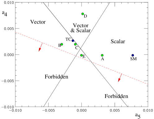
Figure 1: Map of the parameter space as determined by the Padé protocol [10]. The small triangle in the centre is the region of no resonances and the region below the dotted line is forbidden. Also shown are the points corresponding to the various scenarios considered in the text.

In the Padé approach we can solve this equation to obtain the corresponding masses and widths [10]. For scalar resonances:

$$m_{S}^{2}=\frac{{4v^{2}}}{\frac{{16}}{3}(11a_{5}(\mu)+7a_{4}(\mu))+\frac{{1}}{16\pi^{2}}\left(\frac{{101-50\log(m_{S}^{2}/\mu^{2})}}{9}\right)}$$ (22)

and

$$\Gamma_{S}=\frac{{m_{S}^{3}}}{16\pi v^{2}}.$$

For vector resonances:

$$m_{V}^{2}=\frac{{v^{2}}}{4(a_{4}(\mu)-2a_{5}(\mu))+\frac{{1}}{16\pi^{2}}\frac{{1}}{9}}$$ (23)

and

$$\Gamma_{V}=\frac{{m_{V}^{3}}}{96\pi v^{2}}.$$

There are no resonances in the isotensor channel, i.e. from $t_{20}$. There is however a region of parameter space where the phase shift passes through $-\pi/2$. This would violate causality and so we are forced to forbid such regions of parameter space. It occurs when

$$\frac{{32}}{3}(a_{5}(\mu)+2a_{4}(\mu))+\frac{1}{16\pi^{2}}\left(\frac{273}{54}-\frac{20}{9}\log\frac{s}{\mu^{2}}\right)<0.$$ (24)

A map of the $a_{4}-a_{5}$ parameter space showing the corresponding resonance structure is presented in Figure 1. We fix $\mu=1$ TeV and, using equations (22) and (23), we define the regions to contain a resonance of the specified type with mass below 2 TeV. The blue points labelled TC and SM correspond to the naive $N_{TC}=3$ technicolor (TC) and 1 TeV Standard Model Higgs (SM) models.

The $N/D$ protocol

This provides our alternative to the Padé protocol. This method ensures that the amplitude has improved analytic properties in addition to satisfying partial wave unitarity and matching the one-loop EWChL calculation. The right-hand cut is placed wholly into the denominator function, $D$, while the left-hand cut is encapsulated in the numerator function, $N$, i.e. analyticity and unitarity demand the following relations [22, 23, 24]:

$${\rm Im}(t_{IJ}(s)^{-1})=-1\qquad s>0$$ (25)

$${\rm Im}\,D(s)=0\qquad s<0$$ (26)

$${\rm Im}\,N(s)=D\,{\rm Im}\,t_{IJ}(s)\qquad s<0$$ (27)

$${\rm Im}\,N(s)=0\qquad s>0$$ (28)

where

$$t_{IJ}(s)=\frac{N(s)}{D(s)}.$$ (29)

Following Oller, we define the following function to contain the right-hand cut at $s=M^{2}$ [23]:

$$g(s)=\frac{1}{\pi}\log\left(-\frac{s}{M^{2}}\right)$$ (30)

where $M$ is an unknown parameter. The $N/D$ unitarised partial wave amplitude is then written

$$t_{IJ}(s)=\frac{X_{IJ}(s)}{1+g(s)X_{IJ}(s)}$$ (31)

where

$$X_{IJ}(s)=t^{(2)}_{IJ}(s)+t^{(4)}_{IJ}(s)+g(s)(t^{(2)}_{IJ}(s))^{2}.$$ (32)

The amplitude thus defined has been constructed so as to satisfy (25) and (28) identically whilst (26) and (27) are satisfied to one-loop in chiral perturbation theory. Note that the contribution to ${\rm Im}\,D(s)$ for $s<0$ is beyond the one-loop approximation.

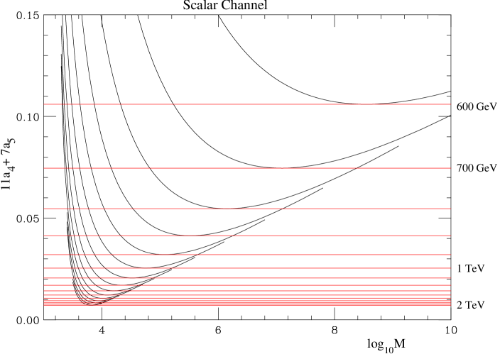
Figure 2: Contours of constant scalar resonance mass in steps of 100 GeV. The horizontal lines are obtained using the Padé protocol and the curved lines are obtained using the N/D method which depends upon the parameter $M$.

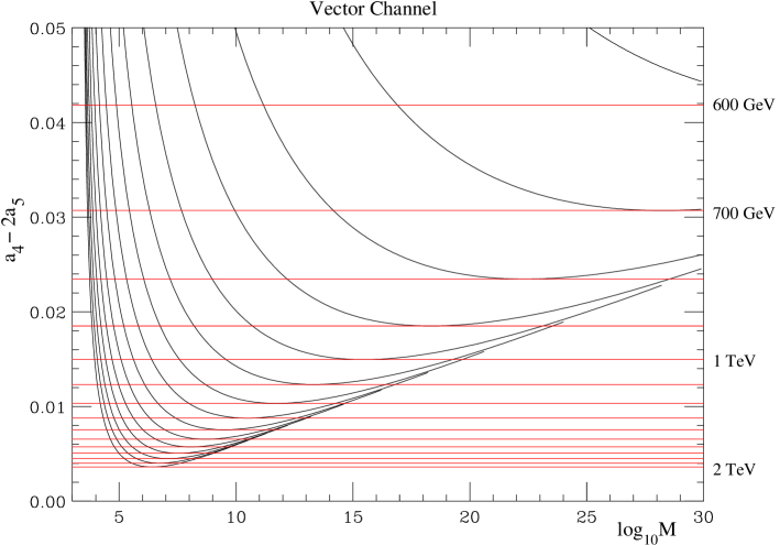
Figure 3: Contours of constant vector resonance mass in steps of 100 GeV. The horizontal lines are obtained using the Padé protocol and the curved lines are obtained using the N/D method which depends upon the parameter $M$.

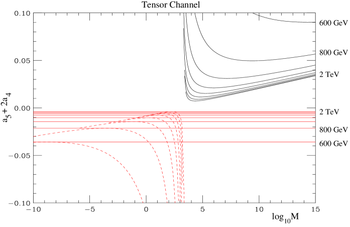
Figure 4: Contours of constant isotensor resonance mass in steps of 100 GeV. The curved lines are obtained using the N/D method which depends upon the parameter $M$. The horizontal lines and dotted curves populate the unphysical region of parameter space, see the discussion in the text.

In Figures 2 to 4 we show curves of constant resonance mass, varying from 600 GeV to 2 TeV in steps of 100 GeV, as a function of the appropriate combination of $a_{4}(1$ TeV), $a_{5}(1$ TeV), and $M$. The horizontal lines obtained using the Padé protocol are tangent to the corresponding N/D contours. Over large regions of parameter space, the two protocols yield similar results. However, the N/D method predicts a larger region without resonances, indeed for $M$ below around 1 TeV there are no resonances at all. Referring back to Figure 1, we see that as $M$ increases the lines which define the scalar and vector regions move slowly outwards. From Figure 4 we see that for $M$ above $\sim 1$ TeV the region excluded in the Padé protocol is not excluded in the N/D protocol leading instead to a region without any resonances. For $M$ below $\sim 1$ TeV, there is a region excluded by N/D unitarisation (for the same reason as in the earlier Padé case). The line delineating the forbidden region in Figure 1 thus moves slowly downwards as $M$ decreases. Note that we do not know the natural value for $M$, e.g. it can be much smaller than 1 TeV. Finally, we note from Figure 4 that the N/D method does allow for the existence of doubly charged resonances.

4 Parton Level Predictions for the LHC

Scenario	$a_{4}$(1 TeV)	$a_{5}$(1 TeV)
A	0.0	0.003
B	0.002	-0.003
C	0.002	-0.001
D	0.008	0
E	0	0

Table 1: Parameters for the five scenarios which we consider.

In this section the parton level predictions for the process $pp\to W^{+}W^{-}jj+X$ at 14 TeV centre-of-mass energy are presented for the 5 different choices of $a_{4}$ and $a_{5}$ shown in Table 1. In the Padé approach these choices produce a 1 TeV scalar (scenario A), a 1 TeV vector (scenario B), a 1.9 TeV vector (scenario C), a 800 GeV scalar and a 1.4 TeV vector (scenario D), and a scenario with no resonances (scenario E). The green points labelled A-E on Figure 1 correspond to the 5 scenarios we consider. Throughout this paper the CTEQ4L [25] parton density functions as implemented in PDFLIB [26] are used, evaluated at the $WW$ centre-of-mass energy $(M_{WW})$. The renormalisation scale is fixed to 1 TeV. The differential cross-section $d\sigma/dM_{WW}$ for each of scenarios A-E are shown in Figures 5-9. We compare the Padé protocol with results using the N/D protocol for three different values of the mass parameter $M$.

Figure 5: Parton level cross-section for Scenario A. We compare the Padé result (solid line) with the N/D results for $M=10^{3}$ GeV(dashed line), $M=10^{4}$ GeV (dashed-dotted line) and $M=10^{5}$ GeV (dotted line).

Figure 6: Parton level cross-section for Scenario B. We compare the Padé result with the N/D results as in Figure 5.

Figure 7: Parton level cross-section for Scenario C. We compare the Padé result with the N/D results as in Figure 5.

Figure 8: Parton level cross-section for Scenario D. We compare the Padé result with the N/D results as in Figure 5.

Figure 9: Parton level cross-section for Scenario E. We compare the Padé result with the N/D results as in Figure 5.

Note that, for values of $M$ below around 10 TeV there are no resonances at all in the N/D scenario. This is in accord with expectations based on Figures 2 to 4. Also, if $M$ becomes too large then it leads to unusual behaviour of the amplitudes due to the dominance of the $g(s)$ term which suppresses the amplitudes away from the region of resonances and can produce zeros in the individual partial wave amplitudes. The tail in the dotted line shown in Figure 9 is a consequence of such behaviour. Just discernable in Figure 8 is an isospin 2 scalar resonance just below 1.5 TeV in the N/D dotted curve.

5 Monte Carlo Simulations

We have modified the Pythia Monte Carlo generator [15] to include the EWChL approach using both Padé and N/D protocols. Signal samples containing the $W^{\pm}W^{\pm}$ final state (including all charge combinations) are generated using Pythia 6.146 with the Padé unitarisation scheme. As a cross check, a sample with a 1 TeV Higgs was also generated using Herwig 6.1 [27].

Figure 10: Typical diagrams for signal and background processes: (a) signal; (b) $W+$jets; (c) $t{}\bar{t}$

The dominant backgrounds are QCD $t\bar{t}$ production and radiative $W+$jets, as illustrated in Figure 10. These processes are implemented in the Pythia 6.146 and Herwig 6.1 generators. To improve generation efficiency the minimum $p_{T}$ of the hard scatter is set to 250 GeV for the $W+$ jets sample and to 300 GeV for the $t\bar{t}$ sample [6]. In addition to the hard subprocesses, the effects of the “underlying event” are simulated in both signal and background. Our default model in Pythia [28] is obtained by setting a fixed minimum $p_{T}$ cut off of $p_{T}^{min}=3$ GeV for secondary scatters. The default energy dependence of this cut-off has been explicitly turned off. No pile-up from multiple $pp$ interactions is included. Other models, in both Herwig and Pythia, are discussed in Section 8, along with their effects. The leading order cross-sections are used to obtain rates and there is therefore a rather large degree of uncertainty, particularly in $t\bar{t}$ production, which is a pure QCD, dominantly gluon induced, process. NLO calculations [29] suggest K-factors of order two are appropriate; the final word would come from measurements at the LHC itself.

6 Extracting the Signal

To identify semileptonic decays, we select first on the leptonically decaying $W$ (electron/muon and missing transverse energy), then on the hadronically decaying $W$ (jet invariant mass, rapidity and transverse energy) and finally on the event environment (tagging jets at high rapidities, vetoing on central minijet activity). In all cases we have used only particles within a rapidity region of $|\eta|<4.5$ to approximate the acceptance of a general purpose detector at the LHC. For clarity, we show just one signal sample as an example. The 1 TeV scalar resonance (scenario A) is chosen, since this has the lowest average $M_{WW}$ and therefore has a shape closest to that of the backgrounds. The other scenarios, while in general very like this sample, have a harder spectrum in the transverse momentum variables. The analysis follows the 1 TeV Higgs study of [6] quite closely for many cuts. However, we differ in the identification of hadronically decaying $W$ bosons via the subjet method, in the top quark veto, in the cut on the transverse momentum of the hard system, and in details of other cuts; all of which are described below.

6.1 Leptonic Variables

Figure 11 shows (a) the transverse momentum and (b) rapidity of the highest transverse momentum charged lepton for signal and background processes. The $W+$jets background is very similar to the signal in these distributions. Leptons from the $t\overline{t}$ background are slightly softer and more central. Figure 11(c) shows the missing transverse momentum. Again, the $t\overline{t}$ background is slightly softer than the other two samples.

All leptons in an event are then combined one-by-one to give, if possible, a reconstructed $W$ boson (to within a twofold ambiguity due to the unknown $z$ component of the neutrino momentum). The transverse momentum of all these $W$ candidates is shown in Figure 11(d). The signal has a harder distribution than both backgrounds. A selection cut is applied at 320 GeV on this distribution and in the case that more than one candidate is present, that with the highest transverse momentum is used.

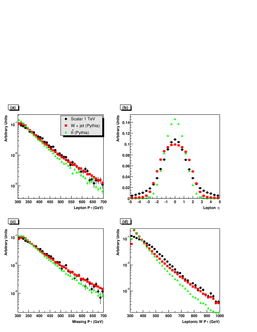
Figure 11: Leptonic variables for signals and background (a) transverse momentum of the highest $p_{T}$ charged lepton ($e$ or $\mu$), (b) pseudorapidity of the same lepton, (c) missing transverse momentum and (d) the $p_{T}$ of the $W$ candidate constructed from the lepton and the assumed neutrino. The area under the histograms is set to one to allow comparison of the shapes. A trigger cut at 80 GeV in the $p_{T}$ of the highest $p_{T}$ jet and at 40 GeV in the highest $p_{T}$ charge lepton is applied before making the plots, as well as a realistic rapidity acceptance.

6.2 The Hadronic $W$ Decay

Figure 12(a) shows the transverse momentum and (b) the pseudorapidity ($\eta$) of the highest transverse momentum jet in the remaining signal and background samples. Jet finding is performed with the inclusive $k_{T}$ algorithm [14], and the $E$ recombination scheme is used throughout. To reconstruct the $W$ mass, the highest transverse momentum jet within the region $|\eta|<4$ is selected. In the $E$ recombination scheme the candidate $W$ mass, $M_{J}$ is then the invariant mass of this jet. Figure 12(c) shows this distribution, with $W$ mass peaks visible in the signal and in the $t\overline{t}$ sample, and a top mass peak also visible in the $t\overline{t}$ events. Cuts are applied at $p_{T}>320$ GeV, and $70$ GeV$<M_{J}<90$ GeV. The results (after this cut and the leptonic cuts) are shown in the second and third rows of Table 2.

The jet is next forced to decompose into two subjets. The possibility of using subjets to reconstruct massive particles decaying to hadrons has been discussed previously [30]. In this analysis we develop a new technique. The extra pieces of information gained from the subjet decomposition are the $y$ cut at which the subjets are defined and the four-vectors of the subjets. For a genuine $W$ decay the expectation is that the scale at which the jet is resolved into subjets (i.e. $yp_{T}^{2}$) will be ${\cal{O}}(M_{W}^{2})$. The distribution of $\log(p_{T}\sqrt{y})$ is shown in Figure 12(d). The scale of the splitting is indeed high in the signal and softer in the $W+$ jets background, where the hadronic $W$ is in general a QCD jet rather than a genuine second $W$. A cut is applied at $1.6<\log(p_{T}\sqrt{y})<2.0$. The effect of this cut is shown in the fourth row of the table. Whilst this is a powerful cut for reducing the $W+$ jets background, the effect on the $t\overline{t}$ background, which more often contains two real $W$ bosons, is less marked.

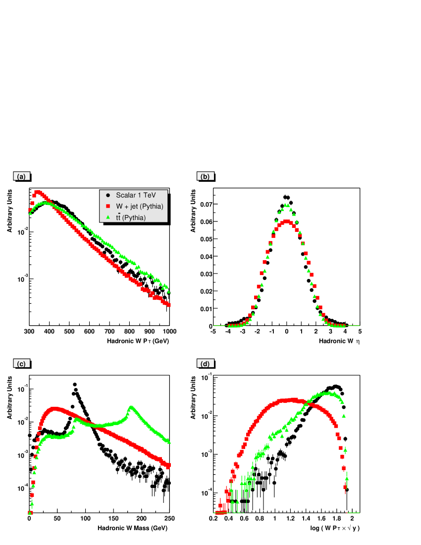
Figure 12: Kinematic variables for the hadronically decaying $W$ candidate. (a) $p_{T}$, (b) $\eta$, (c) Invariant mass (d) $p_{T}\sqrt{y}$ . The area under the histograms is set to unity to allow comparison of the shapes.

6.3 The Hadronic Environment

To further reduce backgrounds, cuts must be applied to characteristics of the event other than those directly related to the decaying $W$ bosons.

Top quark veto

In the remaining $t\overline{t}$ events containing a genuine leptonic $W$, the $W$ will combine with a jet other than the hadronic $W$ candidate to give a mass close to the top mass. This mass distribution for the leptonic $W$ candidate combined separately with each such jet in the event is shown in Figure 13(a). The top peak is clearly visible in the $t\overline{t}$ sample. Any event with a mass in the region 130 GeV $<M_{wj}<$ 240 GeV is rejected. A similar distribution (not shown) is obtained by combining the hadronic $W$ candidate with other jets in the event, and the same cut is applied. In combination these cuts are decribed as a “top quark veto”, and their effect is shown row five of Table 2.

Tag jets

In the $WW$ scattering process the bosons are radiated from quarks in the initial state (see Figure 10(a)). The quark from which the boson is radiated will give a jet at high rapidity (i.e. close to the direction of the hadron from which it emerged). These jets are not in general present in the background processes and demanding their presence is therefore a powerful tag of the signal [13]. In this analysis we define a “tag jet” as follows. The event is divided into three regions of rapidity: “forward”, i.e. forward of the most forward $W$; “backward”, i.e. backward of the most backward $W$; and “central”, i.e. the remaining region, which includes both $W$ candidates. A forward (backward) tag jet is defined as the highest transverse energy jet in the forward (backward) region. In Figure 13(b) the rapidity distribution of the tag jets with $p_{T}>20$ GeV is shown. Signal events display an enhancement at high $|\eta|$ and a suppression at low $|\eta|$, in dramatic contrast to the background processes, where most jets are central. For an event to be retained it must have a tag jet in both the forward and backward regions satisfying $p_{T}>20$ GeV, $E>300$ GeV and $4.5>|\eta|>2$. The result of imposing this cut is shown in row six of Table 2. The background is reduced by a factor of around fifty, at the cost of a loss less than two thirds of the signal.

Hard $p_{T}$

Figure 13(c) shows the $p_{T}$ distribution for the “hard scattering” system comprising the two tags jets and the two $W$ candidates. For events surviving the cuts so far, the background events have a harder spectrum than the signal, since in the signal events this system is the complete result of a scattering between colinear partons, whereas in the backgrounds extra jets from hard QCD radiation may be picked up and/or missed. An upper cut is applied at 50 GeV, and the results are shown in row seven of Table 2.

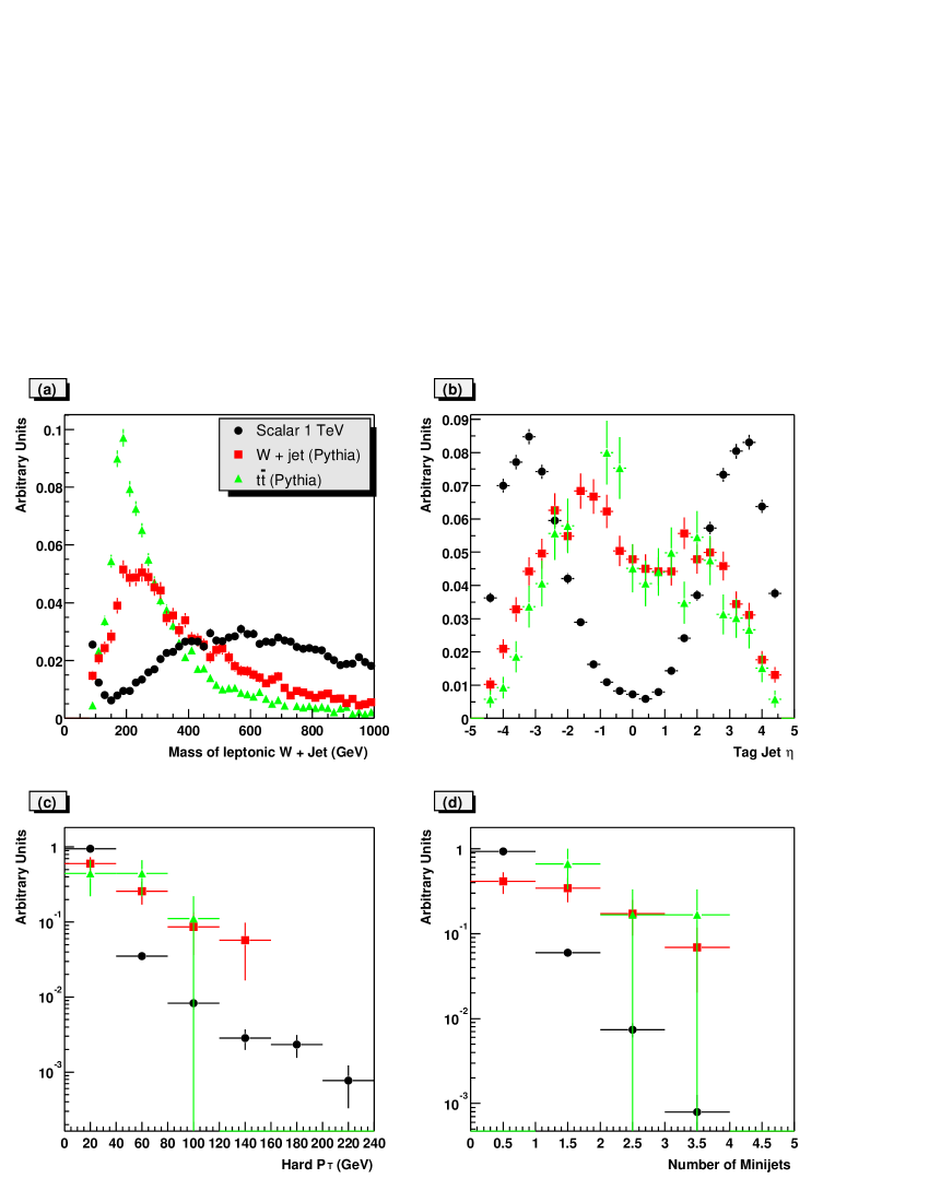
Figure 13: (a) The mass distribution for the leptonic W candidate combined seperately with all other jets in the event other than the hadronic $W$ candidate. (b) The rapidity distribution for tag jets (see text). (c) The transverse momentum distribution for the $WW+$ tag jets system. (d) The number of minijets (see text).

Minijet Veto

Finally, a cut which has been employed before in similar analyses [5, 11, 12] exploits the fact that for signal events no colour is exchanged between the quarks which radiate the $W$ bosons and the jets which are produced by the hadronically decaying $W$. This leads to a suppression of QCD radiation in the central region in the signal with respect to the background. However, significant activity is expected in all classes of event due to remnant-remnant interactions (“underlying event”). This activity can produce additional (mini)jets, and so it is important to choose a cut on additional jet activity which is robust against the large uncertainties in current understanding of the underlying event at the LHC. In this analysis minijets are defined as all jets apart from the hadronic $W$ candidate with $|\eta|<2$. Events are vetoed if the number of minijets with $p_{T}>15$ GeV is greater than one. The distribution of the number of jets satisfying these demands is shown in Figure 13(d). The result of applying this cut is shown in row eight of Table 2. This cut is discussed further in Section 8.

7 Analysing the signal

7.1 Efficiency and Event Numbers

Having applied the cuts described in the previous section, the $WW$ mass distribution obtained is shown in Figure 14(a) and (b) for all five signal samples discussed above. The resolution obtained in this variable is around 10 GeV, before any detector smearing. The efficiency is shown as a function of the true $WW$ mass in (e). It rises from zero to 6% between 500 GeV and 1.5 TeV, and is flat above this value. This efficiency includes the branching ratio for semileptonic $W$ decays of around 15% . Excluding the branching ratio, the efficiency is around 40%.

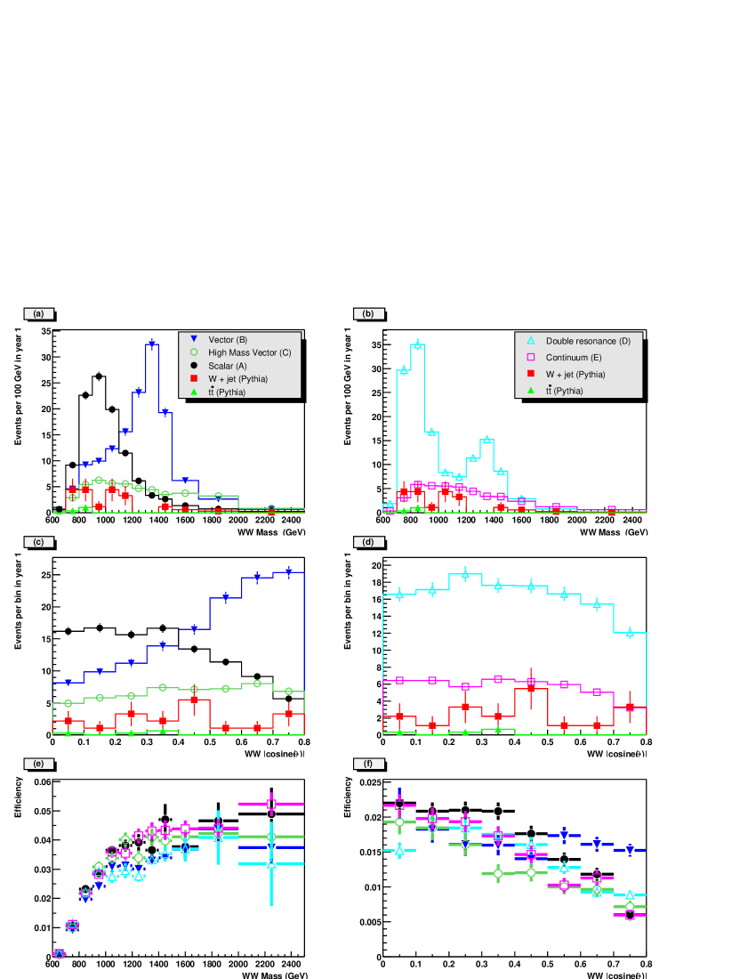
Figure 14: (a,b) Distribution of the reconstructed $WW$ mass for signals and backgrounds separately. (c,d) Distribution of $|\cos\theta^{*}|$, the absolute value of the cosine of the centre-of-mass scattering angle for signals and backgrounds seperately. (e) Efficiency for signal events as a function of the true $M_{WW}$ and (f) $|\cos\theta^{*}|$. The errors reflect the statistics which would be obtained after approximately one year of running at the LHC, i.e. 100 fb^-1.

A key variable for distinguishing between scalar and vector resonances is the angular distribution of the scattered $W$ pair in the $WW$ centre-of-mass system. In Figure 14(c) and (d) the distribution of $|\cos\theta^{*}|$ is shown, where $\theta^{*}$ is the angle between the scattered $W$ and the incoming $W$ direction, in the $WW$ centre-of-mass frame. In (f) the efficiency is shown. The efficiency is very dependent on the mass distribution, since for the same transverse momentum, high scattering angles have high mass. This means that the transverse momentum cuts bias this distribution. However, this bias is well understood and could be corrected for in a final measurement using a two-dimensional correction in mass and angle regardless of the input distribution.

7.2 Simulated Measurement

If it is assumed that the backgrounds can be well constrained from developments in theory, measurements at the Tevatron and HERA over the next few years, and measurements at the LHC in other kinematic regions, then the statistical error on an extraction of the $M_{WW}$ and $|\cos\theta^{*}|$ distributions can be estimated by adding the statistical errors on the signal and background distributions in quadrature. Under this assumption, a simulation of an expected measurement of the differential cross-section $d\sigma/dM_{WW}$ after 100 fb^-1 of LHC luminosity is shown in Figure 15(a), (c) and (e). The scenarios containing resonances are distinguishable above the background, and are also distinguishable from each other due to their different resonant masses. In Figure 15(c) the double resonance sample (D) is shown, with two peaks clearly measured. Also shown (in all three figures) is the continuum model (E).

The expected measurement of the differential cross-section $d\sigma/d|\cos\vartheta^{*}|$ after 100 fb^-1 of LHC luminosity is shown in Figure 15(b),(d) and (f) for $M_{WW}>750$ GeV. The intermediate mass vector and scalar resonances have the expected behaviour, with the vector rising towards high $|\cos\theta^{*}|$ and the scalar being flat. In Figure 15(d) the distribution for the double resonance model is shown in two mass bins: $750<M_{WW}<1200$ GeV and $M_{WW}>1200$ GeV. With the high statistics generated (corresponding to a very high integrated luminosity), the lower mass resonance can be seen to be a scalar whilst the higher mass is a vector. However, within the simulated errors the measurement of the spin of the lower mass resonance would be marginal.

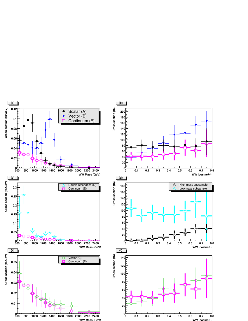
Figure 15: Measurement expectation after 100 fb^-1 of LHC luminosity at 14 TeV cm energy. (a,c,e) $d\sigma/dM_{WW}$ and (b,d,f) $d\sigma/d|\cos\theta^{*}|$. (d) shows $d\sigma/d|\cos\theta^{*}|$ for the high and low mass subsamples for the double resonance model, separated by a cut at 1200 GeV.

Cuts	Efficiency	Signal	$t\overline{t}$	$W+$Jets	Sig/B
		$\sigma$ (fb)	$\sigma$ (fb)	$\sigma$ (fb)
Generated	A:100%	72	Pythia		$8.7\times 10^{-4}$
	B:100%	104	18,000	65,000	$1.3\times 10^{-3}$
	C:100%	44	Herwig		$5.3\times 10^{-4}$
	D:100%	113	14,000	53,000	$1.4\times 10^{-3}$
	E:100%	47			$5.0\times 10^{-4}$
$p_{T}$ (Lep. $W$ )$>320$ GeV	A:11%	8.2	Pythia		$1.5\times 10^{-3}$
and	B:11%	11	910	4400	$2.1\times 10^{-3}$
$p_{T}$ (Had. $W$) $>320$ GeV	C:10%	4.4	Herwig		$8.3\times 10^{-4}$
	D:10%	11	750	3600	$2.1\times 10^{-3}$
	E:10%	4.7			$8.8\times 10^{-4}$
70 GeV $<M$(Had. $W$ )	A:6.7%	4.8	Pythia		$6.3\times 10^{-3}$
$<90$ GeV	B:6.2%	6.4	56	700	$8.4\times 10^{-3}$
	C:5.8%	2.6	Herwig		$3.4\times 10^{-3}$
	D:5.6%	6.3	52	480	$8.3\times 10^{-3}$
	E:5.8%	2.7			$3.6\times 10^{-3}$
$1.6<\log(p_{T}\times\sqrt{y}$ $)<2.0$	A:4.7%	3.4	Pythia		$3.2\times 10^{-2}$
	B:4.4%	4.5	28	78	$4.3\times 10^{-2}$
	C:4.1%	1.8	Herwig		$1.7\times 10^{-2}$
	D:4.0%	4.5	27	66	$4.3\times 10^{-2}$
	E:4.1%	1.9			$1.8\times 10^{-2}$
Top quark veto	A:4.3%	3.1	Pythia		$5.6\times 10^{-2}$
(see text)	B:4.0%	4.2	3.2	52	$7.5\times 10^{-2}$
	C:3.8%	1.7	Herwig		$3.0\times 10^{-2}$
	D:3.6%	4.1	3.4	43	$7.3\times 10^{-2}$
	E:3.8%	1.8			$3.2\times 10^{-2}$
Tag jets	A:1.6%	1.1	Pythia		2.7
$p_{T}>20$ GeV, $E>300$ GeV	B:1.5%	1.6	0.030	0.38	3.8
(see text)	C:1.4%	0.63	Herwig		1.5
	D:1.3%	1.5	0.082	0.42	3.6
	E:1.4%	0.67			1.6
Hard $p_{T}<50$ GeV	A:1.5%	1.1	Pythia		3.2
	B:1.5%	1.5	0.020	0.32	4.5
	C:1.4%	0.61	Herwig		1.8
	D:1.3%	1.4	0.048	0.37	4.3
	E:1.4%	0.65			1.9
Minijet veto	A:1.5%	1.1	Pythia		4.3
$p_{T}>15$ GeV, see text	B:1.5%	1.5	0.013	0.24	6.0
	C:1.4%	0.61	Herwig		2.4
	D:1.3%	1.4	0.048	0.36	5.6
	E:1.4%	0.65			2.6

Table 2: The effect of cuts on the signal and background samples. A: 1 TeV scalar, B: 1.4 TeV Vector, C: 2 TeV Vector, D: Double Resonance and E: Continuum.

8 The Underlying Event

One of the more uncertain aspects of the analysis is the understanding of the so-called “underlying event”. This is defined here as particle and energy flow in the event associated with the same proton-proton interaction but incoherent with the $W$ production process. Hence we explicitly exclude from our definition the effects of multiple $pp$ interactions in the same bunch crossing, any detector effects such as those associated with noise or pile-up, and hard QCD radiation associated directly with the hard scatter. The first two of these are not simulated here and controlling and understanding them requires detailed experimental work. The third is simulated to leading-logarithmic accuracy in both Pythia and Herwig. While this simulation should and probably will be improved in the future, for now it is considered adequate.

The remaining activity can be characterised as interactions between the proton remnant systems. It is important because it is largely independent of the hard scattering process, and therefore contributes to minijet activity in both signal and background, degrading the effectiveness of the minijet veto. In addition, underlying event activity contributes to the observed $W$ width and the position of the mass peaks in a highly model-dependent way.

In Figure 16(a) and (b) the jet mass distribution and the $\log(p_{T}\sqrt{y})$ are shown again (as in Figure 12(c) and (d)) for the signal events (1 TeV resonance, sample A) using our default underlying event model. In addition, several other underlying event models are shown. In Pythia, we turn off multiparton interactions (sample A1), and turn on the default model (sample A2) which has a $p_{T}^{min}$ of 2.89 GeV at LHC energies. Also shown are three samples of 1 TeV Higgs events generated using herwig. These have no underlying event (sample A3), soft underlying event (sample A4) and multiparton interactions generated with fixed $p_{T}^{min}=3.0$ GeV (sample A5)[31]. The width of the $W$ mass peak is much greater in general for those samples which include an underlying event. Whilst the pythia multiparton interaction models and the Herwig soft underlying event are fairly consistent with each other, the Herwig multiparton interaction model gives a very different distribution. However, the $\log(p_{T}\sqrt{y})$ is similar for all models, implying that this cut should be robust against such uncertainties.

For the same samples, the minijet $p_{T}$ distribution and the number of minjets passing the 15 GeV cut, which we introduced in the analysis of Section 6.3, are shown in Figure 16(c) and (d), with absolute normalisation. In contrast to the $W$ mass distribution, in these distributions the Herwig multiparton interaction model is close to the pythia multiparton models, whereas the soft underlying event model is closer to the models without underlying event. The $p_{T}$ distribution is very steeply falling, and is sensitive to the underlying event below around 20 GeV. Thus, there is sensitivity in the number of jets at 15 GeV, and this would become worse for lower choices of cut. Lowering the cut further without introducing large uncertainties requires a better knowledge of the underlying event than is currently available.

If the no underlying event model is used in pythia (sample A1), the signal/background for the scenario A is 8.0. However, for all other cases (models A, A2-A5) the ratio is between 2.5 and 4.0. Data from the Tevatron and photoproduction at HERA (see for example [32] and references therein), strongly disfavour models without underlying event (A1, A3) and are generally more consistent with the other models considered here (though none provides a perfect description). However, further work is needed on constraining these models to improve confidence in the extrapolation to the LHC. At present a systematic error of 40-50% would have to be assigned to the measurement from this source alone.

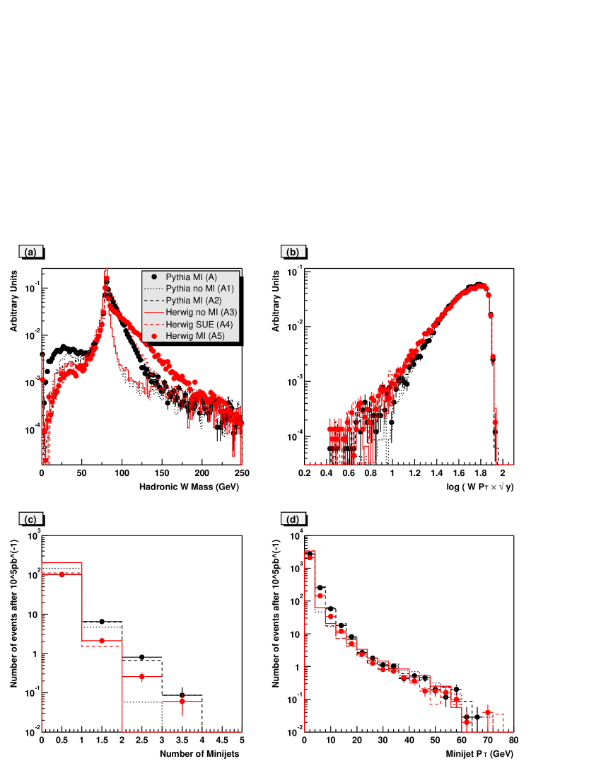
Figure 16: The effect of the underlying event. (a) Hadronic $W$ mass, (b) $p_{T}\sqrt{y}$ , (c) Number of minijets and (d) the $p_{T}$ distribution of the minijets.

9 Summary and Conclusions

A major goal of the LHC is to extract the $WW\rightarrow WW$ cross-section as accurately as possible to the highest centre-of-mass energies in order to shed light on the nature of electroweak symmetry breaking. We have performed a study of the $WW\to WW$ scattering cross-section in the scenario that there is no new physics below the TeV scale using the formalism of the Electroweak Chiral Lagrangian extended by the imposition of unitarity constraints. Two different unitarisation protocols are used: Padé and N/D. These protocols determine the behaviour of the scattering cross-section into the TeV regime and they typically predict the emergence of new vector and/or scalar resonances. We have performed a detailed comparison of these two unitarisation methods.

We have implemented the physics of the unitarised Electroweak Chiral Lagrangian in a realistic general-purpose Monte Carlo (Pythia). The semi-leptonic decay mode of the final state $W$ pair has been studied at the final state particle level with detector acceptance cuts but no smearing. We have considered five different physics scenarios which are representative of the different types of physics which we might reasonably expect at the LHC. The principal backgrounds come from $W+$ jet and $t\overline{t}$ production, and we consider these backgrounds using both the pythia and herwig Monte Carlos. A new method for identifying hadronically decaying $W$ bosons is introduced which we expect to be useful more generally in the identification of hadronically decaying massive particles which have energy large compared to their mass. Other new features include a top quark veto and a cut on the transverse momentum of the hard subsystem. In addition, the established tag jet and minijet veto cuts are applied. The results are cross-checked with Herwig using a simulation of a 1 TeV Higgs boson for the signal. The effect of uncertainties in the underlying event leads to a model dependent systematic error of 40-50%. New data from Tevatron and HERA should help to reduce this before the LHC turns on.

The results compare very well with previous Higgs search studies in the semi-leptonic channel. Over a wide range of parameter space signal/background ratios of greater than unity can be obtained, and the cross-section can be measured differentially in the $WW$ centre-of-mass energy within one year of high luminosity LHC running (100 fb^-1). Vector and scalar resonances up to around 1.5 TeV may well be observable, and their spins measureable. Detailing the exact regions of sensitivity, as well as verifying the improvements in signal/background arising from the new cuts, requires a more detailed simulation of the LHC general purpose detectors.

Acknowledgements

Thanks to Anahita New, José Oller and Graham Shaw for their valuable contributions. This work was supported by the UK Particle Physics and Astronomy Research Council (PPARC).

References

- [1] LEP Electroweak Working Group, CERN-EP/2001-021 and references therein.
- [2] R. Sekhar Chivukula and N. Evans, Phys. Lett. B464 (1999) 244; R. Barbieri and A. Strumia, Phys. Lett. B462 (1999) 144; C. Kolda and H. Murayama, JHEP 0007 (2000) 035; M.E. Peskin and J.D. Wells, Phys. Rev. D64 (2001) 115002; J.R. Forshaw, D.A. Ross and B.E. White, JHEP 0110 (2001) 007.
- [3] J. A. Bagger, A. Falk and M. Swartz, Phys. Rev. Lett. 84 (2000) 1385.
- [4] T. Applequist and C. Bernard, Phys. Rev. D22 (1980) 200; A. Longhitano, Phys. Rev. D22 (1980) 1166; A. Longhitano, Nucl. Phys. B188 (1981) 118.
- [5] ATLAS Collaboration, Technical Proposal, CERN/LHCC/94-13; CMS Collaboration, Technical Proposal, CERN/LHCC/94-38.
- [6] ATLAS Collaboration, Detector and Physics Performance Technical Design Report, CERN/LHCC/99-15.
- [7] M.Golden, T.Han and G.Valencia, in “Electroweak Symmetry Breaking and New Physics at the TeV Scale”, ed. T.L. Barklow, hep-ph/9511206.
- [8] T.L. Barklow et al, Working Group Summary Report from the 1996 DPF/DPB Summer Study, New Directions for High Energy Physics, Snowmass, Colorado, hep-ph/9704217.
- [9] J. Bagger et al, Phys. Rev. D52 (1995) 3878.
- [10] A. Dobado, M.J. Herrero, J.R. Peláez and E. Ruiz Morales, Phys. Rev. D62 (2000) 055011.
- [11] K. Iordanidis & D. Zeppenfeld, Phys. Rev D57 (1998) 3072; R. Rainwater and D. Zeppenfeld, Phys. Rev. D60 (1999) 113004; erratum ibid D61 (2000) 099901.
- [12] V. Barger et al, Phys. Rev. D44 (1991) 1426; ibid D44 (1991) 2701.
- [13] R.H. Cahn, S.D. Ellis and W.J. Stirling, Phys. Rev. D35 (1987) 1626; V. Barger, T. Han and R.J.N. Phillips, Phys. Rev. D37 (1988) 2005; R. Kleiss and W.J. Stirling, Phys. Lett. B200 (1988) 193.
- [14] S. Catani et al, Nucl. Phys. B406 (1993) 187.
- [15] T. Sjöstrand, Comp. Phys. Comm. 82 (1994) 74.
- [16] A.S. Belyaev et al, Phys. Rev. D59 (1999) 015022.
- [17] J.M. Cornwall, D.N. Levin and G. Tiktopoulos, Phys. Rev. D10 (1974) 1145; B.W. Lee, C. Quigg and H. Thacker, Phys. Rev. D16 (1977) 1519; M.S. Chanowitz and M.K. Gaillard, Nucl. Phys. B261 (1985) 379.
- [18] A. Dobado, M.J. Herrero and T.N. Truong, Phys. Lett. B235 (1990) 129; A. Dobado, M.J. Herrero and J. Terrón, Z. Phys. C50 (1991) 205; ibid. C50 (1991) 465.
- [19] A. Dobado and J.R. Peláez, Phys. Rev. D47 (1993) 4883; ibid. D56 (1997) 3057; J.A. Oller, E. Oset and J.R. Peláez, Phys. Rev. Lett. 80 (1998) 3452; Phys. Rev. D59 (1999) 074001; ibid. erratum D60 (1999) 099906; F. Guerrero and J.A. Oller, Nucl. Phys. B537 (1999) 459.
- [20] S. Dawson, Nucl. Phys. B249 (1985) 42.
- [21] J.R.Peláez, Phys. Rev. D55 (1997) 4193.
- [22] B.R. Martin, D. Morgan and G. Shaw, “Pion-Pion Interactions in Particle Physics”, Academic Press.
- [23] J.A. Oller, Phys. Lett. B477 (2000) 187.
- [24] K. Hikasa and K. Igi, Phys. Rev. D48 (1993) 3055; S.R. Beane and C.B. Chiu, hep-ph/9303254.
- [25] H.L.Lai et al, Phys. Rev. D55 (1997) 1280.
- [26] H.Plothow-Besch, Comp. Phys. Comm. 75 (1993) 396.
- [27] G.Marchesini et al., Comp. Phys. Comm. 67 (1992) 465; hep-ph/9912396.
- [28] T. Sjöstrand and M. van Zijl, Phys. Rev. D36 (1987) 2019.
- [29] R. Bonciani et al., Nucl. Phys. B529 (1998) 424.
- [30] M.H. Seymour, Z. Phys. C62 (1994) 127.
- [31] J. M. Butterworth, J. R. Forshaw and M. H. Seymour, Z. Phys. C72 (1996) 637.
- [32] CDF Collaboration, D. Acosta et al, FERMILAB-PUB-01-345-E, Oct 2001, submitted to Phys. Rev. D; J. M. Butterworth and R. J. Taylor, Proceedings of Photon 99, Nucl. Phys Proc. Suppl., 82, (2000) 112, http://www.hep.ucl.ac.uk/JetWeb; ZEUS Collaboration, J. Breitweg et al, E. Phys. J. C1 (1998) 109; H1 Collaboration, C. Adloff et al, Phys. Lett. B483 (2000) 36.