Current-carrying cosmic string loops 3D simulation:
towards a reduction of the vorton excess problem.

Abstract

The dynamical evolution of superconducting cosmic string loops with specific equations of state describing timelike and spacelike currents is studied numerically. This analysis extends previous work in two directions: first it shows results coming from a fully three dimensional simulation (as opposed to the two dimensional case already studied), and it now includes fermionic as well as bosonic currents. We confirm that in the case of bosonic currents, shocks are formed in the magnetic regime and kinks in the electric regime. For a loop endowed with a fermionic current with zero-mode carriers, we show that only kinks form along the string worldsheet, therefore making these loops slightly more stable against charge carrier radiation, the likely outcome of either shocks or kinks. All these combined effects tend to reduce the number density of stable loops and contribute to ease the vorton excess problem. As a bonus, these effects also may provide new ways of producing high energy cosmic rays.

I Introduction

Superconducting cosmic strings are topological defects kibble that may be formed at a phase transition in the early universe witten ; book . Contrary to their usual counterpart known as Goto-Nambu strings GN , these possess a nontrivial internal structure because of conserved currents that can flow along them current ; neutral ; enon0 . The dynamics of superconducting cosmic strings is, because of the current structure that has to be taken into account, much more complicated. In order to describe their evolution, the so-called elastic string formalism, thanks to which the micro-structure can be integrated over to yield the macroscopic behavior, was set up by Carter formal . The only requirement is the knowledge of the equation of state relating the energy per unit length to the string tension. This is equivalent to giving a single Lagrangian function ${\cal L}(w)$, depending on a so-called state parameter $w$, out of which the dynamical equations can be derived.

Various macroscopic Lagrangians for describing superconducting cosmic strings have been proposed models , that correspond to different assumptions about the internal structure. In principle, the current along a cosmic string exists because some extra degrees of freedoms (e.g. particles witten ) are trapped in the defect core. Up to now, there are essentially three models that have been developed to yield analytic equations of state. Those can be called respectively transonic, bosonic and zero mode fermionic carrier models.

The transonic model describes for instance wiggly Goto-Nambu strings wiggles . The trapped degrees of freedom in this case are not particles, but rather transverse string excitations that play the same role. It is self-dual, meaning that the equation of state algebraic form does not depend on whether the current is timelike or spacelike, and it is transonic because the velocities of transverse and longitudinal perturbations happen to be equal. Among its numerous advantages, one finds that the transonic model can be exactly solved in the case of flat space, and the string loop motion in this model is always stable. It also describes the motion of an ordinary string in a five-dimensional space-time, à la Kaluza-Klein KK . In this last case, the state parameter represents the fifth coordinate of the string location, seen by projection in the four dimensional space-time.

Superconducting cosmic string may also involve actual particles, the simplest case being that of fermions trapped in the defect core in the form of zero modes, as originally proposed in 1985 by Witten witten to introduce superconductivity. Under very general circumstances, the fermion condensate can be shown fermions0 to rapidly reach a zero temperature distribution, so that the integrated model does not depend on anything else but the string characteristic mass scale, $m$ say. The relevant equation of state in this case is then again self-dual, with the energy per unit length and tension adding up to a constant at all times.

Bosonic current-carrying cosmic strings are described by an equation of state which is not self-dual. Such models require two different masses models : the string scale $m$ and a mass characterizing the current, $m_{*}$ say, usually taken to be that of the carrier itself. Such models have been examined with full details neutral ; enon0 . Even though a bosonic condensate can be treated as a single classical field, contrary to it fermionic counterpart, the corresponding strings look rather more involved than the fermionic current-carrying ones. Indeed, it turned out that two equations of state are required to describe bosonic current-carrying cosmic strings, one for each of the available regime, namely spacelike or timelike. What previous analysis revealed is that even in this case, quantum effects should be taken into account, due to various possible instabilities that could be triggered by the loops evolution 2D .

There are results on the evolution of superconducting string loops in one and two dimensions 2D ; 1D for those equations of state corresponding to strings with bosonic currents. These works have shown the appearance of various singular behaviors as the dynamical evolution can drive parts of a given loop outside of the domain of validity of the elastic string description. For instance, the loop can develop shocks 2D ; shock1 or fold on itself in complicated shapes. The first question that could then be asked regarding these effects is how much of these is due to the restriction to one or two dimensions ? In other words, are these results real or do they merely arise because of some projection effect. In the present paper, we have accordingly extended previous studies to the simulation of a superconducting cosmic string loop with bosonic currents in three dimensions. We find that all the singular behaviors observed in two dimensions generalize to three and cannot therefore be assigned to some projection artifact.

Furthermore, we also investigated the behavior of a loop with fermionic currents, using what was recently shown to be the relevant equation of state for such strings fermions0 ; fermions , i.e. the fixed trace model. In this case, although dynamical evolution can also drive the loop outside of the domain of validity of the elastic string description and fold it in complicated shapes, shocks never develop. All these singular behaviors, both for fermionic and bosonic carriers, are interesting because, they are expected to lead to charge carrier emission, a mechanism that has many cosmological consequences.

The dynamics of the string loops under consideration in this paper demands to be applied to a network network of such strings in order to decide on important issues such as vorton formation vortons1 and evolution vortons2 . Another related possibility concerns the up-to-now mysterious highest energy cosmic ray events uhecr . These could be explained in terms of topological defects such as superconducting cosmic strings, and indeed there have been many such proposals TDuhecr . In the case at hand, our conclusions seem to imply that much more particles are released during the normal evolution of a current-carrying cosmic string loop than during that of an ordinary loop. Assuming these particles to have enough energy to contribute to the highest energy cosmic ray, this paves the way to a new class of models that may not suffer from the normalization constraint gillkibble .

The article is articulated as follows. In the next section we derive the equations of motion in three dimensions, and express them in an appropriate way for efficient numerical resolution. In section III, we present the equations of state for superconducting cosmic strings with bosonic and fermionic currents, while the results of the simulation are exhibited in section IV. For a loop with a bosonic current, we exemplify cases where the loop develops shocks, kinks or folds on itself in much the same way as in the two dimensional case. The analysis is then extended to superconducting loops with fermionic zero-mode current-carriers. In this case, we find that in some instances, the loop shows regions of discontinuous curvature (kinks) but we do not find shock waves as in the bosonic situation. We also observe that in most of the cases we have investigated, the dynamical evolution of a loop, whether with bosonic or fermionic current, will drive it out of the elastic regime. This is yet another confirmation that the quantum (microscopic) effects that are taking place in a cosmic string loop are almost always not negligible, and even more so in the cosmological setting for which those effects might modify drastically the model predictions reliable . We discuss this particular point in the concluding section.

II Equations of motion

For a current–carrying cosmic string, the equations of motion can be expressed as the conservation of the stress energy tensor and the equation of state. The stress energy tensor of a cosmic string can be expressed in diagonal form as formal :

$$T^{\mu\nu}=Uu^{\mu}u^{\nu}-Tv^{\mu}v^{\nu},$$ (1)

where $u^{\mu}$ and $v^{\mu}$ are the two orthogonal, respectively timelike and spacelike unit eigenvectors, which describe the string worldsheet, and $U$ and $T$ are the two corresponding eigenvalues identified respectively with the energy per unit length and tension of the string. The equations of motion stem from the conservation of the stress energy tensor, and they can be split into two pairs of intrinsic and extrinsic dynamical equations. The intrinsic dynamical equations are obtained by projection along the string worldsheet while the extrinsic dynamical equations are obtained by projection perpendicular to the string worldsheet. The intrinsic equations reduce to two current conservation laws, one timelike

$$\bar{\nabla}_{\rho}(\nu u^{\rho})=0,$$ (2)

and the other spacelike

$$\bar{\nabla}_{\rho}(\mu v^{\rho})=0,$$ (3)

where $\bar{\nabla}_{\rho}={\eta_{\rho}}^{\sigma}\nabla_{\sigma}$ is the covariant derivative on the string worldsheet, obtained by projecting the usual covariant derivative on the worldsheet with the projection operator ${\eta_{\rho}}^{\sigma}=-u_{\rho}u^{\sigma}+v_{\rho}v^{\sigma}$, and $\nu$ and $\mu$ are defined through the relations

$$\mu\nu = U-T,$$ (4)

$$\mu = \frac{\mbox{d}U}{\mbox{d}\nu},$$ (5)

and can be understood, respectively, as a number density variable and its associated effective mass variable or chemical potential.

The intrinsic equations can be equivalently re-expressed as irrotationality equations, respectively as

$$\epsilon^{\sigma\rho}\nabla_{\sigma}(\nu v_{\rho})=0,$$ (6)

and

$$\epsilon^{\sigma\rho}\nabla_{\sigma}(\mu u_{\rho})=0,$$ (7)

where $\epsilon^{\sigma\rho}$ is the antisymmetric tangent element tensor of the string worldsheet, given by

$$\epsilon^{\sigma\rho}=u^{\sigma}v^{\rho}-v^{\sigma}u^{\rho},$$ (8)

in terms of the tangent vectors ${\bf u}$ and ${\bf v}$.

For a superconducting cosmic string, the conserved numbers associated with the two conserved currents correspond to the charged current trapped in the string and the winding number of the string. When a loop is considered, these translate into two integer-valued charges, $N$ and $Z$, say, once integration around the loop is performed.

The extrinsic equations of motion can be written as

$${\bot^{\mu}}_{\rho}(Uu^{\nu}\nabla_{\nu}u^{\rho}-Tv^{\nu}\nabla_{\nu}v^{\rho})=0,$$ (9)

where ${\bot^{\mu}}_{\nu}$, defined by

$${\bot^{\mu}}_{\nu}={g^{\mu}}_{\nu}-{\eta^{\mu}}_{\nu}={g^{\mu}}_{\nu}-\epsilon^{\mu\rho}\epsilon_{\rho\nu},$$ (10)

is the orthogonal projection operator.

The necessary quantities for describing a cosmic string loop are completed by the knowledge of two other important parameters, namely the speeds of transverse and longitudinal perturbations along the string, written respectively as $c_{{}_{\rm T}}$ and $c_{{}_{\rm L}}$, and given by

$$c_{{}_{\rm T}}^{2}=\frac{T}{U},\qquad\ \ \ \ c_{{}_{\rm L}}^{2}=-\frac{\mbox{d}T}{\mbox{d}U}.$$ (11)

These velocities are useful to explore the stability of a loop at equilibrium stab . Furthermore, they are helpful since they allow us to define what we call elastic regime: the string dynamics is in the elastic regime if transverse and longitudinal perturbations are stable. This indeed ensures that the dynamical model does not break down. The velocities (11) should also be asked to both be less than unity in order to avoid superluminal propagation, but this, in practice, never actually happens so that it is not really a constraint. To summarize, we require that, along the loop trajectories, we have

$$0\leq c^{2}_{{}_{\rm T,L}}\leq 1,$$ (12)

constraints that are not always trivially satisfied.

We now have to fix the gauge to determine unambiguously the relevant degrees of freedom. The dynamical equations are solved numerically choosing as unknowns the string worldsheet coordinates $x^{\mu}(t,\psi)$ as in 2D , and as parameters $t$, the time coordinate, and $\psi$, a spacelike curvilinear coordinate chosen as the potential associated with the irrotationality equation (6). With this choice, $u^{\rho},v^{\rho}$ and $\nu$ are expressed as:

$$u^{\rho} = \frac{\dot{x}^{\rho}}{\dot{\zeta}},$$ (13)

$$v^{\rho} = \frac{1}{n\dot{\zeta}}(\beta\dot{x}^{\rho}+\dot{\zeta}^{2}x^{\prime\rho}),$$ (14)

$$\nu = \frac{\dot{\zeta}}{n}$$ (15)

with dots and primes respectively denoting derivatives with respect to $t$ and $\psi$ and we have adopted the following definitions

$$\dot{\zeta} = \sqrt{-\dot{x}^{\rho}\dot{x}_{\rho}},$$

$$\zeta^{\prime} = \sqrt{x^{\prime\rho}x^{\prime}_{\rho}},$$ (16)

$$\beta = x^{\prime\rho}\dot{x}_{\rho},$$

$$n = \sqrt{\beta^{2}+\zeta^{\prime 2}\dot{\zeta}^{2}}.$$

The equation of motion (6) is automatically satisfied by the choice of its associated potential $\psi$ as variable, and the remaining equations of motion (7) and (9) become respectively

$${\bf v}\cdot[(n^{2}-\beta^{2}c_{{}_{\rm L}}^{2})\ddot{\bf x}-\dot{\zeta}^{4}c_{{}_{\rm L}}^{2}{\bf x}^{\prime\prime}-2\beta\dot{\zeta}^{2}c_{{}_{\rm L}}^{2}\dot{\bf x}^{\prime}]=0,$$ (17)

where ${\bf v}$ is the spatial part of $v^{\rho}$, and

$${\bf w}_{\bot 1,2}\cdot[(n^{2}-\beta^{2}c_{{}_{\rm T}}^{2})\ddot{\bf x}-\dot{\zeta}^{4}c_{{}_{\rm T}}^{2}{\bf x}^{\prime\prime}-2\beta\dot{\zeta}^{2}c_{{}_{\rm T}}^{2}\dot{\bf x}^{\prime}]=0,$$ (18)

with ${\bf w}_{\bot 1,2}$ the spatial parts of two independent quadrivectors orthogonal to the worldsheet, which we are choosing as

$$w_{\bot 1}=\frac{1}{y^{\prime}\dot{z}-\dot{y}z^{\prime}}(y^{\prime}\dot{z}-\dot{y}z^{\prime},0,-z^{\prime},y^{\prime}),$$ (19)

and

$$w_{\bot 2}=\frac{1}{y^{{}^{\prime}}\dot{z}-\dot{y}z^{\prime}}(0,y^{\prime}\dot{z}-\dot{y}z^{\prime},\dot{x}z^{\prime}-\dot{z}x^{\prime},\dot{y}x^{\prime}-\dot{x}y^{\prime}).$$ (20)

Then, the equations of motion can be solved to find that $x(t,\psi),y(t,\psi)$ and $z(t,\psi)$ satisfy

$$\ddot{x} = \frac{1}{n^{2}}(x^{\prime}F+G),$$ (21)

$$\ddot{y} = \frac{1}{n^{2}}(y^{\prime}F+I),$$ (22)

$$\ddot{z} = \frac{1}{n^{2}}(z^{\prime}F+K),$$ (23)

where the functions $F$, $G$, $I$ and $K$ are given by:

$$F = \frac{\dot{\zeta}^{2}c_{{}_{\rm L}}^{2}}{n^{2}-\beta^{2}c_{{}_{\rm L}}^{2}}\biggl{[}\dot{\zeta}^{2}(c_{1}x^{\prime\prime}+c_{2}y^{\prime\prime}+c_{3}z^{\prime\prime})+2\beta(c_{1}\dot{x}^{\prime}+c_{2}\dot{y}^{\prime}+c_{3}\dot{z}^{\prime})\biggr{]},$$ (24)

$$G = \frac{\dot{\zeta}^{2}c_{{}_{\rm T}}^{2}}{n^{2}-\beta^{2}c_{{}_{\rm T}}^{2}}\biggl{\{}\dot{\zeta}^{2}\biggl{[}(x^{\prime}y^{\prime\prime}-x^{\prime\prime}y^{\prime})c_{2}+(x^{\prime}z^{\prime\prime}-x^{\prime\prime}z^{\prime})c_{3}\biggr{]}+2\beta\biggl{[}(x^{\prime}\dot{y}^{\prime}-\dot{x}^{\prime}y^{\prime})c_{2}+(x^{\prime}\dot{z}^{\prime}-\dot{x}^{\prime}z^{\prime})c_{3}\biggr{]}\biggr{\}},$$ (25)

$$I = \frac{\dot{\zeta}^{2}c_{{}_{\rm T}}^{2}}{n^{2}-\beta^{2}c_{{}_{\rm T}}^{2}}\biggl{\{}\dot{\zeta}^{2}\biggl{[}(y^{\prime\prime}z^{\prime}-z^{\prime\prime}y^{\prime})c_{3}+(y^{\prime\prime}x^{\prime}-x^{\prime\prime}y^{\prime})c_{1}\biggr{]}+2\beta\biggl{[}(\dot{y}^{\prime}z^{\prime}-y^{\prime}\dot{z}^{\prime})c_{3}+(\dot{y}^{\prime}x^{\prime}-\dot{x}^{\prime}y^{\prime})c_{1}\biggr{]}\biggr{\}},$$ (26)

$$K = \frac{\dot{\zeta}^{2}c_{{}_{\rm T}}^{2}}{n^{2}-\beta^{2}c_{{}_{\rm T}}^{2}}\biggl{\{}\dot{\zeta}^{2}\biggl{[}(y^{\prime\prime}z^{\prime}+z^{\prime\prime}y^{\prime})c_{2}+(z^{\prime\prime}x^{\prime}-z^{\prime}x^{\prime\prime})c_{1}\biggr{]}+2\beta\biggl{[}(\dot{y}^{\prime}z^{\prime}+\dot{z}^{\prime}y^{\prime})c_{2}+(\dot{z}^{\prime}x^{\prime}-z^{\prime}\dot{x}^{\prime})c_{1}\biggr{]}\biggr{\}},$$ (27)

with

$$c_{1} \equiv x^{\prime}+\dot{y}\Delta_{3}+\dot{z}\Delta_{2},$$

$$c_{2} \equiv y^{\prime}-\dot{x}\Delta_{1}+\dot{z}\Delta_{3},$$ (28)

$$c_{3} \equiv z^{\prime}-\dot{x}\Delta_{2}-\dot{y}\Delta_{3},$$

and

$$\Delta_{1} \equiv y^{\prime}\dot{x}-\dot{y}x^{\prime},$$

$$\Delta_{2} \equiv z^{\prime}\dot{x}-\dot{z}x^{\prime},$$ (29)

$$\Delta_{3} \equiv z^{\prime}\dot{y}-\dot{z}y^{\prime}.$$

As a test of the deviations of the numerical approximation from the exact solution it will be convenient to calculate the (conserved) total energy and angular momentum of the system given, with our choice of unknowns, by ($l$ being the string arc length) 2D

$$E_{{}_{\rm T}}\equiv\oint\mbox{d}l\,T^{00},$$ (30)

which reads, explicitly

$$E_{{}_{\rm T}}=\oint\mbox{d}\psi\frac{U[\nu(\psi)]}{n\dot{\zeta}^{2}}(n^{2}-\beta^{2}c_{{}_{\rm T}}^{2}),$$ (31)

and the angular momentum formal

$$J_{{}_{\rm T}}=ZN=\Psi\oint\mbox{d}\psi\frac{U\beta n}{\dot{\zeta}^{2}}(1-c_{{}_{\rm T}}^{2}),$$ (32)

where $Z$ is the particle quantum number, $N$ is the winding number and $\Psi$ is the parametric length of the loop in the $\psi$ coordinate (which is conserved, actually being one of $N$ or $Z$).

We shall assume in what follows that the dynamics obtained by means of the numerical solution is accurate as long as both these quantities are conserved at least at the few $\%$ level (worst case during the development of a shock) all along the trajectory.

III Equation of state

The equation of state describes the substructure of the current–carrying cosmic string considered by relating its internal parameters, for instance its energy density and tension. There are three interesting current–carrying cosmic string models: the transonic model and the bosonic and fermionic superconducting models. The transonic model is used to describe the macroscopic dynamical behavior of a wiggly “Goto–Nambu” cosmic string and carries a current associated with the wiggles wiggles : it permits to neglect the dynamics of the strings on small scales by integrating over these scales, effectively raising the stress-energy tensor degeneracy, and thereby to introduce an effective current. This model also possesses the nice feature of being algebraically solvable in flat space integrability , and thus can provide useful analytical examples with which one can compare the accuracy of a simulation code. The other models we shall deal with are used to describe cosmic strings in which a current of particles (either bosonic or fermionic) has condensed.

For superconducting strings with a bosonic current, the model requires two mass scales, namely the cosmic string mass scale $m$, which is the string forming symmetry breaking energy scale, and $m_{*}$ which is the mass scale of the current carrier. In this case, one can write down two different equations of state depending on whether the conserved current along the string is timelike or spacelike neutral . These two regimes of the model are called respectively electric and magnetic in accordance with the situation where the current is coupled to an electromagnetic field enon0 . Indeed, in this case, a timelike current would induce an essentially electric field (in the sense that, as ${\bf E}^{2}>{\bf B}^{2}$, the magnetic component can be framed away), while a spacelike current leads to a magnetic-like field. Using a toy model which produces such strings witten ; neutral , the equation of state for U as a function of T in the magnetic regime is models

$$U=m^{2}+\frac{m_{*}^{2}}{8}-\frac{m_{*}}{2}\sqrt{\frac{m_{*}^{2}}{16}-m^{2}+T},$$ (33)

and the transversal and longitudinal speeds are given by

$$c_{{}_{\rm T}}^{2} = \frac{1}{1+\nu_{*}^{2}}\frac{2m^{2}(1+\nu_{*}^{2})^{2}-\nu^{2}(1-\nu_{*}^{2})}{2m^{2}(1+\nu_{*}^{2})+\nu^{2}},$$ (34)

$$c_{{}_{\rm L}}^{2} = \frac{1-3\nu_{*}^{2}}{1+\nu_{*}^{2}},$$ (35)

where $\nu_{*}=\nu/m_{*}$. In this case, $c_{{}_{\rm L}}^{2}$ can become negative so that the string may become unstable with respect to longitudinal perturbations and thus leave the domain of elasticity. In the electric regime, the toy model yields an equation of state of the form

$$U=T+m_{*}^{2}\bigl{[}\mbox{e}^{2(m^{2}-T)/m_{*}^{2}}-1\bigr{]},$$ (36)

and the two perturbations velocities are

$$c_{{}_{\rm T}}^{2}=\frac{\bigl{[}2(m^{2}/m^{2}_{*})+\ln(1-X_{*})\bigr{]}(1-X_{*})}{\bigl{[}2(m^{2}/m^{2}_{*})+\ln(1-X_{*})\bigr{]}(1-X_{*})+2X_{*}},$$ (37)

where

$$X_{*}={2\nu_{*}^{2}+1-\sqrt{4\nu_{*}^{2}+1}\over 2\nu_{*}^{2}},$$ (38)

and

$$c_{{}_{\rm L}}^{2}=\frac{1}{\sqrt{1+4\nu_{*}^{2}}}.$$ (39)

In this regime, it is clear that only $c_{{}_{\rm T}}^{2}$ may become negative, at which point the string may become unstable with respect to transverse perturbations.

The final model of current-carrying cosmic strings which we shall consider here concerns the case in which fermions may be bound to cosmic strings in the form of two lightlike currents of zero modes propagating in opposite directions. The resulting total fermionic current can then be timelike, spacelike or lightlike. Because the fermion condensate tends to a zero temperature distribution, the equation of state is self-dual, that is of the same form whether the fermionic current is timelike or spacelike, given by fermions0 ; fermions

$$U+T=2m^{2},$$ (40)

which gives

$$U=m^{2}+{\nu^{2}\over 2},\qquad\ \ \ \ T=m^{2}-{\nu^{2}\over 2},$$ (41)

where $m$ is, as before, the string scale. Here, the perturbation velocities are simply

$$c_{{}_{\rm T}}^{2} = \frac{2m^{2}}{U}-1={2m^{2}-\nu^{2}\over 2m^{2}+\nu^{2}},$$ (42)

$$c_{{}_{\rm L}}^{2} = 1.$$ (43)

In this case, the string can leave the domain of elasticity only if the velocity of transverse perturbations $c_{{}_{\rm T}}^{2}$ can become negative, i.e. if $|\nu|\geq\sqrt{2}m$. We shall see that this indeed happens.

IV Evolution

We studied the evolution of loops in three dimensions after having reproduced, as a check, exactly the two-dimensional results of Ref. 2D . Then, the evolution of loops in three dimensions was investigated with the various superconducting equations of state discussed above. The class of initial configurations with which we have been concerned was obtained by perturbing the circular equilibrium solution in the following way:

$$x(t=0,\psi) = R\cos\left(\frac{\psi}{R\gamma\nu_{0}}\right)$$ (44)

$$\dot{x}(t=0,\psi) = -\frac{c_{{}_{\rm T}}}{1+\epsilon}\sin\left(\frac{\psi}{R\gamma\nu_{0}}\right)$$ (45)

$$y(t=0,\psi) = Re\sin\left(\frac{\psi}{R\gamma\nu_{0}}\right)$$ (46)

$$\dot{y}(t=0,\psi) = \frac{c_{{}_{\rm T}}}{1+\epsilon}\cos\left(\frac{\psi}{R\gamma\nu_{0}}\right)$$ (47)

$$z(t=0,\psi) = A\cos\left(\frac{\ell\psi}{R\gamma\nu_{0}}\right)$$ (48)

$$\dot{z}(t=0,\psi) = -B\sin\left(\frac{\ell\psi}{R\gamma\nu_{0}}\right),$$ (49)

where $\nu_{0}$ and $\gamma\equiv(1-\dot{x}^{2}-\dot{y}^{2}-\dot{z}^{2})^{1/2}$ are respectively the current and the Lorentz factor of the circular equilibrium solution, $e$ is the ellipticity of the configuration, $\psi$ is the spacelike coordinate, chosen to vary from zero to $2\pi R\gamma\nu_{0}$ using the gauge freedom in the worldsheet, $\epsilon$ is a dimensionless parameter which measures the deviation in velocities from the circular equilibrium state obtained when $e=1$ and $\epsilon=0$, and $\ell$ is an integer phase parameter for the transverse $z$ motion. Note that the amplitude $A$ of the perturbation in the transverse (with respect to the string loop plane) direction, and that of the associated velocity $B$ are independent since those perturbations have been shown stab to be absolutely stable.

For a given equation of state, the stability of the perturbed circular equilibrium solution can easily be derived stab . The primary purpose of this work is to find out the fate of the unstable configurations. Before studying such configurations within the framework of bosonic and fermionic superconducting equations of state, we first checked the program against stable ones with the transonic equation of state. In this case, everything runs smoothly and there is nothing particular to note about the loops dynamics. Thus, no evolution of transonic loops is shown (see however Ref. 2D for a discussion of these configurations; the three dimensional simulation now presented merely confirms this reference results as we were able to check that they were not artifacts of the two dimensional projection).

More interesting is the case of the bosonic current where singular dynamics where observed in two dimensions 2D . The analysis in this case is presented next. It is then followed by an investigation of the fermionic current case which is completely new.

IV.1 Bosonic Currents

For superconducting strings with bosonic currents, we confirm that all the singular behaviors observed in two dimensions, i.e., shocks in the magnetic regime, kinks in the electric regime, folding loops and exit from the elastic regime in general, persist in three dimensions ; they are not projection artifacts and represent the real physical time evolution of superconducting cosmic string loops. In the following, we show examples that illustrate each case in turn.

A shock wave may be formed at points along the string worldsheet, and according to previous results 2D ; shock1 we further confirm that a shock can only take place in the magnetic regime. An example of such a shock in three dimensions, using equation of state (33) is shown in Fig. 1 on which is also represented the space variations of the state parameter $\nu_{*}=\nu/m$ for different instants in time for a transversely perturbed loop with $\ell=3$ ; note that such a loop, from the transverse perturbation point of view, should be strictly stable. In this case, the geometric evolution does not reveal any visible change in the loop, but the time evolution of the state parameter $\nu_{*}^{2}$ as a function of the $\psi$ parameter shows the development of shock fronts along the string worldsheet. At these points the current in the string becomes discontinuous and the code cannot handle the evolution anymore, as shown for instance by the fact that the total energy is no longer conserved. Although such transverse modes in principle would have been expected to be stable, it turns out, with the values of the parameters chosen, that nonlinear effects rapidly become dominant, effectively coupling the transverse mode to the longitudinal one. That this really occurs is made clear by the fact that the number of shock fronts generated during this evolution is $2\ell$, thus directly related to the phase parameter $\ell$.

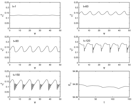
Figure 1: Time evolution of the state parameter $\nu_{*}^{2}$ along the string worldsheet for an elliptic configuration of a loop with a bosonic current in the magnetic regime, having large ellipticity $e=0.6$ and velocity parameter $\epsilon=1$, and with a phase parameter $\ell=3$ (and $A=3$, $B=-0.2$). In the last panel the variation of the energy shows two important things. On the one hand the small peaks in the graph are an evidence that the loop size decreases because the initial velocity has been reduced. On the other hand, nearly at the end of the simulation, the rare variation of the energy gives a signal of the shocks produced along the loop string. The relative variation of the total energy, shown on the last panel, is still rather small even as the simulation reaches its very end. The situation is similar for the angular momentum, and the simulation eventually breaks down.

Another important effect that may take place along a superconducting loop is the appearance of kinks. These are regions where the curvature of the string becomes discontinuous. We found that giving an extra dimension for the loop to evolve into did not suppress the appearance of kinks. Fig. 2 shows the evolution of a loop in the electric regime, and therefore using the equation of state given by Eq. (36). In this case again, the simulation shows that $2\ell$ kinks are being formed at points along the loop. To illustrate this point further, we plotted in Fig. 3 the curvature of the loop as a function of the spacelike string internal coordinate $\psi$. This is, in general, given by formal

$$K^{\mu}=\eta^{\rho\nu}K_{\rho\nu}^{\mu},$$ (50)

i.e., in the case at hand,

$$K^{2}=(w_{\bot 1}^{\rho}K_{\rho})^{2}+(w_{\bot 2}^{\rho}K_{\rho})^{2},$$ (51)

where

$$w_{\bot 1}^{\rho}K_{\rho} = \frac{1}{\Delta_{3}n^{2}\dot{\zeta}^{2}}\left[\left(n^{2}-\beta^{2}\right)\left(\ddot{y}z^{\prime}-\ddot{z}y^{\prime}\right)+2\beta\dot{\zeta}^{2}\left(y^{\prime}\dot{z^{\prime}}-z^{\prime}\dot{y^{\prime}}\right)+\dot{\zeta}^{4}\left(y^{\prime}z^{\prime\prime}-z^{\prime}y^{\prime\prime}\right)\right],$$ (52)

$$w_{\bot 2}^{\rho}K_{\rho} = \frac{1}{\Delta_{3}n^{2}\dot{\zeta}^{2}}\left[(n^{2}-\beta^{2})(\Delta_{3}\ddot{x}-\Delta_{2}\ddot{y}+\Delta_{1}\ddot{z})-2\beta\dot{\zeta}^{2}(\Delta_{3}\dot{z^{\prime}}-\Delta_{2}\dot{y^{\prime}}+\Delta_{1}\dot{z^{\prime}})-\dot{\zeta}^{4}(\Delta_{3}x^{\prime\prime}-\Delta_{2}y^{\prime\prime}+\Delta_{1}z^{\prime\prime})\right]\!\!.$$ (53)

It is clear in the figure that where kinks appear, large variations of the curvature are developed, showing that the kinks are not gauge artifacts but really occur. As expected, the location of the kinks corresponds to the points with large curvature. In general the effects found in the two dimensional planar case are still present in three dimensions. They are however usually affected (or even initiated) by the transverse perturbation in $z$.

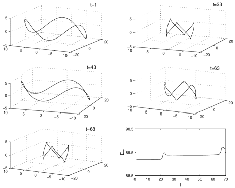
Figure 2: Configuration evolution in the electric case with bosonic currents with the same ellipticity as in Fig. 1, $\epsilon=0.1$ and $A=3$ ($B=0$). One clearly sees the development of six kinks corresponding to twice the phase parameter $\ell=3$. In this case, the peaks seen in the energy are formed at the same time as the kinks are present.

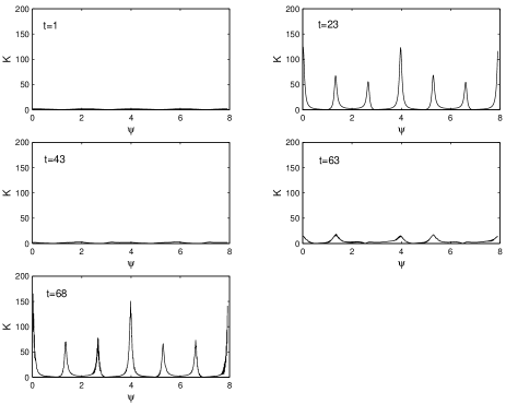
Figure 3: Invariant magnitude $K=\sqrt{K^{2}}$ of the curvature, from Eq. (51), for the configuration shown in Fig. 2.

In some cases, the string loop shows points where intercommutation, which is not taken into account in our code, should be occurring. A systematic analysis shows that a loop in three dimensions tends to fold on itself in any regime, magnetic or electric. This is similar to what happens to Goto-Nambu loops for which it was even argued that this intercommuting process could be the leading process for a string network to loose energy reliable ; topoconj . The conclusions that can be drawn from this fact for a superconducting string network are therefore the same, and will be discussed later. In Fig. 4 is shown an example of such a missed intercommutation for a loop in the electric case.

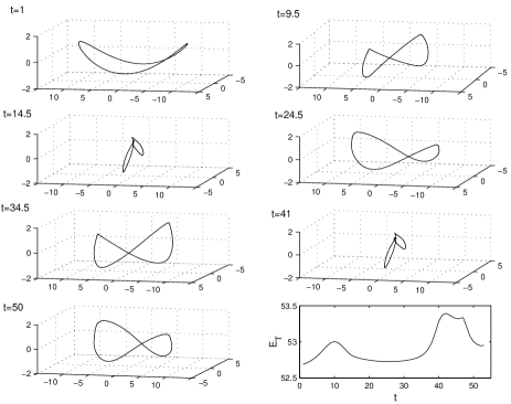
Figure 4: A typical string loop configuration showing points where intercommutation should take place, with $\ell=2$, ellipticity $e=0.3$, $A=1$, $B=0.1$, and $\nu_{*0}^{2}=0.1$. At these points, two loops should be formed and the subsequent evolution given by the code is no longer physically relevant.

Another possibility that is open for a loop to leave the region where the elastic description is valid is to locally have one of its squared perturbation velocity, $c_{{}_{\rm L}}^{2}$ in the magnetic regime, or $c_{{}_{\rm T}}^{2}$ in the electric regime, becoming negative. In the latter case, the tension reaches negative values and the string actually behaves like a spring. In Fig. 5 is shown the evolution of the longitudinal perturbation velocity as a function of the spacelike parameter along the string loop at different instants of time in a typical example for which the dynamical evolution of the loop drives it out of the elastic regime when $c_{{}_{\rm L}}^{2}$ becomes less than zero. Whatever happens past this time is presumably not accounted for correctly by the program which, being an effective macroscopic description, does not recognize the instability at the microscopic level.

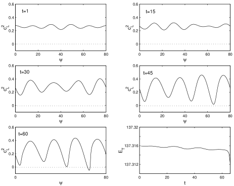
Figure 5: Time evolution of the squared perturbation velocity, $c_{{}_{\rm L}}^{2}$, in the magnetic regime for a bosonic superconducting loop. The dynamics drives the loop out of the elastic regime, as seen on the last evolution panel, in which one finds a region having $c_{{}_{\rm L}}^{2}\leq 0$. The last panel shows the total energy integrated along the loop as a function of time: its constancy up to the point where $c_{{}_{\rm L}}^{2}$ becomes negative reveals that nothing particular took place and the physical description can be trusted. Past this point, the energy is very badly conserved and the program, as expected, has difficulties handling the problem. This figure is for $A=2$ and $B=0$.

All these results are reminiscent of what had previously been obtained in the two dimensional case 2D . There now is no more ambiguity about them being projection artifacts. The conclusions derived in the 2D case therefore still apply.

IV.2 Fermionic Current

In this section, we consider current–carrying cosmic strings with fermionic currents, obeying the equation of state (40). The behavior in this case follows somewhat that observed in the bosonic case: the loop can fold on itself and leave the elastic domain. We shall exemplify both cases in turn, but first let us remark the important following point. Since in the fermionic case the equation of state is self-dual, there cannot be any qualitative difference between the magnetic and the electric regimes at the level of the equations of motion. However, the two perturbation velocities are not equal and the string may become unstable only with respect to transversal perturbations. As a result, the dynamical evolution of the string can lead it to develop only kinks, although in this case we cannot say that the effect is exclusive of the electric or magnetic regime. In Figs. 6 and 7, we show the time evolution and the curvature (snapshots at different times) for a loop with fermionic current, again with phase parameter $\ell=3$ and initial value of the state parameter set as $\nu_{*0}^{2}=0.1$. The appearance of kinks is seen as the curvature of the string becomes discontinuous. When the kink is formed the total energy is no longer conserved and the simulation ends.

Similarly to the case of cosmic string loops endowed with bosonic currents, loops with fermionic currents can fold on themselves, exhibiting points where intercommutation should take place, and with very much the same rate of occurrence in the evolution. Self-intercommutation for loops loosing their energy again seems to be in this case a favored mode.

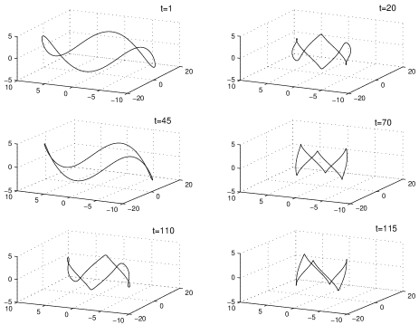
Figure 6: Configuration evolution for fermionic equation of state. In this case, the shape of the loop changes until kinks are formed along the string, at which point the elastic string description ceases to be sufficient. Quasi kinks are formed first, that are subsequently rounded off, until the actual kinks really form. Here, and in the following figure, the parameters $A=3$ and $B=0.2$ have been used.

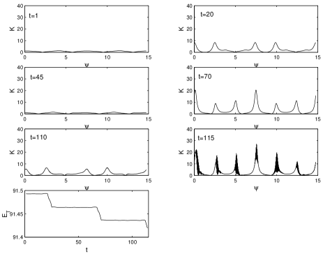
Figure 7: Time evolution of curvature against the point labeling function $\psi$ for the configuration of the Fig. 6. The curvature in this example varies almost by two orders of magnitude. As in the bosonic case, the variations of the energy give a signal of the kinks formation.

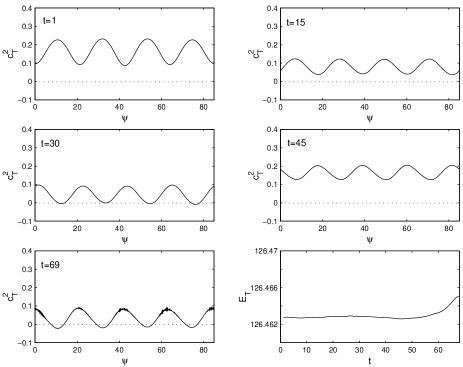
Figure 8: Time evolution of the speed of transversal perturbations for a cosmic string loop with fermionic currents (with $A=2$ and $B=-0.2$). The dynamical evolution of the loop drives it out or the elastic regime, where $c_{{}_{\rm T}}^{2}\leq 0$.

The string loop can also leave the domain of validity of the elastic formalism when $c_{{}_{\rm T}}^{2}$ becomes negative. Fig. 8 depicts the time evolution of the transverse velocity $c_{{}_{\rm T}}^{2}$ up to the point where it vanishes. The velocity here is shown as a function of the spacelike string parameter $\psi$. The same remarks as for bosonic strings apply, in particular concerning the non conservation of the total energy whenever the elastic regime is left. Note here the appearance of a numerical instability that propagates along the string and that is seen in the form of (unphysical) oscillations.

V Discussions and Conclusions

This work is the direct follow-up of previously discussed two dimensional string loop simulations 2D . It extends this old work in two directions. First it now provides results about the dynamics of such string loops in three dimensions, thereby answering the question as to whether the observed effects were actually physical or mere projection artifacts. This new simulation clearly shows that indeed the effects presented in Ref. 2D are physical. Another extension of Ref. 2D that is done here concerns the equation of state, which can now describe fermionic fermions0 currents as well.

In the case of strings endowed with spacelike bosonic currents, it was shown that most of the loops develop shock. These shocks are seen as discontinuities in the current and occur because the squared longitudinal perturbation velocity $c_{{}_{\rm L}}^{2}$ can become negative. In the electric regime of timelike currents, it is the squared transverse perturbation velocity $c_{{}_{\rm T}}^{2}$ that can vanish and reverse its sign. As it turns out, this implies that kinks, namely regions of discontinuous curvature, develop.

Fermionic strings, being described by an equation of state for which only the squared transverse perturbation velocity can become negative, are subject only to the possibility of building kinks, and this in a way that is independent of the spacelike or timelike nature of the underlying current since the relevant equation of state is self-dual.

In both cases, fermionic and bosonic currents, and for whatever kind of current, the loops tend to fold on themselves, generating contact points where intercommutation should occur. The almost systematic occurrence of such configuration leads us to conclude that one may divide superconducting string loops into essentially two species: those loops which tend to divide into smaller loops, and the other ones that are identified with the proto-vortons of other authors vortons2 . Our results tend to indicate that the latter category is much less populated than the former, as was already postulated in earlier investigations vortons2 . It also implies that these intercommutations will be, in the case of superconducting cosmic strings, much more frequent than in the case of ordinary strings.

Now when a string loop self-intercommutes, the topological stability that confines the Higgs and other particles inside the defect is raised and some of these particles are expelled away. Although stable while contained in the defects, these particles are often unstable. In particular, strings are expected to form at the Grand Unified (GUT) scale, and the relevant Higgs and gauge fields to decay therefore almost instantaneously by cosmological standards. These particles will then initiate showers of lower mass ones dividing the original energy. This is the mechanism that is at work in most Top-Down scenarios topdown of Ultra High Energy Cosmic Rays (UHECR) whose origin is still mysterious uhecr . Ordinary cosmic strings do not produce much of these particles, because intercommutations are not that frequent in Goto-Nambu strings since most of the energy of the network in that case is expected to be lost through gravitational radiation book . In fact gillkibble , the resulting flux is found a disappointing ten orders of magnitude below the observed one. In the case of current-carrying strings, loops have a higher probability of self-intercommuting, so the mechanism is enhanced accordingly.

The proto-vorton case now takes us to the rare configurations that do not intercommute frequently. Note at this point that the scarcity of these states is not enough to ensure the vorton excess problem to be altogether alleviated. Indeed, for GUT scale vortons, the ratio between proto-vortons and doomed loops should already be much less than $10^{-20}$ in order for the present-day vortons not to dominate the Universe vortons2 if the resulting vortons are stable over cosmologically relevant timescales.

Gathering all the results obtained over the recent years, we now find the following: for a realistic underlying microscopic model, the equation of state is such that at least one of the perturbation propagation speed can become imaginary, leading to possible instabilities. The main result of the present paper is to show that these instabilities will systematically develop in every loop as it evolves. As a result, the elastic treatment turns out to be valid for limited periods of time and one must resort to the full microscopic description in between.

The elastic description breaks down in two possible ways, namely through the formation of kinks or shocks. In both cases, the meaning is that the microstructure should be taken into account. In particular, close to these points, it is no longer appropriate to consider the string as effectively two dimensional and we must consider the effects that are due to the finite thickness.

First of all, kinks cannot exist if the string is a tube instead of a Dirac line as it would be impossible for instance to match the Higgs field and its derivatives, as is however required by the underlying field theory, at the points where the curvature is discontinuous. Therefore, the string must somehow find a way of smoothing, which means in that context loosing energy. The only non kinematical (in the sense of necessarily breaking the elastic description) way of realizing that is through particle emission, and we are led to conclude that, as in the case of intercommutation, but for completely different reasons, some particles (current carriers, but also Higgs and gauge fields) will be radiated away as the kinks develop. Note also that the current-carrier is indeed likely to get out of the string since, as the string curvature increases, the carrier momentum acquires an orthogonal-to-the-worldsheet component thanks to which the wavefunction is spread over larger distances, thereby effectively increasing the probability for the particle to tunnel out. This mechanism can ease the vorton excess problem while in the same time providing more efficiency for UHECR production through Top-Down scenarios.

Shocks develop only for bosonic spacelike currents. In this case, the state parameter $\nu$, which would end up being discontinuous were the shock actually occurring, is well represented by the collective momentum of the trapped particles neutral ; enon0 , this momentum being always less than the rest mass of the carrier particles themselves in order for the confinement to take place. As we argued before 2D , it is rather dubious that actual shock could form in cosmic strings, as the shocks are always accompanied, either followed or preceded, by a transient region in which $c_{{}_{\rm L}}^{2}\leq 0$. However, in this region, the momentum of the carrier is higher or at least of the same order as its rest mass. Therefore, it is energetically favored to some of the trapped particles to move out of the string.

In all the situations which we have studied, we found that the expected dominant effect was particle radiation. We are therefore led to the conclusion that an elastic treatment of cosmic strings is not completely appropriate. It should be supplemented with some semi-classical, non conservative, forces. The dissipative effect then introduced can serve to ease the vorton excess problem, while providing new interesting ways to produce UHECR.

- (1) T. W. B. Kibble, J. Phys. A 9, 1387 (1976); Phys. Rep. 67, 183 (1980).
- (2) E. Witten, Nucl. Phys. B249, 557 (1985).
- (3) E. P. S. Shellard and A. Vilenkin, “Cosmic strings and other topological defects”, (Cambridge University Press, Cambridge, UK, 1994); See M.B. Hindmarsh and T.W.B. Kibble, Rep. Prog. Phys. 58, 477 (1995) for a recent review on topological defects in general.
- (4) T. Goto, Prog. Theor. Phys. 46, 1560 (1971); Y. Nambu, in “Symmetries and Quark model”, Ed. R. Chand, 269, Gordon and Breach (1970); Phys. Rev. D10, 4262 (1974).
- (5) A. Babul, T. Piran and D. N. Spergel, Phys. Lett. B 202, 307 (1998).
- (6) P. Peter, Phys. Rev. D45, 1091 (1992); Phys. Rev. D46, 3335 (1992).
- (7) P. Peter, Phys. Rev. D46, 3335 (1992); Phys. Rev. D47, 3169 (1993).
- (8) B. Carter, Covariant mechanics of simple and conducting strings and membranes, it in “The Formation and Evolution of Cosmic Strings”, G. Gibbons, S. Hawking and T. Vachaspati Eds., 143 (Cambridge University Press, Cambridge, UK, 1990); B. Carter, Phys. Lett. B 238, 166(1990); B. Carter, Phys. Lett. B 224, 61 (1989); B. Carter, Nucl. Phys. B 412, 345 (1994).
- (9) B. Carter and P. Peter, Phys. Rev. D52 R1744 (1995).
- (10) A. Vilenkin, Phys. Rev. D41, 3038 (1990); X. Martin, Phys. Rev. Lett. 74, 3102 (1995).
- (11) N. K. Nielsen and P. Olesen, Nucl. Phys. B 291,829 (1987).
- (12) P. Peter and C. Ringeval, Fermionic current-carrying cosmic strings: zero-temperature limit and equation of state, hep-ph/0011308, to appear in the proceedings of the Journées Relativistes, Dublin (2001).
- (13) X. Martin and P. Peter, Phys. Rev. D61, 043510 (2000).
- (14) A.L. Larsen, Class. Quantum. Grav. 10, 1541 (1993); A. L. Larsen and M. Axenides, Class. Quantum Grav. 14, 443 (1997); B. Carter, P. Peter and A. Gangui, Phys. Rev. D55, 4647 (1997); A. Gangui, P. Peter and C. Boehm, Phys. Rev. D57, 2580 (1998).
- (15) G. V. Vlasov, Discontinuities on strings, hep-th/9905040.
- (16) C. Ringeval, Phys. Rev. D63, 063508 (2001).
- (17) D. P. Bennett and F. R. Bouchet, Phys. Rev. D41, 2408 (1990); D. P. Bennett and F. R. Bouchet, Phys. Rev. Lett. 63, 2776 (1989); F. R. Bouchet, D. P. Bennett and A. Stebbins, Nature (London)335 (1988); B. Allen, R.R. Caldwell, S. Dodelson, L. Knox, E.P.S. Shellard and A. Stebbins, Phys. Rev. Lett. 79, 2624 (1997).
- (18) R. L. Davis and E. P. S. Shellard, Phys. Rev. D38, 4722 (1988); Nucl. Phys. B 323, 209 (1989); B. Carter, Ann. N.Y. Acad. Sci., 647, 758 (1991); B. Carter, Phys. Lett. 238, 166 (1990); Proceedings of the XXXth Rencontres de Moriond, Villard–sur–Ollon, Switzerland, 1995, Edited by B. Guiderdoni and J. Tran Thanh Vân (Editions Frontières, Gif–sur–Yvette, 1995).
- (19) R. Brandenberger, B. Carter, A. C. Davis and M. Trodden, Phys. Rev. D54, 6059 (1996); B. Carter and A. C. Davis, Phys. Rev. D61, 123501 (2000).
- (20) J. Linsley, Phys. Rev. Lett. 10 146 (1963); Proc. 8th International Cosmic Ray Conference 4, 295 (1963); R. G. Brownlee et al., Can. J. Phys. 46 S259 (1968); M. M. Winn et al., J. Phys. G 12 653 (1986); M. A. Lawrence, R. J. O. Reid and A. A. Watson, J. Phys. G Nucl. Part. Phys. 17, 733 (1991); D. J. Bird et al., Phys. Rev. Lett. 71, 3401 (1993); Ap. J. 424, 491 (1994); ibid. 441, 144 (1995); N. Hayashida et al., Phys. Rev. Lett. 73, 3491 (1994); S. Yoshida et al., Astropart. Phys. 3, 105 (1995); M. Takeda et al., Phys. Rev. Lett. 81, 1163 (1998).
- (21) T. W. Kephart and T. J. Weiler, Astropart. Phys. 4, 271 (1996); S. Bonazzola and P. Peter, Astropart. Phys. 7, 161 (1997); E. Huguet and P. Peter, Astropart. Phys. 12, 277 (2000).
- (22) A. J. Gill and T. W. B. Kibble, Phys. Rev. D50 3660 (1994).
- (23) A. Riazuelo, N. Deruelle and P. Peter, Phys. Rev. D61, 123504 (2000).
- (24) B. Carter, Phys. Rev. D41, 3869 (1990).
- (25) J.-P. Uzan and P. Peter, Phys. Lett. B 406, 20 (1997).
- (26) B. Carter and X. Martin, Ann. Phys. (N.Y.) 227, 151 (1993); X. Martin, Phys. Rev. D50, 7479 (1994).
- (27) See G. Sigl, hep-ph/0109202 (2001); Science 291, 73 (2001); P. Bhattacharjee and G. Sigl, Phys. Rep. 327, 109 (2000) and references therein.