Lattice QCD and the Unitarity Triangle

Abstract

Theoretical and computational advances in lattice calculations are reviewed, with focus on examples relevant to the unitarity triangle of the CKM matrix. Recent progress in semi-leptonic form factors for $B\to\pi l\nu$ and $B\to D^{*}l\nu$, as well as the parameter $\xi$ in $B^{0}$-$\bar{B}^{0}$ mixing, are highlighted.

1 Introduction

To test the CKM picture of $CP$ and flavor violation, a combination of theory and experiment is needed. A vivid way to summarize the need for redundant information is the unitarity triangle (UT), sketched in Fig. 1.

Figure 1: Unitarity triangles: on the left is the “tree” triangle; on the right, the “mixing” triangle.

It depicts two triangles, $B\gamma A$, which can (in principle) be determined from tree processes (e.g., semi-leptonic decays), and $\alpha C\beta$, in which the amplitude for $B^{0}$-$\bar{B}^{0}$ mixing is involved Kronfeld (2001). The “tree” triangle can, for the sake of argument, be taken as a measurement of the CKM matrix. Then, the “mixing” triangle tests whether new physics must be invoked to explain $B^{0}$-$\bar{B}^{0}$ mixing.

To obtain the sides $A$, $B$, and $C$ of these triangles one must calculate hadronic properties from first principles of QCD. Here “calculate” implies that a reliable error estimate is given: one that includes all sources of uncertainty. Lattice gauge theory is well suited to the task: semi-leptonic form factors and the mixing matrix elements are conceptually straightforward. Indeed, according to Martin Beneke Beneke (2001), “[the] standard UT fit is now entirely in the hands of lattice QCD (up to, perhaps, $|V_{ub}|$).”

Until recently, lattice QCD has been burdened by something called the quenched approximation (explained below). A bit of good news is that the available computer power is now sufficient to get rid of this approximation Ali Khan (2000, 2000); Bernard (2001). Another bit of good news is that several lattice groups have used the quenched approximation in the spirit of a blind analysis: although quenching could change the central value, one can analyze all other uncertainties as if the underlying numerical data were real QCD. This exercise has left us with several quantities, including those needed in the UT fits, with full error analyses, apart from quenching. In the next few years, we should have full QCD calculations with a complete assessment of the uncertainties, and thereafter the uncertainties can be incrementally reduced.

Because it is important to understand the theoretical uncertainties, this talk will start by sketching where they arise. Most reviews focus too much on central values, so, even when turning to numerical results, the focus here is on the error bars.

The paper ends with a short swim through the “Octopus’s Garden”, that is, some recent work by Nathan Isgur, who passed a way a few weeks before Heavy Flavors 9 convened. The symposium, and this paper, are dedicated to his memory.

2 Uncertainties in Lattice Calculations

Lattice QCD calculates matrix elements by integrating the functional integral, using a Monte Carlo with importance sampling. The Monte Carlo leads to (correlated) statistical error bars. This part of the method is well understood for quenched QCD and, these days, rarely leads to controversy. When conflicting results arise, they originate in different treatments of the systematics. The consumer probably does not need to know how the Monte Carlo works, but should develop an intuition of how the systematics work.

The main tool for controlling systematics is effective field theory. In this talk, we are concerned mostly with three classes of effects: those connected with the lattice spacing $a$, the heavy quark mass(es) $m_{Q}$, and the light quark mass(es) $m_{q}$. Inside the computer there is a hierarchy of scales

$$m_{q}\ll\Lambda\ll m_{Q},\;\pi/a,$$ (1)

although in practice $\pi/a$ is a only several GeV, and the “light” quarks are never as light as the up and down quarks. The QCD scale $\Lambda$ gauges the size of power corrections; experience suggests it is 700 MeV, give or take a factor of $\sqrt{2}$. With familiar techniques of effective field theory, lattice theorists can control the extrapolation of artificial, numerical data to the real world, provided the data start “near” enough. Similarly, non-experts usually have an intuition of how effective field theories work, so they can check, on the back of the envelope, whether systematic errors have been treated sensibly.

The notable exception to the rule of effective field theory is the valence, or quenched, approximation. Consider the pictures in Fig. 2.

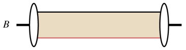
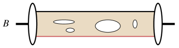
Figure 2: Quenched approximation: processes on the left are incorporated “exactly”, whereas processes on the right are not computed, but modeled with a shift in the bare couplings.

The one on the left depicts a meson made of a valence quark and anti-quark, bound by a shmear of gluons. The gluons can also create virtual quark-antiquark pairs, leading to the picture on the right. These are computationally very costly. The quenched approximation omits them but compensates the omission with a shift in the bare couplings. This is analogous to a dielectric, where $g_{0}^{2}\to g_{0}^{2}\epsilon$. Quenching retains many effects, such as retarded gauge potentials, that are omitted in, say, the quark model. It is also the first term in a systematic expansion Sexton and Weingarten (1997).

The quenched approximation can fall short of reproducing chiral logarithms of the form $\ln(\Lambda^{2}/m_{q}^{2})$ Morel (1987); Sharpe (1990); Bernard and Golterman (1992, 1994). Figure 3 shows some quark-line configurations that generate, at the hadronic level, meson loops.

Figure 3: Quark line configurations that lead to meson loops. Adapted from Ref. Bardeen et al. (2001).

The quenched approximation includes (b), but not (a) or (c). As a consequence, some pion loops are omitted, and $\eta^{\prime}$ loops are mistreated. A better situation is a “partially quenched” theory, with dynamical quark loops, but, possibly, $m_{\mathrm{valence}}\neq m_{\mathrm{sea}}$. Then features like the $\eta^{\prime}$-$\pi$ splitting emerge, and it is possible to relate the partially quenched theory to full QCD using chiral perturbation theory. We shall return to chiral logs in the next section, when discussing $B^{0}$-$\bar{B}^{0}$ mixing.

To understand lattice spacing effects Symanzik suggested matching lattice gauge theory to continuum QCD Symanzik (1983a):

$${\cal L}_{\rm lat}\doteq{\cal L}_{\rm QCD}+\sum_{i}a^{s_{i}}K_{i}(g^{2},m_{q}a;\mu){\cal O}_{i}(\mu).$$ (2)

The right-hand side is a local effective Lagrangian (LE${\cal L}$) renormalized in some continuum scheme; details of the scheme are not important. Discretization effects are, of course, short-distance effects, so as usual in an effective field theory, they are lumped into the coefficients $K_{i}$.

There are two key points to the Symanzik effective field theory. First, if $\Lambda a$ is small enough, the $\sum_{i}$ can be treated as a perturbation. For example, for the proton mass

$$m_{p}(a)=m_{p}-aK_{\sigma F}(c_{\rm SW})\langle p|\bar{\psi}\sigma\cdot F\psi|p\rangle$$ (3)

using the leading term for Wilson fermions as an example. Here $c_{\rm SW}$ is the so-called clover coupling, and $K_{\sigma F}=(1-c_{\rm SW})/4+O(\alpha_{s})$. Second, to reduce lattice spacing effects, one can tune $c_{\rm SW}$ so that $K_{\sigma F}$ vanishes or, in practice, is $O(\alpha_{s}^{\ell})$ or $O(a)$. Thus, the Symanzik effective field theory shows that lattice artifacts can be reduced through short-distance process-independent methods. Indeed, for light hadrons a combination of this Symanzik improvement and extrapolation in $a^{2}$ gives continuum QCD results with very well understood uncertainties (modulo quenching).

With the bottom and charmed quarks, the mass is large in lattice units: $m_{b}a\sim$1–2 and $m_{ch}a$ about a third of that. The split in the LE${\cal L}$ between QCD and small correction breaks down, because there are terms in the $\sum_{i}$ in Eq. (3) that go like $(m_{Q}a)^{n}$. It will not be possible to reduce $a$ enough to make $m_{b}a\ll 1$ for a long time: Moore’s Law suggests 15–25 years. There are, nevertheless, several ways to treat heavy-light hadrons in lattice calculations, all of which appeal to HQET in some way. Table 1 lists the most widely used methods.

#	method	Ref.	how HQET enters
1.	static approximation	Eichten (1988); Eichten and Hill (1990)	${\cal L}_{\rm static}=-\bar{h}D_{4}h$
2.	lattice NRQCD	Lepage and Thacker (1988); Thacker and Lepage (1991)	discretization of first few terms of HQET
3.	extrapolation from below charm	ad hoc	results with small $m_{Q}$ fit to Taylor series in $1/m_{Q}$
$3^{\prime}\!.$	$3+1$	ad hoc	as in method 3
4.	“Fermilab”	El-Khadra et al. (1997); Kronfeld (2000)	match lattice to QCD, term-by-term in HQET

Table 1: Widely used methods for heavy quarks in lattice gauge theory.

In lattice NRQCD and in the Fermilab method, it is possible to set $m_{Q}=m_{b}$, even when $a^{-1}\sim m_{b}$. There are, of course, uncertainties involved, but a grasp of the basics of heavy-quark theory is enough understand them.

A convenient way to contrast the uncertainties in the various methods is to match lattice gauge theory to (continuum) HQET Kronfeld (2000). Instead of Eq. (3) one writes

$${\cal L}_{\rm lat}\doteq{\cal L}_{\rm HQET}=\sum_{n}{\cal C}_{n}^{\mathrm{lat}}{\cal O}_{n}=-m_{1}\bar{h}h-\bar{h}D_{4}h+\frac{\bar{h}\kern 1.0ptD\kern-8.0ptD\kern 1.0pt^{2}h}{2m_{2}}+\frac{\bar{h}i\kern 1.0pt\Sigma\kern-8.0pt\Sigma\kern 1.0pt\cdot\kern 1.0ptB\kern-8.0ptB\kern 1.0pth}{2m_{\cal B}}+\cdots.$$ (4)

The operators ${\cal O}_{n}$ on the right hand side are the same as in the HQET description of continuum QCD. The short-distance coefficients ${\cal C}_{n}^{\mathrm{lat}}$, on the other hand, are not the same, because there are two short distances, $a$ and $1/m_{Q}$. Heavy-quark lattice artifacts are, thus, isolated into the mismatch ${\cal C}_{n}^{\mathrm{lat}}-{\cal C}_{n}^{\mathrm{cont}}$. In lattice NRQCD and in the Fermilab method, these mismatches can be reduced, along the same lines as reducing $K_{\sigma F}$ in the Symanzik program. In recent work, they are controlled to several percent or less.

Most work with method 3 has chosen normalization conditions for which the mismatch in the kinetic and chromomagnetic terms, although formally $O(m_{Q}a)^{2}$, is quite large in practice. It is also not well understood how this mismatch is amplified when extrapolating linearly or quadratically in $1/m_{Q}$ from $m_{Q}\sim 1$ GeV up to $m_{b}$.

3 Lattice Calculations

We now turn our attention to some of the most interesting recent lattice calculations in $B$ physics. The discussion focuses on the error bars, and central values are deferred to the next section. We consider the ratio $\xi$ for $B$-$\bar{B}$ mixing in unquenched QCD, and the semi-leptonic decays $B\to\pi l\nu$ and $B\to D^{*}l\nu$ for $|V_{ub}|$ and $|V_{cb}|$ in quenched QCD.

3.1 Neutral Meson Mixing

The mass difference of neutral $B$ meson $CP$ eigenstates is

$$\Delta m_{B^{0}_{q}}=\frac{G_{F}^{2}m_{W}^{2}S_{0}}{16\pi^{2}}|V_{tq}^{*}V_{tb}|^{2}\eta_{B}\langle\bar{B}_{q}^{0}|Q_{q}^{\Delta B=2}|B_{q}^{0}\rangle+\textrm{new physics?}$$ (5)

where $q\in\{d,\,s\}$, $S_{0}$ is an Inami-Lim function, $\eta_{B}$ is a short-distance QCD correction, and $Q_{q}^{\Delta B=2}$ is a four-quark operator in the $\Delta B=2$ electroweak Hamiltonian. Note that new physics could compete with the Standard Model. The matrix element of $Q_{q}^{\Delta B=2}$ is usually written

$$\langle\bar{B}_{q}^{0}|Q_{q}^{\Delta B=2}|B_{q}^{0}\rangle=\frac{8}{3}m^{2}_{B_{q}}f^{2}_{B_{q}}B_{B_{q}},$$ (6)

but lattice QCD gives $\langle\bar{B}_{q}^{0}|Q_{q}^{\Delta B=2}|B_{q}^{0}\rangle$ and $f_{B_{q}}$ (from $\langle 0|A^{\mu}_{bd}|B_{q}^{0}\rangle$) individually. This traditional separation turns out to be useful when looking at chiral logs.

Conventional wisdom says that the uncertainties in $B_{B_{q}}$ and in $\xi^{2}=f_{B_{s}}^{2}B_{B_{s}}/f_{B_{d}}^{2}B_{B_{d}}$ are “easy” to control, because they are ratios. At Lattice ’01, Norikazu Yamada of JLQCD reported on new results Yamada et al. (2001) that suggest otherwise. The JLQCD collaboration is mounting a large project to carry out calculation with the loops of $n_{f}=2$ flavors of quarks. Figure 4 compares their previous quenched work for $f_{B_{q}}$ with their new (and still preliminary) work with $n_{f}=2$.

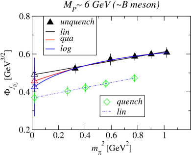
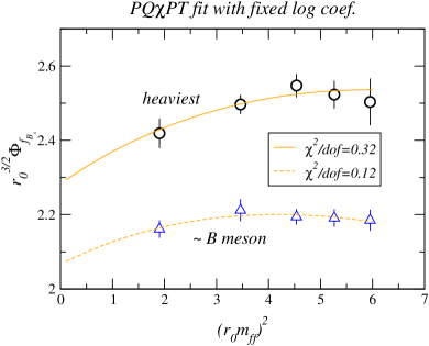
Figure 4: Recent calculations of the decay constant $\Phi_{B}=f_{B}\sqrt{m_{B}}$ from JLQCD.

In the spirit of a blind analysis, the definition of $\Phi_{f_{Bq}}$ is not so important. The important matter is whether the curve is a straight line, or whether there is any curvature as a function of the light quark mass. (Because the pseudoscalar $m_{\pi}^{2}\propto m_{q}$, the horizontal axis is, essentially, the light quark mass.)

The quenched approximation (diamonds in Fig. 4) shows no evidence of curvature. With $n_{f}=2$ (triangles in Fig. 4), however, allowing for curvature obtains a better fit. In fact, curvature is expected from chiral logarithms. Meson loops with fixed spectator mass $m_{s}$ and varying sea quark mass $m_{f}$ contribute to $f_{B_{s}}$ Sharpe and Zhang (1996)

$$\Delta f_{B_{s}}=c_{0}+c_{1}m^{2}_{\eta_{ff}}-\frac{1+3g^{2}}{(4\pi f_{\pi})^{2}}m^{2}_{\eta_{sf}}\ln\left(\frac{m^{2}_{\eta_{sf}}}{m^{2}_{\eta_{ss}}}\right),$$ (7)

where $\eta_{qq^{\prime}}$ denotes a pseudoscalar meson with constituents $q$ and $q^{\prime}$. From the $D^{*}$ width, $3g^{2}\approx 1.04$ Anastassov et al. (2001). The second plot in Fig. 4 shows that Eq. (7) describes the points well.

It is worth making a few remarks about this kind of analysis. The formula for $f_{B_{d}}$ (where the spectator and sea quarks have the same mass) is slightly different, so it is difficult to display all chiral log effects on one plot. Nevertheless, one can see from Fig. 4 that the effect is to increase $f_{B_{s}}/f_{B_{d}}$. The chiral logs for $B_{B_{q}}$ are multiplied by $1-3g^{2}\approx 0.04$, so the $B_{B_{s}}/B_{B_{d}}$ is almost insensitive to them. Therefore, the chiral logs in the ratio $\xi$ come almost completely from $f_{B_{s}}/f_{B_{d}}$. One concludes that $\xi$ may have been underestimated in the quenched approximation. A new estimate, based on JLQCD and previous work, is given below.

3.2 $B\to\pi l\nu$ and $V_{ub}$

The semi-leptonic decay $B\to\pi l\nu$ is mediated by a $b\to u$ transition. The decay rate is

$$\frac{d\Gamma}{dE}=\frac{G_{F}^{2}m_{B}p^{3}}{12\pi^{3}}|V_{ub}|^{2}|f_{+}(E)|^{2},$$ (8)

where $v=p_{B}/m_{B}$ is the $B$ meson’s velocity, $E=v\cdot p_{\pi}$, and $p^{2}=E^{2}-m_{\pi}^{2}$. The form factor $f_{+}(E)$ is a linear combination of the form factors $f_{\perp}(E)$ and $f_{\parallel}(E)$, defined through the matrix element of the vector current

$$\langle\pi|V^{\mu}|B\rangle=\sqrt{2m_{B}}\left[v^{\mu}f_{\parallel}(E)+p^{\mu}_{\perp}f_{\perp}(E)\right].$$ (9)

The pion energy $E$ is related to $q^{2}=m_{B}^{2}+m_{\pi}^{2}-2m_{B}E$. Chiral symmetry and heavy-quark symmetry are simpler to follow with $f_{\parallel}$ and $f_{\perp}$ considered as functions of $E$, rather than $f_{+}$ considered as a function of $q^{2}$. For example, heavy-quark symmetry suggests relations between $B$ and $D$ decays with the same $E$. In principle, one would like to compare the $E$ dependence of experimental measurements with lattice calculations. Discretization uncertainties are smallest for low $E$, where phase space suppresses the event rate. Therefore, lattice calculations and experimental measurements will have to be combined in the way that minimizes the error on $|V_{ub}|$.

In the past year or so, four new quenched calculations of $f_{+}(E)$ for $B\to\pi l\nu$ appeared, using several different methods Bowler et al. (2000); Abada et al. (2000); El-Khadra et al. (2001); Aoki et al. (2001). It is, thus, timely to compare and contrast. In addition to discretization effects at large $pa$, there is evidence for considerable dependence on the light spectator quark mass El-Khadra et al. (2001).

The calculations of UKQCD Bowler et al. (2000) and APE Abada et al. (2000) use method 3, so they have discretization errors of order $(m_{Q}a)^{2}$. They keep $m_{Q}<1.2m_{c}$ and extrapolate up to $m_{b}$ linearly or quadratically in $1/m_{Q}$. The quark masses used in Ref. Bowler et al. (2000) are shown in Table 2. Those in Ref. Abada et al. (2000) are a bit larger, which is better for HQET but worse for the discretization errors. In these papers models are used to extrapolate to the full kinematic range of $E$. It is better to think of these calculations as computing the model parameters in $D$ decays, and then invoking HQET to make predictions for TABLE 2. Heavy quark masses used in Ref. Bowler et al. (2000). Note that $m_{\textrm{pole}}<m^{\rm RI}$. $\kappa$ $am_{Q}$ ${m}^{\rm RI}_{Q}$ $M_{P}$ (GeV) (GeV) 0.1200 0.485 1.52 $2.035(5)$ 0.1233 0.374 1.23 $1.771(5)$ 0.1266 0.268 1.02 $1.483(5)$ 0.1299 0.168 0.69 $1.157(5)$
$B$ decays. The error associated with the assumptions are, at least to me, not transparent.

The calculation of El-Khadra et al. El-Khadra et al. (2001) uses the Fermilab method, and the calculation of JLQCD Aoki et al. (2001) uses lattice NRQCD. Since the matching procedures build in the heavy-quark expansion, both calculate directly at $m_{Q}=m_{b}$. To avoid introducing models of the $E$ dependence, these two papers advocate comparing lattice and experiment in a region where the two overlap. For example, one can look at

$$T_{B}(E_{\mathrm{max}})=\int_{m_{\pi}}^{E_{\mathrm{max}}}\!\!dE\;p^{3}|f_{+}(E)|^{2}=\frac{1}{|V_{ub}|^{2}}\frac{12\pi^{3}}{G_{F}^{2}m_{B}}\int_{m_{\pi}}^{E_{\mathrm{max}}}\!\!dE\;\frac{d\Gamma}{dE},$$ (10)

where $E_{\mathrm{max}}$ is an upper kinematic cut. At present $E_{\mathrm{max}}\sim 1$ GeV, but, with future increases in computer power, it may be possible to raise the cut. This method is sketched in Fig. 5 using the form factor from Ref. El-Khadra et al. (2001).

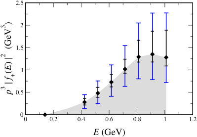
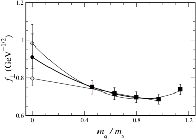
Figure 5: $B\to\pi l\nu$: (a) Integrand of Eq. (10). (b) Dependence of the form factor $f_{\perp}$ on the light quark mass, in the range $0.4m_{s}<m_{q}<1.2m_{s}$.

Uncertainties are still about 15–20% on $|V_{ub}|$. A strategy for reducing them are given in Ref. El-Khadra et al. (2001).

Ref. El-Khadra et al. (2001) finds strong dependence on the light quark mass, as illustrated for $f_{\perp}(0.7~{}\mathrm{GeV})$ in Fig. 5. This is the only calculation to reduce the light quark down to $m_{q}=0.4m_{s}$. The extrapolation to physical quark mass is the largest source of uncertainty quoted by Ref. El-Khadra et al. (2001), and a similar uncertainty is presumably present in all four calculations. One would like even lighter quarks, which take more CPU time.

Because of the discretization errors at higher $E$, the large light quark mass dependence, etc., a sanity check on $f_{+}(E)$ for $B\to\pi l\nu$ would be welcome. The calculation of similar form factors in $D$ decays encounters many of the same issues. A compelling test would be to compare lattice and experiment for $f_{+}^{D\to K}/f_{D_{s}}$ and $f_{+}^{D\to\pi}/f_{D}$, as a function of $E$. New physics is unlikely to alter the underlying processes, and the CKM matrix drops out. The CLEO-c program Briere et al. (2001) promises to measure these ratios with an uncertainty of a few percent.

3.3 $B\to D^{*}l\nu$ and $V_{cb}$

The exclusive semi-leptonic decay $B\to D^{*}l\nu$ is a good way to determine $|V_{cb}|$, but an estimate of the hadronic transition is needed. The differential decay rate is

$$\frac{d\Gamma}{dw}=\frac{G_{F}^{2}}{4\pi^{3}}\sqrt{w^{2}-1}m_{D^{*}}^{3}(m_{B}-m_{D^{*}})^{2}{\cal G}(w)|V_{cb}|^{2}|{\cal F}_{B\to D^{*}}(w)|^{2},$$ (11)

where $w=v\cdot v^{\prime}$ and ${\cal G}(1)=1$. At zero recoil ($w=1$) heavy-quark flavor symmetry forbids terms of order $1/m_{Q}$. The exclusive determination of $|V_{cb}|$ therefore proceeds by extracting $|V_{cb}{\cal F}_{B\to D^{*}}(1)|$ from a fit to the measurement of $d\Gamma/dw$, and then taking a theoretical estimate of ${\cal F}_{B\to D^{*}}(1)$. One would prefer the latter not to depend on models.

To see what is needed from the theoretical calculation, let us review the anatomy of ${\cal F}_{B\to D^{*}}(1)$. From HQET one can show that, at zero recoil,

$${\cal F}_{B\to D^{*}}(1)=\eta_{A}\left[1_{\mathrm{Isgur-Wise}}+0_{\mathrm{Luke}}/m+\delta_{1/m^{2}}+\delta_{1/m^{3}}\right]$$ (12)

where $\eta_{A}$ is a short-distance radiative correction, and the $\delta_{1/m^{n}}$ contain the long-distance properties of the bound states. The numerical values of $\eta_{A}$ and the $\delta_{1/m^{n}}$ depend on how HQET is renormalized. It is less important which renormalization scheme is chosen than it is to use the same scheme for both. The $1/m_{Q}^{n}$ corrections take the form

$$\delta_{1/m^{2}} = -\frac{\ell_{V}}{(2m_{c})^{2}}+\frac{2\ell_{A}}{(2m_{c})(2m_{b})}-\frac{\ell_{P}}{(2m_{b})^{2}},$$ (13)

$$\delta_{1/m^{3}} = -\frac{\ell_{V}^{(3)}}{(2m_{c})^{3}}+\frac{\ell_{A}^{(3)}\Sigma+\ell_{D}^{(3)}\Delta}{(2m_{c})(2m_{b})}-\frac{\ell_{P}^{(3)}}{(2m_{b})^{3}},$$ (14)

where $\Sigma=1/(2m_{c})+1/(2m_{b})$ and $\Delta=1/(2m_{c})-1/(2m_{b})$.

With brute force alone, a sufficiently precise calculation of ${\cal F}_{B\to D^{*}}(1)$ lies beyond reach. (See Ref. Hashimoto et al. (2001) for details.) Hashimoto et al. Hashimoto et al. (2001) have devised a method to extract all $\ell$s in Eq. (13) and all but $\ell_{D}^{(3)}$ in Eq. (14). The key is the heavy-quark mass dependence of three double ratios of matrix elements. As in Eqs. (12)–(14), HQET implies

$$\frac{\langle D|\bar{c}\gamma^{4}b|B\rangle\langle B|\bar{b}\gamma^{4}c|D\rangle}{\langle D|\bar{c}\gamma^{4}c|D\rangle\langle B|\bar{b}\gamma^{4}b|B\rangle} = \eta_{V}^{2}\left[1-\Delta^{2}\left(\ell_{P}+\ell^{(3)}_{P}\Sigma\right)\right]^{2},$$ (15)

$$\frac{\langle D^{*}|\bar{c}\gamma^{4}b|B^{*}\rangle\langle B^{*}|\bar{b}\gamma^{4}c|D^{*}\rangle}{\langle D^{*}|\bar{c}\gamma^{4}c|D^{*}\rangle\langle B^{*}|\bar{b}\gamma^{4}b|B^{*}\rangle} = \eta_{V}^{2}\left[1-\Delta^{2}\left(\ell_{V}+\ell^{(3)}_{V}\Sigma\right)\right]^{2},$$ (16)

$$\frac{\langle D^{*}|\bar{c}\gamma^{j}\gamma_{5}b|B\rangle\langle B^{*}|\bar{b}\gamma^{j}\gamma_{5}c|D\rangle}{\langle D^{*}|\bar{c}\gamma^{j}\gamma_{5}c|D\rangle\langle B^{*}|\bar{b}\gamma^{j}\gamma_{5}b|B\rangle} = \frac{\eta_{A^{cb}}\eta_{A^{bc}}}{\eta_{A^{cc}}\eta_{A^{bb}}}\left[1-\Delta^{2}\left(\ell_{A}+\ell^{(3)}_{A}\Sigma\right)\right]^{2}.$$ (17)

In particular, heavy-quark spin symmetry requires the same $\ell$s to appear in Eqs. (15)–(17) as in Eqs. (13) and (14).

In a lattice calculation of these double ratios most of the statistical and sytematic uncertainties cancel. The main difference from continuum QCD is that the short-distance coefficients are different Kronfeld (2000); Hashimoto et al. (2001). But, just like in continuum QCD, the short-distance behavior can be computed in perturbation theory. Thus, the analysis proceeds by removing the lattice short-distance contribution, fitting to the prediction of HQET, and then reconstituting $\mathcal{F}_{B\to D^{*}}(1)$ from the $\ell$s and $\eta_{A}$. The result is

$$\mathcal{F}_{B\to D^{*}}(1)=0.9??^{+0.024}_{-0.017}\pm 0.016{}^{+0.003}_{-0.014}{}^{+0.000}_{-0.016}{}^{+0.006}_{-0.014}.$$ (18)

To encourage the reader to think about the uncertainties, the central value is not revealed until the end. The error bars come from, in order, statistics and fitting, matching lattice gauge theory with HQET to QCD, lattice spacing dependence, light quark mass effects, and the quenched approximation. The secret to the small error on ${\cal F}$ is that they all scale as ${\cal F}-1$, by design. As a fraction of ${\cal F}-1$ the uncertainties are still sizable: 5–25%.

The most novel aspect of this analysis is how seriously it takes the idea of matching lattice gauge theory to QCD through HQET. A central part of the analysis is to calculate short-distance properties, which Ref. Hashimoto et al. (2001) does partly in perturbation theory. The second error bar reflects the associated uncertainty. It is reducible, but through traditional theoretical physics, rather than intensive computation.

4 An Octopus’s Garden

Although it does not bear directly the unitarity triangle, I would like to discuss some recent work by Nathan Isgur. I did not know Nathan well, but his enthusiasm for physics, especially the strong interactions, made a big impression on me. He struck me as the kind of person who had a hand all sorts of things. He must have needed eight arms to keep all his projects moving.

In the last year of his life, one of his projects was to understand whether instanton-like gauge fields or, on the other hand, disordered gauge fields play a larger role in QCD Isgur and Thacker (2001); Horvath et al. (2001); Bardeen et al. (2001). This work reflected Nathan’s broad knowledge of the phenomenological and theoretical sides of the strong interactions, touching on the OZI rule, chiral zero modes, the $\eta^{\prime}$ mass, instantons, the quark model, the AdS/CFT correspondence, lattice QCD, and the large $N_{c}$ limit. A particularly striking passage notes first how recent work by Witten on the AdS/CFT correspondance favors disordered, confining gauge fields (although those sentences were probably written by Nathan’s collaborator Hank Thacker), and then how details of how to treat strong decays in the quark model favor the disorder also. That part was certainly written by Nathan.

These issues surround the quantum ground state, or vacuum, of QCD. Gauge theories have many classical ground states, one for each integer. Instantons are the semi-classical configurations that tunnel from one ground state to another. In a quantum mechanical situation, fluctuation-dominated configurations could also mediate tunneling. Nathan proceeded by devising tests that could distinguish whether the quantum vacuum is obtained via such disordered gauge fields or via a gas or liquid of instantons. He then used (quenched) lattice QCD to see which way the gauge fields behaved.

One test stemmed from the observation, from empirically successful quark models of strong decays, that quark pairs pop out of the vacuum with scalar (i.e., ${}^{3}P_{0}$) quantum numbers. That implies that the OZI rule should fail for $J^{PC}=0^{++}$ quantum numbers. (The OZI rule says that decays, like $\phi\to\pi\pi$, in which quarks annihilate, are weaker than those, like $\phi\to KK$, in which they do not.) Empirically, the OZI rule fails in the $0^{-+}$ sector; that is how the $\eta^{\prime}$ mass is split away from the other pseudoscalar mesons. For the $0^{++}$ sector, however, there is a dearth of experimental data. Isgur and Thacker’s idea to to compute the quark annihilation process with lattice QCD, for various $J^{PC}$, which is possible at leading order in the OZI approximation even in quenched QCD Isgur and Thacker (2001). They found a small amplitude where the OZI rule holds empirically, e.g., for $J^{PC}=1^{-+}$. But for scalar and pseudoscalar channels the amplitude is large. This is evidence against an instanton-dominated vacuum, because instantons couple to quarks through the axial anomaly, that is, preferentially to the pseudoscalar channel.

5 Unblinding

Instead of a paragraph of bland conclusions, the reward for readers who have made it this far consists of the most interesting numerical results. The preliminary results of JLQCD on $B$ physics with $n_{f}=2$ are Yamada et al. (2001)

$$f_{B_{d}} = 190(14)(7)(19)~{}{\rm MeV},$$ (19)

$$f_{B_{s}}/f_{B_{d}} = 1.184(26)(20)(15),$$ (20)

$$\xi = 1.183(27)(20)(15),$$ (21)

where $\xi$ is a combination of their results for $f_{B_{s}}/f_{B_{d}}$ and $B_{B_{s}}/B_{B_{d}}$. In her review at Lattice ’01 Ryan (2001), Sinéad Ryan took stock of the ratio $\xi$, which enters into UT fits. Although JLQCD’s result is still preliminary, it cannot be denied that the chiral logarithms could affect $f_{B_{s}}/f_{B_{d}}$ and, hence, $\xi$. Ryan’s average, which strikes me as reasonable, is

$$\xi=1.15\pm 0.06^{+0.07}_{-0.00}$$ (22)

which retains the central value in common usage, but allows for a future upward revision, once the chiral behavior is fully understood and controlled.

For the zero-recoil form factor needed to determine $|V_{cb}|$ from $B\to D^{*}l\nu$, Ref. Hashimoto et al. (2001) finds

$${\cal F}_{B\to D^{*}}(1)=0.913^{+0.024}_{-0.017}{}^{+0.017}_{-0.030},$$ (23)

with systematics added in quadrature. Note that this result does not include the QED correction of +0.007, which is included, for example, in the BaBar Physics Book. This result still relies on the quenched approximation. Nevertheless, it is probably still under better control than estimates based on the quark model.

A hallmark of these two results, shared by some work on $B\to\pi l\nu$ for $|V_{ub}|$ El-Khadra et al. (2001); Aoki et al. (2001), is that they attempt a full analysis of the uncertainties, including those of heavy quarks, the chiral behavior, and quenching. Thus, they are suitable templates for the next round of lattice calculations, from which one can expect serious unquenched calculations with a direct impact on our knowledge of the unitarity triangle.

References

- Kronfeld (2001) Kronfeld, A. S., “ and mesons in lattice QCD”, in 30th International Conference on High-Energy Physics, edited by C. S. Lim and T. Yamanaka, World Scientific, 2001, hep-ph/0010074.
- Beneke (2001) Beneke, M., talk at XIX International Symposium on Lattice Field Theory, URL http://www.ifh.de/~latt2001/plenary-transp.html.
- Ali Khan (2000) Ali Khan, A., et al. [CP-PACS Collaboration], Phys. Rev. D 64, 034505 (2001) [hep-lat/0010009].
- Ali Khan (2000) Ali Khan, A., et al. [CP-PACS Collaboration], Phys. Rev. D 64, 054504 (2001) [hep-lat/0103020].
- Bernard (2001) Bernard, C., et al., Nucl. Phys. Proc. Suppl. 94, 346 (2001) [hep-lat/0011029]; hep-lat/0110072.
- Sexton and Weingarten (1997) Sexton, J., and Weingarten, D., Phys. Rev. D55, 4025 (1997).
- Morel (1987) Morel, A., J. Phys. (France) 48, 1111 (1987).
- Sharpe (1990) Sharpe, S. R., Phys. Rev. D41, 3233 (1990).
- Bernard and Golterman (1992) Bernard, C. W., and Golterman, M. F. L., Phys. Rev. D46, 853 (1992) [hep-lat/9204007].
- Bernard and Golterman (1994) Bernard, C. W., and Golterman, M. F. L., Phys. Rev. D49, 486 (1994) [hep-lat/9306005].
- Bardeen et al. (2001) Bardeen, W., Duncan, A., Eichten, E., Isgur, N., and Thacker, H., hep-lat/0106008.
- Symanzik (1983a) Symanzik, K., Nucl. Phys. B226, 187 (1983a); 205 (1983b).
- Eichten (1988) Eichten, E., “Heavy Quarks on the Lattice”, in Field Theory on the Lattice, edited by A. Billoire et al., North-Holland, 1988.
- Eichten and Hill (1990) Eichten, E., and Hill, B., Phys. Lett. B234, 511 (1990).
-
Lepage and Thacker (1988)
Caswell, W. E., and Lepage, G. P.,
Phys. Lett. B 167, 437 (1986);
Lepage, G. P., and Thacker, B. A., “Effective Lagrangians for Simulating Heavy Quark Systems”, in Field Theory on the Lattice, edited by A. Billoire et al., North-Holland, 1988. - Thacker and Lepage (1991) Thacker, B. A., and Lepage, G. P., Phys. Rev. D43, 196 (1991).
- El-Khadra et al. (1997) El-Khadra, A. X., Kronfeld, A. S., and Mackenzie, P. B., Phys. Rev. D55, 3933 (1997) [hep-lat/9604004].
- Kronfeld (2000) Kronfeld, A. S., Phys. Rev. D62, 014505 (2000) [hep-lat/0002008].
- Yamada et al. (2001) Yamada, N., et al. [JLQCD Collaboration], hep-lat/0110087.
- Sharpe and Zhang (1996) Sharpe, S. R., and Zhang, Y., Phys. Rev. D53, 5125 (1996) [hep-lat/9510037].
- Anastassov et al. (2001) Anastassov, A., et al. [CLEO Collaboration], hep-ex/0108043.
- Bowler et al. (2000) Bowler, K. C., et al. [UKQCD Collaboration], Phys. Lett. B486, 111 (2000) [hep-lat/9911011].
- Abada et al. (2000) Abada, A., et al., hep-lat/0011065.
- El-Khadra et al. (2001) El-Khadra, A. X., Kronfeld, A. S., Mackenzie, P. B., Ryan, S. M., and Simone, J. N., Phys. Rev. D64, 014502 (2001) [hep-ph/0101023].
- Aoki et al. (2001) Aoki, S., et al. [JLQCD Collaboration], Phys. Rev. D64, 114505 (2001) [hep-lat/0106024].
-
Briere et al. (2001)
Briere, R. A., et al.,
“CLEO-c and CESR-c: A New Frontier of Weak and Strong
Interactions”,
CLNS-01-1742;
Shipsey, I. P. J., these proceedings. - Hashimoto et al. (2001) Hashimoto, S., Kronfeld, A. S., Mackenzie, P. B., Ryan, S. M., and Simone, J. N., hep-ph/0110253.
- Isgur and Thacker (2001) Isgur, N., and Thacker, H. B., Phys. Rev. D64, 094507 (2001) [hep-lat/0005006].
- Horvath et al. (2001) Horvath, I., Isgur, N., McCune, J., and Thacker, H. B., hep-lat/0102003.
- Ryan (2001) Ryan, S., hep-lat/0111010.