XXX-XXXXX YYY-YYYYYY

Are Heavy Particles Boltzmann Suppressed?

Patrizia Bucci

Department of Physics, University of Padova,
Via F. Marzolo 8, I-35131 Padova, Italy.
Institute of Theoretical Physics,
University of Warsaw,
ul. Hoza 69,PL-00-681, Warsaw, Poland.

and

Massimo Pietroni

INFN - Sezione di Padova,
Via F. Marzolo 8, I-35131 Padova, Italy

Matsumoto and Yoshimura have recently argued that the number density of heavy particles in a thermal bath is not necessarily Boltzmann-suppressed for $T\ll M$, as power law corrections may emerge at higher orders in perturbation theory. This fact might have important implications on the determination of WIMP relic densities. On the other hand, the definition of number densities in a interacting theory is not a straightforward procedure. It usually requires renormalization of composite operators and operator mixing, which obscure the physical interpretation of the computed thermal average. We propose a new definition for the thermal average of a composite operator, which does not require any new renormalization counterterm and is thus free from such ambiguities. Applying this definition to the annihilation model of Matsumoto and Yoshimura we find that it gives number densities which are Boltzmann-suppressed at any order in perturbation theory. We discuss also heavy particles which are unstable already at $T=0$, showing that power law corrections do in general emerge in this case.

PRESENTED BY P. BUCCI AT

COSMO-01
Rovaniemi, Finland,
August 29 – September 4, 2001

1 Introduction

The computation of number density of cosmological relics, such as weakly interacting heavy particles (WIMPs), neutrinos etc is usually realized by using a thermally average Boltzmann equation [1, 2]. The scenario which emerges is that of a sudden freeze-out: the particle number density follows the equilibrium value until the freeze-out temperature below which the annihilation is frozen. The freeze-out temperature of pair annihilation model may roughly be estimated by equating the annihilation rate to the Hubble rate, the relic abundance is then computed by the thermal number density at that freeze-out temperature, thus, we expect it is Boltzmann suppressed if the freeze-out temperature ($T_{f}$) is much smaller than the mass of the particle. This is the typical case for a WIMP: the freeze-out temperature is typically 4-5 $\%$ of the mass of the particle namely, they are non relativistic at decoupling, and their annihilation cross section is of the right order to give a contribution to $\Omega_{M}$ of order unity, so that they are very good candidates for cold dark matter models [3].
But from recent papers [4], Matsumoto and Yoshimura (MY) have challenged the above conventional conclusion, claiming that two-loop corrections to the number density exhibit only power-law suppression in $T_{f}/M$, thus dominating over the Boltzmann-suppressed tree-level contribution if $T_{f}$ is low enough. If confirmed, such a finding would imply that the present constraints on dark matter models are actually underestimated and should be carefully reconsidered. To be definite, MY introduced a toy model of two real scalar fields with Lagrangian

$${\cal L} = \mbox{\small$\frac{1}{2}$}\partial_{\mu}\phi\partial^{\mu}\phi-\mbox{\small$\frac{1}{2}$}M^{2}\phi^{2}-\frac{\lambda_{\phi}}{4!}\phi^{4}+\mbox{\small$\frac{1}{2}$}\partial_{\mu}\chi\partial^{\mu}\chi-\mbox{\small$\frac{1}{2}$}m^{2}\chi^{2}$$ (1)

$$-\frac{\lambda_{\chi}}{4!}\chi^{4}-\frac{\lambda}{4}\phi^{2}\chi^{2}\,,$$

with $M\gg m$. The following relations were assumed among the coupling constants

$$|\lambda_{\phi}|\ll\lambda^{2}\,,\;\;\;\;\;\;|\lambda|\ll|\lambda_{\chi}|<1\,,$$

so that the light $\chi$ particles act as an efficient heat bath for the heavy $\phi$’s. They then considered the quadratic part of the Hamiltonian for $\phi$,

$$H_{\phi}=\mbox{\small$\frac{1}{2}$}\dot{\phi}^{2}+\mbox{\small$\frac{1}{2}$}(\nabla\phi)^{2}+\mbox{\small$\frac{1}{2}$}M^{2}\phi^{2}\,,$$ (2)

and, for temperatures $T$ such that $m\ll T\ll M$ they defined the number density of $\phi$ particles as

$$N_{\phi}=\frac{\langle H_{\phi}+{\mathrm{c}ounterterms}\rangle_{T}}{M}\,\$$ (3)

where MY define the thermal average for an operator $A$ as

$$\langle A\rangle_{T}\equiv\frac{\mathop{\mathrm{tr}}Ae^{-H/T}}{\mathop{\mathrm{tr}}e^{-H/T}}-\frac{\langle 0|A|0\rangle}{\langle 0|0\rangle},$$ (4)

$H$ being the total Hamiltonian. At tree-level, the well known Boltzmann-suppressed contribution is obtained

$$N_{\phi}^{(0)}=\left(\frac{MT}{2\pi}\right)^{3/2}e^{-M/T}\,.$$

The power-law contribution arises at two-loops and is given by

$$N_{\phi}^{(2)}=c\lambda^{2}\frac{T^{6}}{M^{3}},\,\,\,\,\,\,\,\,\,c=\frac{1}{69120}\,$$ (5)

While in the standard case the contribution to $\Omega_{M}$ depends on the mass of the particle only trough logarithmic terms, in this case, with the different power law behavior (5), a simple calculation shows that the energy density goes like $\sim M^{1/4}$, implying much stronger constraints on the mass of the particle. The interpretation of (3) as the physical number density of heavy $\phi$ particles has been questioned by several authors [5, 6, 7]: what emerges from all these papers is that the real problem is the definition of the number density for a heavy particle in a interacting theory. We will show that it is possible to give a non-ambiguous definition of the number density of an interacting particle at any temperature and at any order in perturbation theory. In the case of the MY model of eq. (1), our definition exhibits the expected Boltzmann-suppression at low temperature. We will find it very convenient to work in the real-time formalism of finite temperature field theory (RTF) [8], which has the advantage of keeping $T=0$ and finite temperature effects well separated. Indeed, as we will discuss, the ambiguities in the conventional definitions of the number density are mostly due to the $T=0$-renormalization procedure. Being able to single out $T=0$ ultraviolet (UV) divergences turns then out to be a great advantage when one is interested in genuine thermal effects. The tree-level propagator for a real scalar particle in the RTF has the structure:

$${\bf D_{0}}={\bf D_{0}^{T=0}}+{\bf D_{0}^{T}}=i{\bf P[}\Delta_{0}{\bf]}+i(\Delta_{0}-\Delta_{0}^{*}){\cal N}(|q_{0}|){\bf B}\,,$$ (6)

where $\Delta_{0}^{(*)}=(q^{2}-M^{2}+(-)i\varepsilon)^{-1}$ is the tree-level Feynman propagator, ${\cal N}$ the Bose-Einstein (Fermi-Dirac) distribution function, ${\cal N}(x)=(\exp(x/T)-(+)1)^{-1}$ and the two matrices ${\bf P}$ and ${\bf B}$ are defined as

$${\bf P[}a(q){\bf]} = \left[\begin{array}[]{cc}a(q)&(a-a^{*})(q)\theta(-q_{0})\\ &\\ (a-a^{*})(q)\theta(q_{0})&-a^{*}(q)\end{array}\right]\,\,,$$ (10)

$${\bf B} = \left[\begin{array}[]{cc}1&1\\ 1&1\end{array}\right],$$ (13)

with $\theta(x)$ the Heaviside’s step function.

The full propagator has the same structure as the tree-level one, eq. (6), with $\Delta_{0}^{(*)}$ replaced by its all-order counterpart [8]

$$\Delta^{(*)}(q)=\frac{1}{q^{2}-M^{2}-\Pi(q_{0},|\vec{q}|)+(-)i\varepsilon}\,\,,$$ (15)

$\Pi(q_{0},|\vec{q}|)$ being the (renormalized) full self-energy at finite temperature. In the following, we will refer to $i{\bf P}[\Delta_{0}]$ and $i{\bf P}[\Delta]$ as the “$T=0$” parts of the tree-level and full propagators, and to $i(\Delta_{0}-\Delta_{0}^{*}){\cal N}(|q_{0}|){\bf B}$ and $i(\Delta-\Delta^{*}){\cal N}(|q_{0}|){\bf B}$ as the “thermal” parts. It is important to notice that what we call the “$T=0$” part of the full propagator actually contains thermal corrections in the self-energy, so it is not the full $T=0$ propagator.
The report presented here is a summary of our recent work [9].

2 Renormalization of $\phi_{0}^{2}$

Definition of number density generally comes out from bilinear operators (see (3) for MY model ), thus, we have to study composite operator renormalization. They arise when we consider local product of fields making up the operator. New UV divergences are induced when it is inserted in a Green function, which are generally not canceled by the Lagrangian counterterms. The renormalization of these divergences then requires the introduction of new counterterms. Renormalized operators can be defined, which are generically expressible as linear combinations of all the bare operators of equal or lower canonical dimensionality (for a thorough discussion of composite operator renormalization, see for instance [10, 11]). Before considering the complete energy-momentum tensor, the analysis of the composite operator $\phi_{0}^{2}$ (where the $0$-label indicates the bare fields, masses and coupling constants) will be useful in illustrating the main points of renormalization and thermal averaging. We start by considering the $T=0$ case. In the model (1) the renormalization of $\phi_{0}^{2}$ then induces a mixing with $\chi_{0}^{2}$, and the two renormalized operators, $[\phi^{2}]$ and $[\chi^{2}]$ can be expressed as

$$\left(\begin{array}[]{l}\displaystyle[\phi^{2}]\\ \displaystyle[\chi^{2}]\end{array}\right)=\left(\begin{array}[]{cc}1-\delta Z_{\phi\phi}&\delta Z_{\phi\chi}\\ \delta Z_{\chi\phi}&1-\delta Z_{\chi\chi}\end{array}\right)\left(\begin{array}[]{l}\phi_{0}^{2}\\ \chi_{0}^{2}\end{array}\right)\,.$$ (16)

In minimal-subtraction scheme (MS) the bare parameters can be expressed in terms of the renormalized ones as

$$\lambda_{i,0}=\mu^{4-D}\lambda_{i}\left(1+\sum_{k=1}^{\infty}\frac{a_{k}^{i}(\{\lambda_{j}\};D)}{(D-4)^{k}}\right)\,,$$

$$M_{0}^{2}=M^{2}\left(1+\frac{\delta M^{2}}{M^{2}}\right)=M^{2}\left(1+\frac{\mu^{2}}{M^{2}}\sum_{k=1}^{\infty}\frac{b_{k}^{M}(\{\lambda_{j}\};D)}{(D-4)^{k}}\right)\,,$$

$$m_{0}^{2}=m^{2}\left(1+\frac{\delta m^{2}}{m^{2}}\right)=m^{2}\left(1+\frac{\mu^{2}}{m^{2}}\sum_{k=1}^{\infty}\frac{b_{k}^{m}(\{\lambda_{j}\};D)}{(D-4)^{k}}\right)\,,$$ (17)

where $\{\lambda_{i}\}=\{\lambda_{\phi},\lambda_{\chi},\lambda\}$, $D$ is the space-time dimensionality, and the important point is that the $a_{k}^{i}$’s, $b_{k}^{M}$’s and $b_{k}^{m}$’s are mass, momentum, and temperature independent. Using eqs. (17) it is then possible to prove that, for any renormalized green function $G$ the following relation holds

$$M_{0}^{2}\frac{\partial G}{\partial M_{0}^{2}}+m_{0}^{2}\frac{\partial G}{\partial m_{0}^{2}}=M^{2}\frac{\partial G}{\partial M^{2}}+m^{2}\frac{\partial G}{\partial m^{2}}\,,$$

showing that, being the right hand side manifestly finite, the insertion of the combination $M_{0}^{2}\phi_{0}^{2}+m_{0}^{2}\chi_{0}^{2}$ does not induce any UV divergence. The $\delta Z_{\phi\phi}$, $\delta Z_{\chi\chi}$ renormalization constants can then be expressed in terms of the mass counterterms as

$$\left\{\begin{array}[]{c}\displaystyle\delta Z_{\phi\phi}=\displaystyle-\frac{\delta M^{2}}{M^{2}}-\frac{m^{2}}{M^{2}}\delta Z_{\chi\phi}\\ \displaystyle\delta Z_{\chi\chi}=-\frac{\delta m^{2}}{m^{2}}-\frac{M^{2}}{m^{2}}\delta Z_{\phi\chi}\end{array}\right.$$ (18)

whereas the remaining counterterms $\delta Z_{\phi\chi}$, $\delta Z_{\chi\phi}$, can be computed as

$$\delta Z_{\phi\chi} = \displaystyle-\left.\frac{\langle\phi_{0}^{2}(x)\chi(y)\chi(z)\rangle}{\langle\chi_{0}^{2}(x)\chi(y)\chi(z)\rangle}\right|_{\mathrm{D}IV}\,,\,\,\,\,\,$$

$$\delta Z_{\chi\phi} = \displaystyle-\left.\frac{\langle\chi_{0}^{2}(x)\phi(y)\phi(z)\rangle}{\langle\phi_{0}^{2}(x)\phi(y)\phi(z)\rangle}\right|_{\mathrm{D}IV}\,.$$

3 Thermal average without mixing

The mixing between the $\phi^{2}$ and $\chi^{2}$ operator makes the definition of a pure $\phi$-number density quite cumbersome. A diagrammatic analysis can help us in identifying the $T=0$ nature of the pollution by the $\chi$ field so that we can give a definition of thermal expectation value for $\phi^{2}$ which is free from it. Let us consider $\mathop{\mathrm{tr}}e^{-H/T}[\phi^{2}]/\mathop{\mathrm{tr}}e^{-H/T}$. At tree-level in the RTF it is given by the two diagrams in fig. 1a

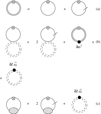
Figure 1: Diagrammatic expansion of $\langle[\phi^{2}]\rangle_{T}$.

where the continuous line represents the $T=0$ part of the $\phi$ propagator, the barred continuous line the thermal part and the double line the sum of the two. The first diagram is quadratically divergent and requires a subtraction, whereas the second one, thanks to the Bose-Einstein function contained in ${\bf D_{0}^{T}}(q)$, is finite. At $O(\lambda)$ the diagrams of fig. 1b contribute. There are also contributions $O(\lambda_{\phi})$ (such as higher order contributions containing also $\lambda_{\chi}$) but their consideration is not necessary for our discussion, so we will limit ourselves to contributions containing only powers of $\lambda$. The (quadratic) divergence due to the $T=0$ $\chi$-tadpole diagram (dashed line) is canceled by the mass counterterm. The only remaining divergence comes from the first diagram, in which both the $\phi$ lines, entering the cross are of $T=0$ type. It is the cancellation of this divergence which calls into play the mixing, via the renormalization constant $\delta Z_{\phi\chi}$ appearing in the last diagram.
At $O(\lambda^{2})$ (fig. 1c) the same happens, where:

is the self energy to $O(\lambda^{2})$ renormalized by Lagrangian counterterms. The last diagram, containing a tree-level $\chi^{2}$ operator multiplied by a $O(\lambda^{2})$ renormalization constant is required in order to cancel the divergence coming from the integration over the momentum of $\phi$ particles flowing to the cross with $T=0$ propagators (the first diagram in fig. 1c). Note that, due to the general relation $\sum_{i,j=1,2}\Sigma_{ij}=0$, $\Sigma_{ij}$ being the self-energy with external thermal indices $i$ and $j$, the contribution with both lines of thermal type also vanishes, once the summation over thermal indices is taken. The remaining loop divergences are canceled by usual Lagrangian counterterms and therefore require no mixing. The only divergence which is not canceled by neither Lagrangian nor composite operators counterterms is the tree-level one. Then, one usually defines the thermal expectation value of $\phi^{2}$ as the expectation value of $[\phi^{2}]$ subtracted according to one of the two following ways [8, 12],

$$\langle[\phi^{2}]\rangle_{T} \equiv \frac{\mathop{\mathrm{tr}}[\phi^{2}]e^{-H/T}}{\mathop{\mathrm{tr}}e^{-H/T}}-\frac{\langle 0|[\phi^{2}]|0\rangle}{\langle 0|0\rangle}\,\,\,\,\,\,\,\,\,\,\,\,\,\,\,{\mathrm{o}r}$$ (19)

$$\equiv \frac{\mathop{\mathrm{tr}}[\phi^{2}]e^{-H/T}}{\mathop{\mathrm{tr}}e^{-H/T}}-\left.\frac{\langle 0|[\phi^{2}]|0\rangle}{\langle 0|0\rangle}\right|_{\mathrm{f}reefields}\,\,\,\,\,\,\,\,\,\,\,\,\,\,\,.$$

The definitions above are both finite, and thus a plausible choice. However, both of them include the contributions from the first and the last graphs in figs. 1b and 1c, that is, they require mixing.

The above analysis suggests a new definition of thermal average of $\phi^{2}$, which represents the main point of this paper, namely

$$\langle\phi^{2}\rangle_{\mathrm{T}h} \equiv \int\frac{d^{4}q}{(2\pi)^{4}}D^{T}(q)$$ (20)

$$= \int\frac{d^{4}q}{(2\pi)^{4}}i(\Delta-\Delta^{*})(q){\cal N}(|q_{0}|)\,\,\,\,,$$

where $D^{T}(q)$ is any of the four component of the thermal part of the full propagator.

Expanding $\Delta^{(*)}$ as $\Delta^{(*)}=\Delta_{0}^{(*)}+\Delta_{0}^{(*)}\Pi\Delta_{0}^{(*)}+\dots$, and recalling the relations between $\Pi(q_{0},|\vec{q}|)$ and $\Sigma(q_{0},|\vec{q}|)_{ij}$ [8],

$$\mathop{\mathrm{Re}}\Pi(q)=\mathop{\mathrm{Re}}\Sigma_{11}(q)\,,\,\,\,\,\,\,\,\,\mathop{\mathrm{Im}}\Pi(q)=\varepsilon(q_{0})\mathop{\mathrm{Im}}\left[\Sigma_{11}(q)+\Sigma_{12}(q)\right]\,,$$

one can check that the perturbative expansion of fig. 1 is reproduced, apart from the ‘problematic’ diagrams. The definition in (20) then automatically gets rid of all the unpleasant features of the conventional definitions in eq. (19), namely, the need of an arbitrary subtraction and, more importantly, composite operator renormalization and mixing.

4 Averaging the energy-momentum tensor

The renormalization of the energy-momentum tensor is discussed in refs.[8, 11, 12]. Expressing it in terms of bare parameters, the operator

$$T^{\mu\nu}=\partial^{\mu}\phi_{0}\partial^{\nu}\phi_{0}+\partial^{\mu}\chi_{0}\partial^{\nu}\chi_{0}-g^{\mu\nu}{\cal L}_{0}+\cdots\,,$$

is finite when inserted in a Green function, that is, it does not require extra counterterms besides those already present in the Lagrangian. The dots in the formula above represent pole terms proportional to $(\partial^{\mu}\partial^{\nu}-g^{\mu\nu}\partial^{2})\phi_{0}^{2}$ and to $(\partial^{\mu}\partial^{\nu}-g^{\mu\nu}\partial^{2})\chi_{0}^{2}$. Since we are interested in the thermal average of $T^{\mu\nu}$ alone, translation invariance insures that such pole terms do not contribute. On the other hand, a subtraction of the $T=0$ contribution as in eqs. (19) is needed. Working with renormalized parameters, $T^{\mu\nu}$ is expressed as

$$T^{\mu\nu}=T^{\mu\nu}_{\mathrm{c}an}+T^{\mu\nu}_{\mathrm{c}.t.}\,,$$ (21)

where $T^{\mu\nu}_{\mathrm{c}an}$ has the canonical form and $T^{\mu\nu}_{\mathrm{c}.t.}$ contains only the Lagrangian counterterms.

The finiteness of $T^{\mu\nu}$ means that the divergences induced by, e.g., the composite operator $\phi^{2}\chi^{2}$ are canceled by the Lagrangian counterterms and the particular combination of operators $\phi^{4}$, $\chi^{4}$, $(\partial\phi)^{2},\ldots$, appearing in $T^{\mu\nu}$. In general, if we split $T^{\mu\nu}$ in parts, each part separately will require composite operator renormalization. Indeed, this is what is done by MY in ref. [4]. They split the total Hamiltonian as

$$T^{00}\equiv H_{\mathrm{t}ot}=H_{\phi}+H_{\chi}+H_{\mathrm{i}nt}+H_{\mathrm{c}.t.}\,,$$

and compute thermal average of $H_{\phi}$ (given in eq. (2)). In the RTF it gives

$$\frac{\mathop{\mathrm{tr}}H_{\phi}e^{-H/T}}{\mathop{\mathrm{tr}}e^{-H/T}} = \mbox{\small$\frac{1}{2}$}\int\frac{d^{4}q}{(2\pi)^{4}}\left[2q_{0}^{2}-(q^{2}-M^{2})\right]\cdot$$ (22)

$$\,\,\,\,\,\,\,\,\,\,\,\,\cdot[{\bf D^{T=0}}+{\bf D^{T}}]_{12}(q)]\,,$$

where, differently from eq. (20), also the $T=0$ part of the full propagator appears. It is important to recall here what we have noticed after eq.(15), namely that the $T=0$ full propagator contains thermal effects via the self-energy. Such contributions are not canceled by purely $T=0$ subtractions like those defined in eq. (19). By perturbatively expanding $[{\bf D^{T=0}}]_{12}$ in (22) at $O(\lambda^{2})$ we find, apart from divergent contributions which require composite operator counterterms to be added to $H_{\phi}$, the “famous” power-law contribution

$$\begin{array}[]{l}\displaystyle\mbox{\small$\frac{1}{2}$}\int\frac{d^{4}q}{(2\pi)^{4}}\left[2q_{0}^{2}-(q^{2}-M^{2})\right]\left.[{\bf D^{T=0}}]_{12}(q)\right|_{O(\lambda^{2})}=\\ \displaystyle\mbox{\small$\frac{1}{2}$}\int\frac{d^{4}q}{(2\pi)^{4}}\left[2q_{0}^{2}-(q^{2}-M^{2})\right]\theta(-q_{0})\\ \displaystyle\left[i(\Delta_{0}^{2}-{\Delta_{0}^{*}}^{2})\mathop{\mathrm{Re}}\Pi-(\Delta_{0}^{2}+{\Delta_{0}^{*}}^{2})\epsilon(q_{0})\mathop{\mathrm{Im}}\Pi\right]\\ \displaystyle={\mathrm{d}iv.}+\frac{1}{69120}\frac{\lambda^{2}T^{6}}{M^{2}}+\cdots\,\,,\end{array}$$ (23)

where $\epsilon(q_{0})\equiv\theta(q_{0})-\theta(-q_{0})$. The same contribution, with opposite sign, is found from the corresponding piece of the thermal average for $H_{\chi}$.

Paralleling our discussion in the previous section, we will instead define the energy density of the $\phi$ field as

$$\rho_{\phi}^{\prime}\equiv\mbox{\small$\frac{1}{2}$}\int\frac{d^{4}q}{(2\pi)^{4}}\left[2q_{0}^{2}-(q^{2}-M^{2})\right][{\bf D^{T}}]_{12}(q)\,,$$ (24)

and analogously for $\rho_{\chi}^{\prime}$. The complete energy density will then be split as

$$\rho_{\mathrm{t}ot}\equiv\langle H_{\mathrm{t}ot}\rangle_{T} \equiv \frac{\mathop{\mathrm{tr}}H_{\mathrm{t}ot}e^{-H/T}}{\mathop{\mathrm{tr}}e^{-H/T}}-\frac{\langle 0|H_{\mathrm{t}ot}|0\rangle}{\langle 0|0\rangle}$$ (25)

$$=\rho_{\phi}^{\prime}+\rho_{\chi}^{\prime}+\rho_{\mathrm{i}nt}^{\prime}\,,$$

so that the contribution of eq. (23) enters $\rho_{\mathrm{i}nt}^{\prime}$ instead of $\rho_{\phi}^{\prime}$. Notice that neither $\rho_{\phi}^{\prime}$ nor $\rho_{\chi}^{\prime}$ are affected by the $T=0$ subtraction.

The definition in (25) exhibits three remarkable properties:

i) The splitting in (25) is closed under operator mixing and composite operator renormalization. No composite operator counterterm is required to make $\rho_{\phi}^{\prime}$ or $\rho_{\chi}^{\prime}$ separately finite and, since $\rho_{\mathrm{t}ot}$ is also finite, the same is true also for $\rho_{\mathrm{i}nt}^{\prime}$. Thus, our definition of number density, differently from that considered by MY, is independent on the renormalization scale $\mu$ . There is no “pollution” from $\rho_{\chi}^{\prime}$ to $\rho_{\phi}^{\prime}$ at any value of $\mu$.

ii) None of the three pieces in (25) contains $O(\lambda^{2}T^{6}/M^{2})$ terms. Indeed, the contribution of eq. (23) and the analogous one for the $\chi$’s go both into $\rho_{int}^{\prime}$ and there, because of their opposite sign, cancel.

iii) $\rho_{\phi}^{\prime}$ is Boltzmann-suppressed for $T\ll M$.Indeed, writing $[{\bf D^{T}}]_{12}(q)$ explicitly

$$[{\bf D^{T}}]_{12}(q)=-\frac{2\mathop{\mathrm{Im}}\Pi(q)\epsilon(q_{0})}{(q^{2}-M^{2}-\mathop{\mathrm{Re}}\Pi(q))^{2}+\mathop{\mathrm{Im}}\Pi(q)^{2}}{\cal N}(|q_{0}|)\,,$$ (26)

we see that, due to the Bose-Einstein function, non-Boltzmann-suppressed contributions to the integral in eq. (24) might only come from momenta $|q_{0}|\mathrel{\vbox{\hbox{$<$}\nointerlineskip\hbox{$\sim$}}}T\;(\ll M)$. But, for these values of momenta, it is the imaginary part of the self-energy (Figure 2) which is Boltzmann-suppressed.

Figure 2: Two-loop contribution to the self energy .

It can be easily understood looking at Figure 3 :

Figure 3: a) Decay, b) Annihilation, c) Landau damping .

for $|q_{0}|\mathrel{\vbox{\hbox{$<$}\nointerlineskip\hbox{$\sim$}}}T(\ll M)$ only the annihilation and the Landau damping contribute. In the former case (fig. 3.b) the on-shell $\phi$ particle in the initial state comes from the heat-bath and then carries a ${\cal N}$ factor. In the Landau damping case (fig. 3.c), the energy to create the on-shell $\phi$ has to be provided by the $\chi$ from the heat bath, so that a Boltzmann-suppressed ${\cal N}$ has to be payed in this case too.

5 A Better Definition for $N_{\phi}$

Using the $\phi$-energy density as given in eq. (24), we can now define the $\phi$ number density for $T\ll M$ in a way analogous to MY’s definition, eq. (3), that is

$$N_{\phi}=\frac{\rho_{\phi}^{\prime}}{M}\;\;\;\;{\mathrm{f}or\;\;\;T\ll M}\;.$$

However a better definition, valid at any value of $T$, and again based on the average of a quadratic operator, can be given as

$$N_{\phi}\equiv\int\frac{d^{4}q}{(2\pi)^{4}}|q_{0}|[{\bf D^{T}}]_{12}(q)\,.$$ (27)

As $\rho_{\phi}^{\prime}$, eq. (27) exhibits the nice features of not requiring composite operator renormalization and of being Boltzmann-suppressed at low temperatures, but in addition it may be extended to high temperatures or, equivalently, to the massless limit. The origin of eq. (27) can be derived in analogy to the case of a complex scalar field, $\Phi$, in case an exact $U(1)$ symmetry is imposed to the theory. The number density for the real scalar field $\phi$ should differ from the previous quantity in two respects. First, particle and antiparticle contributions should be summed up, in order to account for their ‘Majorana’ nature. This is obtained by taking the modulus of $|q_{0}|$ inside (27). Second, a factor $1/2$ is needed, in order to take into account the number of degrees of freedom.

6 The Decaying Case.

The discussion of the previous sections is straightforwardly generalizable to any model in which heavy particles annihilate into lighter ones, both bosons and fermions. The basic conclusions remain unalterated, the main reason being the Boltzmann-suppression of the imaginary part of the self-energy at small momenta.

The situation changes drastically if the heavy particle is unstable at $T=0$. If, for definiteness, it decays into two lighter particles of mass $m<M/2$ the propagator exhibits an imaginary part for $2m<p_{0}<M$ already at $T=0$, so that there is no reason to expect that it is Boltzmann-suppressed for $T<M$. The heavy particle is actually a resonance, whose energy-momentum can take values much lower than the peak at $p^{2}=M^{2}$, of course paying the usual Breit-Wigner suppression far away from the peak. In this case, power-law contributions to the resonance number density do in general emerge, as we will briefly discuss.

We will consider for definiteness the annihilation model discussed in ref. [13] and in the first of refs. [4], in which the interaction between the heavy $\Phi$ and the light $\chi$-bosons is due to the term

$${\cal L}_{\mathrm{i}nt}=-\frac{\mu}{2}\Phi\chi^{2}\,,$$ (28)

where we assume that $\mu\ll M$. In this model, the imaginary part of the self-energy is $\propto\mu^{2}$, so that, using (26) in (27) we get

$$N_{\Phi}\sim\frac{\Gamma_{0}}{M^{3}}T^{5}\,,$$ (29)

with $\Gamma_{0}\equiv\mu^{2}/(32\pi M)$ the $T=0$ decay rate on-shell. In ref. [13] a different behavior, $N_{\Phi}\sim T^{4}$ was claimed. Indeed, the following argument clarifies the physical origin of the power-law contribution and confirms the $T^{5}$ behavior.

In the thermal bath, unstable $\Phi$ particles are continuously produced in $\chi$-$\chi$ annihilations. Being the $\Phi$ a resonance, the production energy, $\omega$, can be much smaller than $M$. The produced $\Phi$’s eventually decay with inverse lifetime $\Gamma=\mu^{2}/(32\pi\omega)=\Gamma_{0}M/\omega$. Thus, the number density of $\Phi$’s of energy around $\omega$, $n^{\Phi}(\omega)$, obeys the rate equation

$$\frac{dn^{\Phi}(\omega)}{dt}=\gamma-\Gamma n^{\Phi}(\omega)\,,$$ (30)

where $\gamma$ is the rate per unit volume of the process

$$\chi\chi\rightarrow\Phi\rightarrow{\mathrm{e}verything}\;.$$ (31)

The above equation leads to the equilibrium value

$$n^{\Phi}_{\mathrm{e}q}(\omega)=\frac{\gamma}{\Gamma}\,.$$

The production rate is given by $\gamma\sim N_{\chi}^{2}\sigma v$, where the inclusive cross section $\sigma$ may be computed using the optical theorem as $\sigma\sim\mu^{2}\mathop{\mathrm{Im}}\Delta_{\Phi}/s$, $s$ being the square of the $\Phi$ four-momentum, and $\Delta_{\Phi}$ the full $\Phi$ propagator.

Taking $m\ll\sqrt{s}\sim T\ll M$, the initial $\chi$ particles are relativistic (i.e. $N_{\chi}\sim T^{3}$) and we get $\sigma\sim\mu^{4}/(M^{4}T^{2})$. Putting all together, we get a contribution to the total $\Phi$-number density from the region $\omega\sim T$ of order

$$n^{\Phi}_{\mathrm{e}q}(\omega\sim T)\sim\frac{\mu^{2}}{M^{4}}T^{5}\sim\frac{\Gamma_{0}}{M^{3}}T^{5}\,.$$ (32)

The $\Phi$’s with energies closer to the peak of the resonance live longer but their contribution to the number density is Boltzmann-suppressed, as two highly energetic $\chi$’s are required in the initial state to produce them.

As the energy of the relevant $\Phi$’s is typically $O(T)$, the energy density is

$$\rho_{\Phi}\sim O\left(\frac{\Gamma_{0}}{M^{3}}T^{6}\right)+{\mathrm{`}Boltzmann-suppressed^{\prime}}\,,$$

and $\rho_{\Phi}/\rho_{\chi}$ vanishes as $T^{2}$ at low temperatures. Before concluding this section, we observe that the definition of a sensible number density along the lines of eq. (3), i.e. starting from the free Hamiltonian, does not seem quite appropriate in this case. Indeed, as we have just discussed, the width of the $\Phi$ plays a crucial role, allowing energy values much lower than the tree-level mass-shell. It seems that, if one wants to insist in looking for definitions like eq. (3), a free Hamiltonian for quasi-particles, along the lines discussed for instance in ref. [14], should rather be used.

7 Conclusions

The definition of particle number density in a interacting theory is a delicate matter. The necessity of giving a meaning to divergent composite operator calls into play operator mixing, so that a clear separation between different particle species turns out to be a renormalization scale dependent procedure. We showed that in the RTF, it is possible to give a proper definition of number density free from this problem. In the framework of MY annihilation model , our definition of the $\phi$-energy density is Boltzmann suppressed, no power suppressed terms of the type found by MY appear. This implies that the computations of number density of cosmological relics, on which dark matter models are based, are correct.
For an unstable particle , we showed, that power law contribution to the equilibrium number density do in general emerge and this may have important cosmological consequences for example in relation to the generation of the Baryon Asymmetry. It is clear that in this case the usual Boltzmann equation have to be modify to include off-shell effects. On this subject and the possible cosmological consequences of this new scenario, we are still working on [15].

References

• [1] B.ย W.ย Lee and S.ย Weinberg, Phys.ย Rev.ย Lett.ย 39, 165 (1977).
• [2] E.ย W.ย Kolb and M.ย S.ย Turner, The Early Universe, ( Addison- Wesley, Menlo Park, Ca., 1990).
• [3] G.ย Jungman, M.ย Kamionkowski and K.ย Griest, Phys.ย Rep.ย 267, 195 (1996).
• [4] S.ย Matsumoto and M.ย Yoshimura, Phys.ย Rev.ย D59, 123511 (1999) [hep-ph/9811301]; Phys.ย Rev.ย D61, 123508 (2000) [hep-ph/9910393]; Phys.ย Rev.ย D61, 123509 (2000) [hep-ph/9910425].
• [5] A.ย Singh and M.ย Srednicki, Phys.ย Rev.ย D61, 023509 (2000) [hep-ph/9908224];
• [6] M.ย Srednicki, Phys.ย Rev.ย D62, 023505 (2000) [hep-ph/0001090]; hep-ph/0005174.
• [7] E.ย Braaten and Y.ย Jia, hep-ph/0003135.
• [8] N.ย P.ย Landsman and C.ย G.ย van Weert, Phys.ย Rept.ย 145, 141 (1987).
• [9] P.ย Bucci, M.ย Pietroni, Phys.ย Rev.ย D63, 045026 (2001) [hep-ph/0009075].
• [10] J.ย C.ย  Collins, Renormalization , (Cambridge University Press, 1984), Chap.6.
• [11] L.ย S.ย Brown, Annals Phys.ย 126, 135 (1980).
• [12] P.ย Jizba, hep-th/9801197.
• [13] I.ย Joichi, S.ย Matsumoto and M.ย Yoshimura, Phys.ย Rev.ย D58, 043507 (1998) [hep-ph/9803201].
• [14] H.A. Weldon, hep-ph/9809330.
• [15] P.ย Bucci, M.ย Pietroni, in preparation.