Angular Inflation from Supergravity

G. Germán^a, Anupam Mazumdar^b , and A. Pérez-Lorenzana^b,c

^(a)Centro de Ciencias Físicas, Universidad Nacional Autónoma de México,
Apartado Postal 48-3, 62251 Cuernavaca, Morelos, México
^(b)The Abdus Salam International Centre for Theoretical Physics, I-34100, Trieste, Italy
^(c)Departamento de Física, Centro de Investigación y de Estudios Avanzados del I.P.N.
Apdo. Post. 14-740, 07000, México, D.F., México

Abstract

We study supergravity inflationary models where inflation is produced along the angular direction. For this we express the scalar component of a chiral superfield in terms of the radial and the angular components. We then express the supergravity potential in a form particularly simple for calculations involving polynomial expressions for the superpotential and Kähler potential. We show for a simple Polonyi model the angular direction may give rise to a stage of inflation when the radial field is fixed to its minimum. We obtain analytical expressions for all the relevant inflationary quantities and discuss the possibility of supersymmetry breaking in the radial direction while inflating by the angular component.

I Introduction

Inflationary potentials in supergravity models typically involve the radial direction of the scalar component of chiral superfields. Here we would like to explore the possibility of having inflation along the angular direction. We show for superpotentials and Kähler potentials of the polynomial type the supergravity potential can be written in a form containing a $\cos[\phi]$-term where the field $\phi$ defines the angular part of the scalar component of the chiral superfield of the theory. In particular we study a potential of the form $V=\Delta^{4}(1-\cos[\phi])$. This expression is reminiscent to pseudo Nambu-Goldstone boson (PNGB) models of inflation dubbed as “natural” inflation [1]. These models have also been used to produce curvature perturbations [2] by a field other than inflaton, thus reviving some of the interesting models of inflation stemming from particle physics which are overrestricted by the number of constraints which may rule out the models from the present observations. One should also keep in mind that in supergravity the only physical scale is the Planck scale. Thus, the similarity to natural inflation is just a formal one.

In this paper we show that potentials of cosine type can be accounted for very naturally within supergravity theories, where the field $\phi$ can play a role of inflaton in some models, or, it could work as a curvaton in others. This leaves the possibility of looking for supersymmetry breaking in the radial direction in the first case, or, constructing models of inflation in the radial direction while the curvature perturbations are generated by the angular part in the second case. In this paper we do not study all possibilities which can occur but simply show how supergravity allows one of the scenarios. We work out a very simple case which could be described as a Polonyi potential [3] with an angular component. We discuss a very nice feature of the model which containing only one complex scalar field providing, nevertheless, the possibility of supersymmetry breaking with a vanishing vacuum energy in the radial direction while inflating by the angular component. Finally, we provide analytical expressions for inflationary quantities such as the end of inflation, scale of inflation, reheat temperature, number of e-folds and spectral index.

II The Polonyi Potential with an Angular Component

Let us consider the supergravity potential for one chiral superfield with scalar component $z$ and without D-terms [4]

$$V=e^{K}\left[F^{*}(K_{zz^{*}})^{-1}F-3|W|^{2}\right],$$ (1)

where

$$F\equiv\frac{\partial W}{\partial z}+\left(\frac{\partial K}{\partial z}\right)W,\qquad K_{zz^{*}}\equiv\frac{\partial^{2}K}{\partial z\partial z^{*}}~{}.$$ (2)

The reduced Planck mass $M\sim 2.4\times 10^{18}$ GeV has been set equal to one. The superpotential and Kähler potential denoted $W$ and $K$ respectively. Here we are interested in models where $W$ and $K$ are given by polynomial expressions such as

$$W=\sum_{n=0}^{\infty}a_{n}z^{n},$$ (3)

and

$$K=\sum_{n=1}^{\infty}b_{n}(zz^{*})^{n},$$ (4)

where $a_{n}$ and $b_{n}$ are real coefficients. In general, as we have shown in the Appendix this structure leads to expressions that contain $\cos$-form potentials for the angular field $\phi$ which is a real field defined from $z$ in a following way

$$z=\chi e^{i\phi}~{}.$$ (5)

Here $\chi$ represents the radial field, and $\phi$ is measured in units of reduced Planck scale. With the above definitions we claim that it is possible to obtain a bout of inflation. In order to illustrate this, let us consider the case where the superpotential is simply given by

$$W=a_{0}+a_{1}z~{},$$ (6)

with canonical kinetic energy term for which $K=zz^{*}=\chi^{2}$. It is then straightforward to see that the supergravity potential becomes

$$V=e^{\chi^{2}}\left(a_{0}^{2}(\chi^{2}-3)+a_{1}^{2}(1-\chi^{2}+\chi^{4})+2a_{0}a_{1}\chi(\chi^{2}-2)\cos[\phi]\right).$$ (7)

Choosing $a_{0}=m^{2}\beta$ and $a_{1}=m^{2}$ this is none other than the Polonyi potential with an angular component [3]. For $\phi=0$ this reduces exactly to the Polonyi case where $\beta=2-\sqrt{3}$ and at the minimum $\chi$ takes the value $\chi_{0}=\sqrt{3}-1$. In this case setting $\chi$ to its minimum the supergravity potential reduces to

$$V=\Delta^{4}(1-\cos[\phi]),$$ (8)

where

$$\Delta=(8(7-4\sqrt{3})e^{4-2\sqrt{3}})^{1/4}m\approx m~{}.$$ (9)

The Polonyi potential breaks supersymmetry with vanishing vacuum energy. It is then natural to ask whether it is possible to break supersymmetry in the $\chi$-direction while inflating at the supersymmetry breaking scale along the $\phi$-direction. Note that inflation comes only from the angular component, as long as the radial direction remains fixed at its local minimum. On the contrary, no inflation occurs if the $\chi$ field rolls down towards any of the local minima while keeping the angular component fixed. The actual dynamics of the fields including whether inflation occurs or not clearly depends on the initial conditions. We will proceed with our study by analyzing the particular case where only the $\phi$ field rolls down. Thus, hereon we will implicitly assume that for some reason the radial direction has been already fixed.

III Angular Inflation

Here we obtain closed forms for all the relevant quantities involved in the inflationary era for a potential Eq. (8).

1) The end of inflation. In the model under consideration inflation is generated while $\phi$ rolls down from close to $\pi$ towards the minimum at $\phi=0$, see Fig.1, and $\chi$ is fixed to its minimum at $\chi=\sqrt{3}-1$. The end of inflation occurs at $\phi=\phi_{e}$ when the slow roll conditions are violated. The slow-roll conditions are upper limits on the normalized slope and curvature of the potential, these are given by [5]

$$\epsilon\equiv\frac{1}{6}\left(\frac{V^{\prime}}{V}\right)^{2}\ll 1,\qquad|\eta|\equiv\frac{1}{3}\left|\frac{V^{\prime\prime}}{V}\right|\ll 1.$$ (10)

The potential determines the Hubble parameter during inflation as $H_{inf}\equiv\dot{a}/a\simeq\sqrt{V/3}$. Inflation ends when $\epsilon$ and/or $|\eta|$ become of ${\cal O}(1)$. In the model under consideration the end of inflation is given by the saturation of the first condition in Eq. (10), we obtain

$$\phi_{e}=2~{}{\rm ArcTan}\left(\frac{1}{\sqrt{6}}\right).$$ (11)

2) Number of e-folds. The number of e-folds from $\phi_{\rm H}$ to the end of inflation at $\phi_{e}$ is

$$N_{\rm H}\equiv-\int_{\phi_{H}}^{\phi_{e}}\frac{V({\phi})}{V^{\prime}({\phi})}d\phi=-2\ln\left(\frac{\cos[\frac{\phi_{\rm H}}{2}]}{\cos[\frac{\phi_{e}}{2}]}\right),$$ (12)

where the subscript $\rm H$ denotes the epoch at which a fluctuation of wavenumber $k$ crosses the Hubble radius $H^{-1}$ during inflation, i.e. when $aH=k$. (We normalize $a=1$ at the present epoch, when the Hubble expansion rate is $H_{0}\equiv 100h$ km s^-1Mpc^-1, with $h\sim 0.5-0.8$). From Eqs. (11) and (12) we get

$$\phi_{\rm H}=2~{}{\rm ArcCos}\left[\sqrt{\frac{6}{7}}~{}e^{-\frac{N_{\rm H}}{2}}\right].$$ (13)

3) Scalar density perturbations. The adiabatic scalar density perturbations are generated through quantum fluctuations of the inflaton field. The amplitude of the perturbations is measured by  [6]

$$\delta_{\rm H}(k)=\frac{1}{\sqrt{75}\pi}\frac{V_{\rm H}^{3/2}}{V_{\rm H}^{{}^{\prime}}}.$$ (14)

Solving Eq. (14) together with Eq. (13) we find

$$A_{\rm H}=\sqrt{2}\Delta^{2}\left[\sqrt{\frac{7}{6}}~{}e^{\frac{N_{\rm H}}{2}}-\sqrt{\frac{6}{7}}~{}e^{-\frac{N_{\rm H}}{2}}\right],$$ (15)

where $A_{\rm H}\equiv\sqrt{75}\pi\delta_{\rm H}.$ The COBE observations [7] of anisotropy in the cosmic microwave background on large angular-scales provide

$$\delta_{COBE}\simeq 1.9\times 10^{-5},$$ (16)

on the scale of the observable universe ($k_{COBE}^{-1}\sim\,H_{0}^{-1}\sim 3000h^{-1}$ Mpc). In addition the COBE data fixes the spectral index, $n_{\rm H}(k)\equiv 1+\partial\ln\delta_{\rm H}^{2}(k)/\partial\ln k$, which is usually written as

$$n_{\rm H}(k)=1-6\epsilon_{\rm H}+2\eta_{\rm H}=-\frac{4}{3}~{}\frac{\cos[\phi_{\rm H}]}{1-\cos[\phi_{\rm H}]}\approx\frac{2}{3}~{}.$$ (17)

Notice that $n_{\rm H}$ is independent of the scale of inflation.

4) Reheat temperature. The reheat temperature at the beginning of the radiation-dominated era is given by

$$T_{rh}\approx\left(\frac{90}{\pi^{2}g_{*}}\right)^{\frac{1}{4}}\sqrt{\Gamma},$$ (18)

where $\Gamma$ is the decay rate of the $\phi$ field. When $\phi$ decays with gravitational strength interactions only this is given by $\Gamma\approx\lambda^{2}\Delta^{6}$, where $\lambda$ is the coupling constant. In the expression for the reheat temperature above $g_{*}$ is the number of relativistic degrees of freedom which for the minimal supersymmetric standard model gives $915/4$.

5) Scale of inflation. We approximate Eq. (15) by throwing away the second term in the bracket which is exponentially suppressed for large values of $N_{H}$. Thus we have

$$A_{\rm H}=\sqrt{\frac{7}{3}}~{}\Delta^{2}e^{\frac{N_{\rm H}}{2}}.$$ (19)

This equation determines $\Delta$ once the number of e-folds is specified. The number of $e$-folds $N_{\rm H}$ is given by [8]

$$N_{\rm H}\approx 67+\frac{1}{3}\ln H+\frac{1}{3}\ln T_{rh}.$$ (20)

Solving the above equation consistently with Eq. (19), we obtain

$$\Delta=\left(\sqrt{\frac{3}{7}}A_{\rm H}e^{-\frac{N_{\lambda}}{2}}\right)^{\frac{6}{17}},$$ (21)

where

$$N_{\lambda}=67+\frac{1}{6}\ln\left(\frac{2}{3}\right)+\frac{1}{3}\ln\left(\lambda~{}\left(\frac{90}{\pi^{2}g_{*}}\right)^{\frac{1}{4}}\right).$$ (22)

We notice that the scale of inflation $\Delta$ only depends on the coupling constant $\lambda$. Once this is given, then all relevant inflationary parameters like the scale of inflation, reheat temperature, spectral index and the number of e-folds can be obtained from Eqs. (21), (18), (17), and (20), respectively. Also note that the end of inflation is already fixed by the numerical value determined by Eq. (11). The upper bounds to these parameters for $\lambda=1$, are given by $T_{rh}\approx 0.1$ GeV, $\Delta\approx 1.1\times 10^{12}$ GeV, $n_{H}\approx 0.67$ and $N_{H}\approx 42$. As $\lambda$ gets smaller all these quantities decrease but the spectral index remains fixed. The possibility of having supersymmetry breaking at a scale $10^{10}-10^{11}GeV$ induced by $\chi$ vacuum while the $\phi$ field is inflating is not favoured by these values. It could be however that this interesting possibility may be realized in a more elaborated model of this type.

6) Quantum fluctuations. The value $\phi_{\rm H}$ at the beginning of inflation should exceed the quantum fluctuations of the inflaton $\delta\phi\approx\frac{H}{2\pi}\approx\frac{\Delta^{2}}{2\pi\sqrt{3}}$. For $\phi_{\rm H}\leq\pi$ we can impose an upper bound on

$$\frac{\delta\phi}{\phi_{\rm H}}\approx\frac{\Delta^{2}}{2\sqrt{3}\pi^{2}}\leq 10^{-8}.$$ (23)

Thus we see that $\delta\phi$ is always much less than the value of the inflaton at the beginning of inflation which at most should start at $\phi=\pi$.

IV Conclusions

We have argued that a supergravity potential involving polynomial expressions for the superpotential and the Kähler potential depending on a single complex scalar field $z$ can in general contain $\cos[\phi]$-terms coming from the angular direction.

We work out in detail the simplest possible model which gives rise to this type of potential: a Polonyi potential with an angular component. This model is interesting because it raises the possibility of having supersymmetry breaking with vanishing vacuum energy in the radial direction while inflating in the angular one. The results obtained in this simple model, however, does not favour the model because the spectral index comes out to be particularly low. We study the angular direction of the potential and obtain closed expressions for all the quantities relevant during inflation such as the end of inflation, scale of inflation, reheat temperature, spectral index and number of e-folds. We also argue that the potential in the $\phi$-direction could be used instead as a model for the curvaton leaving the radial part as an inflationary sector, though we do not discuss more on this here.

Appendix

Here we obtain an expression for the supergravity potential particularly appropriated for calculations involving polynomial expressions for the superpotential and Kähler potential. Our main goal is to show the appearance of $\cos$-type terms on the angular field potential.

By using the superpotential and Kähler potential as given by Eqs. (3) and (4), it is straightforward to show that the supergravity potential can be written in the form

$$V=e^{K}\sum_{n=0}^{\infty}\sum_{m=0}^{\infty}\left[\frac{(n+K_{1})(m+K_{1})}{K_{2}}-3\right]a_{n}a_{m}z^{n}z^{*m},$$ (24)

where $K_{i}$ denote the sums

$$K_{1}=\sum_{n=1}^{\infty}nb_{n}(zz^{*})^{n}~{},$$ (25)

$$K_{2}=\sum_{n=1}^{\infty}n^{2}b_{n}(zz^{*})^{n}~{}.$$ (26)

Notice that for superpotentials and Kähler potentials of the form Eq. (3) and Eq. (4), respectively, Eq. (24) is entirely equivalent to the supergravity potential given by Eq. (1). Let us now insert the radial and angular fields by writing $z$ in the way expressed by Eq. (5), $z=\chi e^{i\phi}$. The potential is then given by

$$V=e^{K}\sum_{n=0}^{\infty}\sum_{m=0}^{\infty}\left[\frac{(n+K_{1})(m+K_{1})}{K_{2}}-3\right]a_{n}a_{m}\chi^{n+m}\cos[(n-m)\phi],$$ (27)

which can finally be rewritten as

$$V=e^{K}S\left[1+\frac{2}{S}\sum_{m=0}^{\infty}\sum_{n>m}^{\infty}\left[\frac{(n+K_{1})(m+K_{1})}{K_{2}}-3\right]a_{n}a_{m}\chi^{n+m}\cos[(n-m)\phi]\right],$$ (28)

where

$$S=\sum_{n=0}^{\infty}\left[\frac{(n+K_{1})^{2}}{K_{2}}-3\right]a_{n}^{2}\chi^{2n}~{}.$$ (29)

Notice that indeed $\cos[\phi]$ pieces appear in this general potential as we have mentioned already before. However, we should mention that whether these terms would give rise to inflation or not is in fact a model dependent issue that has to be settled down case by case.

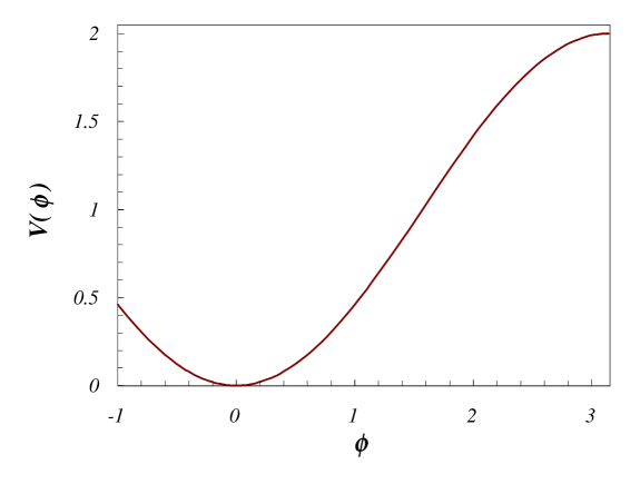
FIG. 1.: The inflationary potential $V=\Delta^{4}(1-\cos\phi)$ (in units of $\Delta^{4}$) Eq. (8), is shown as a function of $\phi$, the angular component of the scalar field $z$.

REFERENCES

- [1] K. Freese, J. Frieman and A.V. Olinto, Phys. Rev. Lett. 65 (1990) 3233. F.C. Adams, J.R. Bond, K. Freese, J.A. Frieman, A.V. Olinto, Phys. Rev. D47 (1993) 426.
- [2] D.H. Lyth and D. Wands, hep-ph/0110002.
- [3] J. Polonyi, Budapest preprint no. KFKI-77-93, 1977
- [4] D. Bailin and A. Love, Supersymmetric Gauge Field Theory and String Theory (Adam Hilger, 1994).
- [5] P.J. Steinhardt, M.S. Turner, Phys. Rev. D29 (1984) 2162.
- [6] For a review and extensive references, see, D.H. Lyth and A. Riotto, Phys. Rep. 314 (1999) 1.
- [7] C.L. Bennett et al (COBE collab.), Astrophys. J. 464 (1996) L1.
- [8] For a review, see, A.R. Liddle and D.H. Lyth, Phys. Rep. 231 (1993) 1.