SPIN-2001/28 ITP-UU-01/35 hep-ph/0111370 November 2001

Inflationary perturbations with multiple scalar fields

Bartjan van Tent

Spinoza Institute/Institute for Theoretical Physics, Utrecht University
P.O.Box 80.195, 3508 TD Utrecht, The Netherlands

and

Stefan Groot Nibbelink

Physikalisches Institut, Universität Bonn
Nußallee 12, D-53115 Bonn, Germany

The calculation of scalar gravitational and matter perturbations during multiple-field inflation valid to first order in slow roll is discussed. These fields may be the coordinates of a non-trivial field manifold and hence have non-minimal kinetic terms. A basis for these perturbations determined by the background dynamics is introduced, and the slow-roll functions are generalized to the multiple-field case. Solutions for a perturbation mode in its three different behavioural regimes are combined, leading to an analytic expression for the correlator of the gravitational potential. Multiple-field effects caused by the coupling to the field perturbation perpendicular to the field velocity can even contribute at leading order. This is illustrated numerically with an example of a quadratic potential. (The material here is based on previous work by the authors presented in hep-ph/0107272.)

PRESENTED AT

COSMO-01
Rovaniemi, Finland,
August 29 – September 4, 2001

1 Introduction

As has been known for a long time, inflation [1, 2] offers a mechanism for the production of density perturbations, which are supposed to be the seeds for the formation of large scale structures in the universe. This mechanism is the magnification of microscopic quantum fluctuations in the scalar fields present during the inflationary epoch into macroscopic matter and metric perturbations. Also, since a part of the primordial spectrum of density perturbations is observed in the cosmic microwave background radiation (CMBR), this mechanism offers one of the most important ways of checking and constraining possible models of inflation, see e.g. [3], especially when combined with large scale structure data [4].

There are two important reasons for considering inflation with multiple scalar fields. The problem of realizing sufficient inflation before a graceful exit from the inflationary era and producing the observed density perturbation spectrum in a model without very unnatural values of the parameters and initial conditions can be solved by the introduction of additional fields. This is the motivation for hybrid inflation models [5, 6]. The other reason is that many theories beyond the standard model of particle physics, like grand unification, supersymmetry or effective supergravity from string theory, contain a lot of scalar fields. Ultimately one would hope to be able to identify those fields that can act as inflatons. In addition such string-inspired supersymmetric models naturally have non-minimal kinetic terms.

The previous two paragraphs outline the motivation for looking at perturbations in multiple-field inflation. A lot of work in this direction has already been done, for example in [7, 8, 9, 6, 10, 11, 12, 13, 14] (more references can be found in [15]). However, most of the previous literature does not consider the most general case, but is usually limited to only two fields and/or minimal kinetic terms. The papers [10, 11] do treat the general case, but the authors do not consider the effect of rotations of the basis, nor do they work out explicitly the particular contribution to the gravitational potential. In [15] we provided a general treatment by computing the scalar gravitational and matter perturbations to first order in slow roll during inflation with multiple real scalar fields that may have non-minimal kinetic terms. Which of these fields acts as inflaton during which part of the inflationary period is determined automatically in our formalism.

This paper basically summarizes part of our previous work [15], concentrating on the calculation of the gravitational potential during inflation, in particular on multiple-field effects like the influence of entropy perturbations during inflation. Necessary background concepts, like the induced field basis and the generalized slow-roll functions, are also discussed. The result is presented in the form of the gravitational correlator at the time of recombination, but for the evolution after inflation only adiabatic perturbations are considered here. This paper also contains a new result for the spectral index $n-1$ of the perturbation spectrum.

2 Background

The gravitational background of the universe is described by the flat Robertson-Walker metric with scale factor $a$:

$$\mathrm{d}s^{2}=-\mathrm{d}t^{2}+a(t)^{2}\mathrm{d}\mathbf{x}^{2}\qquad\Leftrightarrow\qquad\mathrm{d}s^{2}=a(\eta)^{2}\left(-\mathrm{d}\eta^{2}+\mathrm{d}\mathbf{x}^{2}\right).$$ (1)

The comoving time $t$ and conformal time $\eta$ are related by $\mathrm{d}t=a\,\mathrm{d}\eta$. Derivatives with respect to $t$ and $\eta$ are denoted by a dot and a prime, respectively; the associated Hubble parameters are $H\equiv\dot{a}/a$ and ${\cal H}\equiv a^{\prime}/a=aH$. Another useful variable is the number of e-folds $N$, defined by $a(N)=a_{0}\exp(N),$ which can be considered as a time variable as well: $\mathrm{d}N=H\mathrm{d}t={\cal H}\mathrm{d}\eta.$

For the matter content of the universe we assume an arbitrary number of real scalar fields, which are the components of a vector ${\boldsymbol{\phi}}$. Apart from a generic potential $V({\boldsymbol{\phi}})$ we allow for the possibility of non-minimal kinetic terms, encoded by a field metric $\mathbf{G}$. In other words, the scalar fields may be the coordinates of a real field manifold with a non-trivial metric $\mathbf{G}$. This is a common situation in for example supergravity models, where the (complex) scalar fields parameterize a so-called Kähler manifold with a metric that is the second mixed derivative of the Kähler potential. Since a complex field can always be written in terms of two real fields, our treatment with real scalars is sufficiently general to be easily applicable to these special manifolds.

The Einstein and field equations lead to the following equations of motion for the homogeneous background:

$$H^{2}=\frac{\kappa^{2}}{3}\left(\frac{1}{2}|\dot{{\boldsymbol{\phi}}}|^{2}+V\right),\qquad\dot{H}=-\frac{1}{2}\kappa^{2}|\dot{{\boldsymbol{\phi}}}|^{2},\qquad{\cal D}_{t}\dot{{\boldsymbol{\phi}}}+3H\dot{{\boldsymbol{\phi}}}+\mathbf{G}^{-1}\boldsymbol{\nabla}^{T}V=0.$$ (2)

Here we have defined the covariant time derivative on a vector in field space as ${\cal D}_{t}A^{a}=\dot{A}^{a}+\Gamma^{a}_{bc}\dot{\phi}^{b}A^{c}.$ (Indices $a,b,\ldots$ are used for components in field space and $\Gamma^{a}_{bc}$ is the connection associated with the field metric $\mathbf{G}$.) The $\boldsymbol{\nabla}$ is used for covariant derivatives with respect to the fields: $(\boldsymbol{\nabla}V)_{a}=\partial V/\partial\phi^{a}$. The length of a vector is given by $|\mathbf{A}|=\sqrt{\mathbf{A}\cdot\mathbf{A}}$, with the inner product defined by $\mathbf{A}\cdot\mathbf{B}=\mathbf{A}^{\dagger}\mathbf{B}=\mathbf{A}^{T}\mathbf{G}\mathbf{B}$. The quantity $\kappa$ is the inverse reduced Planck mass: $\kappa^{2}\equiv 8\pi G=8\pi/M_{P}^{2}$.

The background field dynamics induce a prefered basis on the field manifold. The first unit vector $\mathbf{e}_{1}$ is given by the direction of the field velocity $\dot{{\boldsymbol{\phi}}}$. The second unit vector $\mathbf{e}_{2}$ points in the direction of that part of the field acceleration ${\cal D}_{t}\dot{{\boldsymbol{\phi}}}$ that is perpendicular to the first unit vector $\mathbf{e}_{1}$. Hence:

$$\mathbf{e}_{1}=\frac{\dot{{\boldsymbol{\phi}}}}{|\dot{{\boldsymbol{\phi}}}|},\qquad\mathbf{e}_{2}=\frac{\mathbf{P}^{\perp}{\cal D}_{t}\dot{{\boldsymbol{\phi}}}}{|\mathbf{P}^{\perp}{\cal D}_{t}\dot{{\boldsymbol{\phi}}}|},\qquad\qquad\mathbf{P}^{\perp}=\mathbf{1}-\mathbf{P}^{\parallel}=\mathbf{1}-\mathbf{e}_{1}^{\;}\mathbf{e}_{1}^{\dagger},$$ (3)

with $\mathbf{P}^{\parallel}$ the projection on the direction $\dot{{\boldsymbol{\phi}}}$. This Gram-Schmidt orthogonalization procedure can be continued to construct the remaining basis vectors [15], but the first two are the only ones we need here.

We can now define the following multiple-field slow-roll functions:

$${\tilde{\epsilon}}=-\frac{\dot{H}}{H^{2}},\qquad\qquad\tilde{\boldsymbol{\eta}}=\frac{{\cal D}_{t}\dot{{\boldsymbol{\phi}}}}{H|\dot{{\boldsymbol{\phi}}}|},\qquad\qquad\tilde{\boldsymbol{\xi}}=\frac{{\cal D}_{t}^{2}\dot{{\boldsymbol{\phi}}}}{H^{2}|\dot{{\boldsymbol{\phi}}}|},$$ (4)

of which we can take components with respect to the basis defined above, for example ${\tilde{\eta}}^{\parallel}=\mathbf{e}_{1}\cdot\tilde{\boldsymbol{\eta}}$, ${\tilde{\eta}}^{\perp}=\mathbf{e}_{2}\cdot\tilde{\boldsymbol{\eta}}$ and ${\tilde{\xi}}^{\parallel}=\mathbf{e}_{1}\cdot\tilde{{\boldsymbol{\xi}}}$. Again, one can easily define slow-roll functions of higher order [15]. With these definitions as short-hand notation we can rewrite the background equations of motion in the following form, which is still exact:

$$H =\frac{\kappa}{\sqrt{3}}\sqrt{V}\left(1-\frac{1}{3}{\tilde{\epsilon}}\right)^{-1/2},$$ (5)

$$\dot{{\boldsymbol{\phi}}}+\frac{1}{\kappa\sqrt{3}}\frac{1}{\sqrt{V}}\,\mathbf{G}^{-1}\boldsymbol{\nabla}^{T}V =-\sqrt{\frac{2}{3}}\sqrt{V}\frac{\sqrt{{\tilde{\epsilon}}}}{1-\frac{1}{3}{\tilde{\epsilon}}}\left(\frac{1}{3}\tilde{\boldsymbol{\eta}}+\frac{\frac{1}{3}{\tilde{\epsilon}}\,\mathbf{e}_{1}}{1+\sqrt{1-\frac{1}{3}{\tilde{\epsilon}}}}\right).$$ (6)

The assumption that the slow-roll functions ${\tilde{\epsilon}}$ and $\tilde{{\boldsymbol{\eta}}}$ are (much) smaller than unity is called the slow-roll approximation. (The second order slow-roll function $\tilde{{\boldsymbol{\xi}}}$ is assumed to be of an order comparable to ${\tilde{\epsilon}}^{2}$, ${\tilde{\epsilon}}{\tilde{\eta}}^{\parallel}$, etc.) If this assumption is valid, we can use expansions in powers of these slow-roll functions to estimate the relevance of various terms in a given expression. For example, to first order the Friedmann equation (5) is approximated by replacing $(1-{\tilde{\epsilon}}/3)^{-1/2}$ by $(1+{\tilde{\epsilon}}/6)$. The background field equation up to and including first order is given by (6) with the right-hand side set to zero, as all those terms are order $3/2$ or higher.

3 Perturbations

On top of the homogeneous background treated in the previous section there are small quantum fluctuations. We consider only scalar perturbations and write the matter and metric perturbations as follows [16]

$${\boldsymbol{\phi}}^{\mathrm{full}}(\eta,\mathbf{x})={\boldsymbol{\phi}}(\eta)+{\boldsymbol{\delta}}{\boldsymbol{\phi}}(\eta,\mathbf{x}),$$

$$g_{\mu\nu}^{\mathrm{full}}(\eta,\mathbf{x})=g_{\mu\nu}(\eta)+\delta g_{\mu\nu}(\eta,\mathbf{x})=a^{2}(\eta)\left(\hskip-5.0pt\begin{array}[]{cccccccccc}-1&0\\ 0&\delta_{ij}\end{array}\hskip-5.0pt\right)-2a^{2}(\eta)\Phi(\eta,\mathbf{x})\left(\hskip-5.0pt\begin{array}[]{cccccccccc}1&0\\ 0&\delta_{ij}\end{array}\hskip-5.0pt\right).$$ (11)

All equations are linearized with respect to the perturbation quantities. The gravitational potential $\Phi(\eta,\mathbf{x})$ describes the scalar metric perturbations and is a quantity we are interested in, as it is related to the temperature fluctuations in the cosmic microwave background radiation by means of the Sachs-Wolfe effect.

Instead of using ${\boldsymbol{\delta}}{\boldsymbol{\phi}}$ and $\Phi$ to describe the perturbations, it turns out to be more convenient to use the so-called generalized Mukhanov-Sasaki variables $\mathbf{q}$ and $u$, as well as a short-hand notation $\theta$, defined by

$$u=\frac{\Phi}{\kappa\sqrt{2}\,H\sqrt{{\tilde{\epsilon}}}},\qquad\qquad\mathbf{q}=a\left({\boldsymbol{\delta}}{\boldsymbol{\phi}}+\frac{\Phi}{{\cal H}}\,{\boldsymbol{\phi}}^{\prime}\right),\qquad\qquad\theta=\frac{\kappa}{\sqrt{2}}\frac{1}{a\sqrt{{\tilde{\epsilon}}}}.$$ (12)

These redefinitions remove first order time derivatives, so that it is easier to understand the behaviour of the solutions, and are necessary for quantization. The perturbation equations in terms of spatial Fourier modes $\mathbf{k}$ now read [15]

$$u_{\mathbf{k}}^{\prime\prime}+\left(k^{2}-\frac{\theta^{\prime\prime}}{\theta}\right)u_{\mathbf{k}}={\cal H}{\tilde{\eta}}^{\perp}\mathbf{e}_{2}\cdot\mathbf{q}_{\mathbf{k}},\qquad\qquad{\cal D}_{\eta}^{2}\mathbf{q}_{\mathbf{k}}+(k^{2}+{\cal H}^{2}{{\boldsymbol{\Omega}}})\mathbf{q}_{\mathbf{k}}=0,$$

$${{\boldsymbol{\Omega}}}\equiv\frac{1}{H^{2}}\tilde{\mathbf{M}}^{2}-(2-{\tilde{\epsilon}})\mbox{\small 1}\mbox{1}-2{\tilde{\epsilon}}\Bigl{(}(3+{\tilde{\epsilon}})\mathbf{P}^{\parallel}+\mathbf{e}_{1}^{\;}\tilde{{\boldsymbol{\eta}}}^{\dagger}+\tilde{{\boldsymbol{\eta}}}\mathbf{e}_{1}^{\dagger}\Bigr{)}.$$ (13)

Here the effective mass matrix $\tilde{\mathbf{M}}^{2}$ is defined by $\tilde{\mathbf{M}}^{2}\equiv\mathbf{G}^{-1}\boldsymbol{\nabla}^{T}\boldsymbol{\nabla}V-\mathbf{R}(\dot{{\boldsymbol{\phi}}},\dot{{\boldsymbol{\phi}}}),$ with $\mathbf{R}$ the curvature tensor on the field manifold, $[\mathbf{R}(\mathbf{B},\mathbf{C})\mathbf{D}]^{a}=R^{a}_{\;bcd}B^{b}C^{c}D^{d}$. From its definition we can derive that $\theta^{\prime\prime}/\theta$ is exactly given by $\theta^{\prime\prime}/\theta={\cal H}^{2}(2{\tilde{\epsilon}}+{\tilde{\eta}}^{\parallel}+2({\tilde{\eta}}^{\parallel})^{2}-({\tilde{\eta}}^{\perp})^{2}-{\tilde{\xi}}^{\parallel}).$ We see that in the multiple-field case the redefined gravitational potential $u$ is coupled to the field perturbation in the $\mathbf{e}_{2}$ direction. In the literature (see e.g. [9]) perturbations in the $\mathbf{e}_{1}$ direction are called adiabatic perturbations, while perturbations in the other directions are called entropy perturbations. This coupling of the gravitational potential to the entropy perturbations is suppressed by the slow-roll function ${\tilde{\eta}}^{\perp}$, so one could a priori expect the contribution of this inhomogeneous term to be only important at first order. However, because of integration interval effects it turns out that it can contribute even at leading order, as shown in the example in section 4.

To quantize the perturbations, we explicitly choose to work in the basis $\{\mathbf{e}_{1},\mathbf{e}_{2},\ldots\}$ defined in the previous section, denoting vectors in that basis with non-bold symbols: $q^{T}=(q_{n})=(\mathbf{e}_{n}\cdot\mathbf{q})$. Although this has several advantages, most importantly it results in a standard canonical normalization of $\frac{1}{2}(q^{\prime})^{T}q^{\prime}$ in the Lagrangean, independent of the field metric $\mathbf{G}$, making quantization straightforward. Of course there is the price that terms with $Z$ (see below) appear, but these can be dealt with. We can write $\hat{q}(\eta)=Q(\eta)\hat{a}^{\dagger}+Q^{*}(\eta)\hat{a},$ with constant creation and annihilation operator vectors $\hat{a}^{\dagger}$ and $\hat{a}$ and a matrix function $Q(\eta)$ that satisfies the classical equation of motion. Finally we perform a rotation $Q=R{\tilde{Q}}$ to simplify this equation of motion and find:

$${\tilde{Q}}^{\prime\prime}+(k^{2}+{\cal H}^{2}\tilde{\Omega}){\tilde{Q}}=0,\qquad R^{\prime}+{\cal H}ZR=0,\qquad Z_{mn}=\frac{1}{{\cal H}}\,\mathbf{e}_{m}\cdot{\cal D}_{\eta}\mathbf{e}_{n},$$ (14)

with $\tilde{\Omega}=R^{-1}\Omega R$. The matrix $Z$ is anti-symmetric, first order in slow roll and only non-zero for $m=n\pm 1$. The presence of this matrix is caused by the fact that the basis vectors are in general not static in field space because of the background dynamics. Working out the definitions, one can easily show that $Z_{21}={\tilde{\eta}}^{\perp}$; general expressions are given in [15].

Considering the equations (13) and (14) for $u$ and ${\tilde{Q}}$ and realizing that ${\cal H}$ grows rapidly during inflation, while $k$ is a constant per mode, we see that their solutions change dramatically around the time $\eta_{\cal H}$ when a scale crosses the Hubble scale (‘passes through the horizon’), defined by ${\cal H}(\eta_{\cal H})=k$. Hence there are three regions of interest: sub-horizon (${\cal H}\ll k$), transition (${\cal H}\sim k$) and super-horizon (${\cal H}\mg k$). (Notice that we are considering a single, though arbitrary, mode $\mathbf{k}$ here, on which the resulting expressions will depend.) The equations in the sub-horizon region are easily solved, but the oscillatory solutions there are irrelevant for the correlators we are interested in.

In the transition region we can only solve the equations analytically if we make the additional assumption that the slow-roll functions are constant. Since the derivatives of the slow-roll functions are one order higher in slow roll, this is a consistent approximation to first order, provided that the transition region is small enough. The solution for $Q$ valid to first order in slow roll in the neighbourhood of $\eta_{\cal H}$, taking into account the correct initial conditions, can be written in terms of a Hankel function:

$$Q(\eta)=\sqrt{\frac{\pi\eta}{4}}\,H_{\nu_{\cal H}}^{(1)}(k\eta),\qquad\nu_{\cal H}=\frac{3}{2}\mbox{\small 1}\mbox{1}+\delta_{\cal H},\qquad\delta_{\cal H}={\tilde{\epsilon}}_{\cal H}\mbox{\small 1}\mbox{1}-\frac{\tilde{M}_{\cal H}^{2}}{3H_{\cal H}^{2}}+2{\tilde{\epsilon}}_{\cal H}\,e_{1}^{\;}e_{1}^{T}.$$ (15)

Here the additional assumption has been made that also those components of the matrix $\tilde{M}_{\cal H}^{2}/H_{\cal H}^{2}$ that cannot be expressed in terms of the slow-roll functions defined in (4), are nonetheless of first order in slow roll. In particular this puts constraints on the curvature tensor of the field manifold. The matrix $Z$ appearing in equation (14) for $R$ is a possible source of multiple-field effects. However, it turns out that in generic situations the effects of the rotation of the basis during the transition region encoded by $Z$ are beyond first order so that it does not appear in the first order result (15), although it might be important if ${\tilde{\eta}}^{\perp}$ peaks around $\eta_{\cal H}$.

Solutions for $u$ and $Q$ can also be determined analytically to first order in the super-horizon region. However, matching the solutions in the super-horizon region to those in the transition region to determine the constants of integration is not trivial, as there is no region of overlap where both solutions are valid to first order. Hence the standard method of continuously differentiable matching at a certain time scale cannot be applied. In particular one should not simply match at $\eta_{\cal H}$, as the assumption of neglecting $k$, that is necessary to obtain the analytic super-horizon solution, is not valid there.

We solved this problem in [15] by setting up series expansions in $k\eta$ for both the super-horizon and transition solutions. We found that the leading order powers in these asymptotic expansions can exactly be identified to first order, for both the decaying and non-decaying independent solutions, which can already at zeroth order be distinguished from each other. Since the transition and super-horizon solutions are approximations of the complete solution of the same equation of motion, the coefficients in front of the series have to be equal as well. In this way the solution in the super-horizon region is determined completely to first order.

The final result for $u$ at later times in the super-horizon region (i.e. neglecting terms that are suppressed by the scale factor) to first order in slow roll is [15]:

$$u_{\mathbf{k}}(\eta)=u_{P\,\mathbf{k}}^{\;}+D_{\mathbf{k}}\theta\int_{\eta_{\cal H}}^{\eta}\frac{\mathrm{d}\eta^{\prime}}{\theta^{2}},\qquad u_{P\,\mathbf{k}}=\theta\int^{\eta}_{\eta_{\cal H}}\frac{\mathrm{d}\eta^{\prime}}{\theta^{2}}\int^{\eta^{\prime}}_{\eta_{\cal H}}\mathrm{d}\eta^{\prime\prime}\,{\cal H}\theta{\tilde{\eta}}^{\perp}q_{2\,\mathbf{k}},$$ (16)

with $D_{\mathbf{k}}=-\frac{1}{2}\frac{e^{-i\pi\delta_{\cal H}}}{i\sqrt{2k}}\,\theta_{\cal H}e_{1}^{T}\left((1-{\tilde{\epsilon}}_{\cal H})\mbox{\small 1}\mbox{1}+B\delta_{\cal H}\right)\hat{a}^{\dagger}+\mbox{c.c.}$ and $u_{P}$ the particular solution caused by the inhomogeneous source term in the equation of motion (13) for $u$ and $B\equiv 2-\gamma_{E}-\ln 2\approx 0.7297$. Switching back to the real gravitational potential $\Phi$ we have the complete solution at the end of inflation, so including the effect of the perpendicular field or entropy perturbations during inflation. Considering here for simplicity only adiabatic perturbations after inflation we can compute the vacuum correlator of the gravitational potential at the time of recombination when the CMBR was formed [15]:

$$|\delta_{\mathbf{k}}|^{2}\equiv\frac{k^{3}}{2\pi^{2}}\langle\Phi_{\mathbf{k}}^{2}\rangle_{t_{rec}}=\frac{9}{25}\,\frac{\kappa^{2}}{8\pi^{2}}\frac{H_{\cal H}^{2}}{{\tilde{\epsilon}}_{\cal H}}\Bigl{[} (1-2{\tilde{\epsilon}}_{\cal H})(1+U_{P\,e}^{T}U_{P\,e})$$

$$+2B\left((2{\tilde{\epsilon}}_{\cal H}+{\tilde{\eta}}^{\parallel}_{\cal H})+2{\tilde{\eta}}^{\perp}_{\cal H}e_{2}^{T}U_{P\,e}+U_{P\,e}^{T}\delta_{\cal H}U_{P\,e}\right)\Bigr{]}.$$ (17)

Here $U_{P\,e}=U_{P}(\eta_{e})$, with $\eta_{e}$ the end time of inflation, is defined by

$$U_{P}^{T}=2\sqrt{{\tilde{\epsilon}}_{\cal H}}\int_{\eta_{\cal H}}^{\eta}\mathrm{d}\eta^{\prime}\,{\cal H}\frac{{\tilde{\eta}}^{\perp}}{\sqrt{{\tilde{\epsilon}}}}\,\frac{a_{\cal H}}{a}\,e_{2}^{T}QQ_{\cal H}^{-1}$$ (18)

and we have used the fact that $U_{P}$ has no component in the $e_{1}$ direction. More information on $U_{P}$, in particular on how to rewrite it in terms of background quantities only, can be found in [15]. Apart from this amplitude we can also compute the slope of the spectrum. This spectral index can be determined one order further, but most important is its leading (first) order part:

$$n-1\equiv\frac{\partial\ln|\delta_{k}|^{2}}{\partial\ln k}=-4{\tilde{\epsilon}}_{\cal H}-2{\tilde{\eta}}^{\parallel}_{\cal H}+\frac{2U_{P\,e}^{T}(2{\tilde{\epsilon}}_{\cal H}+{\tilde{\eta}}^{\parallel}_{\cal H}-\delta_{\cal H})U_{P\,e}-4{\tilde{\eta}}^{\perp}_{\cal H}e_{2}^{T}U_{P\,e}}{1+U_{P\,e}^{T}U_{P\,e}}.$$ (19)

The explicit multiple field terms in the results for $|\delta_{\mathbf{k}}|^{2}$ and $n-1$ are the contributions of the terms with $U_{P\,e}$ and ${\tilde{\eta}}^{\perp}_{\cal H}$, which are absent in the single-field case. Since they are both to a large extent determined by ${\tilde{\eta}}^{\perp}$, we see that the behaviour of ${\tilde{\eta}}^{\perp}$ during the last 60 e-folds of inflation is crucial to determine whether multiple-field effects are important.

4 Example

In this section the example of a quadratic potential on a flat field manifold is briefly discussed to illustrate the theory. In this case it is possible to compute $U_{P\,e}$ explicitly and we show that it can indeed contribute already at zeroth order to the gravitational correlator, despite the slow-roll factor ${\tilde{\eta}}^{\perp}$.

The potential is $V=\frac{1}{2}\kappa^{-2}\,{\boldsymbol{\phi}}^{T}\mbox{{m}}^{2}{\boldsymbol{\phi}}$ with $\mbox{{m}}^{2}$ a general symmetric mass matrix given in units of the Planck mass $\kappa^{-1}$. With a trivial field metric and initial condition ${\boldsymbol{\phi}}(0)={\boldsymbol{\phi}}_{0}$ we can write the general first order slow-roll solution for ${\boldsymbol{\phi}}$ in terms of a single scalar function $\psi(t)$. Even without knowing this function explicitly we can determine $U_{P\,e}$ [15]:

$${\boldsymbol{\phi}}(t)=e^{-\frac{1}{2}\mathbf{m}^{2}\psi(t)}{\boldsymbol{\phi}}_{0},\qquad\qquad U_{P\,e}^{T}=-\frac{\kappa\sqrt{{\tilde{\epsilon}}_{\cal H}}}{\sqrt{2}}\,\phi_{\cal H}^{T}P_{1}^{\perp}.$$ (20)

This expression for $U_{P\,e}$ assumes slow roll, but is valid at the end of inflation provided that ${\tilde{\eta}}^{\perp}$ goes to zero.

For the case of two fields with masses $m_{1}=1\cdot 10^{-5}$ and $m_{2}=2.5\cdot 10^{-5}$ and initial conditions $\phi_{1}=20$ and $\phi_{2}=25$ in Planck units, the results for the slow-roll functions and $U_{P}$ as a function of the number of e-folds $N$ are plotted in figure 1. We see that in this case ${\tilde{\eta}}^{\perp}$ indeed goes to zero at the end of inflation after reaching a maximum during the last 60 e-folds, and $U_{P}$ reaches a constant value long before a possible break-down of slow roll. Values for the gravitational correlator amplitude $|\delta_{\mathbf{k}}|^{2}$ and spectral index $n-1$ are given in table 1.

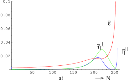
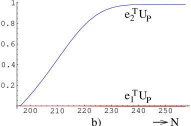
Figure 1: a) The slow-roll functions and b) the particular contribution $U_{P}$ to the gravitational correlator as a function of the number of e-folds $N$ in the model with two fields on a flat manifold with a quadratic potential with masses $m_{1}=1\cdot 10^{-5}$, $m_{2}=2.5\cdot 10^{-5}$ and initial conditions $\phi_{1}=20$, $\phi_{2}=25$.

	$|\delta_{\mathbf{k}}|^{2}$	Contribution	Error	$n-1$	Contribution
Homogeneous	$1.55\cdot 10^{-9}$	0.505	0.0001	$-0.0377$	0.584
Particular	$1.52\cdot 10^{-9}$	0.495	0.0006	$-0.0269$	0.416
Total	$3.08\cdot 10^{-9}$	1	0.0003	$-0.0646$	1

Table 1: The amplitude $|\delta_{\mathbf{k}}|^{2}$ and slope $n-1$ of the vacuum correlator of the gravitational potential are separated into a purely homogeneous and a (mixed) particular part. Given are their values and their relative contributions to the total according to our analytical slow-roll results (17) and (19) combined with (20). For the amplitude we also calculated exact numerical results and give here the relative error between those and our analyical approximations.

The results for the amplitude and the slope are split into a homogeneous part (all terms without $U_{P\,e}$) and a particular part (the rest, including mixing terms). Everything is evaluated for the mode $k$ that crosses the horizon 60 e-folds before the end of inflation. From the column giving the relative errors between our first order analytical results (17) and (20) on the one hand, and the exact numerical result on the other, we see that these results agree with our claim that we computed the correlator to first order in slow roll: the relative errors are (much) smaller than ${\cal O}({\tilde{\epsilon}}_{\cal H})$. We also see that our slow-roll approximation for $U_{P}$ is indeed still very good at the end of inflation, as indicated by the small error in the particular part. From the other columns we see that the particular solution terms are responsible for almost half the total result in this model, both for the amplitude and the spectral index. Hence neglecting these terms to leading order, which might naively be done because they couple with a ${\tilde{\eta}}^{\perp}$ in (13), can be dangerous.

5 Conclusions

In this paper we have given a summary of our general treatment [15] for scalar perturbations on a flat Robertson-Walker spacetime in the presence of an arbitrary number of scalar fields that take values on a curved field manifold during slow-roll inflation. These are the kind of systems that one typically obtains from (string-inspired) high-energy models. Here we concentrated on the calculation of the vacuum correlator of the gravitational potential to first order in slow roll, which is related to the temperature fluctuations that are observed in the CMBR.

A discussion of the background served as the foundation for this analysis. The background field dynamics naturally induce an orthonormal basis $\{\mathbf{e}_{1},\mathbf{e}_{2},\ldots\}$ on the tangent bundle of the field manifold. This makes a separation between effectively single-field and truly multiple-field contributions possible and is a necessary ingredient for correct quantization of the perturbations. We also modified the definitions of the well-known slow-roll parameters to define slow-roll functions in terms of derivatives of the Hubble parameter and the background field velocity for the case of multiple scalar field inflation. These slow-roll functions are vectors, which can be decomposed in the basis induced by the field dynamics. For example, the slow-roll function ${\tilde{\eta}}^{\perp}$ measures the size of the field acceleration perpendicular to the field velocity. Because we did not make the assumption that slow roll is valid in the definition of the slow-roll functions, it is often possible to identify these slow-roll functions in exact equations of motion and make decisions about neglecting some of the terms.

We generalized the combined system of gravitational and matter perturbations of Mukhanov et al. [16] by defining the Mukhanov-Sasaki variables as a vector on the scalar field manifold. The gravitational potential only couples to the scalar field perturbation in the direction $\mathbf{e}_{2}$ with a slow-roll factor ${\tilde{\eta}}^{\perp}$. First order solutions were found in the three different regimes that reflect the change of behaviour for a given mode when it crosses the Hubble scale. Using a procedure of analytically identifying leading order terms in asymptotic expansions in $k\eta$ we were able to relate the solutions in the different regions and find the complete first order result for the gravitational potential at the end of inflation. Considering only adiabatic perturbations after inflation we could give this result in terms of the vacuum correlator of the gravitational potential at the time of recombination. We also determined the spectral index $n-1$.

Multiple-field effects are important in the adiabatic perturbations at the time of recombination if ${\tilde{\eta}}^{\perp}$ is sizable during the last 60 e-folds of inflation. The most important source of multiple-field effects is the particular solution of the gravitational potential caused by the perpendicular field perturbations during inflation. We found in our numerical example of multiple scalar fields on a flat manifold with a quadratic potential that this term can contribute already at leading order, even though it enters with a slow-roll factor in the equation of motion. This is true for both the amplitude and the slope of the spectrum.

ACKNOWLEDGEMENTS

This work is supported by the European Commission RTN programme HPRN-CT-2000-00131. S.G.N. is also supported by piority grant 1096 of the Deutsche Forschungsgemeinschaft and European Commission RTN programme HPRN-CT-2000-00148/00152.

References

- [1] A. H. Guth, Phys. Rev. D 23 (1981) 347.
- [2] A. D. Linde, Chur, Switzerland: Harwood (1990) 362 p. (Contemporary concepts in physics, 5).
- [3] W. H. Kinney, A. Melchiorri and A. Riotto, Phys. Rev. D 63 (2001) 023505 [arXiv:astro-ph/0007375].
- [4] S. Hannestad, S. H. Hansen, F. L. Villante and A. J. Hamilton, arXiv:astro-ph/0103047.
- [5] A. D. Linde, Phys. Rev. D 49 (1994) 748 [arXiv:astro-ph/9307002].
- [6] D. H. Lyth and A. Riotto, Phys. Rept. 314 (1999) 1 [arXiv:hep-ph/9807278].
- [7] D. Polarski and A. A. Starobinsky, Nucl. Phys. B 385 (1992) 623.
- [8] J. Garcia-Bellido and D. Wands, Phys. Rev. D 53 (1996) 5437 [arXiv:astro-ph/9511029].
- [9] C. Gordon, D. Wands, B. A. Bassett and R. Maartens, Phys. Rev. D 63 (2001) 023506 [arXiv:astro-ph/0009131].
- [10] M. Sasaki and E. D. Stewart, Prog. Theor. Phys. 95 (1996) 71 [arXiv:astro-ph/9507001].
- [11] T. T. Nakamura and E. D. Stewart, Phys. Lett. B 381 (1996) 413 [arXiv:astro-ph/9604103].
- [12] D. Polarski and A. A. Starobinsky, Phys. Rev. D 50 (1994) 6123 [arXiv:astro-ph/9404061].
- [13] D. Langlois, arXiv:astro-ph/9906080.
- [14] J. c. Hwang and H. Noh, arXiv:astro-ph/0103244.
- [15] S. Groot Nibbelink and B. J. van Tent, arXiv:hep-ph/0107272.
- [16] V. F. Mukhanov, H. A. Feldman and R. H. Brandenberger, Phys. Rept. 215 (1992) 203.