TESIS DOCTORAL

Phenomenology of Bilinear Broken

R–parity

Departament de Física Teòrica

Diego Alejandro Restrepo Quintero

Abstract

The straightforward supersymmetrization of the Standard Model (SM) results in a phenomenologically inconsistent theory in which Baryon number ($B$) and Lepton number ($L$) are violated by dimension 4 operators, inducing fast proton decay. Proton stability allows only for separate $L$ or $B$ violation and, if neutrinos are massive Majorana particles, $L$ violating terms must be present. In this thesis I will study a Supersymmetric Standard Model (SSM) realization with $B$ conservation and minimal $L$ violation. In this framework $L$ is mildly violated only by super–renormalizable terms, allowing for small neutrino Majorana masses. This model is more predictive than the Baryon–Parity SSM. The induced dimension 4 $L$ violating couplings are not arbitrary, and automatically satisfy all experimental constraints. After introducing the theoretical framework for supersymmetric models without Lepton number, I will discuss the phenomenology of the (unstable) lightest neutralino and of the lightest stop. I will show that the leptonic decays of the stop can be related to the neutrino parameters, and in particular their measurement can indirectly probe the size of the solar neutrinos mixing angle.

Resumen

El Modelo Estándar Supersimétrico (MES) es el modelo supersimétrico con mínimo número de partículas correspondientes a aquellas del Modelo Estándar (ME), un doblete de Higgs adicional y todos los compañeros supersimétricos de las partículas del ME. El MES permite la aparición simultanea de términos que violan número leptónico y bariónico y de este modo es excluido debido a que el protón decae a través de interacciones electrodébiles. Sin embargo es bien conocido que la estabilidad del protón permite la presencia ya sea de violación de número leptónico o de la violación de número bariónico. De hecho, si los neutrinos tienen masa como es sugerido por las anomalías solar y atmosférica no existe una razón de peso para asumir que los términos que violan número leptónico estén ausentes. En este trabajo estudiaremos la realización del MES con conservación de número bariónico y violación mínima de número leptónico. Los únicos términos con violación de número leptónico en este caso provienen del término de masa más general que permite la invarianza gauge en el superpotencial del MES. Al modelo correspondiente le llamaremos Modelo Estándar Supersimétrico Superrenormalizable (MESS). El MESS es más predictivo y teóricamente más atractivo que el MES con conservación de número bariónico pero con términos arbitrarios de violación de número leptónico y en general satisface todos las restricciones que surgen de esta violación.

En el MESS la Partícula Supersimétrica más Liviana (PSL) puede decaer. En particular estudiaremos la fenomenología esperada del neutralino en LEP2. En el caso de partículas supersimétricas con mayor masa que la PSL, los decaimientos que violan número leptónico pueden llegar a ser detectables en los aceleradores, incluso en el caso de masas de neutrinos tan pequeñas como las sugeridas por las anomalías de neutrinos. Especialmente interesante en este caso son los decaimientos que violan número leptónico del stop (compañero supersimétrico del quark top), y que serán estudiados en este trabajo. Estos decaimientos implican la posibilidad de probar el ángulo de mezcla solar y así la posibilidad de relacionar la física de colisionadores de alta energía con los experimentos sobre oscilación de neutrinos solares.

Contents

1. Introduction
2. 1 One generation Supersymmetric Standard Model
   1. 1.1 Supersymmetric Lagrangian
   2. 1.2 One generation Supersymmetric Standard Model
      1. 1.2.1 One generation SSM lagrangian
      2. 1.2.2 Basis independent parameters
      3. 1.2.3 Origin of Neutrino Masses
3. 2 Supersymmetric Standard Models
   1. 2.1 Possible $X$ symmetries
   2. 2.2 Gauge Discrete symmetries
      1. 2.2.1 Superrenormalizable Supersymmetric Standard Model (Bilinear Model)
   3. 2.3 Alternative SSSM origin
      1. 2.3.1 Flavor symmetries
   4. 2.4 Phenomenology of SSSM
4. 3 The mass spectrum of the SSSM
   1. 3.1 Chargino mass matrix
   2. 3.2 Neutralino mass matrix
   3. 3.3 The squark mass spectrum
   4. 3.4 Scalar Mass Matrices
      1. 3.4.1 Charged scalars
      2. 3.4.2 CP–Even Neutral Scalars
      3. 3.4.3 CP–Odd Neutral Scalars
5. 4 Sparticle decays
   1. 4.1 Decays of neutralinos
   2. 4.2 Squark decays
      1. 4.2.1 Two body decays
      2. 4.2.2 Three body decays
6. 5 Numerical Results
   1. 5.1 Sugra Case
      1. 5.1.1 Neutralinos
      2. 5.1.2 Lightest Stop Two-Body Decays in SUGRA
      3. 5.1.3 Two-Body Decays of the Lightest Stop: the SSSM case
   2. 5.2 Three Body Decays of stop
7. 6 Conclusions
8. A Constraints on horizontal charges
9. B Complete formulas for 2 body decays
   1. B.1 An explicit calculation
   2. B.2 Couplings Neutralino–Squark-Quark
   3. B.3 Couplings Chargino-Squark-Quark
10. Bibliography
11. Index
12. Agradecimientos

List of Figures

1. 2.1 Possible contribution to proton decay, involving $\kappa^{\prime}_{ijkl}$
2. 2.2 Possibilities of $R_{p}$ breaking
3. 2.3 Tree-level neutrino mass dependence
4. 4.1 Feynman graphs for the decay $\tilde{\chi}^{0}_{1}\to\nu_{3}\,f\,\bar{f}$ where $f\neq\tau$.
5. 5.1 Neutralino cross section
6. 5.2 Contour lines of the neutralino production cross sections
7. 5.3 Decay length of the lightest neutralino in cm
8. 5.4 Decay length of the lightest neutralino in cm
9. 5.5 Branching ratios for $\tilde{\chi}^{0}_{1}\to 3\,\nu$
10. 5.6 Branching ratios for $\tilde{\chi}^{0}_{1}\to\nu_{3}\,l^{+}\,l^{-}$
11. 5.7 Branching ratios for $\tilde{\chi}^{0}_{1}\to\nu_{3}\,q\,\bar{q}$
12. 5.8 Branching ratios for $\tilde{\chi}^{0}_{1}\to\nu_{l}\,\tau^{\pm}\,l^{\mp}$
13. 5.9 Branching ratios for $\tilde{\chi}^{0}_{1}\to\tau^{\pm}\,q\,\bar{q}^{\prime}$
14. 5.10 Branching ratios for $\tilde{\chi}^{0}_{1}\to\nu_{3}\,b\,\bar{b}$
15. 5.11 Branching ratios for $\tilde{\chi}^{0}_{1}\to\nu_{3}\,\tau^{+}\,\tau^{-}$
16. 5.12 Branching ratios for $\tilde{\chi}^{0}_{1}\to\nu_{3}\,\gamma$
17. 5.13 Kinematical regions in the $m_{{\tilde{t}}_{1}}$–$m_{{\tilde{\chi}}_{1}^{+}}$ plane
18. 5.14 Comparison between the exact numerical calculation and the one–step approximation for the $\tilde{t}_{1}\to c\,\tilde{\chi}_{1}^{0}$ decay width.
19. Region I
20. 5.17 Contours of $BR({\tilde{t}}_{1}\to b\,\tau)>BR({\tilde{t}}_{1}\to b\tilde{\chi}_{1}^{+})$
21. Region II
22. 5.20 Universality condition $B_{0}=B_{3}$ at the unification scale as a function of $A_{0}$.
23. Effects of non–Universality
24. 5.23 Minimum value of the $\nu_{3}$ mass as a function of $\sin\xi$
25. 5.24 Branching ratios for the $\tilde{t}_{1}$ as a function of $\cos\theta_{\tilde{t}}$
26. 5.25 Branching ratios for ${\tilde{t}}_{1}$ decays
27. 5.26 Ratio of branching ratios: $BR({\tilde{t}}_{1}\to be^{+})/BR({\tilde{t}}_{1}\to b\mu^{+})$ as a function of $(\mu_{1}/\mu_{2})^{2}$

List of Tables

1. 1.1 Estimated magnitude of $L$ violating parameters.
2. 2.1 Possible models arising for discrete symmetries
3. 2.2 Possibilities of low energy $L$ or $B$ violating superpotential renormalizable terms
4. 2.3 Models of horizontal charge differences
5. 2.4 Final charge differences
6. 4.1 Contributions involved in the lightest neutralino 3-body decay modes
7. 5.1 The signatures expected from the process $e^{+}e^{-}\to\tilde{\chi}^{0}_{1}\tilde{\chi}^{0}_{1}$ in the SSSM.
8. 5.2 Neutralino masses and branching ratios
9. 5.3 Input parameters used
10. A.1 The anomaly free set of charges of model MQ1+ML1 for $x=1$ and $n_{1}=n_{2}=n_{3}=-8$
11. A.2 The anomaly free set of charges of model MQ1+ML1 for $n_{0}=0$, $x=0$ and $n_{1}=n_{2}=n_{3}=-6$

Introduction

The Supersymmetric Standard Model (SSM) [1, 2] is the Supersymmetric (SUSY) model with minimal possible number of particles, corresponding to those of the Standard Model (SM), one extra Higgs doublet and all the superpartners of the SM particles. We define the Minimal Supersymmetric Standard Model (MSSM) [2, 3] as the SSM with minimum possible number of couplings.

Unlike the MSSM, the Supersymmetric Standard Model allows many gauge invariant terms violating baryon number ($B$) and lepton number ($L$). Consequently, this most general case is excluded because the proton would decay with a weak decay rate. However, it is well known that the stability of proton allows either $L$ or $B$ violation, because the nucleon decays normally requires not only the baryon number violation but also lepton number violation. In the usual way to avoid proton decay, all such terms are forbidden by imposing some $X$ symmetry [4]. For example the anomaly free gauge discrete symmetry known as $R$-parity [5, 6, 7], forbids all the renormalizable $L$ and $B$ violating terms. It is worth to stress, in that case it is possible have $L$ violation at the low energy theory. For example, superrenormalizable (bilinear) $L$ violating terms in the low energy SSM may appear from renormalizable (trilinear) terms allowed at some high energy where the $R$–parity is still unbroken [8].

From a phenomenological point of view, it is most important to ensure that there are no interaction terms in the lagrangian which lead to rapid proton decay and, in this respect, other discrete symmetries can be used which are even more effective than $R$–parity. For example the anomaly free discrete symmetries equivalent to baryon parity [7, 9, 10, 11, 12] or lepton parity [10, 13]. The former forbids dimension–4 and 5 $B$ violating operators while the latter forbids dimension–2, 4 and 5 $L$ violating operators. In this way, general models of $L$ or $B$ violation are expected to come from $X$ symmetries different from $R$ parity.

If neutrinos are massive Majorana particles, lepton number is violated, and there is no compelling reason to assume that $L$ violating terms are absent from the superpotential. Indeed, there is considerable theoretical and phenomenological interest in studying possible implications of alternative SUSY scenarios in which $L$ is broken [14, 15, 16, 17, 18, 19, 20, 21, 22, 23, 24, 25]. This is especially so considering the fact that it provides an appealing joint explanation of the solar and atmospheric neutrino [26] anomalies which has, in addition, the virtue of being testable at present and future accelerators like LEP [27, 28, 29], Tevatron[27, 30, 31, 32, 33], LHC [25, 34] or a linear $e^{+}e^{-}$ collider [35]. The effects of $L$ violation can be large enough to be experimentally observable.

An special case of baryon parity SSM only contain dimension–2 $L$ violating terms in the superpotential. They have mass coefficients protected by the non-renormalizable theorem in SUSY [36] and are called superrenormalizable terms. In fact, once mass parameters are introduced, the term

$$W_{\mu}=\mu_{\alpha}\widehat{L}_{\alpha}\widehat{H}_{u}$$ (1)

(rather than only $\mu_{0}\widehat{H}_{d}\widehat{H}_{u}$) is the most natural choice. Where $\widehat{L}_{0}\equiv\widehat{H}_{d}$ and $\alpha=0,1,2,3$.

The $L$ violation through only superrenormalizable terms could arise explicitly as in [8, 16, 37, 38, 39, 40, 41, 42, 43, 44, 45, 46, 47, 48, 49, 50] as a residual effect of some larger theory. Most of these models do not introduce new particles to the SSM and we will call them Superrenormalizable Supersymmetric Standard Models (SSSM).

Alternatively the $L$ violation could arise spontaneously, through nonzero vacuum expectation values (vev’s) of singlet fields [51, 52, 53, 54, 55, 56, 57] which break $R$–parity at low energies. Consequently these models contain additional fields not present in the SSM. Although in this work we will concentrate in the SSSM, most phenomenological features of the spontaneous $L$ violating SUSY models are reproduced also for the SSSM

SSSM is more predictive and theoretically more attractive than $L$ violating SSM through arbitrary dimension–4 operators. Moreover, unlike this baryon parity SSM, the induced dimension–4 $L$ violating couplings in the SSSM are not arbitrary and in general automatically satisfy all experimental constraints on $L$ violation. This renders a systematic way to study $L$ violating signals [37, 58, 59, 60, 61, 62, 63, 64] and leads to effects that can be large enough to be experimentally observable, even in the case where neutrino masses are as small as indicated by the simplest interpretation of solar and atmospheric neutrino data [34, and references therein]. Moreover, the SSSM follow a specific pattern which can be easily characterized. These features have been exploited in order to describe the expected SSSM signals (see section 2.4)

In chapter 1 we will study the SSM model for one generation. This “toy model” turn to be very illustrative in the discussion of key ingredients of the general baryon parity SSM, such as the definition of basis independent parameters and the generation of the tree level neutrino mass.

In chapter 2 we emphasize the problems with the SSM and study in a systematic way the several alternative SSM models. Instead of the usual approach of ad-hoc matter parities we use theoretical best motivated anomaly free gauge discrete symmetries. They allow an easier connection with other realistic ways of generate the unknown $X$ symmetry responsible for the proton stability in the SSM, such us $R$ symmetries, gauge symmetries, flavor symmetries, Peccei-Quinn symmetries. Next we review how the SSSM can be generated with all these $X$ symmetry possibilities. The SSSM is then presented as the best motived and minimal realization of the SSM when the experimental evidence on neutrino masses is taken into account.

In chapter 3 we build the mass spectrum of the SUSY particles in the SSSM. In the next chapters we study the phenomenology of the neutralino and the stops in the SSSM. The neutralino and the two body stop decay studies were performed in the supergravity version of the SSSM, while the three body decay of the stop was studied with arbitrary low energy parameters as inputs.

In the neutralino case we will present a detailed study of the Lightest Supersymmetric Particle (LSP) decay properties and general features of the corresponding signals expected at LEP2. It is well known that in models with Gauge Mediated Supersymmetry Breaking (GMSB) the lightest neutralino decays [65, 66], because in this case the gravitino is the LSP. We therefore also discuss the possibilities to distinguish between GMSB and the SSSM.

We will study the decay modes of the lightest top squark in supergravity models where supersymmetry is realized with the SSSM. In such models the lightest stop could even be the lightest supersymmetric particle and be produced at LEP or Tevatron. Neither $e^{+}e^{-}$ collider data [27, 28, 29, 67] nor $p\bar{p}$ data from the Tevatron [68, 69] preclude this possibility. In contrast with ref. [70] here we focus in the effective model where the $L$ violation is introduced through an explicit superrenormalizable term. This is substantially simpler than the full majoron version of the model considered previously.

In order to discuss stop decays we also refine the work presented in Ref. [71, 72, 73, 74, 75, 76] by giving, for the first time, an exact numerical calculation for the Flavor Changing Neutral Current (FCNC) process $\tilde{t}\to c\,\tilde{\chi}_{1}^{0}$. We also compare the results obtained this way with those one gets by adopting the usual one–step or leading logarithm approximation in the Renormalization Group Equations (RGE). In contrast with the MSSM such an approximation would be rather poor for our purposes, since we will be interested in comparing FCNC with $L$ violating stop decay modes. Moreover, in contrast to ref. [70], where the magnitude of the stop – charm – neutralino coupling was a phenomenological parameter, here we assume a minimal supergravity scheme with universality of soft terms at the unification scale in which this coupling is induced radiatively and thus calculable. As we will see this has important phenomenological implications, for example in the behavior of the stop decays in the SSSM with respect to $\tan\beta$. We calculate its magnitude using a set of RGE’s in which the running of the Yukawa couplings and soft breaking terms is taken into account. Here we also provide the analysis of the relationship of the stop decays in the SSSM with the magnitude of the heaviest neutrino mass. Motivated by the simplest oscillation interpretation of the Super-Kamiokande atmospheric neutrino data, we also generalize the treatment of the $L$ violating decays by explicitly considering the case of light $\nu_{3}$ masses, not previously discussed.

In the SSSM, the stop can have new decay modes such as

$$\tilde{t}_{1}\to b\,\tau$$ (2)

due to mixing between charged leptons and charginos. We show that this decay may be dominant or at least comparable to the ordinary $L$ conserving mode

$$\tilde{t}_{1}\to c\,{\tilde{\chi}}^{0}_{1},$$ (3)

where $\tilde{\chi}^{0}_{1}$ denotes the lightest neutralino.

Owing to the large top Yukawa coupling the stops have a quite different phenomenology compared to those of the first two generations of up–type squarks (see e.g. [77, 78] and references therein). The large Yukawa coupling implies a large mixing between ${\tilde{t}}_{L}$ and ${\tilde{t}}_{R}$ [79] and large couplings to the higgsino components of neutralinos and charginos. The large top quark mass also implies the existence of scenarios where all MSSM two-body decay modes of ${\tilde{t}}_{1}$ are kinematically forbidden at the tree-level (e.g. ${\tilde{t}}_{1}\to t\,{\tilde{\chi}}^{0}_{i},b\,{\tilde{\chi}}^{+}_{j},t\,\tilde{g}$). In such case higher order decays of ${\tilde{t}}_{1}$ become relevant [71, 73, 74, 80]: ${\tilde{t}}_{1}\to c\,{\tilde{\chi}}^{0}_{1,2}$, ${\tilde{t}}_{1}\to W^{+}\,b\,{\tilde{\chi}}^{0}_{1}$, ${\tilde{t}}_{1}\to H^{+}\,b\,{\tilde{\chi}}^{0}_{1}$, ${\tilde{t}}_{1}\to b\,{\tilde{l}}^{+}_{i}\,\nu_{l}$, ${\tilde{t}}_{1}\to b\,{\tilde{\nu}}_{l}\,l^{+}$, where $l$ denotes $e,\mu,\tau$. Also 4-body decays may become important if the 3-body decays are kinematically forbidden [81]. In [73, 74, 80, 82] it has been shown that in the MSSM the three-body decay modes are in general much more important than the two body FCNC decay mode. Recently it has been demonstrated that not only LSP decays but also the light stop can be a good candidate for observing $L$ violation, even if its magnitude is as small as indicated by the solutions to the present neutrino anomalies [31, 32, 70, 83]. In particular in [31] (see section 5.1.3) it has been demonstrated that there exists a large parameter region where the SSSM decay

$${\tilde{t}}_{1}\to b\,\tau$$

is much more important than the MSSM decays

$${\tilde{t}}_{1}\to c\,{\tilde{\chi}}^{0}_{1,2}$$

It is therefore natural to ask if there exist scenarios where the decay ${\tilde{t}}_{1}\to b\,\tau$ is as important as the three–body decays. Note that in the SSSM the neutral (charged) Higgs–bosons mix with the neutral (charged) sleptons [84, 85]. These states are denoted by $S^{0}_{i}$, $P^{0}_{j}$, and $S^{\pm}_{k}$ for the neutral scalars, pseudoscalars and charged scalars, respectively. Therefore in the SSSM one has the following three-body decay modes:

$${\tilde{t}}_{1} \to W^{+}\,b\,{\tilde{\chi}}^{0}_{1}$$

$${\tilde{t}}_{1} \to S^{+}_{k}\,b\,{\tilde{\chi}}^{0}_{1}$$

$${\tilde{t}}_{1} \to S^{+}_{k}\,b\,\nu_{l}$$

$${\tilde{t}}_{1} \to b\,S^{0}_{i}\,l^{+}\,,$$

$${\tilde{t}}_{1} \to b\,P^{0}_{j}\,l^{+}\,.$$

We will show that there exist regions in parameter space where ${\tilde{t}}_{1}\to b\,\tau^{+}$ is sizeable and even the most important decay mode. In particular we will consider a mass range of ${\tilde{t}}_{1}$, where it is difficult for the LHC to discover the light stop within the MSSM due to the large top background [86]. Contrary to the studies on LSP decay in the SSSM, the processes here are very sensitive to the value of the heaviest neutrino mass

Chapter 1 One generation Supersymmetric Standard Model

In the Standard Model (SM) the radiative corrections to the Higgs mass are naturally of order of the Planck mass scale. However if there is a symmetry relating bosons and fermions, called supersymmetry, such as corrections turn to be at a controllable level. This symmetry at least doubles the field content of the SM. In this work we will study SUSY models with minimal possible number of particles, corresponding to those the standard model, one extra Higgs doublet and all the superpartners of the Standard Model (SM) particles. The most general renormalizable SUSY model respecting the gauge symmetries and with minimum field content will be called Supersymmetric Standard Model (SSM).

The field content of the SM together with the requirement of $G_{SM}=SU(3)_{C}\times SU(2)_{L}\times U(1)_{Y}$ gauge invariance implies that the most general Lagrangian is characterized by additional accidental $U(1)$ symmetries implying Baryon number ($B$) and Lepton number ($L$) conservation at the renormalizable level. When the SM is supersymmetrized, this nice feature is lost. The introduction of the superpartners allows for several new Lorentz invariant couplings which are in conflict with present bounds in $B$ and/or $L$ violation. However in the one generation SSM $B$ is automatically conserved (at the perturbative level) while the $L$ violation may be compatible with experimental constraints. In this chapter we study the one generation SSM and postpone the discussion of problems with the three–generation SSM for the next chapter.

1.1 Supersymmetric Lagrangian

A supersymmetric transformation in a realistic supersymmetric model, turns a bosonic state $\phi_{i}$ into its superpartner Weyl fermion $\psi_{i}$ state and vice versa. It also converts the gauge boson field $A^{a}_{\mu}$ into a two component Weyl fermion gaugino $\lambda^{a}$ and vice versa

$$\delta\phi_{i} =\epsilon\psi_{i}$$ (1.1a)

$$\delta(\psi_{i})_{\alpha} =i(\sigma^{\mu}\epsilon^{{\dagger}})_{\alpha}D_{\mu}\phi_{i}+\epsilon_{\alpha}F_{i}$$ (1.1b)

$$\delta F_{i} =i\epsilon^{{\dagger}}\bar{\sigma}^{\mu}D_{\mu}\psi_{i}+\sqrt{2}g(T^{a}\phi)_{i}\epsilon^{{\dagger}}\lambda^{{{\dagger}}a}$$ (1.1c)

$$\delta A_{\mu}^{a} =-\frac{1}{\sqrt{2}}\left(\epsilon^{{\dagger}}\bar{\sigma}_{\mu}\lambda^{a}+\lambda^{{{\dagger}}a}\bar{\sigma}_{\mu}\epsilon\right)$$ (1.1d)

$$\delta\lambda^{a}_{\alpha} =-\frac{i}{2\sqrt{2}}\left(\sigma^{\mu}\bar{\sigma^{\nu}}\epsilon\right)_{\alpha}F^{a}_{\mu\nu}+\frac{1}{\sqrt{2}}\,\epsilon_{a}D^{a}$$ (1.1e)

$$\delta D^{a} =\frac{1}{\sqrt{2}}\left(\epsilon^{{\dagger}}\bar{\sigma}^{\mu}D_{\mu}\lambda-D_{\mu}\lambda^{{\dagger}}\bar{\sigma}^{\mu}\epsilon\right)$$ (1.1f)

where the undotted (dotted in $\psi^{{{\dagger}}i}_{\dot{\alpha}}$) greek indices are used for the two components of the left–handed (right handed) Weyl spinors. The $\sigma_{\mu}$ are $2\times 2$ matrices with $\sigma_{0}=\bar{\sigma}_{i}$ being the identity and $\sigma_{i}=-\bar{\sigma}_{i}$ the Pauli matrices. The index $i$ runs over the gauge and flavor indices of the fermions (it is raised or lowered by hermitian conjugation); $\epsilon^{\alpha}$ is an infinitesimal, anti commuting two-component Weyl fermion object which parameterizes the supersymmetric transformation. $F_{i}$ and $D_{i}$ are complex auxiliary fields which do not propagate and can be eliminated using their classical equations of motion. The index $a$ runs over the adjoint representation of the gauge group under which all the chiral fields transform in a representation with hermitian matrices satisfying $[T^{a},T^{b}]=if^{abc}T^{c}$. Finally the gauge transformations are

$$D_{\mu}\phi_{i} =\partial_{u}\phi_{i}+igA^{a}_{\mu}\left(T^{a}\phi\right)_{i}$$ (1.2a)

$$D_{\mu}\psi_{i} =\partial_{\mu}\psi_{i}+igA^{a}_{\mu}\left(T^{a}\psi\right)_{i}$$ (1.2b)

$$D_{\mu}\lambda^{a} =\partial_{\mu}\lambda^{a}-gf^{abc}A^{b}_{\mu}\lambda^{c}$$ (1.2c)

$$F^{a}_{\mu\nu} =\partial_{\mu}A^{a}_{\mu}-\partial_{\nu}A^{a}_{\mu}-gf^{abc}A^{b}_{\mu}A^{c}_{\nu}$$ (1.2d)

where $g$ is the gauge coupling. The gauge quantum numbers of $\psi_{i}$ are the same as that its scalar superpartner $\phi_{i}$. For a complete discussion see [36].

As a result, in a renormalizable supersymmetric field theory, the interactions and masses of all particles are determined just by their gauge transformation properties and by the superpotential $W$ (see for example [36])

$$W=\frac{1}{2}M^{ij}\widehat{\phi}_{i}\widehat{\phi}_{j}+\frac{1}{6}y^{ijk}\widehat{\phi}_{i}\widehat{\phi}_{j}\widehat{\phi}_{k}$$ (1.3)

where the superfield $\widehat{\phi}$ is a singlet field which contains as components all of the bosonic, fermionic and auxiliary field within the corresponding supermultiplet, e.g. $\widehat{\phi}_{i}\supset(\phi_{i},\psi_{i},F_{i})$. $W$ determines the scalar interactions of the theory as well the fermion masses and the Yukawa couplings.

The superpotential, together with the $SU(3)_{C}\times SU(2)_{L}\times U(1)_{Y}$ gauge symmetry, lead to the following generic lagrangian

$$\mathcal{L}_{\mathrm{SUSY}}=-D^{\mu}\phi^{*i}D_{\mu}\phi_{i}-i\psi^{\dagger}\bar{\sigma}^{\mu}D_{\mu}\psi_{i}-\frac{1}{2}M^{ij}\psi_{i}\psi_{j}-\frac{1}{2}M^{*}_{ij}\psi^{\dagger}_{i}\psi^{\dagger}_{j}-\frac{1}{2}y^{ijk}\phi_{i}\psi_{j}\psi_{k}\\ -\frac{1}{2}y_{ijk}^{*}\phi^{*i}\psi^{\dagger j}\psi^{\dagger k}-\left[M^{*}_{ik}M^{kj}\phi^{*i}\phi_{j}+\frac{1}{2}M^{in}y^{*}_{jkn}\phi_{i}\phi^{*j}\phi^{*k}\right.\\ \left.+\frac{1}{2}M^{*}_{in}y^{jkn}\phi^{*i}\phi_{j}\phi_{k}+\frac{1}{4}y^{ijn}y_{kln}^{*}\phi_{i}\phi_{j}\phi^{*ki}\phi^{*l}\right]\\ +\sqrt{2}ig\lambda^{a}\Phi^{\dagger i}T^{a}\Psi_{i}+\frac{\sqrt{2}}{2}ig^{\prime}\lambda^{\prime}\psi_{i}Y_{\phi_{i}}\phi^{*i}\\ -\left[\frac{1}{2}g^{2}\left(\Phi^{\dagger i}T^{a}\Phi_{i}\right)\left(\Phi^{\dagger j}T^{a}\Phi_{j}\right)+\frac{1}{4}{g^{\prime}}^{2}\left(\phi^{*i}Y_{\phi_{i}}\phi_{i}\right)\left(\phi^{*i}Y_{\phi_{i}}\phi_{i}\right)\right]\\ -\frac{1}{4}F^{a}_{\mu\nu}F^{\mu\nu a}-i\lambda^{{{\dagger}}a}\bar{\sigma}^{\mu}D_{\mu}\lambda^{a}-i{\lambda^{\prime}}^{{\dagger}}\bar{\sigma}^{\mu}D_{\mu}\lambda^{\prime}$$ (1.4)

where $\Phi_{i}$ and $\Psi_{i}$ are the $SU(2)_{L}$ doublets (see eq. (1.9)).

Any realistic phenomenological model must contain supersymmetry breaking. We use the usual approach of parameterized our ignorance of the specific mechanism by just introducing extra terms which break supersymmetry explicitly in the effective SUSY lagrangian. The additional possible soft supersymmetry terms in the previous lagrangian, assuming $SU(3)_{C}\times SU(2)_{L}\times U(1)_{Y}$ gauge symmetry is

$$\begin{split}V_{\mathrm{soft}}=&-\frac{1}{2}\left(M_{1}\lambda^{\prime}\lambda^{\prime}+M_{2}\lambda_{2}\lambda_{2}+M_{3}\lambda_{3}\lambda_{3}+\mathrm{h.c}\right)-m^{2}_{ij}\phi^{*j}\phi_{i}\\ &\quad-\left(\frac{1}{2}\,b^{ij}\phi_{i}\phi_{j}+\frac{1}{6}\,a^{ijk}\phi_{i}\phi_{j}\phi_{k}+\mathrm{h.c}\right)\end{split}$$ (1.5)

1.2 One generation Supersymmetric Standard Model

Since the third generation fermions have the heaviest masses in the Standard Model and the $L_{\tau}$ violating processes are less restricted, it is often useful to make the approximation of keeping only the third family.

The most general renormalizable superpotential for one generation of Standard Model quarks and leptons, imposing only gauge invariance is [41, 62, 63, 87, 88, 89, 90, 91, 92, 93, 94, 95]

$$W=h_{t}\widehat{Q}_{3}\widehat{U}_{3}\widehat{H}_{u}+\lambda_{0}\widehat{Q}_{3}\widehat{D}_{3}\widehat{L}_{0}+h_{\tau}\widehat{L}_{3}\widehat{E}_{3}\widehat{L}_{0}-\mu_{0}\widehat{L}_{0}\widehat{H}_{2}-\mu_{3}\widehat{L}_{3}\widehat{H}_{2}$$ (1.6)

where $L_{0}\equiv H_{d}$. Note that there is no possibility of $B$ violation in the one generation case. Moreover we have chosen a basis where the only allowed dimension–$4$ $L$ violating term, $\lambda^{\prime}_{333}\widehat{L}_{3}\widehat{Q}_{3}\widehat{D}_{3}$, is absent from the superpotential. This minimizes the number of parameters in the superpotential because in converse case, the $\mu_{3}$ terms should reappear when we evolve the SUSY parameters to a different scale. The $\mu_{0}$ and $\mu_{3}$ are mass terms that are protected by the supersymmetric non-renormalization theorem (for a review see [36]) . In particular, it means that once we have a theory which can explain why $\mu_{\alpha}$ ($\alpha=0,1,2,3$) is of order $10^{2}$ or $10^{3}\,$GeV at tree-level, we do not have to worry about $\mu_{\alpha}$ made very large by radiative corrections involving the masses of some very heavy unknown particles. Thus, the $\mu_{\alpha}$ are called superrenormalizable terms to differentiate from the bilinear soft mass terms which are not protected by the supersymmetric non-renormalization theorem. We call the models where the $L$ violation is induced only by $\mu_{i}$ terms and have minimum content of fields ($i=1,2,3$), Superrenormalizable Supersymmetric Standard Models (SSSM). In particular, in the one generation case, the SSM is equivalent to the SSSM.

The soft potential in this case is

$$V_{\mathrm{soft}}=\varepsilon_{ab}\left[A_{t}h_{t}\widetilde{Q}_{3}^{a}\widetilde{U}_{3}H_{u}^{b}+A_{b}\lambda_{0}\widetilde{Q}_{3}^{b}\widetilde{D}_{3}L_{0}^{a}+A_{\tau}h_{\tau}\widetilde{L}_{3}^{b}\widetilde{R}_{3}L_{0}^{a}\right.\\ \left.-B_{0}\mu_{0}L_{0}^{a}H_{u}^{b}-B_{3}\mu_{3}\widetilde{L}_{3}^{a}H_{u}^{b}\right]\,+\mathrm{mass\,\,terms}.$$ (1.7)

In this simple case it is easier the study of explicit calculations of $L$ violating process (section 1.2.1), basis independent $L$ violating parameters (section 1.2.2), and tree level neutrino mass generation (section 1.2.3).

1.2.1 One generation SSM lagrangian

The superpotential in eq. (1.6), can be rewritten as

$$W=h_{t}\,\widehat{t^{*}_{R}}\widehat{Q}_{3}\widehat{H}_{2}^{0}+\lambda_{0}\,\widehat{b^{*}_{R}}\widehat{Q}_{3}\widehat{L}_{0}^{0}+h_{\tau}\,\widehat{\tau^{*}_{R}}\widehat{L}_{3}\widehat{L}_{0}^{0}-\mu_{0}\,\widehat{L}_{0}^{0}\widehat{H}_{2}^{0}-\mu_{3}\,\widehat{L}_{3}\widehat{H}_{2}^{0}$$ (1.8)

where

$$\widehat{Q}_{3} =\begin{pmatrix}\widehat{t_{L}}&\widehat{b_{L}}\end{pmatrix} \widehat{L}_{3} =\begin{pmatrix}\widehat{\nu_{3}}&\widehat{\tau_{L}}\end{pmatrix}$$

which is of the form of the generic Lagrangian in eq. (1.4) if we define

$$(\phi_{1},\psi_{1}) =(\tilde{t}_{L},t_{L}) (\phi_{5},\psi_{5}) =(H_{u}^{+},\tilde{H}_{u}^{+}) (\phi_{9},\psi_{9}) =(\tilde{\nu}_{L}^{\tau},\nu_{L}^{\tau})$$

$$(\phi_{2},\psi_{2}) =(\tilde{b}_{L},b_{L}) (\phi_{6},\psi_{6}) =(H_{u}^{0},\tilde{H}_{u}^{0}) (\phi_{(10)},\psi_{(10)}) =(\tilde{\tau}_{L},\tau_{L})$$

$$(\phi_{3},\psi_{3}) =(\tilde{t}_{R}^{*},\bar{t}_{R}) (\phi_{7},\psi_{7}) =(L_{0}^{0},\tilde{L}_{0}^{0}) (\phi_{(11)},\psi_{(11)}) =(\tilde{\tau}_{R}^{*},\bar{\tau}_{R})$$

$$(\phi_{4},\psi_{4}) =(\tilde{b}_{R}^{*},\bar{b}_{R}) (\phi_{8},\psi_{8}) =(L_{0}^{-},\tilde{L}_{0}^{-})$$

and with this notation we have

$$\Phi_{i} =\begin{cases}\begin{pmatrix}\phi_{i}\\ \phi_{i+1}\end{pmatrix}&\text{if $i$ is odd},\\ \quad 0&\text{if $i$ is even}\end{cases} \Psi_{i} =\begin{cases}\begin{pmatrix}\psi_{i}\\ \psi_{i+1}\end{pmatrix}&\text{if $i$ is odd},\\ \quad 0&\text{if $i$ is even}\end{cases}$$ (1.9)

Comparing eqs. (1.3) and (1.8) we obtain the non-vanishing couplings

$$y^{136} =h_{t} y^{247} =\lambda_{0} y^{(11)(10)7} =h_{\tau} M^{67} =-\mu_{0} M^{69} =-\mu_{3}$$

$$y^{235} =-h_{t} y^{148} =-\lambda_{0} y^{89(11)} =-h_{\tau} M^{58} =\mu_{0} M^{5(10)} =\mu_{3}$$

In Appendix B.1 we show an explicit calculation by using the previous formulas.

1.2.2 Basis independent parameters

In the low energy superpotential of the one generation SSM in eq. (1.6), it is possible to rotate away the $\widehat{L}_{3}\widehat{H}_{u}$ term from the superpotential by redefinition of $\widehat{H}_{d}$ and $\widehat{L}_{3}$. It is worth stressing, however, that such a redefinition does not leave the full lagrangian (including soft breaking terms) invariant [16, 31, 37, 88, 89, 92, 95, 96, 97, 98, 99, 100, 101]. This generates a $\widehat{L}_{3}\widehat{Q}_{3}\widehat{D}_{3}$ term and also affects the soft supersymmetry breaking terms. While the $\mu_{3}\widehat{L}_{3}\widehat{H}_{u}$ term in the superpotential can be rotated away at a fixed energy scale, the corresponding $\widetilde{L}_{3}H_{u}$ would still be present in the low energy theory. Alternatively, if one chooses to remove the $\mu_{3}$ term at the Planck scale, the terms $\widehat{L}_{3}\widehat{H}_{u}$ will be radiatively generated due to the trilinear $L$ violating term [16]. We illustrate this statement below in the context of the neutrino mass generation.

The two bilinear $L$ violating terms in eqs. (1.6) and (1.7) give rise to two different tree level contributions to neutrino mass: (1) The term $\mu_{3}\widehat{L}_{3}\widehat{H}_{u}$ provides a mixing between $\nu_{\tau}$ and $\tilde{H}_{u}$. (2) The term $B_{i}\mu_{i}\widetilde{L}_{3}H_{u}$ lead to a sneutrino vev $v_{3}$ which induce a mixing between $\nu_{\tau}$ and the gauginos. Note that the contribution to neutrino mass coming from the dimension–4 $L$ violating term was rotated away. This is no longer possible in the full three–generation SSM and may lead to too large tree level neutrino mass [96].

The question is if all the bilinear terms can be rotated away from the SSM lagrangian so that, for example, the neutrino mass can arise only from the loop-level contribution from the dimension–4 $L$ violating term. We will see that this can only be done under very specific conditions on the relevant soft parameters at the electroweak scale which should look like unacceptable fine–tuning. These conditions can be determined from the minimization equations with $v_{3}=0$ in the basis where already the superrenormalizable term have been rotated away, inducing one trilinear violating term in the superpotential with coupling $\lambda_{3}\equiv\lambda^{\prime}_{333}$ . Moreover, the conditions turn to be not scale invariant because the Renormalization Group Equation (RGE) for $\mu_{3}$ have a contribution proportional to $\mu_{0}$ [16, 88, 92, 96, 97, 98, 99]

$$16\pi^{2}\frac{d\mu_{3}}{dt}=3\mu_{0}\lambda_{0}\lambda_{3}$$ (1.10)

so that, even when $\mu_{3}$ is zero to one scale, it is radiatively generated at another different scale. However if the $\widehat{L}_{3}\widehat{Q}_{3}\widehat{D}_{3}$ is absent at some energy, this will never reappear in the superpotential because the RGE for $\lambda_{3}$ is proportional to $\lambda_{3}$ itself. Consequently the structure of the superpotential in eq. (1.6) is scale invariant. The same argument are valid in the SSSM with three generations.

To establish the conditions on the soft parameters we need first make the rotation on the superfields that eliminates $\mu_{3}$ from the superpotential [31, 92]

$$\begin{split}\widehat{L}_{0}^{\prime}&=\frac{\mu_{0}}{\mu}\widehat{L}_{0}+\frac{\mu_{3}}{\mu}\widehat{L}_{3}\\ \widehat{L}_{3}^{\prime}&=\frac{\mu_{0}}{\mu}\widehat{L}_{3}-\frac{\mu_{3}}{\mu}\widehat{L}_{0}\end{split}$$ (1.11)

where $\mu^{2}=\mu_{0}^{2}+\mu_{3}^{2}$. The sneutrino vev in this basis is just

$$v_{3}^{\prime}=\frac{\mu_{0}v_{3}-\mu_{3}v_{0}}{\mu}$$ (1.12)

where $v_{\alpha}=\langle\tilde{L}_{\alpha}\rangle$, $\alpha=0,3$. The bilinear term cannot be rotated away from the SUSY lagrangian unless that $\mu_{0}/v_{0}=\mu_{3}/v_{3}$. In this case $\mu_{\alpha}$ is aligned with $v_{\alpha}$, the $L$ violating bilinears terms can be rotated away from the SSM lagrangian and the neutrino acquires their mass only at the loop–level through the induced trilinear $L$ violating term. However in general $v_{3}\neq 0$. The misalignment can be quantified by means of an angle $\xi$ defined as [88, 89, 96, 99, 100],

$$\sin\xi=\frac{v_{3}^{\prime}}{v_{d}}=\frac{\mu_{0}v_{3}-\mu_{3}v_{0}}{\mu v_{d}}$$ (1.13)

where $v_{d}^{2}=v_{0}^{2}+v_{3}^{2}$. Using the minimization equations $\sin\xi$ can be written in terms $\Delta m^{2}=m^{2}_{L_{0}}-m^{2}_{L_{3}}$ and $\Delta B=B_{3}-B_{0}$ [31, 37, 101] as

$$\sin\xi=-\frac{\mu_{3}\mu_{0}}{\mu^{2}}\left(\frac{v_{0}}{v_{d}}\frac{\Delta m^{2}}{{m^{\prime}}_{\tilde{\nu}^{0}_{\tau}}^{2}}+\frac{v_{u}}{v_{d}}\frac{\mu\Delta B}{{m^{\prime}}_{\tilde{\nu}^{0}_{\tau}}^{2}}\right)$$ (1.14)

where ${m^{\prime}}_{\tilde{\nu}^{0}_{\tau}}^{2}$ is the tau sneutrino mass in the MSSM. Consequently the necessary conditions in the soft terms are $\Delta m^{2}=0$ and $\Delta B=0$. It is worth to stress that they correspond to universality conditions in Supergravity (SUGRA) scenarios naturally realized only at the unification scale ($\sim 10^{16}\,$GeV). In fact, to supress $\sin\xi$ we need to require universality only on lepton and Higgs soft masses. Universality will be effectively broken at the weak scale due to calculable renormalization effects. For definiteness and simplicity we will adopt this assumption throughout this work, unless otherwise stated.

Consequently, the presence of the bilinear term $\widetilde{L}_{3}H_{u}$ in the scalar potential in the low energy superpotential is unavoidable if one assumes that some $L$ violation was produced in the superpotential of the theory at some large scale (such as Planck or grand unification scale). In particular, the effect of $\widetilde{L}_{3}H_{u}$ in the generation of the neutrino mass can be combined either with the effect of $\widehat{L}_{3}\widehat{H}_{u}$ or $\widehat{L}_{3}\widehat{Q}_{3}\widehat{D}_{3}$ term in the superpotential, depending on the basis choice.

Therefore, one could argue that models which break explicitly $L$, in which $\mu_{i}$ are neglected, may be considered to be intrinsically incomplete, if not inconsistent.

It is worth noting also, in contrast with spontaneous $R$–parity violation ([34] and references therein) that doublet sneutrino vev in the bilinear model is much more loosely constrained because it is not subject to constraints from astrophysics [102]

We now turn to the calculation of the neutrino mass in an basis independent way.

As observed before, the one generation SSM can be described in various equivalent bases, for example

1. one in which bilinear term and sneutrino vev are non-zero, $\mu_{3}^{I}\neq 0$ and $v_{3}^{I}\neq 0$ [23, 31, 62, 91, 92, 95, 103, 104, 105, 106, 107, 108]

2. one in which trilinear term and sneutrino vev are non-zero, $\lambda_{3}^{II}\neq 0$ and $v^{II}_{3}\neq 0$ [109]

3. the vev-less basis in which $\mu_{3}^{III}$ and $\lambda_{3}^{III}$ are non-zero but $v_{3}^{III}=0$ [110, 111]

where the $L$ violating parameters can be expressed in terms of dimension-less basis-independent alignment parameters $\sin\xi$ $\sin\xi^{\prime}$ and $\sin\xi^{\prime\prime}$ [31, 92, 112] ($X=I,II$ or $III$) as follows:

$$\sin\xi = \frac{\mu_{0}^{X}v_{3}^{X}-\mu_{3}^{X}v_{0}^{X}}{\mu{v_{d}}}=\frac{v_{3}^{II}}{{v_{d}}}=-\frac{\mu_{3}^{III}}{\mu}$$ (1.15)

$$\sin\xi^{\prime} = \frac{\mu_{0}^{X}\lambda_{3}^{X}-\mu_{3}^{X}\lambda_{0}^{X}}{\mu h_{b}}=\frac{\lambda_{3}^{II}}{h_{b}}=-\frac{\mu_{3}^{I}}{\mu}$$ (1.16)

$$\sin\xi^{\prime\prime} = \frac{-v_{0}^{X}\lambda_{3}^{X}+v_{3}^{X}\lambda_{0}^{X}}{{v_{d}}h_{b}}=\frac{v_{3}^{I}}{{v_{d}}}=-\frac{\lambda_{3}^{III}}{h_{b}}$$ (1.17)

where

$$h_{b}=\sqrt{{\lambda_{0}^{X}}^{2}+{\lambda_{3}^{X}}^{2}}\qquad\mu=\sqrt{{\mu_{0}^{X}}^{2}+{\mu_{3}^{X}}^{2}}\qquad{v_{d}}=\sqrt{{v_{0}^{X}}^{2}+{v_{3}^{X}}^{2}},\quad X=I,II,\hbox{ or }III$$ (1.18)

Note that, in the notation of eqs. (1.15)–(1.17), the parameters $\mu_{3}$ and $\mu_{0}$ appearing in eq. (1.8) should bear the superscript I.

Of these parameters only two are independent because they satisfy

$$\sin\xi^{\prime\prime}=\cos\xi^{\prime}\sin\xi-\sin\xi^{\prime}\cos\xi$$ (1.19)

$\sin\xi$ is easily generalized to three–generation case [88, 89, 96, 99, 100],

$$\sin^{2}\xi=\frac{1}{2}\,\frac{\Sigma_{\alpha,\beta}\left(\mu_{\alpha}v_{\beta}-\mu_{\beta}v_{\alpha}\right)^{2}}{\mu^{2}v_{d}^{2}}=\frac{1}{2}\,\frac{\Sigma_{\alpha,\beta}\Lambda_{\alpha\beta}^{2}}{\mu^{2}v_{d}^{2}},\qquad\left(\mu^{2}\equiv\Sigma_{\alpha}\mu_{\alpha}\mu_{\alpha},\quad v_{d}^{2}\equiv\Sigma_{\alpha}v_{\alpha}v_{\alpha}\right)$$ (1.20)

and $\alpha=0,1,2,3$.

From now on we will work in the $\lambda_{3}^{I}=0$–basis, unless otherwise stated. As a result we will omit the label $I$ in all the parameters associated with this basis. Note we can use $h_{b}$ instead $\lambda_{0}$. One of the advantages in working in this basis is that the RGE’s evolution does not induce the trilinear $L$ violating terms neither in the superpotential nor in the scalar potential [92].

We define also the basis independent parameter

$$\tan\beta^{\prime}=\frac{v_{u}}{v_{0}^{2}+v_{3}^{2}}$$ (1.21)

It makes sense in the $\lambda_{3}^{I}=0$–basis where the usual MSSM relation

$$m_{b}=\frac{1}{\sqrt{2}}h_{b}v_{0}$$ (1.22)

to introduce the following notation in spherical coordinates for the vacuum expectation values (vev):

$$v_{0} = v\sin\theta\cos\beta$$ (1.23)

$$v_{u} = v\sin\theta\sin\beta$$ (1.24)

$$v_{3} = v\cos\theta$$ (1.25)

which preserves the standard definition $\tan\beta=v_{u}/v_{0}$.

1.2.3 Origin of Neutrino Masses

In this model the presence of bilinear $L$ violating term in both the superpotential and the soft potential induces a mass for the $\nu_{3}$ at the tree level [16, 17, 22]. In order to study the $\nu_{3}$ mass it is convenient to have an analytical expression for $m_{\nu_{3}}$ in this limit. The tree level $\nu_{3}$ mass may be expressed in an basis independent way as [31, 88, 92, 96, 99]

$$m_{\nu_{3}}\approx-\frac{(g^{2}M_{1}+{g^{\prime}}^{2}M_{2}){\mu}^{2}}{4M_{2}M_{1}{\mu}^{2}-2(g^{2}M_{1}+{g^{\prime}}^{2}M_{2}){\mu}v_{u}{v_{d}}\cos\xi}{v_{d}}^{2}\sin^{2}\xi$$ (1.26)

in terms of basis-independent parameters $\mu$, $v_{d}$ and $\sin\xi$ defined in eq. (1.18) and (1.15). The formula was given first in specific basis in for example [16, 21, 30, 113]. The second term in the denominator may be neglected if $M_{2},\mu\gtrsim m_{Z}$, as often happens in minimal supergravity models with universal soft SUSY breaking terms [36, 114]. Thus one may obtain an estimate of the neutrino mass by keeping only the first term in the denominator.

$$m_{\nu_{3}}\approx\frac{g^{2}}{2M_{2}}{v_{d}}^{2}\sin^{2}\xi\,,$$ (1.27)

where we have used $M_{1}=M_{2}{g^{\prime}}^{2}/g^{2}$. For $\sin\xi\approx 1$ one can easily check that $m_{\nu_{3}}$ could be as large as the direct experimental upper bound of 18 Mev [115]. However in SUGRA models with universality (in fact, we need to require universality only of lepton and Higgs soft masses) one may obtain naturally small $\sin\xi$ values, calculable from the RGE evolution from the unification scale down to the weak scale [37, 38, 41]. Indeed, using the minimization equations $\sin\xi$ was written in terms $\Delta m^{2}=m^{2}_{L_{0}}-m^{2}_{L_{3}}$ and $\Delta B=B_{3}-B_{0}$ in eq. (1.14). In term of the basis invariant quantities we have

$$\sin\xi=-\cos\xi^{\prime}\sin\xi^{\prime}\left(\cos\xi\frac{\Delta m^{2}}{{m^{\prime}}_{\tilde{\nu}^{0}_{\tau}}^{2}}+\frac{v_{u}}{v_{d}}\frac{\mu\Delta B}{{m^{\prime}}_{\tilde{\nu}^{0}_{\tau}}^{2}}\right)$$ (1.28)

One may give a simplified approximate analytical expression for the $\nu_{3}$ in this model by solving the renormalization group equations for the soft mass parameters $m^{2}_{L_{0}}$, $m^{2}_{L_{3}}$, $B_{0}$, and $B_{3}$ in the one–step approximation. This gives [31, 37, 38, 92, 96, 101]

$$\sin\xi\left|{}_{\Delta m^{2}}\right. \approx -\cos\xi^{\prime}\sin\xi^{\prime}\cos\xi h_{b}^{2}\left[\frac{m_{L_{0}}^{2}+M_{Q}^{2}+M_{D}^{2}+A_{D}^{2}}{{m^{\prime}}_{\tilde{\nu}^{0}_{\tau}}^{2}}\right]\left(\frac{3}{8\pi^{2}}\ln\frac{M_{U}}{m_{t}}\right)$$ (1.29)

$$\sim -\cos\xi^{\prime}\sin\xi^{\prime}\cos\xi h_{b}^{2}\left(\frac{3}{8\pi^{2}}\ln\frac{M_{U}}{m_{t}}\right)$$

and

$$\sin\xi\left|{}_{\Delta B}\right.\approx\cos\xi^{\prime}\sin\xi^{\prime}\tan\beta^{\prime}h_{b}^{2}\left[\frac{\mu A_{D}}{{m^{\prime}}_{\tilde{\nu}^{0}_{\tau}}^{2}}\right]\left(\frac{3}{8\pi^{2}}\ln\frac{M_{U}}{m_{t}}\right)$$ (1.30)

where we have denoted by the symbols $\sin\xi|_{\Delta m^{2}}$ and $\sin\xi|_{\Delta B}$ the two terms contributing to $\sin\xi$ in eq. (1.28). In section 5.1.2 we compare these formulas with the full numerical calculation and explore non-universality effects. Using these expressions and assuming no strong cancellation between these terms one finds that the minimum neutrino mass is controlled by the $\sin\xi|_{\Delta m^{2}}$. As a result one finds, [31, 37, 38, 92, 96]

$$m_{\nu_{3}}\left|{}_{\mathrm{min}}\right.\sim\frac{g^{2}m_{b}^{2}}{M_{2}}\left(\sin^{2}\xi^{\prime}h_{b}^{2}\right)\left(\frac{3}{8\pi^{2}}\ln\frac{M_{U}}{m_{t}}\right)^{2}$$ (1.31)

The above approximate analytical form of the $\nu_{3}$ mass is useful, as we will see later (e.g. eq. (5.11)) in order to display explicitly the degree of correlation between the $L$ violating decays, such as $\tilde{t}_{1}\to b\tau$, with the $\nu_{3}$ mass.

The minimum value for $\sin\xi^{\prime}h_{b}$ is determined by the value $\sin\xi^{\prime}$ and that of $\tan\beta$. For $\sin\xi^{\prime}\sim 1$ and relatively small $\tan\beta$ so that $h_{t}$ is perturbative, one has

$$m_{\nu_{3}}\gtrsim 10\hbox{KeV}$$ (1.32)

for $M_{2}\sim 1$ TeV. In order to get smaller $\nu_{3}$ masses one needs to suppress $\sin^{2}\xi^{\prime}$ additionally, for example to reach one electron-volt the required $L$ violating parameters are given in Table 1.1. These order-of-magnitude estimates are given in terms of the basis–independent angles $\xi$ and $\xi^{\prime}$, and in the relevant parameters for the three bases defined before.

Note that whenever the parameter has two values, the first correspond to $\tan\beta=2$ (the lower perturbativity limit) and the second to $\tan\beta=35$. In Table 1.1, $\sin\xi$ was estimated from eq. (1.27) and $\sin\xi^{\prime}$ from eq. (1.31).

Note also that the RGE-induced suppression depends basically in the $h_{b}^{2}$ factor in eq. (1.29) which is $\sim 10^{-3}$ ($\sim 1$) for small (large) $\tan\beta$. As a result the bigger the value of $\tan\beta$, the smaller $\sin\xi^{\prime}$ will have to be for a fixed $\nu_{3}$ mass. The $L$ violating parameters in the several bases were estimated from eqs. (1.15), (1.16) and (1.19).

basis–independent

Basis I: $\lambda_{3}^{I}=0$

Basis II: $\mu_{3}^{II}=0$

Basis III: $v_{3}^{III}=0$

$\sin\xi$

$\sin\xi^{\prime}$

$\!\!\mu_{3}^{{\dagger}}\!\!$

$\!\!v_{3}^{{\dagger}}\!\!$

$\lambda_{3}^{II}$

$\!\!{v_{3}^{II}}^{{\dagger}}\!\!$

$\lambda_{3}^{III}$

$\!\!{\mu_{3}^{III}}^{{\dagger}}\!\!$

(a)

$\!\!10^{-5}\!\!$

$\!\!10^{-4}\!\!$

$\!\!10^{-2}\!\!$

$\!\!10^{-4}\!\!$

1

$\!\!10^{-2}\!\!$

1

$\!\!10^{-3}\!\!$

$\!\!10^{-4}\!\!$

$\!\!10^{-3}\!\!$

$\!\!10^{-4}\!\!$

$\!\!10^{-3}\!\!$

$\!\!10^{-2}\!\!$

(b)

$\!\!10^{-5}\!\!$

$\!\!10^{-4}\!\!$

$\!\!10^{-5}\!\!$

$\!\!10^{-4}\!\!$

$\!\!10^{-3}\!\!$

$\!\!10^{-2}\!\!$

$\!\!10^{-4}\!\!$

$\!\!10^{-4}\!\!$

$\!\!10^{-7}\!\!$

$\!\!10^{-4}\!\!$

$\!\!10^{-3}\!\!$

$\!\!10^{-7}\!\!$

$\!\!10^{-5}\!\!$

$\!\!10^{-3}\!\!$

$\!\!10^{-2}\!\!$

† in GeV

Table 1.1: Estimated magnitude of $L$ violating parameters required for a $\nu_{3}$ mass in the eV range in the three bases defined before for (a) SUGRA (b) Horizontal symmetry.

In eq. (1.31) we have neglected $\Delta B$ contribution with respect to the one coming from $\Delta m^{2}$. It is possible, however, that the $\Delta B$ term may be sizeable. In the large $\Delta B$ case then it may cancel the $\Delta m^{2}$ contribution in $\sin\xi$, leading to an additionally suppressed neutrino mass. As we will see, however, in SUGRA models with universal soft terms at the unification scale we do not need any substantial cancellation in order to obtain $\nu_{3}$ masses below the electron-volt scale.

In Horizontal models to be discussed in section 2.3.1, it is possible make a prediction for $\sin\xi$. Instead of eq. (1.29) that is roughly of order $h_{b}^{2}\mu_{3}/\mu_{0}$, the Horizontal models predict, see eq. (2.23) and [50, 89, 100, 116]

$$\sin\xi\sim\frac{\mu_{3}}{\mu_{0}}$$ (1.33)

corresponding to no cancellation at all in the two terms contributing to $\sin\xi$ in the first equality of eq. (1.15). Consequently, for a fixed neutrino mass, $\mu_{i}$ is required to be much lower in horizontal models than in the SUGRA case. In Table 1.1 we compare all the parameters in the various basis for the two cases. This is the reason why the limits on $L$ violating parameters are stronger in horizontal models [50, 89, 100]. And as a result, the magnitude of $L$ violating processes is correspondingly suppressed in these horizontal models. In this way the strength of $L$ violation effects at colliders may give light on the misalignment origin of the SSSM.

In summary for one generation, one consistent SUSY model with minimum field content based only in gauge principles can be constructed. This model give rise to a tree level neutrino mass through $\Delta L=1$ violation and in general satisfies the bounds on $L$ violation and as well as conserves $B$ number.

Chapter 2 Supersymmetric Standard Models

The field content of the Standard Model (SM) together with the requirement of $G_{SM}=SU(3)_{c}\times SU(2)_{L}\times U(1)_{Y}$ gauge invariance implies that the most general Lagrangian is characterized by additional accidental $U(1)$ symmetries implying Baryon ($B$) and Lepton flavor number ($L_{i}\,$, $i=e\,,\mu\,,\tau$) conservation at the renormalizable level. When the SM is supersymmetrized, this nice feature is lost. The introduction of the superpartners allows for several new Lorentz invariant couplings. The most general superpotential respecting the gauge symmetries and with minimum field content reads

$$W_{1}= \varepsilon_{ab}\left[h_{U}^{ij}\widehat{Q}_{i}^{a}\widehat{U}_{j}\widehat{H}_{u}^{b}+\lambda^{\prime}_{ij0}\widehat{Q}_{i}^{b}\widehat{D}_{j}\widehat{L}_{0}^{a}+\lambda_{0jk}\widehat{L}_{0}^{a}\widehat{L}_{j}^{b}\widehat{E}_{k}\right]$$ (2.1a)

$$W_{2}= -\varepsilon_{ab}\mu_{0}\widehat{L}_{0}^{a}\widehat{H}_{u}^{b}$$ (2.1b)

$$W_{3}= -\varepsilon_{ab}\mu_{i}\widehat{L}_{i}^{a}\widehat{H}_{u}^{b}$$ (2.1c)

$$W_{4}= \varepsilon_{ab}\left[\lambda_{ijk}\widehat{L}_{i}^{a}\widehat{L}_{j}^{b}\widehat{E}_{k}+\lambda^{\prime}_{ijk}\widehat{L}_{i}^{a}\widehat{Q}_{j}^{b}\widehat{D}_{k}\right]$$ (2.1d)

$$W_{5}= \lambda^{\prime\prime}_{ijk}\widehat{U}_{i}\widehat{D}_{j}\widehat{D}_{k}$$ (2.1e)

$$W_{6}= \varepsilon_{\mu\nu\rho}\varepsilon_{ab}\varepsilon_{cd}\frac{\kappa^{\prime}_{ijkl}}{M_{p}}\,\widehat{Q}_{i}^{a\mu}\widehat{Q}_{j}^{b\nu}\widehat{Q}_{k}^{c\rho}\widehat{L}_{l}^{d}+\cdots$$ (2.1f)

where $i,j,k,l=1,2,3$ are generation indices, $a,b,c,d=1,2$ are $SU(2)$ indices, $\mu,\nu,\rho$ are $SU(3)$ indices, and $\varepsilon$ is a completely antisymmetric matrix, with $\varepsilon_{12}=1$. For later use, it is convenient to generalize the $L$ violating superrenormalizable term to include the usual $\mu$–term: $\mu_{\alpha}\widehat{L}_{\alpha}\widehat{H}_{u}$, where $\alpha=0,\ldots,3$, $\widehat{L}_{0}\equiv\widehat{H}_{d}$, $\lambda^{\prime}_{ij0}\equiv h^{ij}_{D}$, and $\lambda_{0jk}\equiv h^{ij}_{E}$. The symbol “hat” over each letter indicates a superfield, with $\widehat{Q}_{i}$, $\widehat{L}_{i}$, $\widehat{L}_{0}$, and $\widehat{H}_{u}$ being $SU(2)$ doublets with hypercharges $\frac{1}{3}$, $-1$, $-1$, and $1$ respectively, and $\widehat{U}$, $\widehat{D}$, and $\widehat{E}$ being $SU(2)$ singlets with hypercharges $-\frac{4}{3}$, $\frac{2}{3}$, and $2$ respectively. The couplings $\mathbf{h_{U}}$, $\boldsymbol{\lambda^{\prime}_{0}}$ and $\boldsymbol{\lambda_{0}}$ are $3\times 3$ Yukawa matrices, and $\mu_{0}$ and $\mu_{i}$ are parameters with units of mass.

We call this model Supersymmetric Standard Model (SSM) but we will see below at least one initial description before “Supersymmetric” is necessary in order to construct viable phenomenological models. We will then suggest the Superrenormalizable Supersymmetric Standard Model as the minimal realization of SSM at low energies when the neutrino anomalies are taken into account. As it stands, eq. (2.1) has potentially dangerous phenomenological consequences

1. The simultaneous presence of the Dimension–4 ($D=4$) terms in eqs. (2.1d) and (2.1e) that violates Baryon Number ($B$) and Lepton Number ($L$) give rise to a very fast proton decay.

2. Flavor problem. The $D=4$ Yukawa couplings in eq. (2.1a) are expected to be of order unity, suggesting that all the fermion masses should be close to the electroweak breaking scale.

3. If the dimension–4 $B$ (or $L$) violating terms are not absent from the superpotential, the trilinear couplings $\lambda_{ijk}\,,\lambda^{\prime}_{ijk}$ (or $\lambda^{\prime\prime}_{ijk}$) are also expected to be of order unity, implying unsuppressed $L$ (or $B$) violating processes.

4. The Dimension–5 ($D=5$) $B$/$L$ non-renormalizable violating couplings are also expected to be order unity, implying a too fast proton decay.

5. $\mu$ problem. The superrenormalizable parameters $\mu_{\alpha}$ are gauge and supersymmetric invariant, and thus their natural value is expected to be much larger than the electroweak and supersymmetry breaking scales. A large value of $\mu_{0}$ would result in too large Higgsino mixing term (this is the supersymmetric $\mu$ problem). The parameters $\mu_{i}$ are required to be further suppressed by the smallness of the neutrino Masses

6. Large neutrino masses: the presence of general $D=4$, $L$ violating terms expected to be order unity imply a potentially large tree level neutrino mass.

All these puzzles strongly indicate that SUSY models should be restricted by some additional symmetry other than SUSY and $SU(3)\times SU(2)\times U(1)$ gauge symmetry. In general we label such symmetry as $X$ symmetry.

The lack of explanation for the order unity couplings in eq. (2.1) is a problem common both SM and SSM. But we know SM Yukawa couplings are of order $h_{ij}\sim\sqrt{m_{i}m_{j}/v^{2}}$. In this way and following [11] we call natural conditions on the dimension–4 and 5 $L$ and $B$ violating couplings to require them to be order $\lambda_{ijk}\sim\sqrt{m_{i}m_{j}m_{k}/v^{3}}$ and $\kappa^{\prime}_{ijkl}\sim\sqrt{m_{i}m_{j}m_{k}m_{l}/v^{4}}$ respectively, so that $\lambda_{ijk}\gtrsim 10^{-5}$ and $\kappa^{\prime}_{ijk3}\gtrsim 10^{-5}$. In this case the problems in iii) [11, 41] and vi) [96] disappear. However, proton stability forces $\lambda^{\prime}$ and $\lambda^{\prime\prime}$ to be much smaller [24, 117]

$$\lambda^{\prime}_{11k}\lambda^{\prime\prime}_{11k}\leq 10^{-27},\qquad k\neq 1$$ (2.2)

and [11]

$$\lambda^{\prime}_{ijk}\lambda^{\prime\prime}_{11k}\leq 10^{-24},\qquad j=1,2$$ (2.3)

When higher generations are involved, weaker constraints apply [37]

$$\lambda^{\prime}_{ijk}\lambda^{\prime\prime}_{lmn}\leq 10^{-10}$$ (2.4)

Concerning problem iv), SUSY models are sensitive to flavor physics through $B$ violation suppressed by Planck scale. For instance, the operator $(1/M_{p})(Q_{1}Q_{1})(Q_{2}L_{i})$ gives a proton life time shorter than the experimental bound by about 14 orders of magnitude [118]. An example of a contributing Feynman diagrams shown in Fig. 2.1. In general the present upper bound on the proton decay rate can be translated on $\kappa^{\prime}_{ijkl}$ in the following way [119]

$$\frac{\kappa^{\prime}_{112l}}{M_{\mathrm{SUSY}}M}\leq 10^{-29}\,\mathrm{GeV}^{-2}$$ (2.5)

If, for example, we take $M\sim M_{P}/\sqrt{8\pi}=2.4\times 10^{18}\,$GeV and $M_{\mathrm{SUSY}}\sim 10^{3}\,$GeV, then eq. (2.5) become

$$\kappa^{\prime}_{112l}\leq 10^{-8}$$ (2.6)

Figure 2.1: Possible contribution to proton decay, involving $\kappa^{\prime}_{ijkl}$

Thus the simplest supersymmetric extension of the SM is excluded: an extra $X$ symmetry is required to protect the proton. Moreover stability of proton allows either $L$ or $B$ violation, because the nucleon decays normally requires not only baryon number violation but also lepton number violation. This implies at least the absence of either dimension–4 $L$ or $B$ violating terms and the absence of the dimension–5 $B/L$ violating terms. The most popular example of $X$ symmetry is $R$–parity which forbids all the $\mathrm{dimension}\leq 4$ $B$ and $L$ violating terms. Consequently it avoids the most dangerous constraints in eq. (2.2). However it was promptly realized [117] that such a symmetry emerging for example from minimal $SU(5)$ SUSY [6], is in conflict with proton decay because of the limit in eq. (2.6). In fact, the minimal $SU(5)$ SUSY realization of $R_{p}$ [6] is nearly excluded by a combination of the $\alpha_{3}(m_{Z})$ prediction and the proton life time, and will be severely tested at Superkamiokande and LEP2 [120]. Since the Planck scale operators give proton decay rates which are too large, one needs another suppression mechanism.

In this way the effect of the dimension–5 $B$/$L$ violating operators cannot be neglected neither in strings nor Grand Unification Theories (GUT), even after assuming that they have natural couplings [11]. This suggests that $B$ and $L$ conservation in SUSY models may not be a consequence of $R$ parity, but of a different $X$ symmetry.

2.1 Possible $X$ symmetries

There is a wide variety of possibilities for the $X$ symmetry (see [4] and references therein). One key ingredient of a such symmetry is to have a justified origin. The $X$ symmetries have their origin in one of the three categories of symmetries which occur in field theory models of particle physics: space time symmetries, gauge symmetries or flavor symmetries. The $X$ symmetry most frequently used is $R$–parity. Since it acts in the anti-commuting coordinate of superspace it can be viewed as a superspace analogue of the familiar discrete space-time symmetries. However the experience with space time symmetries such as $P$ and $CP$, that in the real world are broken, suggests that broken $R$ parity models are a likely possibility.

Assuming that the low energy discrete symmetries come somehow from a larger gauge symmetry gives a rationale for the very existence of discrete symmetries. Otherwise, the existence of discrete symmetries seem unmotivated from a fundamental point of view.

We start considering the possibility for $X$ to be a discrete subgroup of an enlarged anomaly free gauge symmetry. Such a symmetry will be an anomaly free discrete symmetry that could arise naturally in string theories [7, 8, 9, 10, 11]. This kind of symmetries include all previously discussed symmetries used in this context such as matter parities [121]

2.2 Gauge Discrete symmetries

In $N=1$ supersymmetric theories there are two types Abelian internal symmetries: ordinary symmetries and $R$–symmetries. The first commutes with the SUSY generator and the second does not because the superspace grassman variable $\theta$ is charged under the $R$–symmetry . They lead to two types of discrete symmetries. They are (a) discrete $Z_{N}$ symmetries [7, 8, 10, 11, 13, 40, 119, 122] or (b) discrete $R$ symmetries [10, 41, 123, 124, 125]

We will study in detail only the $Z_{N}$ (case (a)) because the analysis for the other is rather similar[10, 123]. Specifically we consider a $Z_{N}$ symmetry under which each chiral superfield transforms as

$$\widehat{\Phi}\to\exp(i2\pi\alpha_{\Phi}/N)\widehat{\Phi}$$ (2.7)

where the $\alpha_{\Phi}$ are additive $Z_{N}$ charges. An operator is allowed only if the sum of its $Z_{N}$ charges is 0 (mod$\,N$). We will assume that the $Z_{N}$ charges are not family dependent. A global discrete symmetry is not protected against violation by Planck-scale and other non-perturbative effects (see [10]). Moreover the origin of discrete symmetries is arbitrary unless they are gauge discrete symmetries (see [10] and references therein). Furthermore it was pointed in ref. [9] that discrete gauge symmetries are restricted by certain anomaly cancellation conditions. Thus many candidate gauge discrete symmetries may be ruled out on the basis of these conditions. One way [12, 40] to obtain a gauged discrete symmetry is to break a gauged $U(1)$ symmetry with an order parameter (vev) whose charge is normalized to $q$, where the smallest non-zero $U(1)$ charge assignment in the theory is $q$ [12, 13, 126]. For a complete discussion on the possible origin of these gauge discrete symmetries see [10].

An analysis of the anomaly cancellation of discrete symmetries was given in [7, 9, 10, 11, 123, 127]. We will follow the notation of [11] and write down the charges of the superfield as a vector of the form

$$\alpha=\left(\alpha_{Q},\alpha_{u},\alpha_{d},\alpha_{L},\alpha_{e},\alpha_{H_{d}},\alpha_{H_{u}}\right).$$ (2.8)

The presence of the Yukawa couplings of eq. (2.1) and invariance under hypercharge, reduce the number of independent couplings to just three [11]. Thus we can choose a convenient basis in which the charge of any field is given in terms of three integers ($m$,$n$, and $p$)

$$\alpha_{R} =(0,-1,1,0,1,-1,1),$$ (2.9a)

$$\alpha_{A} =(0,0,-1,-1,0,1,0),$$ (2.9b)

$$\alpha_{L} =(0,0,0,-1,1,0,0).$$ (2.9c)

So the total charge can be written as

$$\alpha=m\alpha_{R}+n\alpha_{A}+p\alpha_{L}=(0,-m,m-n,-n-p,m+p,-m+n,m)$$ (2.10)

The elements of the basis in eq. (2.9) can be considered as the three independent $Z_{N}$ generators discussed in refs. [7, 10]

$$R_{N}=\exp(i2\pi\alpha_{R}/N)\quad,\quad A_{N}=\exp(i2\pi\alpha_{A}/N)\quad,\quad L_{N}=\exp(i2\pi\alpha_{L}/N),$$ (2.11)

In terms of these generators one can write the Flavor–independent discrete symmetry as [7, 10]

$$Z_{N}=R^{m}_{N}\times A^{n}_{N}\times L^{p}_{N}$$ (2.12)

The conditions to have the various terms in the superpotential of eq. (2.1) are

$$W_{2} \Rightarrow n=0\quad(\mathrm{mod}\,N)$$ (2.13a)

$$W_{3} \Rightarrow m-n-p=0\quad(\mathrm{mod}\,N)$$ (2.13b)

$$W_{4} \Rightarrow m-2n-p=0\quad(\mathrm{mod}\,N)$$ (2.13c)

$$W_{5} \Rightarrow m-2n=0\quad(\mathrm{mod}\,N)$$ (2.13d)

$$W_{6} \Rightarrow -n-p=0\quad(\mathrm{mod}\,N)$$ (2.13e)

where we have corrected a misprint in the sign of eq. (2.13e) in [11], and the $W_{i}$ were defined in eq. (2.1). They correspond to terms with couplings $\mu_{0}$, $\mu_{i}$, $\lambda^{\prime}_{ijk}$ (and $\lambda_{ijk}$), $\lambda^{\prime\prime}_{ijk}$, and $\kappa^{\prime}_{ijkl}$ respectively.

If the $\mu_{0}$ term is allowed in the superpotential ($n=0$ mod$\,N$), the possible models are quite restricted. We show them in the upper part of Table 2.1. We also show there the equivalent matter parity names [121]. The generalized $Z_{N}$–type matter parity is also given according to the definition given in eq. (2.12). Finally we display the conditions on $n$, $m$ and $p$ that need be satisfied in order to obtain the corresponding set of operators. All these conditions are mod$\,N$. The column for $\lambda^{\prime}_{ijk}$, actually includes also the $\lambda_{ijk}$ coupling.

$\mu_{0}$	$\mu_{i}$	$\lambda^{\prime}_{ijk}$	$\lambda^{\prime\prime}_{ijk}$	$\kappa^{\prime}_{ijkl}$	Name :	Type	$n$	$m$	$p$
$\surd$	$\surd$	$\surd$	$\surd$	$\surd$	SSM :		$0$	$0$	$0$	$-$
$\surd$	$\mathsf{X}$	$\mathsf{X}$	$\mathsf{X}$	$\mathsf{X}$	MSSM :	$R_{N}^{m}L_{N}^{p}$	$0$	$\neq 0$	$\neq 0$	$m\neq p$
$\surd$	$\mathsf{X}$	$\mathsf{X}$	$\mathsf{X}$	$\surd$	$R_{p}$SSM :	$R_{N}^{m}$	$0$	$\neq 0$	$0$	$-$
$\surd$	$\mathsf{X}$	$\mathsf{X}$	$\surd$	$\mathsf{X}$	$L_{p}$SSM :	$L_{N}^{p}$	$0$	$0$	$\neq 0$	$-$
$\surd$	$\surd$	$\surd$	$\mathsf{X}$	$\mathsf{X}$	$B_{p}$SSM :	$R_{N}^{m}L_{N}^{m}$	$0$	$\neq 0$	$\neq 0$	$m=p^{{\dagger}}$
$\mathsf{X}$	$\mathsf{X}$	$\mathsf{X}$	$\mathsf{X}$	$\mathsf{X}$	SSSM :	$R_{N}^{m}A_{N}^{n}L_{N}^{p}$	$\neq 0$	$\neq n+p$	$\neq m-2n$	$p\neq-n^{*}$
$\mathsf{X}$	$\surd\Rightarrow\mathsf{X}$		$\mathsf{X}$	$\mathsf{X}$	SSSM :	$R_{N}^{n+p}A_{N}^{n}L_{N}^{p}$	$\neq 0$	$n+p$	$\neq n$	$p\neq-n$
$\mathsf{X}$	$\mathsf{X}\Leftarrow\surd$		$\mathsf{X}$	$\mathsf{X}$	$B_{p}$SSM :	$R_{N}^{2n+p}A_{N}^{n}L_{N}^{p}$	$\neq 0$	$2n+p$	$\neq 0$	$p\neq-n^{*}$
$\mathsf{X}$	$\mathsf{X}$	$\mathsf{X}$	$\surd$	$\mathsf{X}$	:	$R_{N}^{2n}A_{N}^{n}L_{N}^{p}$	$\neq 0$	$2n$	$\neq 0$	$p\neq n^{\star}$
$\mathsf{X}$	$\mathsf{X}$	$\mathsf{X}$	$\mathsf{X}$	$\surd$	:	$R_{N}^{m}A_{N}^{n}L_{N}^{-n}$	$\neq 0$	$\neq 0$	$-n$	$m\neq n^{\bullet}$
			$\surd$	$\mathsf{X}$	:	$R_{N}^{2n}A_{N}^{n}L_{N}^{n}$	$\neq 0$	$2n$	$n$	$2n\neq 0$
$\mathsf{X}$	$\surd\Rightarrow\mathsf{X}\;$		$\surd$	$\surd$	:	$A_{N}^{n}L_{N}^{n}$	$\neq 0$	$2n$	$n$	$2n=0$
			$\mathsf{X}$	$\surd$	:	$A_{N}^{n}L_{N}^{-n}$	$\neq 0$	$0$	$-n$	$2n\neq 0$
$\mathsf{X}$	$\surd\Rightarrow\mathsf{X}\;$		$\surd$	$\surd$	:	$A_{N}^{n}L_{N}^{-n}$	$\neq 0$	$0$	$-n$	$2n=0$
$\mathsf{X}$	$\mathsf{X}\Rightarrow\surd$		$\surd\;\Rightarrow\mathsf{X}$		:	$R_{N}^{2n}A_{N}^{n}$	$\neq 0$	$2n$	$0$	$-$
$\mathsf{X}$	$\mathsf{X}\Rightarrow\surd$		$\mathsf{X}\Leftarrow\;\surd$		:	$R_{N}^{n}A_{N}^{n}L_{N}^{-n}$	$\neq 0$	$n$	$-n$	$-$
	$\mathsf{X}$				:	$R_{N}^{2n}A_{N}^{n}L_{N}^{-n}$	$\neq 0$	$2n$	$-n$	$2n\neq 0$
$\mathsf{X}$	$\surd$	$\mathsf{X}$	$\surd$	$\surd$	:	$A_{N}^{n}L_{N}^{-n}$	$\neq 0$	$2n$	$-n$	$2n=0$
† This is a simplifying notation. The real condition is $p-m=0$ (mod$\,N$). Consider for
example: e.g, $N=3$, $n=-6$, $m=-2$, $p=4$.
∗Additional condition: $m\neq 2n$
⋆Additional condition: $p\neq-n$
∙Additional condition: $m\neq 2n$

Table 2.1: Possible models arising for discrete symmetries. All the relations in $n$, $m$, $p$ shown in the table are also mod$\,N$. Note that the $n=0$ case is very restrictive in the type of possible models. For the case of $n\neq 0$ (mod$\,N$) the simultaneous presence of superrenormalizable and dimension–4 $L$ violating operators is not allowed.

Note that all models in $n=0$ case forbid proton decay avoiding the simultaneous presence of renormalizable $L$ and $B$ violation. Moreover, the anomaly cancellation conditions impose restrictions on $N$, $m$, $n$, $p$. The corresponding possibilities are the symmetries [10]: $R_{3}L_{3}^{2}$ (MSSM, $n=0$, $m=1$, $p=2$ in Table 2.1); $R_{2}$, $R_{3}$ ($R_{p}$–SSM); $L_{3}$ ($L_{p}$–SSM); $R_{3}L_{3}$ ($B_{p}$–SSM); and $R_{3}^{2}L_{3}$ (MSSM) [128]

As the $\mu_{0}$ is likely to have a different origin than the Yukawas in $W_{1}$ we also will consider the possibility that the $\mu_{0}$ can be absent from the high energy superpotential. This corresponds to the extra lines with $n\neq 0$ in Table 2.1. In this case it will be necessary to use a discrete version of the Green-Schwartz mechanism (GS)[129], and the number of potentially anomaly free solutions substantially increases. Therefore, this kind of symmetries may be well suited for the solution of the $\mu$ problem. In fact, once mass parameters are introduced, the term $\mu_{\alpha}\widehat{L}_{\alpha}\widehat{H}_{u}$ (rather than only $\mu_{0}\widehat{L}_{d}\widehat{H}_{u}$) is the most natural choice. Consequently the SSM model with minimal set of couplings in this case, is likely to include general superrenormalizable terms but not dimension–4 ones. We call it Superrenormalizable Supersymmetric Standard Model (SSSM). The main difference of the SSSM with the general $B_{p}$–SSM is that in the former case the induced dimension–4 $L$ violating couplings are naturally suppressed and automatically satisfy the experimental constraints on $L$ violation. Examples of anomaly free (through GS) discrete symmetries in this case are [10]: $Z_{2}$ symmetries $A_{2}L_{2}$ ($n=1$, $m=2$, $p=1$) corresponding to $A_{N}^{n}L_{N}^{n}$ case ($m=2n$, $p=n$, $2n=0$) in Table 2.1. and $R_{2}A_{2}L_{2}$ ($R_{N}^{2n+p}A^{n}L^{p}$ in Table 2.1). $Z_{N}$ symmetries with $N>3$ may be made anomaly free now. Examples are [10]: $A_{4}^{-1}L_{4}$ that correspond to $A_{N}^{n}L_{N}^{-n}$ case in the table (SSSM plus $\widehat{Q}\widehat{Q}\widehat{Q}\widehat{L}$); and $A_{5}L_{5}^{2}$ that correspond to $R^{m}_{N}A^{n}_{N}L^{p}_{N}$ case in Table 2.1 (SSSM)

The possibilities for anomaly free gauge discrete symmetries stabilizing the proton further increases if one allows for gauged $R$–symmetries [10]

The resulting models compatible with proton decay are listed in Table 2.2.

		Symmetry
Dim. $\leq 5$ $L$ or $B$ violating terms	Example	Name$\,:\,$	type	Origin
$\blacktriangle$	[128]	MSSM$\,:\,$	$R_{3}^{2}L_{3}$	Strings
$\mu_{i}\widehat{L}_{i}\widehat{H}_{u}$	[8, 52]	SSSM$\,:\,$	$A_{5}L_{5}^{2}$	Strings
$\lambda^{\prime\prime}_{ijk}\widehat{U}_{i}\widehat{D}_{j}\widehat{D}_{k}$	[119]	$L_{p}$SSM$\,:\,$	$L_{3}$	Flavor
$\lambda_{ijk}\widehat{L}_{i}\widehat{L}_{j}\widehat{E}_{k}+\mu_{i}\widehat{L}_{i}\widehat{H}_{u}$	[130]	–$\,:\,$	–	GUT
$\lambda^{\prime}_{ijk}\widehat{L}_{i}\widehat{Q}_{j}\widehat{D}_{k}+\mu_{i}\widehat{L}_{i}\widehat{H}_{u}$	[43]	–$\,:\,$	–	GUT
$\lambda_{ijk}\widehat{L}_{i}\widehat{L}_{j}\widehat{E}_{k}+\lambda^{\prime}_{ijk}\widehat{L}_{i}\widehat{Q}_{j}\widehat{D}_{k}+\mu_{i}\widehat{L}_{i}\widehat{H}_{u}$	[7]	$B_{p}$SSM$\,:\,$	$R_{3}L_{3}$	Flavor

Table 2.2: Possibilities of low energy Lepton or Baryon number violating superpotential renormalizable terms where the proton should be enough stable. For each case one specific model is cited with their correspondent discrete symmetry if possible.

The triangle in Table 2.2 is just to illustrate that when we roll down the “hill” the number of parameters in the superpotential increases: 0,3,9,12,30 and 39 respectively. This is the main reason why most of the studies were initially performed in the context of the MSSM (really in the context of $R_{p}$-SSM). When the evidence of neutrino masses and mixings is taken into account clearly the minimum model which emerges is just the Superrenormalizable SSM. We now review all the possibilities with emphasis in the SSSM alternative.

We define the superpotential with minimum content of couplings as the one without any dimension $\leq 5$ $L$/$B$ violating operators [10, 128]

$$W_{\mathrm{MSSM}}=W_{1}+W_{2}$$ (2.14)

On the other hand, $R$–parity is equivalent to the $R_{2}$ anomaly free gauge discrete symmetry ($m=1$, $n=p=0$)

$$R_{2}=R_{3}\Rightarrow\left(\alpha_{Q},\alpha_{u},\alpha_{d},\alpha_{L},\alpha_{e},\alpha_{H_{d}},\alpha_{H_{u}}\right)=\left(0,-1,1,0,1,-1,1\right).$$ (2.15)

In the $R_{2}$ case the high energy superpotential contains [128]

$$W_{R_{p}}=W_{MSSM}+\frac{\kappa^{\prime}_{ijkl}}{M}\widehat{Q}_{i}\widehat{Q}_{j}\widehat{Q}_{k}\widehat{L}_{l}+h_{\nu}\widehat{L}\widehat{H}_{u}\widehat{S}+M_{S}\widehat{S}\widehat{S}$$ (2.16)

The latter allows both proton decay and neutrino masses with $R_{p}$ conservation. For $R_{3}$ we should have $\lambda_{S}\widehat{S}\widehat{S}\widehat{S}$ instead of the last term. The introduced massive Majorana superfield $\widehat{S}$ with $R_{2}$ charge $\alpha_{S}=-1$, is necessary to cancel the mixed gravitational anomaly [10] and also leads to a $\Delta L=2$ Majorana neutrino mass.

The presence of the $D=5$ term may give to rise to fast proton decay [4, 7, 10, 11, 12, 117, 119, 123].

2.2.1 Superrenormalizable Supersymmetric Standard Model (Bilinear Model)

From now on we focus on the $R_{p}$–SSM superpotential defined in eq. (2.16). There are two main approaches to break $R_{p}$ in the bilinear way, explicitly and spontaneously. See Fig. 2.2.

Figure 2.2: Possibilities of $R_{p}$ breaking

In the spontaneous approach, the breaking of $R_{p}$ occurs by minimizing the scalar potential and the most relevant parameter is the vacuum expectation value of the sneutrino which breaks lepton number [14, 15, 17, 27, 52, 53, 54, 56, 58, 59, 60, 131, 132].

For the ungauged $L$ case (see Fig. 2.2) there is a Goldstone boson (Majoron) so that the theory must contain a singlet right handed neutrino superfield [52, 53] with a vev which typically lies at the weak scale. For the gauged case the Goldstone boson is absorbed by a new gauge boson [51, 133]. Either way one arrives to a superrenormalizable supersymmetric model with a relatively small $\mu_{i}$, as indicated by present anomalies in $\nu$–physics.

Here I will concentrate mainly on the explicit $R_{p}$ violating case in which the superrenormalizable nature of the $R_{p}$ violation mechanism must come from new physics near the Planck scale (see section 2.3). Note that in an explicit $R_{p}$ violating model (like the SSSM) one can have also a sneutrino vev. Conversely a spontaneous model may be accompanied by small explicit $R_{p}$ breaking terms.

The resulting renormalizable superpotential which emerges is of the form

$$W_{\mathrm{SSSM}}=\varepsilon_{ab}\left[h_{U}^{ij}\widehat{Q}_{i}^{a}\widehat{U}_{j}\widehat{H}_{u}^{b}+h_{D}^{ij}\widehat{Q}_{i}^{b}\widehat{D}_{j}\widehat{L}_{0}^{a}+h_{E}^{ij}\widehat{L}_{i}^{b}\widehat{E}_{j}\widehat{L}_{0}^{a}-\mu_{\alpha}\widehat{L}_{\alpha}^{a}\widehat{H}_{u}^{b}\right]\,,$$ (2.17)

the soft superpotential is expected to satisfy the same symmetry of the superpotential and therefore we have

$$V_{\mathrm{soft}} = M_{Q}^{ij2}\widetilde{Q}^{a*}_{i}\widetilde{Q}^{a}_{j}+M_{U}^{ij2}\widetilde{U}^{*}_{i}\widetilde{U}_{j}+M_{D}^{ij2}\widetilde{D}^{*}_{i}\widetilde{D}_{j}+M_{L}^{\alpha\beta 2}\widetilde{L}^{a*}_{\alpha}\widetilde{L}^{a}_{\beta}+M_{E}^{ij2}\widetilde{E}^{*}_{i}\widetilde{E}_{j}$$ (2.18)

$$\!\!\!\!+m_{H_{u}}^{2}H^{a*}_{u}H^{a}_{u}$$

$$\!\!\!\!-\left[{\textstyle\frac{1}{2}}M_{3}\lambda_{3}\lambda_{3}+{\textstyle\frac{1}{2}}M\lambda_{2}\lambda_{2}+{\textstyle\frac{1}{2}}M_{1}\lambda_{1}\lambda_{1}+h.c.\right]$$

$$\!\!\!\!+\varepsilon_{ab}\left[A_{U}^{ij}h_{U}^{ij}\widetilde{Q}_{i}^{a}\widetilde{U}_{j}H_{u}^{b}+A_{D}^{ij}h_{D}^{ij}\widetilde{Q}_{i}^{b}\widetilde{D}_{j}L_{0}^{a}+A_{E}^{ij}h_{E}^{ij}\widetilde{L}_{i}^{b}\widetilde{R}_{j}L_{0}^{a}\right.$$

$$\!\!\!\!\left.-B^{\alpha\beta}\mu_{\beta}L_{\alpha}^{a}H_{u}^{b}\right]\,,$$

If the non-diagonal entries of $M_{L}^{\alpha\beta}$ and $B_{\alpha\beta}$ turn to be negligible we can simply define: $m_{H_{d}}=M_{L}^{00}$, $M_{L_{i}}=M_{L}^{ii}$, $B_{0}=B_{00}$ and $B_{i}=B_{ii}$.

In SSSM the appearance of misalignment between the $v_{\alpha}\equiv\langle\tilde{L}_{\alpha}\rangle$ and $\mu_{\alpha}$, parameterized by $\sin\xi$ in eq. (1.20), is unavoidable with the possible exception of one point characterized by very specific relations between some of the soft parameters. In the one generation case they were simply $\Delta m^{2}=0$ and $\Delta B=0$ in eq. (1.28). In the three–generation case these conditions are [16, 89, 92, 96, 100].

1. $\mu_{\alpha}$ is an eigenvector of $m^{2}_{L_{\alpha\beta}}$, e.g, $m^{2}_{L_{\alpha\beta}}\mu_{\alpha}=m_{0}^{2}\mu_{\alpha}$

2. $B_{\alpha\beta}\mu_{\beta}/\mu_{\alpha}=B\,\delta_{\alpha\beta}$ for all $\alpha$.

and are naturally realized by the universal conditions at the unification scale. However, once $\sin\xi\neq 0$, radiatively induced for example, the term proportional to $\widetilde{L}_{i}H_{u}$ cannot be rotated away of the SSSM lagrangian. They give rise to a plethora of new effects without counterpart in a model with only dimension-4 $L$ violating terms (absent if only dimension–4 $L$ violating terms were considered) like the emerging a tree level neutrino mass, additional contribution to radiative neutrino masses, new decay modes for superparticles, sneutrino splitting, and so on. See section 2.4 for a review on the phenomenology of SSSM. Unless otherwise stated, we will assume universality of at least lepton and Higgs soft masses at the unification scale in the SSSM. In this way we may obtain naturally small tree level neutrino mass, induced by the RGE running from the unification scale down to the weak scale as explained in section 1.2.3.

We consider the model defined in eq. (2.17) and eq. (2.18) as our reference Superrenormalizable Supersymmetric Standard Model.

Note that $L$ violation can be rotated away from the superrenormalizable $L$ violating terms (but not from bilinear soft terms) into $L$ violating dimension–4 terms

$$W_{D=4}^{\not L}(\Lambda)=\frac{\mu_{i}}{\mu}h^{D}_{jk}\widehat{L}_{i}\widehat{Q}_{j}\widehat{D}_{k}+\frac{\mu_{i}}{\mu}h_{E}^{jk}\widehat{L}_{i}\widehat{L}_{j}\widehat{E}_{k}$$ (2.19)

where $\mu^{2}=\mu_{0}^{2}+\mu_{i}^{2}$. The new $L$ violating couplings are not arbitrary and lead the same phenomenology of the general $B_{p}$–SSM (see [87] for a detailed discussion on this). Note also that the rotation leading to (2.19) is not scale invariant and that $W_{D=4}^{\not L}$ will regenerate $L$ violation in superrenormalizable terms via renormalization at scale $\Lambda^{\prime}$. So that a model without bilinear $L$ violating terms is incomplete and inconsistent.

Before closing this section let us comment that another way to generate the SSSM is provided by the first row with $n\neq 0$ in Table 2.1 [40, 41, 50, 123]. We will study one specific example [50] in the next section.

2.3 Alternative SSSM origin

Models about the origin of SSSM (with explicit $\mu_{i}$ terms) have been constructed in the context of Strings [8, 42]; GUTs [16, 37, 38, 48, 49, 130, 134, 135, 136]; $R$–symmetries [41, 47, 137]; Peccei–Quinn symmetries [39, 45, 46, 138]; and flavor symmetries [40, 44, 50]. Next we will consider the latter possibility.

2.3.1 Flavor symmetries

The emergence of string theories as a universal theory encompassing all known fundamental interactions including gravity provides a framework which allows to relate features of the effective low energy theory which seemed otherwise uncorrelated. Of special interest for the problems that we are discussing here is the presence of non-renormalizable interactions, coming from a large number of horizontal gauge symmetries, especially Abelian, which are spontaneously broken at scales that may vary between the electroweak scale and the Planck scale.

All these properties lied as to reconsider the original idea of Froggatt and Nielsen (FN) [139]. The approach originally suggested by FN to solve the flavor problem and account for the fermion mass hierarchy, turns out to be quite powerful in the context of the SSM to solve also the $\mu$ problem. FN postulated an horizontal $U(1)_{H}$ symmetry that forbids most of the fermion Yukawa couplings. The symmetry is spontaneously broken by the vacuum expectation value (vev) of a SM singlet field $\chi\,$ and a small parameter of the order of the Cabibbo angle $\theta=\langle\chi\rangle/M\simeq 0.22$ (where $M$ is some large mass scale) is introduced. The breaking of the symmetry induces a set of effective operators coupling the SM fermions to the electroweak Higgs fields, which involve enough powers of $\theta$ to ensure an overall vanishing horizontal charge. Then the observed hierarchy of fermion masses results from the dimensional hierarchy among the various higher order operators. When the FN idea is implemented within the SSM, it is often assumed that the breaking of the horizontal symmetry is triggered by a single vev, for example the vev of the scalar component of a chiral supermultiplet $\chi$ with horizontal charge $H(\chi)=-1\,$.

More recently it has been realized that the FN mechanism can play a crucial role also in keeping under control the trilinear $B$ and $L$ violating terms in (2.1) without the need of introducing an ad hoc R-parity quantum number [12, 13, 25, 40, 44, 50, 116, 126, 140, 141]. There are three ways to naturally suppress the $B$ and $L$ violating couplings in models with horizontal symmetries without require too large horizontal charges for the SSM fields

1. Since $H(\chi)=-1\,$, then because the superpotential is holomorphic all the operators carrying a negative charge are forbidden in the supersymmetric limit. [13, 44, 50, 116, 126, 141]

2. If the operator carry a fractional charge only can appear at very high dimensionality [40, 44, 50, 116, 126]

3. If the horizontal symmetry is not completely broken: a residual symmetry remain that forbids the dangerous operators [7, 12, 13, 40, 44]. In fact a simple way to obtain either $B_{p}$ [13] or $L_{p}$ [12] is by the spontaneous breaking $U(1)\to Z_{N}$ which arises if the field which breaks $U(1)$ has a charge $N$ normalized to the smallest charge of the theory

The mechanism (a) is very related to the solution of the $\mu_{0}$–problem. If under $U(1)_{H}$ the superrenormalizable terms $L_{0}H_{u}$ has a charge $n_{0}<0\,$, a $\mu_{0}$ term can only arise from the (non-holomorphic) Kähler potential, suppressed with respect the supersymmetry breaking scale $m_{3/2}$ as [142]

$$\mu_{0}\simeq m_{3/2}\>\theta^{|n_{0}|}\,.$$ (2.20)

A too large suppression ($|n_{0}|>1$) would result in unacceptably light Higgsinos, so that in practice on phenomenological grounds $n_{0}=-1$ is by far the preferred value.

For example in [141] it was argued that under a set of mild phenomenological assumptions about the size of neutrino mixings a non-anomalous $U(1)_{H}$ symmetry together with the holomorphy conditions implies the vanishing of all the superpotential $B$ and $L$ violating couplings. A systematic analysis on the restrictions on trilinear $L$ violating couplings in the framework of $U(1)_{H}$ horizontal symmetries was also recently presented in [140].

In this work we argue that if the $\mu_{0}$ problem is solved by the horizontal symmetry in the way outlined above, and if the additional bilinear terms $\mu_{i}$ are also generated from the Kähler potential and satisfy the requirement of inducing a neutrino mass below the eV scale, as indicated by data on atmospheric neutrinos [26, 143, 144], then in the basis where the horizontal charges are well defined, all the trilinear $L$ violating couplings are automatically absent. This hints at a self-consistent theoretical framework in which $L$ is violated only by bilinear terms that induce a tree level neutrino mass in the range suggested by the atmospheric neutrino anomaly, $L$ and $B$ violating processes are strongly suppressed, and the radiative contributions to neutrino masses are safely small so that $m_{\nu}^{\rm loop}\approx 10^{-4}\,$eV, which barely allows for the LOW or quasi-vacuum solutions to the solar neutrino problem [26, 145, 146] with $\tan\beta$ in the range $\approx 10$–40.

In the following we will denote a field and its horizontal charge with the same symbol, e.g. $H(e_{i})=e_{i}$ for the lepton singlets, $H(Q_{i})=Q_{i}$ for the quark doublets, etc. It is also useful to introduce the notation $f_{ij}=f_{i}-f_{j}$ to denote the difference between the charges of two fields. For example $L_{i0}$ denotes the difference between the charges of the $L_{i}$ ‘lepton doublet’ and the $L_{0}$ ‘Higgs field’. On phenomenological grounds we will assume that the charge of the $\mu_{0}$ term is $n_{0}=-1\,$ and we will also assume negative charges $n_{i}=L_{i}+H_{u}<n_{0}$ for the other three bilinear terms $L_{i}H_{u}\,$. It is worth stressing that the theoretical constraints from the cancellation of the mixed $G_{SM}\times U(1)_{H}$ anomalies hint at the same value $n_{0}=-1$ both in the anomalous [147] and in the non-anomalous [141] $U(1)_{H}$ models. With the previous assumptions the four components of the vector $\mu_{\alpha}$ in (2.1) read

$$\mu_{\alpha}\simeq m_{3/2}\,(\theta^{|n_{0}|},\theta^{|n_{1}|},\theta^{|n_{2}|},\theta^{|n_{3}|})\,,$$

where coefficients of order unity multiplying each entry have been left understood. It is well known that if $\mu_{\alpha}$ and the vector of the hypercharge $Y=-1/2$ vevs $v_{\alpha}\equiv\langle{L_{\alpha}}\rangle$ are not aligned [16, 100] ($\sin\xi\neq 0$ in eq. (1.20)) the neutrinos mix with the neutralinos [16, 22], and one neutrino mass is induced at the tree level giving by eq. (2.21) which can be rewritten as

$$m_{\nu}^{\rm tree}\simeq\frac{\mu\cos^{2}\!\beta\,}{\sin 2\beta\,\cos\xi-\frac{\mu M_{1}M_{2}}{M_{Z}^{2}M_{\gamma}}}\,\sin^{2}\!\xi\,,$$ (2.21)

where $M_{\gamma}=M_{1}\cos^{2}\theta_{W}+M_{2}\sin^{2}\theta_{W}\,$, $M_{1}$ and $M_{2}$ are the $U(1)_{Y}$ and $SU(2)_{L}$ gaugino masses, and $\tan\beta=\langle{H_{u}}\rangle/\langle{H_{d}}\rangle\,$. Since $m_{b}/\langle{H_{u}}\rangle\tan\beta\approx\theta^{2.7}\tan\beta$ (with $m_{b}(m_{t})\sim 2.9\,$GeV [148]) in the following we will use the parameterization $\tan\beta=\theta^{\>x-3}$ that ranges between 90 and 1 for $x$ between 0 and 3. Keeping in mind that we are always neglecting coefficients of order unity, we can approximate $\cos^{2}\beta=(1+\tan^{2}\beta)^{-1}\approx\theta^{\>2\,(3-x)}$. Taking also $M_{1}\simeq M_{\gamma}\,$, $\mu M_{2}/M_{Z}^{2}\gg\sin 2\beta\,\cos\xi\,$ and $100\,$GeV$\lesssim M_{2}\lesssim$ $500\,$GeV we obtain from (2.21)

$$m_{\nu}^{\rm tree}\approx\left[\theta^{\,-(5+x)}\>\sin\xi\right]^{2}\,{\rm eV}\,.$$ (2.22)

The magnitude of the tree-level neutrino mass as a function of $\log_{\theta}\sin\xi\approx L_{30}$ for different values of $x$ (which in our notations parameterizes $\tan\beta$) is illustrated in fig. 1. The grey bands correspond to equation (2.21) with $M_{2}$ ranging between $100\,$GeV and $500\,$GeV, while the dashed lines correspond to the approximate expression (2.22).

In general, the two conditions (A) and (B) in section 2.2.1 have to be satisfied to ensure exact $\mu_{\alpha}$–$v_{\alpha}$ alignment and $m_{\nu}^{\rm tree}=0\,$. In our case the goodness of the alignment between $\mu_{\alpha}$ and $v_{\alpha}$ is controlled by the horizontal symmetry, and in particular there is no need of assuming universality of the soft breaking terms to suppress $m_{\nu}^{\rm tree}$ to an acceptable level. This is because the previous two conditions are automatically satisfied in an approximate way up to corrections of the order $\theta^{|L_{i0}|}\,$, where the minimum charge difference between $L_{0}$ and the $L_{i}$ ‘lepton’ fields is responsible for the leading effects. Thus we can estimate

$$\sin\xi\approx\theta^{|L_{i0}|}=\theta^{|n_{i}-n_{0}|}\simeq\frac{\mu_{i}}{\mu_{0}}\,.$$ (2.23)

Confronting (2.23) with (2.22) it follows that in order to ensure that $m_{\nu}^{\rm tree}$ is parametrically suppressed below the eV scale we need

$$|n_{i}-n_{0}|>5+x\qquad(i=1,2,3)\,.$$

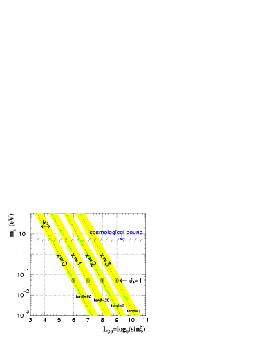
Figure 2.3: Tree-level neutrino mass dependence on $\log_{\theta}\sin\xi\approx L_{30}$ for different assignments of the charge difference $L_{30}=L_{3}-L_{0}$ and for different values of $\tan\beta$. Details in the text.

Let us introduce the parameterization

$$|n_{i}-n_{0}|-(5+x)=\delta_{i}\,.$$

Without loss of generality, we can also assume $n_{1}\leq n_{2}\leq n_{3}$ which implies

$$m_{\nu}^{\rm tree}\approx\theta^{\,2\delta_{3}}\>{\rm eV}\,.$$

It is worth stressing that the parameter that controls the scaling of $m_{\nu}^{\rm tree}$ with respect to changes in the values of the horizontal charges is $\theta^{\,2}\simeq 0.05\,$, and thus neutrino masses are much more sensitive to the horizontal symmetry than the other fermion masses that scale with $\theta$. For example $\delta_{3}=-1$ yields $m_{\nu}^{\rm tree}\sim 20\,$eV; $\delta_{3}=0$ yields $m_{\nu}^{\rm tree}\sim 1\,$eV; for $\delta_{3}=1$ all the trilinear $L$ violating couplings are forbidden, and at the same time $m_{\nu}^{\rm tree}\sim 5\times 10^{-2}\,$ eV (see Fig. 1) is in the correct range for a solution to the atmospheric neutrino problem [26, 143, 144]; finally, $\delta_{3}=2$ would suppress $m_{\nu}^{\rm tree}$ too much to allow for such a solution.

Let us now write the down-quarks and lepton Yukawa matrices as

$$h^{D}_{jk} \simeq \theta^{L_{0}+Q_{j}+d_{k}}=\theta^{Q_{j3}+d_{k3}+x}\,,\qquad$$

$$h^{E}_{jk} \simeq \theta^{L_{0}+L_{j}+e_{k}}=\theta^{L_{j3}+e_{k3}+x}\,,$$

where $x=L_{0}+Q_{3}+d_{3}=L_{0}+L_{3}+e_{3}\,$ consistently with our parameterization of $\tan\beta$ and with the approximate equality between the bottom and tau masses at sufficiently high energies (which in particular allows for $b$–$\tau$ Yukawa unification). The order of magnitude of the trilinear $L$ violating couplings is then:

$$\lambda^{\prime}_{ijk} \simeq \theta^{n_{i}-n_{0}}\,h^{d}_{jk}\simeq\theta^{Q_{j3}+d_{k3}-(5+\delta_{i})}\,,$$

$$\lambda_{ijk} \simeq \theta^{n_{i}-n_{0}}\,h^{l}_{jk}\simeq\theta^{L_{j3}+e_{k3}-(5+\delta_{i})}\,.$$ (2.24)

One can show that the phenomenological information on the charged fermion mass ratios and quark mixing angles can be re-expressed in terms of the sets of eight charge differences given in Table 2.3 [40, 116, 149, 150, 151]. Consequently gives rise to eight conditions on the fermion charges

model	$Q_{13}$	$Q_{23}$	$d_{13}$	$d_{23}$	$u_{13}$	$u_{23}$	model	$L_{13}+e_{13}$	$L_{23}+e_{23}$
MQ1:	3	2	1	0	5	2	ML1:	5	2
MQ2:	–3	2	7	0	11	2	ML2:	9	–2

Table 2.3: Models of horizontal charge differences

The phenomenological analysis leading to these sets of charge differences has been extensively discussed in the literature [40, 116, 149, 150, 151].

In [50] was shown that in the framework of models of Abelian horizontal symmetries, the phenomenological information on the charged fermion mass ratios and quark mixing angles expressed in terms of the eight horizontal charge differences in Tab. (2.3), when complemented with the requirement that $m_{\nu}^{\rm tree}$ is adequately suppressed below the eV scale ($\delta_{i}\geq 1$) hints at one self-consistent model (MQ1+ML1) where all the $\lambda$ and $\lambda^{\prime}$ couplings vanish. It is interesting to note that $\delta_{3}=1$ which yields $m_{\nu}^{\rm tree}\approx\theta^{2}$ eV in the correct range required by the atmospheric neutrino problem is also the minimum value that ensures $\lambda=0\,$, $\lambda^{\prime}=0$ and, as we will below, $\lambda^{\prime\prime}=0\,$.

Concerning MQ2 either the neutrino masses are uninterestingly small there, or the $\lambda^{\prime}$ conflicts with existing experimental limits. MQ2 is also excluded by the requirement that the $\lambda^{\prime\prime}$ couplings vanish

In ML2, once we set $L_{23}=0$ to allow for maximal $\nu_{\mu}$–$\nu_{\tau}$ mixing, the lepton mass ratios can be correctly reproduced only if $L_{12}\geq 4\,$, which would again exclude the possibility of explaining the solar neutrinos deficit through $\nu_{e}$–$\nu_{\mu}$ oscillations.

In conclusion, our analysis results in the set of fields charge differences and of $n_{\alpha}=L_{\alpha}+H_{u}$ charge sums displayed in Tab. 2.4

$Q_{13}$	$Q_{23}$	$d_{13}$	$d_{23}$	$u_{13}$	$u_{23}$	$L_{13}$	$L_{23}$	$e_{13}$	$e_{23}$	$n_{i}$	$n_{0}$
3	2	1	0	5	2	0	0	5	2	$-7-x$	$-1$

Table 2.4: Final charge differences

If we further use the analysis of the neutrino loop effects we would have in addition the value $x=1$ (corresponding to $\tan\beta\approx 10$–$40\,$). Of course, $x=0$ implies that the value of $\tan\beta$ is very large ($\sim 60$) and therefore this case is phenomenological disfavored [152, 153]. Finally $x=2$ ($\tan\beta\sim 5$) would yield a too large suppression to the loop neutrino mass to be interesting for the solar neutrinos.

Models based on a single $U(1)_{H}$ Abelian factor are completely specified in terms of the horizontal charges of the SM fields. There are five charges for each fermion family plus two charges for the Higgs doublets, for a total of 17 charges that a priori can be considered as free parameters (the charge of the $U(1)_{H}$ breaking parameter $\theta$ is just a normalization factor). The 17 horizontal charges are constrained by eleven phenomenological conditions corresponding to the eight constraints in Table 2.3, the $m_{t}$ value, the condition $m_{b}\approx m_{\tau}$ at high energy and the preferred value for the solution of the $\mu_{0}$ problem $n_{0}=-1$. Also by two theoretical conditions from anomaly cancellation through the GS mechanism. This leaves us with four free parameters, and we can chose them to be the charges $n_{i}$ ($i=1,2,3$) of the bilinear terms $\mu_{i}$, and $x=Q_{3}+d_{3}+L_{0}$ that fixes the value of $\tan\beta\,$. The expressions of the horizontal charges for all the SM fields as a function of these four parameters is given in the Appendix A. Then the self-consistent solution given in Table 2.4 is used to find the 17 individual charges presented in Table A.1. In the present case the Kähler contributions to the trilinear couplings are of order $m_{3/2}/M_{p}$ and powers of $\theta$ depending on the horizontal charges of the various dimension–4 terms. Moreover, for this set of individual charges the horizontal charges of $\lambda^{\prime\prime}$ are in addition fractional and consequently zero. In summary the resulting Dimension 4 and 5 $L$ and $B$ violating couplings in the basis where the horizontal charges are well defined are

$$\begin{split}\mu_{i}&=m_{3/2}\theta^{8},\qquad\lambda^{\prime}_{ijk}\approx(m_{3/2}/M_{p})\theta^{|L_{i}+Q_{j}+d_{k}|},\qquad\lambda_{ijk}\approx(m_{3/2}/M_{p})\theta^{|L_{i}+L_{j}+e_{k}|},\\ \lambda^{\prime\prime}_{ijk}&=0,\qquad\qquad\kappa^{\prime}_{ijkl}=0.\end{split}$$ (2.25)

This clearly define one SSSM.

In summary we have obtained one SSSM originating from an anomalous horizontal symmetry where the anomalies are canceled through a GS mechanism. We have assumed that all the superrenormalizable terms coupling the up-type Higgs doublet with the four hypercharge $-1/2$ doublets carry negative horizontal charges, and hence are forbidden by holomorphy. We have constrained the value of these charges by several theoretical and phenomenological requirements, such as having an acceptable Higgsino mass ($\mu$ problem) and neutrino masses suppressed below the electron-volt scale, as suggested by present neutrino data. We have found that under these conditions all the trilinear $L$ violating superpotential couplings vanish, yielding a SSSM which is defined by the charge differences in Tab. (2.4), where lepton number is mildly violated only by small bilinear terms. The model allows for neutrino masses in the correct ranges suggested by the atmospheric neutrino problem and by the LOW and quasi-vacuum solutions to the solar neutrino problem. However, no precise theoretical information can be obtained about the neutrino mixing angles except for the fact that, unlike the quark mixings, there is no parametric suppression of their values and thus they can be naturally large. Note that this model solves all the problems mentioned at the beginning of this chapter.

A similar mechanism but without the solution to the $\mu$ problem was implemented in [44]. In the example considered there the dimension–4 $L$ and $B$ violating operators are absent by holomorphy before the SUSY breaking. The dimension–4 $L$ and $B$ violating terms are generated from the Kähler potential and one get $\lambda^{\prime}\lambda^{\prime\prime}\sim 10^{-26}$. However the strength of the superrenormalizable term $\theta^{|-13|}$ is too small to be relevant in neutrino physics. The resulting individual charges for $\mu_{i}\approx m_{3/2}\theta^{|-6|}$ are shown in Table A.2 . The dimension–4 $L$ and $B$ violating terms satisfy now $\lambda^{\prime}\lambda^{\prime\prime}\lesssim 10^{-19}$.

2.4 Phenomenology of SSSM

The phenomenology of the SSSM has been extensively studied in literature. In particular:

• Neutralino-neutrino mixing: The tree level neutrino mass has been studied in [16, 18, 19, 100, 154, 155]. Analysis of one-loop neutrino masses and/or Solution to the neutrino anomalies can be found in [16, 88, 89, 94, 156, 157, 158, 159, 160, 161, 162, 163, 164, 165]. Numerical calculation with the full one-loop corrections: [34, 38]. An analytical study including the effect of arbitrary dimension–4 $L$ violating terms was performed in [96]. The neutrino spectrum in horizontal models have been estimated in [40, 44, 50, 89, 100, 126, 140, 158]

  Neutralino decays: [16, 19, 37, 41, 87, 88, 103, 166, 167]. Tevatron signatures of neutralino decay in [33]. Neutralino decay processes based on the assumption that the atmospheric neutrino masses and mixings are mainly due to the bilinear terms in [64]. In [16, 47] is concluded that the dominant decay of the neutralino is into $b\,\bar{b}$ quark jets and neutrino (or $b\,\bar{t}l^{+}$ if energetically allowed). In [33, 37, 61] it is shown that the decay of the lightest neutralino $\tilde{\chi}_{1}^{0}$ will produce comparable numbers of muons and taus as a result of the large mixing implied by the atmospheric anomaly. This result is also obtained in [34, 167]. Some of the neutralino decays channels for the one generation case were studied in [168]. The full numerical calculation of the neutralino decay in the one generation case was presented in [103], while the full numerical calculation in the three–generation case was presented in [167]. A systematic study of the SSSM including approximate formula for the neutralino–neutrino mixing was performed in [34, 99, 104, 167, 169]. In [170] it is shown that neutralino mix only with the heaviest neutrino in SSSM.

• Neutral Higgs – sneutrino mixing. Sneutrino production and/or decays have been studied in [41, 84, 87] and recently in [171]. Sneutrino mass splitting have been analyzed in [110, 171, 172]. An basis–independent analysis of this problem was performed in [173]. In [97] is studied the effect of $\widetilde{L}_{3}H_{u}$ term of the low energy scalar potential in the generation of spontaneous CP violation. Scalar resonance enhancement in $e^{+}e^{-}\to Z^{0}Z^{0}\,W^{+}W^{-}$ and in $e^{+}e^{-}\to t\bar{t}$ due two the sneutrino-Higgs mixing, have been recently studied in [174].

• Charged Higgs – stau mixing. Charged scalar decays have been studied in [85]

• Stop decays have been studied in [31, 70, 105, 106]

• Rare decays: $b\to s\gamma$ [91]; $Z^{0}$ decays as $Z^{0}\to\bar{\nu_{3}}\tilde{\chi}_{1}^{0}$ and $Z^{0}\to\tau^{+}\tilde{\chi}_{1}^{-}$ in [60, 107]; flavor changing coupling of the $W$ and $Z$ [87]; top decays [62]. The double beta decay have been studied in [104, 169, 175]. Proton decay in bilinear models were studied in [170, 176, 177]. In particular in [176, 177] the limit in eq. (2.3) translate into

  $$\frac{\mu_{i}}{\mu_{0}}\lambda^{\prime\prime}_{112}\lesssim 10^{-21}$$ (2.26)

  which is important in SSSM where the dimension–4 $B$ violating couplings are generated from the Kähler potential without further suppression, $\lambda^{\prime\prime}_{ijk}\lesssim\Lambda_{ijk}m_{3/2}/M_{p}$ ($j=1,2$). $\mu\to e\gamma$ and the numerical study of misalignment [98]. $\mu\to e\gamma$ and other rare processes [18, 19, 178]. Leptonic phenomenology and constraints [179].

• Others: Effects with large neutrino mass: [108]. SSSM in gauge mediated SUSY: [46, 64, 158, 180]. Fermion dipole moment: [181]. Magnetic moment of the neutrino [182].

• Spontaneous breaking of R-parity. In addition to the papers quoted in Section 2.2.1, the phenomenology of this models have been studied in [55, 56, 57, 70, 183, 184]

Chapter 3 The mass spectrum of the SSSM

Here we discuss the tree level structure of the supersymmetric masses and mixing of SSSM, discussing the fermion (chargino, neutralino) and scalar (squarks, sleptons and Higgs) mass matrices

3.1 Chargino mass matrix

In the SSSM the charginos mix with the charged leptons forming a set of five charged fermions $F_{i}^{\pm}$, $i=1,\ldots,5\,$ in two component spinor notation. In a basis where ${\psi^{+}}^{T}=[-i\lambda^{+},\widetilde{H}_{u}^{+},e_{R}^{+},\mu_{R}^{+},\tau_{R}^{+}]$, the mass terms in the lagrangian are

$$\mathcal{L}_{SSSM}=-\frac{1}{2}\begin{bmatrix}{\psi^{+}}^{T}&{\psi^{-}}^{T}\end{bmatrix}\begin{bmatrix}\mathbf{0}&\mathbf{M_{C}}^{T}\\ \mathbf{M_{C}}&\mathbf{0}\end{bmatrix}\begin{bmatrix}\psi^{+}\\ \psi^{-}\end{bmatrix}+\textrm{h.c}+\cdots$$

where the chargino/lepton mass matrix is given by [34]

$$\mathbf{M_{C}}=\begin{bmatrix}M_{2}&{\textstyle\frac{1}{\sqrt{2}}}gv_{u}&0\\ {\textstyle\frac{1}{\sqrt{2}}}gv_{0}&\mu_{0}&-{\textstyle\frac{1}{\sqrt{2}}}\sum_{j}h^{E}_{ij}v_{j}\\ {\textstyle\frac{1}{\sqrt{2}}}gv_{k}&\mu_{k}&{\textstyle\frac{1}{\sqrt{2}}}\mathbf{h^{E}}v_{0}\end{bmatrix}$$ (3.1)

where the index $i$ expands over the columns and $k$ labels the rows. We note that the chargino sector decouples from the leptonic sector in the limit $\mu_{i}=v_{i}=0$. As in the MSSM, the chargino mass matrix is diagonalized by two rotation matrices $\mathbf{U}$ and $\mathbf{V}$

$${\bf U}^{*}{\bf M_{C}}{\bf V}^{-1}=\mathrm{diag}\left(m_{\tilde{\chi}^{\pm}_{i}},m_{e_{i}}\right)=\mathrm{diag}\left(m_{\tilde{F}^{\pm}_{a}}\right)\qquad a=1,\ldots,5$$ (3.2)

where $i=1,2$ for the charginos, and $j=1,2,3$ for the neutrinos.

In the one generation case, the composition of the tau is given by

$$\tau^{+}_{R}=V_{3j}\psi_{j}^{+},\qquad\tau^{-}_{L}=U_{3j}\psi_{j}^{-}$$ (3.3)

where $\psi^{+T}=(-i\lambda^{+},\widetilde{H}_{u}^{1},\tau_{R}^{0+})$ and $\psi^{-T}=(-i\lambda^{-},\widetilde{L}_{0}^{2},\tau_{L}^{0-})$. The two-component Weyl spinors $\tau_{R}^{0-}$ and $\tau_{L}^{0+}$ are weak eigenstates, while $\tau^{+}_{R}$ and $\tau^{-}_{L}$ are the mass eigenstates. It follows easily from eq. (3.2) that the matrix ${\bf{M_{C}M_{C}^{T}}}$ is diagonalized by ${\bf U}$ and the matrix ${\bf{M_{C}^{T}M_{C}}}$ is diagonalized by ${\bf V}$.

3.2 Neutralino mass matrix

In the basis ${\psi^{0}}^{T}=[-i\lambda^{\prime},-i\lambda^{3},\widetilde{H}_{u}^{0},\widetilde{H}_{d}^{0},\nu_{e},\nu_{\mu},\nu_{\tau}]\,$ the neutral fermion mass matrix $\mathbf{M_{N}}$ is given by [34]:

$$\mathbf{M_{N}}=\begin{bmatrix}M_{1}&0&\frac{1}{2}\,g^{\prime}\,v_{u}&-\frac{1}{2}\,g^{\prime}\,\mathbf{v}\\ 0&M_{2}&-\frac{1}{2}\,g\,v_{u}&\frac{1}{2}\,g\,\mathbf{v}\\ \frac{1}{2}\,g^{\prime}\,v_{u}&-\frac{1}{2}\,g\,v_{u}&0&-\boldsymbol{\mu}\\ -\frac{1}{2}\,g^{\prime}\,\mathbf{v}^{T}&\frac{1}{2}\,g\,\mathbf{v}^{T}&-\boldsymbol{\mu}^{T}&0\\ \end{bmatrix}$$ (3.4)

where $\mathbf{v}$ ($\boldsymbol{\mu}$) is the vector defined by $v_{\alpha}$ ($\mu_{\alpha}$). This matrix is diagonalized by a $7\times 7$ unitary matrix $N$,

$$N^{*}\,\mathbf{M_{N}}\,N^{-1}=\mathrm{diag}\left(m_{\tilde{\chi}_{i}^{0}},m_{\nu_{j}}\right)=\mathrm{diag}\left(m_{\tilde{F}_{a}^{0}}\qquad a=1,\ldots,7\right)$$ (3.5)

where $i=1,\cdots,4$ for the neutralinos, and $j=1,\cdots,3$ for the neutrinos.

3.3 The squark mass spectrum

The up and down-type squark mass matrices of our model have already been given previously in Ref. [95]. Here we generalize those to the three-generation case [31]. The mass matrix of the up squark sector follows from the quadratic terms in the scalar potential

$$V_{\mathrm{quadratic}}=\begin{bmatrix}\tilde{\mathbf{u}}_{L}^{\dagger}&\tilde{\mathbf{u}}_{R}^{\dagger}\end{bmatrix}\mathbf{{\tilde{M}_{U}^{2}}}\begin{bmatrix}\tilde{\mathbf{u}}_{L}\\ \tilde{\mathbf{u}}_{R}\end{bmatrix}+\cdots$$ (3.6)

given by

$$\mathbf{\tilde{M}_{U}^{2}}=\begin{bmatrix}{\mathbf{M_{Q}^{2}}}+\frac{1}{2}v_{u}^{2}{\mathbf{h_{U}}}{\mathbf{h_{U}}}^{\dagger}+\boldsymbol{\Delta}_{UL}&\frac{1}{\sqrt{2}}v_{u}{\mathbf{A_{U}^{h}}}-\frac{1}{\sqrt{2}}(\mu_{0}v_{0}+\mu_{3}v_{3}){\mathbf{h_{U}}}\\ \frac{1}{\sqrt{2}}v_{u}{\mathbf{A_{U}^{h}}}^{\dagger}-\frac{1}{\sqrt{2}}(\mu_{0}v_{0}+\mu_{3}v_{3}){\mathbf{h_{U}}}^{\dagger}&{\mathbf{M_{U}^{2}}}+\frac{1}{2}v_{u}^{2}{\mathbf{h_{U}}}^{\dagger}{\mathbf{h_{U}}}+\boldsymbol{\Delta}_{UR}\end{bmatrix}$$ (3.7)

where $\boldsymbol{\Delta}_{UL}=\frac{1}{8}\big{(}g^{2}-\frac{1}{3}{g^{\prime}}^{2}\big{)}\big{(}v_{0}^{2}-v_{u}^{2}+v_{3}^{2}\big{)}\mathbf{1}$ and $\boldsymbol{\Delta}_{UR}=\frac{1}{6}{g^{\prime}}^{2}(v_{0}^{2}-v_{u}^{2}+v_{3}^{2})\mathbf{1}$ are the splitting in the squark mass spectrum produced by electro-weak symmetry breaking, and ${A_{U}^{h}}_{ij}\equiv A_{U}^{ij}h_{U}^{ij}$. The eigenvalues of $\mathbf{\tilde{M}_{U}^{2}}$ are

$$\textrm{diag}\,\{m_{\tilde{u}_{1}},m_{\tilde{u}_{2}},\ldots,m_{\tilde{u}_{6}}\}=\begin{bmatrix}\boldsymbol{\Gamma}_{UL}&\boldsymbol{\Gamma}_{UR}\end{bmatrix}\mathbf{\tilde{M}_{U}^{2}}\begin{bmatrix}\boldsymbol{\Gamma}_{UL}^{\dagger}\\ \boldsymbol{\Gamma}_{UR}^{\dagger}\end{bmatrix}$$ (3.8)

This way the six weak-eigenstate fields $\tilde{u}_{iL}$ and $\tilde{u}_{iR}$ ($i=1,2,3$) combine into six up-type mass eigenstate squarks $\tilde{u}_{k}$ as follows: $\tilde{u}_{iL}=\Gamma^{\dagger ik}_{UL}\tilde{u}_{k}=\Gamma^{*ki}_{UL}\tilde{u}_{k}$, $\tilde{u}_{iR}=\Gamma^{\dagger ik}_{UR}\tilde{u}_{k}=\Gamma^{*ki}_{UR}\tilde{u}_{k}$.

For completeness, we also give the mass matrix of the down squark sector. The quadratic scalar potential includes

$$V_{\mathrm{quadratic}}=\begin{bmatrix}\tilde{\mathbf{d}}_{L}^{*}&\tilde{\mathbf{d}}_{R}^{*}\end{bmatrix}\mathbf{\tilde{M}_{D}^{2}}\begin{bmatrix}\tilde{\mathbf{d}}_{L}\\ \tilde{\mathbf{d}}_{R}\end{bmatrix}+\cdots$$ (3.9)

given by

$$\mathbf{\tilde{M}_{D}^{2}}=\begin{bmatrix}\mathbf{M_{Q}^{2}}+\frac{1}{2}v_{0}^{2}\mathbf{h_{D}}\mathbf{h_{D}}^{\dagger}+\boldsymbol{\Delta}_{DL}&\frac{1}{\sqrt{2}}v_{0}\mathbf{A_{D}^{h}}-\frac{1}{\sqrt{2}}\mu_{0}v_{u}\mathbf{h_{D}}\\ \frac{1}{\sqrt{2}}v_{0}\mathbf{A_{D}^{h}}^{\dagger}-\frac{1}{\sqrt{2}}\mu_{0}v_{u}\mathbf{h_{D}}^{\dagger}&\mathbf{M_{D}^{2}}+\frac{1}{2}v_{0}^{2}\mathbf{h_{D}}^{\dagger}\mathbf{h_{D}}+\boldsymbol{\Delta}_{DR}\end{bmatrix}$$ (3.10)

where $\boldsymbol{\Delta}_{DL}=-\frac{1}{8}\big{(}g^{2}+\frac{1}{3}{g^{\prime}}^{2}\big{)}\big{(}v_{0}^{2}-v_{u}^{2}+v_{3}^{2}\big{)}\mathbf{1}$, $\boldsymbol{\Delta}_{DR}=-\frac{1}{12}{g^{\prime}}^{2}(v_{0}^{2}-v_{u}^{2}+v_{3}^{2})\mathbf{1}$, and ${A_{D}^{h}}_{ij}\equiv A_{D}^{ij}h_{D}^{ij}$. The eigenvalues of $\mathbf{\tilde{M}_{D}^{2}}$ are

$$\textrm{diag}\,\{m_{\tilde{d}_{1}},m_{\tilde{d}_{2}},\ldots,m_{d_{6}}\}=\begin{bmatrix}\boldsymbol{\Gamma}_{DL}&\boldsymbol{\Gamma}_{DR}\end{bmatrix}\mathbf{\tilde{M}_{D}^{2}}\begin{bmatrix}\boldsymbol{\Gamma}_{DL}^{\dagger}\\ \boldsymbol{\Gamma}_{DR}^{\dagger}\end{bmatrix}$$ (3.11)

One is left with six mass-eigenstate down squarks fields $\tilde{d}_{k}$ related to $\tilde{d}_{iL}$ and $\tilde{d}_{iR}$ fields as follows: $\tilde{d}_{iL}=\Gamma^{\dagger ik}_{DL}\tilde{d}_{k}=\Gamma^{*ki}_{DL}\tilde{d}_{k}$, $\tilde{d}_{iR}=\Gamma^{\dagger ik}_{DR}\tilde{d}_{k}=\Gamma^{*ki}_{UR}\tilde{d}_{k}$.

3.4 Scalar Mass Matrices

The electroweak symmetry is broken when the Higgs and slepton fields acquire non–zero vevs. These are calculated via the minimization of the effective potential or, in the diagrammatic method, via the tadpole equations. The full scalar potential at tree level is

$$V_{\mathrm{total}}^{0}=\sum_{i}\left|\frac{\partial W}{\partial z_{i}}\right|^{2}+V_{D}+V_{\mathrm{soft}}^{\mathrm{MSSM}}+V_{\mathrm{soft}}^{\mathrm{SSSM}}$$ (3.12)

where $z_{i}$ is any of the scalar fields in the superpotential in eq. (1.33), $V_{D}$ are the $D$-terms, and $V_{\mathrm{soft}}^{\mathrm{SSSM}}$ is the $L$ violating part of eq. (1.21)

The tree level scalar potential contains the following linear terms

$$V_{\mathrm{linear}}^{0}=t_{d}^{0}\sigma^{0}_{d}+t_{u}^{0}\sigma^{0}_{u}+t_{1}^{0}\tilde{\nu}^{R}_{1}+t_{2}^{0}\tilde{\nu}^{R}_{2}+t_{3}^{0}\tilde{\nu}^{R}_{3}\,,$$ (3.13)

where the different $t^{0}$ are the tadpoles at tree level. They are given by

$$\begin{split}t_{u}^{0}&=-\textstyle{\frac{1}{2}}v_{\beta}(B_{\beta\gamma}+B_{\gamma\beta})\mu_{\gamma}+\Big{[}m_{H_{u}}^{2}+\mu_{\beta}\mu_{\beta}-\textstyle{\frac{1}{8}}(g^{2}+{g^{\prime}}^{2})(v_{\beta}v_{\beta}-v_{u}^{2})\Big{]}v_{u}\\ t_{\alpha}^{0}&=\textstyle{\frac{1}{8}}(g^{2}+{g^{\prime}}^{2})(v_{\beta}v_{\beta}-v_{u}^{2})v_{\alpha}+\mu_{\alpha}\mu_{\beta}v_{\beta}-\textstyle{\frac{1}{2}}(B_{\alpha\beta}+B_{\beta\alpha})\mu_{\beta}v_{u}+{\textstyle\frac{1}{2}}(M^{2}_{L\alpha\beta}+M^{2}_{L\beta\alpha})v_{\beta}\end{split}$$ (3.14)

Repeated indexes $\beta,\gamma$ in eq. (3.14) implies summation over $0,1,2,3$. The five tree level tadpoles are equal to zero at the minimum of the tree level potential.

We assume that non–diagonal $M_{L_{ij}}^{2}$ soft parameters are negligible. Therefore we further denote $M_{L_{ii}}^{2}$ as $M_{L_{i}}^{2}$

The quadratic scalar potential includes [85, 105].

$$V_{quadratic}=\begin{bmatrix}H_{d}^{-}&H_{u}^{-}&\tilde{e}_{iL}^{-}&\tilde{e}_{iR}^{-}\end{bmatrix}\mathbf{M_{S^{\pm}}^{2}}\begin{bmatrix}H_{d}^{+}\\ H_{u}^{+}\\ \tilde{e}_{iL}^{+}\\ \tilde{e}_{iR}^{+}\\ \end{bmatrix}\\ +{\textstyle\frac{1}{2}}\left[\begin{array}[]{ccc}\sigma^{0}_{d}&\sigma^{0}_{u}&\tilde{\nu}_{i}^{R}\end{array}\right]\mathbf{M^{2}_{S^{0}}}\left[\begin{array}[]{c}\sigma^{0}_{d}\\ \sigma^{0}_{u}\\ \tilde{\nu}_{i}^{R}\end{array}\right]+{\textstyle\frac{1}{2}}\left[\begin{array}[]{ccc}\varphi^{0}_{1}&\varphi^{0}_{2}&\tilde{\nu}_{i}^{I}\end{array}\right]{\mathbf{M^{2}_{P^{0}}}}\left[\begin{array}[]{c}\varphi^{0}_{1}\\ \varphi^{0}_{2}\\ \tilde{\nu}_{i}^{I}\end{array}\right]+\cdots$$ (3.15)

We will denote the physical scalar bosons by $S^{0}_{i}$, the pseudo-scalar by $P^{0}_{i}$ and the charged bosons by $S^{\pm}_{i}$. Higgs bosons mix with charged sleptons and the real (imaginary) parts of the sneutrino mix with the scalar (pseudoscalar) Higgs bosons. The mass matrices in eq. (3.15), will be given in following subsections.

3.4.1 Charged scalars

The mass matrix of the charged scalar sector follows from the quadratic terms in the scalar potential in eq. (3.15). For convenience reasons we will divide this $8\times 8$ charged scalar mass matrix into blocks in the following way:

$$\mathbf{M_{S^{\pm}}^{2}}=\left[\begin{array}[]{ccc}\mathbf{M_{HH}^{2}}&\mathbf{M_{H\tilde{\ell}}^{2}}^{T}\\ \mathbf{M_{H\tilde{\ell}}^{2}}&\mathbf{M_{\tilde{\ell}\tilde{\ell}}^{2}}\end{array}\right]\,.$$ (3.16)

Using the tadpole equations given in eqs. (3.14) we obtain (sum upon repeated indices):

$$\begin{split}&\mathbf{M_{HH}^{2}}=\\ &\left[\begin{array}[]{ccc}\!\!B_{0}\mu_{0}{\frac{v_{u}}{v_{0}}}+{\textstyle\frac{1}{4}}g^{2}(v_{u}^{2}-v_{i}v^{i})-\mu_{0}\mu_{i}{\frac{v^{i}}{v_{0}}}+{\textstyle\frac{1}{2}}v^{i}(\mathbf{h^{E}}\mathbf{h^{E}}^{{\dagger}})_{ij}v^{j}&B_{0}\mu_{0}+{\textstyle\frac{1}{4}}g^{2}v_{0}v_{u}\\ B_{0}\mu_{0}+{\textstyle\frac{1}{4}}g^{2}v_{0}v_{u}&B_{0}\mu_{0}{\frac{v_{0}}{v_{u}}}+{\textstyle\frac{1}{4}}g^{2}(v_{0}^{2}+v_{i}v^{j})+B_{i}\mu_{i}{\frac{v^{i}}{v_{u}}}\end{array}\right]\end{split}$$

This matrix reduces to the usual charged Higgs mass matrix in the MSSM when we set $v_{i}=\mu_{i}=0$. The slepton block is given by

$$\mathbf{M_{\tilde{\ell}\tilde{\ell}}^{2}}=\begin{bmatrix}\mathbf{M_{LL}^{2}}&\mathbf{M_{LR}^{2}}\\ \mathbf{M_{RL}^{2}}&\mathbf{M_{RR}^{2}}\\ \end{bmatrix}$$

$$\begin{split}\left(\mathbf{M_{LL}^{2}}\right)_{ij}=&\frac{1}{2}\,v_{o}^{2}(\mathbf{h_{E}}^{*}\mathbf{h_{E}}^{T})_{ij}+\frac{1}{4}\,g^{2}\left(v_{u}^{2}-\textstyle{\sum_{\alpha}}v_{\alpha}^{2}\right)\delta_{ij}+\frac{1}{4}\,g^{2}v_{i}v_{j}-\frac{v_{u}}{v_{i}}B_{i}\epsilon_{i}\delta_{ij}\\ &-\mu_{i}\frac{\sum_{\alpha}v_{\alpha}\mu_{\alpha}}{v_{i}}\,\delta_{ij}+\mu_{i}\mu_{j}+{M_{L}^{2}}_{ji}-\frac{1}{2}\sum_{k}\frac{v_{k}}{v_{i}}\left({M^{2}_{L}}_{ik}+{M^{2}_{L}}_{ki}\right)\delta_{ij}\\ \mathbf{M_{LR}^{2}}=&\frac{1}{\sqrt{2}}\left(v_{0}\mathbf{A_{E}^{h}}^{*}-\mu_{0}v_{u}\mathbf{h_{E}}^{*}\right)\\ \mathbf{M_{RL}^{2}}=&\mathbf{M_{LR}^{2}}^{{\dagger}}\\ \left(\mathbf{M_{RR}^{2}}\right)_{ij}=&\frac{1}{4}\,{g^{\prime}}^{2}\left(-\textstyle{\sum_{\alpha}}v_{\alpha}^{2}+v_{u}^{2}\right)\delta_{ij}+\frac{1}{2}\,\textstyle{\sum_{\alpha}}v_{\alpha}^{2}\left(\mathbf{h_{E}}^{T}\mathbf{h_{E}}^{*}\right)_{ij}+{M_{E}^{2}}_{ji}\end{split}$$

where ${A_{E}^{h}}^{ij}=A_{E}^{ij}h_{E}^{ij}$.

The mixing between the charged Higgs sector and the stau sector is given by the following $6\times 2$ block:

$$\mathbf{M_{H\tilde{\ell}}^{2}}=\left[\begin{array}[]{ccc}\mu_{0}\mu_{i}-\frac{1}{2}v_{0}\sum_{k}(\mathbf{h_{E}}^{T}\mathbf{h_{E}}^{*})_{ik}v_{k}+\frac{1}{4}g^{2}v_{0}v_{i}&B_{i}\mu_{i}+\frac{1}{4}g^{2}v_{u}v_{i}\\ {\frac{1}{\sqrt{2}}}v_{u}\sum_{k}(\mathbf{h_{E}}^{T})_{ik}\mu_{k}-\frac{1}{\sqrt{2}}\textstyle{\sum}_{k}(\mathbf{A_{E}^{L}}^{T})_{ik}v_{k})&-{\frac{1}{\sqrt{2}}}\sum_{k}(\mathbf{h_{E}}^{T})_{ik}(\mu_{0}v_{k}-\mu_{k}v_{0})\end{array}\right]$$

The mass matrix in eqs. (3.16), is diagonalized by rotation matrices which define the eigenvectors

$$\mathbf{S^{+}}=\mathbf{R_{S^{\pm}}}\mathbf{{S^{\prime}}^{+}}$$

and the eigenvalues in the one generation case are

$$\rm{diag}(0,m_{S^{\pm}_{2}}^{2},m_{S^{\pm}_{3}}^{2},m_{S^{\pm}_{4}}^{2})=\mathbf{R_{S^{\pm}}}\mathbf{M_{S^{\pm}}^{2}}\mathbf{R_{S^{\pm}}^{T}}$$

3.4.2 CP–Even Neutral Scalars

The neutral CP-even scalar sector mass matrix in eq. (3.15) is given by

$$\mathbf{M_{S^{0}}^{2}}=\left[\begin{array}[]{cc}\mathbf{M_{SS}^{2}}&\mathbf{M_{S\widetilde{\nu}_{R}}^{2}}\\ \mathbf{M_{S\widetilde{\nu}_{R}}^{2}}^{T}&\mathbf{M_{\widetilde{\nu}_{R}\widetilde{\nu}_{R}}^{2}}\end{array}\right]$$ (3.17)

where

$$\mathbf{M_{SS}^{2}}=\left[\begin{array}[]{cc}\displaystyle B_{0}\mu_{0}\frac{v_{u}}{v_{0}}+{\textstyle\frac{1}{4}}g_{Z}^{2}v_{0}^{2}-\mu_{0}\sum_{k=1}^{3}\mu_{k}\frac{v_{k}}{v_{0}}+\frac{t_{d}}{v_{0}}&-B_{0}\mu_{0}-{\textstyle\frac{1}{4}}g^{2}_{Z}v_{0}v_{u}\\ -B_{0}\mu_{0}-{\textstyle\frac{1}{4}}g^{2}_{Z}v_{0}v_{u}&\displaystyle B_{0}\mu_{0}\frac{v_{0}}{v_{u}}+{\textstyle\frac{1}{4}}g^{2}_{Z}v_{u}^{2}+\sum_{k=1}^{3}\,B_{k}\mu_{k}\frac{v_{k}}{v_{u}}+\frac{t_{u}}{v_{u}}\end{array}\right]$$ (3.18)

$$\mathbf{M_{S\widetilde{\nu}_{R}}^{2}}=\left[\begin{array}[]{cc}\mu_{0}\mu_{i}+{\textstyle\frac{1}{4}}g^{2}_{Z}v_{0}v_{i}\\ -B_{i}\mu_{i}-{\textstyle\frac{1}{4}}g^{2}_{Z}v_{u}v_{i}\end{array}\right]$$

and

$$\left(\mathbf{M_{\widetilde{\nu}_{R}\widetilde{\nu}_{R}}^{2}}\right)_{ij} =\left(-\mu_{0}\mu_{i}\frac{v_{0}}{v_{i}}+B_{i}\mu_{i}\frac{v_{u}}{v_{i}}-\mu_{i}\sum_{k=1}^{3}\mu_{k}\frac{v_{k}}{v_{i}}-{\textstyle\frac{1}{2}}\sum_{k=1}^{3}\frac{v_{k}}{v_{i}}\left(M^{2}_{Lik}+M^{2}_{Lki}\right)+\frac{t_{i}}{v_{i}}\right)\delta_{ij}$$

$$+{\textstyle\frac{1}{4}}g^{2}_{Z}v_{i}v_{j}+\mu_{i}\mu_{j}+{\textstyle\frac{1}{2}}\left(M^{2}_{Lij}+M^{2}_{Lji}\right)$$ (3.19)

where we have defined $g_{Z}^{2}\equiv g^{2}+{g^{\prime}}^{2}$. In the upper–left $2\times 2$ block, in the limit $v_{i}=\mu_{i}=0$, the reader can recognize the MSSM mass matrix corresponding to the CP–even neutral Higgs sector. To define the rotation matrices let us define the unrotated fields by

$$\mathbf{{S^{\prime}}^{0}}=\left[\begin{array}[]{ccccc}\sigma_{d}^{0}&\sigma_{u}^{0}&\widetilde{\nu}_{1}^{R}&\widetilde{\nu}_{2}^{R}&\widetilde{\nu}_{2}^{R}\end{array}\right]$$ (3.20)

Then the mass eigenstates are $S^{0}_{i}$ given by

$$S^{0}_{i}={R}^{S^{0}}_{ij}{S^{\prime}}^{0}_{j}$$ (3.21)

with the eigenvalues $\mathrm{diag}(m^{2}_{S_{1}},\ldots,m^{2}_{S_{5}})=\mathbf{R^{S^{0}}}\,\mathbf{M_{S^{0}}^{2}}\,\left(\mathbf{R^{S^{0}}}\right)^{T}$.

3.4.3 CP–Odd Neutral Scalars

The quadratic scalar potential includes

where the CP-odd neutral scalar mass matrix is

$$\mathbf{M_{P^{0}}^{2}}=\left[\begin{array}[]{cc}\mathbf{M_{PP}^{2}}&\mathbf{M_{P\widetilde{\nu}_{I}}^{2}}\\ \mathbf{M_{P\widetilde{\nu}_{I}}^{2}}^{T}&\mathbf{M_{\widetilde{\nu}_{I}\widetilde{\nu}_{I}}^{2}}\end{array}\right]$$ (3.22)

where

$$\mathbf{M_{PP}^{2}}=\left[\begin{array}[]{cc}\displaystyle B_{0}\mu_{0}\frac{v_{u}}{v_{0}}-\mu_{0}\sum_{k=1}^{3}\mu_{k}\frac{v_{k}}{v_{0}}+\frac{t_{d}}{v_{0}}&B_{0}\mu_{0}\\ B_{0}\mu_{0}&\displaystyle B_{0}\mu_{0}\frac{v_{0}}{v_{u}}+\sum_{k=1}^{3}B_{k}\mu_{k}\frac{v_{k}}{v_{u}}+\frac{t_{u}}{v_{u}}\end{array}\right]$$ (3.23)

Note that in the limit $\mu_{0}\to 0$ a Goldstone boson appear.

$$\mathbf{M_{P\widetilde{\nu}_{I}}^{2}}=\left[\begin{array}[]{c}\mu_{0}\mu_{i}\\ B_{i}\mu_{i}\end{array}\right]$$

and

$$\left(\mathbf{M_{\widetilde{\nu}_{I}\widetilde{\nu}_{I}}^{2}}\right)_{ij} =\left(-\mu_{0}\mu_{i}\frac{v_{0}}{v_{i}}+B_{i}\mu_{i}\frac{v_{u}}{v_{i}}-\mu_{i}\sum_{k=1}^{3}\mu_{k}\frac{v_{k}}{v_{i}}-{\textstyle\frac{1}{2}}\sum_{k=1}^{3}\frac{v_{k}}{v_{i}}\left(M^{2}_{Lik}+M^{2}_{Lki}\ \right)+\frac{t_{i}}{v_{i}}\right)\delta_{ij}$$

$$+\mu_{i}\mu_{j}+{\textstyle\frac{1}{2}}\left(M^{2}_{Lij}+M^{2}_{Lji}\right)$$ (3.24)

The neutral pseudo–scalar mass matrices are diagonalized by the following rotation matrices,

$$P_{i}={R}^{P^{0}}_{ij}P^{\prime}_{j}$$ (3.25)

with the eigenvalues $\mathrm{diag}(m^{2}_{A_{1}},\ldots,m^{2}_{A_{5}})=\mathbf{R^{P^{0}}}\,\mathbf{M_{P^{0}}^{2}}\,\left(\mathbf{R^{P^{0}}}\right)^{T}$, where the unrotated fields are

$$\mathbf{{P^{\prime}}^{0}}=\left[\begin{array}[]{ccccc}\varphi_{d}^{0}&\varphi_{u}^{0}&\widetilde{\nu}_{1}^{I}&\widetilde{\nu}_{2}^{I}&\widetilde{\nu}_{2}^{I}\end{array}\right]$$ (3.26)

May be convenient some times take the pseudoscalar mass eigenvalues as input, it is worth briefly repeating here the discussion of the pseudoscalar bosons masses. The pseudo-scalar mass matrix in the one generation case is given by by:

$$\mathbf{M^{2}_{P^{0}}}=\left[\begin{array}[]{ccc}B_{0}\mu_{0}{\frac{v_{u}}{v_{0}}}-\mu_{0}\mu_{3}{\frac{v_{3}}{v_{0}}}&B_{0}\mu_{0}&+\mu_{0}\mu_{3}\\ B_{0}\mu_{0}&B_{0}\mu_{0}{\frac{v_{0}}{v_{u}}}+B_{3}\mu_{3}{\frac{v_{3}}{v_{u}}}&+B_{3}\mu_{3}\\ +\mu_{0}\mu_{3}&+B_{3}\mu_{3}&-\mu_{0}\mu_{3}{\frac{v_{0}}{v_{3}}}+B_{3}\mu_{3}{\frac{v_{u}}{v_{3}}}\end{array}\right]\,.$$ (3.27)

As expected, this matrix has zero determinant, since the neutral Goldstone boson eaten by the $Z$ is one of the corresponding states. Therefore, the masses of the two physical states are given by the formula:

$$m_{2,3}={\frac{1}{2}}{\rm Tr}\mathbf{M}\pm{\frac{1}{2}}\sqrt{\left({\rm Tr}\mathbf{M}\right)^{2}-4(M_{11}M_{22}-M_{12}^{2}+M_{11}M_{33}-M_{13}^{2}+M_{22}M_{33}-M_{23}^{2})}.$$ (3.28)

Therefore we can easily take one these masses as input and calculate $B_{0}\mu_{0}$ from it using

$$B_{0}\mu_{0}=\frac{-m_{P^{0}_{2}}^{4}v_{0}v_{u}v_{3}+B_{3}\mu_{3}\mu_{0}v_{3}(v_{0}^{2}+v_{u}^{2}+v_{3}^{2})+\mu_{3}m_{P^{0}_{2}}^{2}[\mu_{0}v_{u}(v_{0}^{2}+v_{3}^{2})]-B_{3}v_{0}(v_{u}^{2}+v_{3}^{2})}{-m_{P^{0}_{2}}^{2}(v_{0}^{2}+v_{u}^{2})v_{3}+\mu_{3}(\mu_{0}v_{0}-B_{3}v_{u})(v_{0}^{2}+v_{u}^{2}+v_{3}^{2})}$$

$B_{3}$ is obtained from the minimum equation for given $\mu_{3}$ and $v_{3}$ [85].

Chapter 4 Sparticle decays

4.1 Decays of neutralinos

If unprotected by the ad hoc assumption of R–parity conservation the LSP will decay as a result of gauge boson, squark, slepton and Higgs boson exchanges.

Although for the discussion of flavor–changing processes, such as neutrino oscillations involving all three generations, it is important to consider the full three-generation structure of the model, for the following discussion of neutralino decay properties it will suffice to assume $L$ violation only in the third generation, as a first approximation.

The relevant contributions to these decays are given in Table 1. The Feynman diagrams for the decays not involving taus, i.e. $\tilde{\chi}^{0}_{1}\to\nu_{3}f\bar{f}$ ($f=e$, $\nu_{e}$, $\mu$, $\nu_{\mu}$, $u$, $d$, $c$, $s$, $b$) are shown explicitly in Fig. 4.1.

Figure 4.1: Feynman graphs for the decay $\tilde{\chi}^{0}_{1}\to\nu_{3}\,f\,\bar{f}$ where $f\neq\tau$.

For this class of decays we have $Z^{0}$, $P^{0}_{i}$, and $S^{0}_{j}$ exchange in the direct channel (Fig. 4.1a and b) and $\tilde{f}$ exchange in the crossed channels (Fig. 4.1c and d). In particular in the case $f=b$ the $P^{0}_{i}$ and $S^{0}_{j}$ exchange contributions are significant. This is quite analogous to the results found in [185] for $\tilde{\chi}^{0}_{2}\to\tilde{\chi}^{0}_{1}f\bar{f}$ decays. The particles exchanged in the $s$-, $t$-, and $u$-channel for the decays $\tilde{\chi}^{0}_{1}\to\tau^{\pm}l^{\mp}\nu_{l}$, ($l=e,\mu$), $\tilde{\chi}^{0}_{1}\to\tau^{\pm}q\bar{q}^{\prime}$ ($q,q^{\prime}=u,d,s,c$), $\tilde{\chi}^{0}_{1}\to\tau^{-}\tau^{+}\nu_{l}$, and $\tilde{\chi}^{0}_{1}\to 3\nu_{3}$ are given in Tab. 4.1.

Decay mode	exchanged particle	channel
$\tilde{\chi}^{0}_{1}\to 3\,\nu_{3}$	$Z$, $S^{0}_{i}$, $P^{0}_{j}$	$s$
	$Z$, $S^{0}_{i}$, $P^{0}_{j}$	$t$
	$Z$, $S^{0}_{i}$, $P^{0}_{j}$	$u$
$\tilde{\chi}^{0}_{1}\to\nu_{3}\,\nu_{l}\,\bar{\nu}_{l}$ ($l=e,\mu$)	$Z$	$s$
	$\overline{\tilde{\nu}}_{l}$	$t$
	$\tilde{\nu}_{l}$	$u$
$\tilde{\chi}^{0}_{1}\to\nu_{3}\,f\,\bar{f}$ ($f=e,\mu,u,d,s,c,b$)	$Z$, $S^{0}_{i}$, $P^{0}_{j}$	$s$
	$\overline{\tilde{f}}_{1,2}$	$t$
	$\tilde{f}_{1,2}$	$u$
$\tilde{\chi}^{0}_{1}\to\nu_{3}\,\tau^{+}\,\tau^{-}$	$Z$, $S^{0}_{i}$, $P^{0}_{j}$	$s$
	$W^{-}$, $S^{-}_{k}$	$t$
	$W^{+}$, $S^{+}_{k}$	$u$
$\tilde{\chi}^{0}_{1}\to\nu_{l}\,\tau^{\pm}\,l^{\mp}$ ($l=e,\mu$)	$W^{\pm}$, $S^{\pm}_{k}$	$s$
	$\overline{\tilde{l}}_{1,2}$	$t$
	$\tilde{\nu}_{l}$	$u$
$\tilde{\chi}^{0}_{1}\to\tau\,q\,\bar{q}^{\prime}$ ($q=u,c$, $q^{\prime}=d,s$)	$W^{\pm}$, $S^{\pm}_{k}$	$s$
	$\overline{\tilde{q}}^{\prime}_{1,2}$	$t$
	$\tilde{q}_{1,2}$	$u$

Table 4.1: Contributions involved in the lightest neutralino 3-body decay modes. The $s$-, $t$-, and $u$-channels are defined by: $s=(p_{1}-p_{2})^{2}$, $t=(p_{1}-p_{3})^{2}$, and $u=(p_{1}-p_{4})^{2}$. See also Fig. 4.1.

In the calculations we have included all mixing effects, in particular the standard MSSM ${\tilde{f}}_{L}-{\tilde{f}}_{R}$ mixing effects and those induced by the bilinear $L$ violating terms, i.e. $Re(\tilde{\nu}_{3})-h^{0}-H^{0}$, $Im(\tilde{\nu}_{3})-A^{0}-G^{0}$, [84], ${\tilde{\tau}}_{L,R}^{\pm}-H^{\pm}-G^{\pm}$ [85], $\nu_{3}$ - $\tilde{\chi}^{0}_{i}$ [186], and $\tau$ - $\tilde{\chi}^{-}_{j}$ mixings [58, 59, 60]. These mixing effects are particularly important in the calculations of the various $L$ violating decay rates of $\tilde{\chi}^{0}_{1}$, which are discussed in section 5.1.1.

4.2 Squark decays

4.2.1 Two body decays

In Appendix B we give the Feynman rules for all vertices involving squarks, quarks, charginos and neutralinos. The decays of the six squarks are given both in the MSSM and the SSSM by

$$\Gamma(\tilde{q}_{k}\to q_{i}+F_{j}^{0}) = \frac{g^{2}\lambda^{1/2}(m_{\tilde{q}_{k}}^{2},m_{q_{i}}^{2},m_{F_{j}^{0}}^{2})}{16\pi m_{\tilde{q}_{k}}^{3}}\bigg{[}-4h^{jki}_{Q}f^{jki}_{Q}m_{q_{i}}m_{F_{j}^{0}}$$ (4.1)

$$+\bigg{(}(h^{jki}_{Q})^{2}+(f^{jki}_{Q})^{2}\bigg{)}\bigg{(}m_{\tilde{q}_{k}}^{2}-m_{q_{i}}^{2}-m_{F_{j}^{0}}^{2}\bigg{)}\bigg{]}$$

$$\Gamma(\tilde{q}_{k}\to q^{\prime}_{i}+F_{j}^{\pm}) = \frac{g^{2}\lambda^{1/2}(m_{\tilde{q}_{k}}^{2},m_{q^{\prime}_{i}}^{2},m_{F_{j}^{\pm}}^{2})}{16\pi m_{\tilde{q}_{k}}^{3}}\bigg{[}-4l^{jki}_{Q}H^{jki}_{QL}m_{q^{\prime}_{i}}m_{F_{j}^{\pm}}$$ (4.2)

$$+\bigg{(}(l^{jki}_{Q})^{2}+(H^{jki}_{QL})^{2}\bigg{)}\bigg{(}m_{\tilde{q}_{k}}^{2}-m_{q^{\prime}_{i}}^{2}-m_{F_{j}^{\pm}}^{2}\bigg{)}\bigg{]}$$

where $Q=U,D$ refers to $\tilde{q}$ and

$$f^{jki}_{Q} = -(\sqrt{2}G_{0QL}^{jki}+H_{0QR}^{jki})$$ (4.3)

$$h^{jki}_{Q} = \sqrt{2}G_{0QR}^{jki}-H_{0QL}^{jki}$$ (4.4)

$$l^{jki}_{Q} = H_{QR}^{jki}-G_{QL}^{jki}$$ (4.5)

with $G$ and $H$ being either the SSSM or the MSSM couplings defined in Appendix B.

4.2.2 Three body decays

For definiteness and simplicity we assume only $L$ violation in the third generation. A short discussion on ${\tilde{t}}_{1}\to b\,l^{+}$ in the three–generation model will be given at the end of Subsect. 5.2. In the one generation SSSM the stop mass matrix is given by

$$\mathbf{M_{\tilde{t}}}^{2}=\left[\begin{array}[]{cc}{M_{Q}^{2}}+\frac{1}{2}v_{u}^{2}{h_{t}}^{2}+\Delta_{UL}&\frac{h_{t}}{\sqrt{2}}\left(v_{u}{A_{t}}-\mu_{0}v_{0}+\mu_{3}v_{3}\right)\\ \frac{h_{t}}{\sqrt{2}}\left(v_{u}{A_{t}}-\mu_{0}v_{0}+\mu_{3}v_{3}\right)&{M_{U}^{2}}+\frac{1}{2}v_{u}^{2}{h_{t}}^{2}+\Delta_{UR}\end{array}\right]$$

with $\Delta_{UL}=\frac{1}{8}\big{(}g^{2}-\frac{1}{3}{g^{\prime}}^{2}\big{)}\big{(}v_{0}^{2}-v_{u}^{2}+v_{3}^{2}\big{)}$ and $\Delta_{UR}=\frac{1}{6}{g^{\prime}}^{2}(v_{0}^{2}-v_{u}^{2}+v_{3}^{2})$. The mass matrix for the sbottoms is given by

$$\mathbf{M_{\tilde{b}}}^{2}=\left[\begin{array}[]{cc}{M_{Q}^{2}}+\frac{1}{2}v_{0}^{2}{h_{b}^{2}}+\Delta_{DL}&\frac{h_{b}}{\sqrt{2}}(v_{0}{A_{D}}-\mu_{0}v_{u})\\ \frac{h_{b}}{\sqrt{2}}(v_{0}{A_{D}}-\mu_{0}v_{u})&{M_{D}^{2}}+\frac{1}{2}v_{0}^{2}{h_{b}^{2}}+\Delta_{DR}\end{array}\right]$$

where $\Delta_{DL}=-\frac{1}{8}\big{(}g^{2}+\frac{1}{3}{g^{\prime}}^{2}\big{)}\big{(}v_{0}^{2}-v_{u}^{2}+v_{3}^{2}\big{)}$, $\Delta_{DR}=-\frac{1}{12}{g^{\prime}}^{2}(v_{0}^{2}-v_{u}^{2}+v_{3}^{2})$. The mass eigenstates are obtained by ($q=t,b$):

$$\left[\begin{array}[]{c}\tilde{q}_{1}\\ \tilde{q}_{2}\end{array}\right]=\left[\begin{array}[]{cc}\cos\theta_{\tilde{q}}&\sin\theta_{\tilde{q}}\\ -\sin\theta_{\tilde{q}}&\cos\theta_{\tilde{q}}\\ \end{array}\right]\left[\begin{array}[]{c}\tilde{q}_{L}\\ \tilde{q}_{R}\end{array}\right]=\mathcal{R}^{\tilde{f}}\left[\begin{array}[]{c}\tilde{q}_{L}\\ \tilde{q}_{R}\end{array}\right]$$

with

$$\cos\theta_{\widetilde{q}}=\frac{-M^{2}_{\widetilde{q}_{12}}}{\sqrt{(M^{2}_{\widetilde{q}_{11}}-m^{2}_{\widetilde{q}_{1}})^{2}+(M^{2}_{\widetilde{q}_{12}})^{2}}},\qquad\sin\theta_{\widetilde{q}}=\frac{M^{2}_{\widetilde{q}_{11}}-m^{2}_{\widetilde{q}_{1}}}{\sqrt{(M^{2}_{\widetilde{q}_{11}}-m^{2}_{\widetilde{q}_{1}})^{2}+(M^{2}_{\widetilde{q}_{12}})^{2}}}\,.$$

The lighter stop three body channels are presented below. The complete formulas for the several contributions to each channel are given in [106]

$$\Gamma({\tilde{t}}_{1}\to W^{+}\,b\,{\tilde{\chi}}^{0}_{i}) =$$

$$=\frac{\alpha^{2}}{16\,\pi m^{3}_{{\tilde{t}}_{1}}\sin^{4}\theta_{W}}\int\limits^{(m_{{\tilde{t}}_{1}}-m_{\scriptscriptstyle{W}})^{2}}_{(m_{b}+m_{{\tilde{\chi}}^{0}_{i}})^{2}}d\,s\,\left(G^{W}_{{\tilde{\chi}}^{+}{\tilde{\chi}}^{+}}+G^{W}_{{\tilde{\chi}}^{+}t}+G^{W}_{{\tilde{\chi}}^{+}{\tilde{b}}}+G^{W}_{tt}+G^{W}_{t{\tilde{b}}}+G^{W}_{{\tilde{b}}{\tilde{b}}}\right)$$

$$\Gamma({\tilde{t}}_{1}\to S_{k}^{+}\,b\,{\tilde{\chi}}^{0}_{i}) =$$

$$=\frac{\alpha^{2}}{16\,\pi m^{3}_{{\tilde{t}}_{1}}\sin^{4}\theta_{W}}\int\limits^{(m_{{\tilde{t}}_{1}}-m_{S_{k}^{+}})^{2}}_{(m_{b}+m_{{\tilde{\chi}}^{0}_{i}})^{2}}d\,s\,\left(G_{{\tilde{\chi}}^{+}{\tilde{\chi}}^{+}}+G_{{\tilde{\chi}}^{+}t}+G_{{\tilde{\chi}}^{+}{\tilde{b}}}+G_{tt}+G_{t{\tilde{b}}}+G_{{\tilde{b}}{\tilde{b}}}\right)$$

$$\Gamma({\tilde{t}}_{1}\to S_{k}^{0}\,b\,{\tilde{\chi}}^{+}_{i}) =$$

$$=\frac{\alpha^{2}}{16\,\pi m^{3}_{{\tilde{t}}_{1}}\sin^{4}\theta_{W}}\int\limits^{(m_{{\tilde{t}}_{1}}-m_{S_{k}^{0}})^{2}}_{(m_{b}+m_{{\tilde{\chi}}^{+}_{i}})^{2}}d\,s\,\left(G^{S^{0}}_{{\tilde{\chi}}^{+}{\tilde{\chi}}^{+}}+G^{S^{0}}_{{\tilde{\chi}}^{+}t}+G^{S^{0}}_{{\tilde{\chi}}^{+}{\tilde{t}}}+G^{S^{0}}_{tt}+G^{S^{0}}_{t{\tilde{t}}}+G^{S^{0}}_{{\tilde{t}}{\tilde{t}}}\right)$$

Chapter 5 Numerical Results

5.1 Sugra Case

For definiteness and simplicity we assume only $L$ violation in the third generation case along this section. Note, in contrast, that in order to describe Flavor Changing Neutral Current (FCNC) effects such as the $L$ conserving process $\tilde{t}_{1}\to c\,\tilde{\chi}_{1}^{0}$ we need the three generations of quarks.

The soft SUSY breaking parameters at the electroweak scale needed for the evaluation of the mass matrices and couplings are calculated by solving the renormalization group equations (RGE’s) of the SSSM and imposing the radiative electroweak symmetry breaking condition. From the measured quark masses, CKM matrix elements and $\tan\beta$ we first solve one-loop RGE’s for the gauge and Yukawa couplings to calculate their corresponding values at the unification scale. Assuming now universal soft supersymmetry breaking boundary conditions, we evolve downward the RGE’s for all SSSM parameters, including full three-generation mixing in the RGE’s for Yukawa coupling constants, as well as soft SUSY breaking parameters. Next, we evaluate the Higgs potential at the $m_{t}$ scale including the one-loop corrections induced by the Yukawa coupling constants of the third generation. The radiative electroweak symmetry breaking requirement fixes the magnitude of the SUSY Higgs mass parameter $\mu_{0}$ and the soft SUSY breaking parameters $B_{0}$ and $B_{3}$. Notice that due to the minimization condition for $t_{3}$ in eq. (3.14) one can solve for $v_{3}$ as a function of $\mu_{3}$. At this point, all $L$ violating parameters at the electroweak scale are determined as functions of the input parameters $(\tan\beta,\,m_{0},\,A_{0},m_{1/2},\hbox{sign}(\mu_{0}),m_{\nu_{3}})$, where $m_{0}$ the common scalar mass and $m_{1/2}$ is the common gaugino mass. Iteration is required because $\mu_{0}$ and $\mu_{3}$ are inputs to evaluate the loop-corrected minimum. Having determined all parameters at the electroweak scale, we obtain the masses and the mixings of all the SUSY particles by diagonalizing the corresponding mass matrices. At this stage we also choose $\mu_{3}$ in order to get a sufficiently light $\nu_{3}$.

5.1.1 Neutralinos

In this section we present numerical predictions for the lightest and second lightest neutralino production cross sections in $e^{+}e^{-}$ collisions, namely, $e^{+}e^{-}\to\tilde{\chi}^{0}_{1}\tilde{\chi}^{0}_{1},\tilde{\chi}^{0}_{1}\tilde{\chi}^{0}_{2}$. Moreover we will characterize in detail all branching ratios for the lightest neutralino decays in the SSSM. It will suffice to assume $L$ violation only in the third generation, as a first approximation in this case.

The relevant parameters include the $L$ violating parameters and the standard Minimal SUGRA (MSUGRA) parameters $m_{1/2}$, $m_{0}$, $\tan\beta$. The absolute value of $\mu_{0}$ is fixed by radiative breaking of electroweak symmetry. We take $\mu_{0}$ positive to be in agreement with the $b\to s\gamma$ decay [91]. As representative values of $\tan\beta$ we take $\tan\beta=3$ and 50. It is a feature of models with purely spontaneous breaking of R–parity that neutrinos acquire a mass only due to the violation of R-parity [17, 22, 186]. This feature also applies to the SSSM. As a result the $L$ violating parameters are directly related with $m_{\nu_{3}}$, the mass of the neutrino $\nu_{3}$, which is generated due to the mixing implicit in (3.4).

Neutralino Production

While the $L$ violation would allow for the single production of supersymmetric particles [58, 59, 60], for the assumed values of the $L$ violation parameters indicated by the simplest interpretation of solar and atmospheric neutrino data  [26, 144, 145, 146], these cross sections are typically too small to be observable. As a result neutralino production at LEP2 in our model typically occurs in pairs with essentially the same cross sections as in the MSUGRA case. In Fig. 5.1a and b we show the maximum and minimum attainable values for the $e^{+}e^{-}\to\tilde{\chi}^{0}_{1}\tilde{\chi}^{0}_{1}$ and $e^{+}e^{-}\to\tilde{\chi}^{0}_{1}\tilde{\chi}^{0}_{2}$ production cross sections as a function of $m_{\tilde{\chi}^{0}_{1}}$ at $\sqrt{s}=205$ GeV. We compare the cases $\tan\beta=3$ and $\tan\beta=50$, varying $m_{1/2}$ between 90 GeV and 260 GeV and $m_{0}$ between 50 GeV and 500 GeV. One can see that, indeed, these results are identical to those obtained in the MSUGRA. The $\tilde{\chi}^{0}_{1}\tilde{\chi}^{0}_{1}$ production cross section can reach approximately 1 pb. In our calculation we have used the formula as given in [185] and, in addition, we have included initial state radiation (ISR) using the formula given in [187]. Note that $\tilde{e}_{L}$ and $\tilde{e}_{R}$ are exchanged in the $t$- and $u$-channel implying that a large fraction of the neutralinos will be produced in the forward and backward directions.

In order to show more explicitly the dependence of the cross sections on the parameters $m_{0}$ and $m_{1/2}$ we plot in Fig. 5.2a and b the contour lines of $\sigma(e^{+}e^{-}\to\tilde{\chi}^{0}_{1}\tilde{\chi}^{0}_{1})$ in the $m_{0}$-$m_{1/2}$ plane at $\sqrt{s}=205$ GeV for $\tan\beta=3$ and $\tan\beta=50$. The contour lines for $\sigma(e^{+}e^{-}\to\tilde{\chi}^{0}_{1}\tilde{\chi}^{0}_{2})$ are given in Fig. 5.2c and d.

Figure 5.1: Maximum and minimum attainable values for the $e^{+}e^{-}\to\tilde{\chi}^{0}_{1}\tilde{\chi}^{0}_{1}$ (full lines) and $e^{+}e^{-}\to\tilde{\chi}^{0}_{1}\tilde{\chi}^{0}_{2}$ (dashed lines) production cross sections in fb as a function of $m_{\tilde{\chi}^{0}_{1}}$ for $\sqrt{s}=205$ GeV, 50 GeV $<m_{0}<500$ GeV, 90 GeV $<m_{1/2}<270$ GeV, a) $\tan\beta=3$, and b) $\tan\beta=50$. ISR corrections are included.

Figure 5.2: Contour lines of the production cross sections in fb, in the $m_{0}$–$m_{1/2}$ plane for $\sqrt{s}=205$ GeV, a) $e^{+}e^{-}\to\tilde{\chi}^{0}_{1}\tilde{\chi}^{0}_{1}$, $\tan\beta=3$, b) $e^{+}e^{-}\to\tilde{\chi}^{0}_{1}\tilde{\chi}^{0}_{1}$, $\tan\beta=50$, c) $e^{+}e^{-}\to\tilde{\chi}^{0}_{1}\tilde{\chi}^{0}_{2}$, $\tan\beta=3$, and d) $e^{+}e^{-}\to\tilde{\chi}^{0}_{1}\tilde{\chi}^{0}_{2}$, $\tan\beta=50$. ISR corrections are included.

Neutralino Decay Length

For the observability of the $L$ violating effects it is crucial that with this choice of parameters the LSP will decay most of the time inside the detector. The neutralino decay path expected at LEP2 depends crucially on the values of $L$ violating parameters or, equivalently, on the value of the heaviest neutrino mass, $m_{\nu_{3}}$. We fix the value of $m_{\nu_{3}}$ as indicated by the analysis of the atmospheric neutrino data [26, 144]. It is important to note that, as explained in [34], due to the projective nature of the neutrino mass matrix [22], only one of the three neutrinos picks up a mass in tree approximation. This means that, neglecting radiative corrections which give small masses to the first two neutrinos in order to account for the solar neutrino data, the neutralino decay length scale is set mainly by the tree–level value of $m_{\nu_{3}}$. In ref. [34] we have explicitly shown that this is a good approximation for most points in parameter space.

In Fig. 5.3 we plot the $\tilde{\chi}^{0}_{1}$ decay length in cm expected at LEP2 for $\sqrt{s}=205$ GeV. Here and later on we consider the neutralinos stemming from the process $e^{+}e^{-}\to\tilde{\chi}^{0}_{1}\tilde{\chi}^{0}_{1}$ when discussing the decay length. In Fig. 5.3a we plot the $\tilde{\chi}^{0}_{1}$ decay length in cm as a function of neutrino mass $m_{\nu_{3}}$, for different $m_{\tilde{\chi}^{0}_{1}}$ between 60 and 90 GeV, with $m_{0}=100$  GeV, and $\tan\beta=3$. As can be seen the expected neutralino decay length is typically such that the decays occur inside the detector, leading to a drastic modification of the MSUGRA signals. An equivalent way of presenting the neutralino decay path at LEP2 is displayed in Fig. 5.3b, which gives the decay length of $\tilde{\chi}^{0}_{1}$ as a function of $m_{\tilde{\chi}^{0}_{1}}$ for $m_{\nu_{3}}=0.01$, 0.1, and 1 eV.

Figure 5.3: Decay length of the lightest neutralino in cm for $\sqrt{s}=205$ GeV, a) as a function of $m_{\nu_{3}}$ for $m_{\tilde{\chi}^{0}_{1}}=60,70,80$, and 90 GeV, b) as a function of $m_{\tilde{\chi}^{0}_{1}}$ for $m_{\nu_{3}}=0.01,0.1$, and 1 eV.

Finally, we show the dependence of the neutralino decay path on the supergravity parameters fixing the magnitude of $L$ violating parameters or, equivalently, the magnitude of the heaviest neutrino mass, $m_{\nu_{3}}$. In Fig. 5.4a and b we plot the contour lines of the decay length of $\tilde{\chi}^{0}_{1}$ in the $m_{0}$-$m_{1/2}$ plane for $m_{\nu_{3}}=0.06$ eV, $\tan\beta=3$ and 50. Note that the decay length is short enough that it may happen inside typical high energy collider detectors even for the small neutrino mass values $\sim 0.06$ eV indicated by the atmospheric neutrino data [26, 144]. For large values of $\tan\beta$ the total decay width increases and, correspondingly, the decay path decreases due to the tau Yukawa coupling and the bottom Yukawa coupling.

Figure 5.4: Decay length of the lightest neutralino in cm in the $m_{0}$–$m_{1/2}$ plane for $\sqrt{s}=205$ GeV, a) $\tan\beta=3$, and b) $\tan\beta=50$. The $L$ violating parameters are fixed such that $m_{\nu_{3}}=0.06$ GeV.

Neutralino Branching Ratios

As discussed in the beginning of this section, the lightest neutralino $\tilde{\chi}^{0}_{1}$ will typically decay in the detector. In the following we present our results for the branching ratios of all $L$ violating 3-body decay of $\tilde{\chi}^{0}_{1}$, and of the radiative decay $\tilde{\chi}^{0}_{1}\to\nu_{3}\gamma$. The Feynman diagrams for the decays $\tilde{\chi}^{0}_{1}\to\nu_{3}f\bar{f}$ ($f=e$, $\nu_{e}$, $\mu$, $\nu_{\mu}$, $u$, $d$, $c$, $s$, $b$) are shown in Fig. 4.1.

In the following plots Fig. 5.5 - 5.12 we show contour lines in the $m_{0}$-$m_{1/2}$ plane for the branching ratios in % of the various $\tilde{\chi}^{0}_{1}$ decays, in (a) for $\tan\beta=3$ and in (b) for $\tan\beta=50$. We have fixed the mass of the heaviest neutrino to $m_{\nu_{3}}=0.06$ eV [26, 144]. It turns out, that in the range $10^{-2}$ eV $\leq m_{\nu_{3}}\leq 1$ keV all the $\tilde{\chi}^{0}_{1}$ decay branching ratios are rather insensitive to the actual value of $m_{\nu_{3}}$. This is an important feature of our supergravity–type SSSM. It is a consequence of the fact that, as a result of the universal supergravity boundary conditions on the soft breaking terms, all $L$ violating couplings are proportional to a unique common parameter which may be taken as $\mu_{3}/\mu_{0}$. For a more detailed discussion on this proportionality the reader is referred to ref. [34]. Also note that for $m_{1/2}\gtrsim$ 220 GeV the neutralino mass becomes larger than $m_{W}$ and $m_{Z}$ so that $\tilde{\chi}^{0}_{1}$ decays into real $W$ and $Z$ are possible. The effects of these real decays can be seen for $m_{1/2}\gtrsim$ 220 GeV in most of the following plots. For the large $\tan\beta$ case ($\tan\beta=50$) and $m_{1/2}\gg m_{0}$ the mass of the lighter charged boson $S^{\pm}_{1}$ is smaller than $m_{\tilde{\chi}^{0}_{1}}$ (upper left corner of Fig. 5.5b - 5.12b). In this region of the parameter space the two 2-body decays $\tilde{\chi}^{0}_{1}\to W^{\pm}\tau^{\pm}$ and $\tilde{\chi}^{0}_{1}\to S^{\pm}_{1}\tau^{\pm}$ compete. The first one is $L$ violating, but has more phase space than the second one which is $L$ conserving, since $S^{\pm}_{1}$ is mainly a stau. For this reason, the most import final state is $\tau^{+}\tau^{-}\nu_{3}$, followed by $\tau^{\pm}q\bar{q}^{\prime}$ and $\tau^{\pm}l^{\mp}\nu_{i}$ ($l=e,\mu$) as shown in Figs. 5.11, 5.9, and 5.8, respectively. All other final states have nearly vanishing branching ratios in this corner of the parameter space.

Figure 5.5: Branching ratios for $\tilde{\chi}^{0}_{1}\to 3\,\nu$ in % in the $m_{0}$–$m_{1/2}$ plane for a) $\tan\beta=3$, and b) $\tan\beta=50$. The $L$ violating parameters are fixed such that $m_{\nu_{3}}=0.06$ GeV.

Figure 5.6: Branching ratios for $\tilde{\chi}^{0}_{1}\to\nu_{3}\,l^{+}\,l^{-}$ in % in the $m_{0}$–$m_{1/2}$ plane for a) $\tan\beta=3$, and b) $\tan\beta=50$. Here $l$ is the sum of $e$ and $\mu$. The $L$ violating parameters are fixed such that $m_{\nu_{3}}=0.06$ GeV.

Fig. 5.5a and b exhibit the contour lines for the branching ratio of the invisible decay $\tilde{\chi}^{0}_{1}\to 3\,\nu$. This branching ratio can reach 7% for the parameters chosen. In Figs. 5.6, 5.7 we show the branching ratio for the decays $\tilde{\chi}^{0}_{1}\to\nu_{3}\,l^{+}\,l^{-}$ and $\tilde{\chi}^{0}_{1}\to\nu_{3}\,q\,\bar{q}$ where $l$ and $q$ denote the leptons and quarks of the first two generations, summed over all flavors. These branching ratios can go up to 3% and 15%, respectively. Notice that the sneutrino, slepton, and squark exchange contributions to the $\tilde{\chi}^{0}_{1}$ decays become larger with increasing $m_{0}$, despite the fact that the increase of the scalar masses $m_{\tilde{\nu}}$, $m_{\tilde{l}}$, $m_{\tilde{q}}$ suppresses these exchange contributions. This trend can also be observed in Fig. 5.7, 5.8 and 5.9. This happens because the tadpole equations correlate $\mu_{0}$ to $m_{0}$. Increasing $\mu_{0}$ while keeping $M_{1}$ and $M_{2}$ fixed implies increasing the gaugino content of $\tilde{\chi}^{0}_{1}$ and, hence, enhancing the $\tilde{\chi}^{0}_{1}$-$f$-$\tilde{f}$ couplings.

In Figs. 5.8, 5.9 we show the contour lines for the branching ratios of the LSP decays involving a single tau, namely $\tilde{\chi}^{0}_{1}\to\nu_{l}\,\tau^{\pm}\,l^{\mp}$ and $\tilde{\chi}^{0}_{1}\to\tau^{\pm}\,q\,\bar{q}^{\prime}$, where $l$, $q$, and $q^{\prime}$ are summed over the first two generations. The branching for these decay modes can reach up to 20% and 60% respectively. For $m_{1/2}\gtrsim 220$ GeV decays into real $W^{\pm}$ dominate. If this is the case and if both $\tilde{\chi}^{0}_{1}$ produced in $e^{+}e^{-}\to\tilde{\chi}^{0}_{1}\tilde{\chi}^{0}_{1}$ decay according to these modes this would lead to very distinctive final states, such as $4j\tau^{+}\tau^{+}$, $\tau^{+}\tau^{+}l^{-}l^{-}$ ($l=e,\mu$), or $\tau^{+}\tau^{+}e^{-}\mu^{-}$. The full list of expected signals is given in Tab. 5.1. The first column in this table specifies the two pairs of $\tilde{\chi}^{0}_{1}$ decay modes, while the second one gives the corresponding signature. In the last column we state whether the corresponding signature exists for $e^{+}e^{-}\to\tilde{\chi}^{0}_{1}\tilde{\chi}^{0}_{2}$ production within MSUGRA.

The LSP decays involving only third generation fermions, namely, $\tilde{\chi}^{0}_{1}\to\nu_{3}\,b\,\bar{b}$ and $\tilde{\chi}^{0}_{1}\to\nu_{3}\,\tau^{+}\,\tau^{-}$ are different from those into the first and second generation fermion pairs, because the Higgs boson exchanges and the Yukawa terms play a very important role. This can be seen in Figs. 5.10, 5.11 , where we plot the contour lines for these decays. The branching ratio of $\tilde{\chi}^{0}_{1}\to\nu_{3}\,b\,\bar{b}$ can reach up to 97%. The decay rate is large because the scalar exchange contributions ($S^{0}_{j},P^{0}_{j},\tilde{b}_{k}$) are large for $m_{1/2}\lesssim 200$ GeV. Note that this is also the case for $\tan\beta=3$, because not only the neutrino-neutralino mixing proportional to $m_{\nu_{3}}$ is important but also the neutrino-higgsino mixing proportional to $\mu_{3}/\mu_{0}$. The decrease of the branching ratio with increasing $m_{0}$ is due to the decrease of the higgsino component of $\tilde{\chi}^{0}_{1}$ and the increase of the Higgs boson masses. For $m_{1/2}\gtrsim 200$ GeV the decays into real $W^{+}$ and $Z^{0}$ are possible, reducing the branching ratio of $\tilde{\chi}^{0}_{1}\to\nu_{3}\,b\,\bar{b}$. As shown in Fig. 5.11 the branching ratio for $\tilde{\chi}^{0}_{1}\to\nu_{3}\,\tau^{+}\,\tau^{-}$ is very small for $\tan\beta=3$ and $m_{1/2}\lesssim 200$ GeV. This is due to the destructive interference between $Z^{0}$ contribution and the contributions of the exchanged charged scalar particles (mainly due to the stau components of $S^{\pm}_{k}$).

Figure 5.7: Branching ratios for $\tilde{\chi}^{0}_{1}\to\nu_{3}\,q\,\bar{q}$ in % in the $m_{0}$–$m_{1/2}$ plane for a) $\tan\beta=3$, and b) $\tan\beta=50$. Here $q$ is the sum over $u$, $d$, $s$, and $c$. The $L$ violating parameters are fixed such that $m_{\nu_{3}}=0.06$ GeV.

Figure 5.8: Branching ratios for $\tilde{\chi}^{0}_{1}\to\nu_{l}\,\tau^{\pm}\,l^{\mp}$ in % in the $m_{0}$–$m_{1/2}$ plane for a) $\tan\beta=3$, and b) $\tan\beta=50$. Here $l$ is the sum of $e$ and $\mu$. The $L$ violating parameters are fixed such that $m_{\nu_{3}}=0.06$ GeV.

Figure 5.9: Branching ratios for $\tilde{\chi}^{0}_{1}\to\tau^{\pm}\,q\,\bar{q}^{\prime}$ in % in the $m_{0}$–$m_{1/2}$ plane for a) $\tan\beta=3$, and b) $\tan\beta=50$. Here $q$ is the sum over $u$, $d$, $s$, and $c$. The $L$ violating parameters are fixed such that $m_{\nu_{3}}=0.06$ GeV.

Figure 5.10: Branching ratios for $\tilde{\chi}^{0}_{1}\to\nu_{3}\,b\,\bar{b}$ in % in the $m_{0}$–$m_{1/2}$ plane for a) $\tan\beta=3$, and b) $\tan\beta=50$. The $L$ violating parameters are fixed such that $m_{\nu_{3}}=0.06$ GeV.

Figure 5.11: Branching ratios for $\tilde{\chi}^{0}_{1}\to\nu_{3}\,\tau^{+}\,\tau^{-}$ in % in the $m_{0}$–$m_{1/2}$ plane for a) $\tan\beta=3$, and b) $\tan\beta=50$. The $L$ violating parameters are fixed such that $m_{\nu_{3}}=0.06$ GeV.

Figure 5.12: Branching ratios for $\tilde{\chi}^{0}_{1}\to\nu_{3}\,\gamma$ in % in the $m_{0}$–$m_{1/2}$ plane for a) $\tan\beta=3$, and b) $\tan\beta=50$. The $L$ violating parameters are fixed such that $m_{\nu_{3}}=0.06$ GeV.

Finally we have also considered the radiative LSP decay mode $\tilde{\chi}^{0}_{1}\to\nu_{3}\,\gamma$ [93]. In Fig. 5.12 the branching ratio for this mode is shown. This decay proceeds only at one-loop level and therefore is in general suppressed compared to the three-body decay modes. However, for $m_{1/2}\lesssim 125$ GeV and large $\tan\beta$ it exceeds 1%, leading to interesting signatures like $e^{+}e^{-}\to\tilde{\chi}^{0}_{1}\tilde{\chi}^{0}_{1}\to\tau^{\pm}\,\mu^{\mp}\,\gamma$ + $\not\!\!P_{T}$. Due to initial state radiation it can easily happen that a second photon is observed in the same event.

Signals at $e^{+}\,e^{-}$ colliders

The complete list of possible signatures stemming from LSP decays in SSSM is shown in Tab. 5.1. In this table we also indicate whether the same signatures could also arise in MSUGRA as a result of $e^{+}e^{-}\to\tilde{\chi}^{0}_{1}\tilde{\chi}^{0}_{2}$ followed by the MSSM decay modes of $\tilde{\chi}^{0}_{2}$ if its production is kinematically allowed. The final states 4 jets + $\not\!\!P_{T}$ [188], $\tau$ + 2 jets + $\not\!\!P_{T}$, and $\tau$ + ($e$ or $\mu$) + $\not\!\!P_{T}$ would also occur in MSUGRA via the decay of $\tilde{\chi}^{0}_{2}$ into $\tilde{\chi}^{\pm}_{1}$. However one expects in general that these decay modes are suppressed within MSUGRA. In contrast in the SSSM these signatures can be rather large as can be seen from Figs. 5.8, 5.9. Note moreover, that some of the $L$ signatures are practically background free. For example, due to the Majorana nature of $\tilde{\chi}^{0}_{1}$, one can have two same–sign $\tau$ leptons + 4 jets + $\not\!\!P_{T}$. Other interesting signals are: $\tau$ + 3 ($e$ and/or $\mu$) + $\not\!\!P_{T}$, 3 $\tau$ + ($e$ or $\mu$) + $\not\!\!P_{T}$, $\tau$ + ($e$ or $\mu$) + 2 jets + $\not\!\!P_{T}$, $\tau$ + 4 jets + $\not\!\!P_{T}$, $\tau^{\pm}\tau^{\pm}$ + ($e$ or $\mu$) + 2 jets + $\not\!\!P_{T}$, or $\tau^{\pm}\tau^{\pm}$ + $l^{\mp}{l^{\prime}}^{\mp}$ + $\not\!\!P_{T}$ with $l=e,\mu$. In Table 5.2 we give masses and branching ratios for typical examples.

Combination of $\tilde{\chi}^{0}_{1}$ decay modes	signature	MSUGRA-like
$(3\,\nu)$ $(3\,\nu)$	$\not\!\!P_{T}$	yes
$(3\,\nu)$ $(\nu_{3}l^{+}l^{-})$	2 leptons + $\not\!\!P_{T}$	yes
$(3\,\nu)$ $(\nu_{3}q\bar{q})$	2 jets + $\not\!\!P_{T}$	yes
$(3\,\nu)$ $(\nu_{3}b\bar{b})$
$(3\,\nu)$ $(\nu_{l}\tau^{\pm}l^{\mp})$ with $l=e,\mu$	$\tau$ + ($e$ or $\mu$) + $\not\!\!P_{T}$	yes, but suppressed
$(3\,\nu)$ $(\tau^{\pm}q\bar{q}^{\prime})$	$\tau$ + 2 jets + $\not\!\!P_{T}$	yes, but suppressed
$(3\,\nu)$ $(\nu_{3}\,\gamma)$	$\gamma$ + $\not\!\!P_{T}$	yes
$(\nu_{3}l^{+}l^{-})$ $(\nu_{3}{l^{\prime}}^{+}{l^{\prime}}^{-})$	4 leptons + $\not\!\!P_{T}$	no
$(\nu_{3}l^{+}l^{-})$ $(\nu_{3}q\bar{q})$	2 leptons + 2jets + $\not\!\!P_{T}$	no
$(\nu_{3}l^{+}l^{-})$ $(\nu_{3}b\bar{b})$
$(\nu_{3}l^{+}l^{-})$ $(\nu_{l}\tau^{\pm}l^{\mp})$ with $l=e,\mu$	$\tau$ + 3 ($e$ and/or $\mu$) + $\not\!\!P_{T}$	no
$(\nu_{3}\tau^{+}\tau^{-})$ $(\nu_{l}\tau^{\pm}l^{\mp})$ with $l=e,\mu$	3 $\tau$ + ($e$ or $\mu$) + $\not\!\!P_{T}$	no
$(\nu_{3}l^{+}l^{-})$ $(\tau^{\pm}q\bar{q}^{\prime})$	$\tau$ + 2 leptons + 2 jets + $\not\!\!P_{T}$	no
$(\nu_{3}\tau^{+}\tau^{-})$ $(\tau^{\pm}q\bar{q}^{\prime})$	3 $\tau$ + 2 jets + $\not\!\!P_{T}$	no
$(\nu_{3}l^{+}l^{-})$ $(\nu_{3}\gamma)$	2 leptons + $\gamma$ + $\not\!\!P_{T}$	no
$(\nu_{3}q\bar{q})$ $(\nu_{3}q\bar{q})$
$(\nu_{3}q\bar{q})$ $(\nu_{3}b\bar{b})$	4 jets + $\not\!\!P_{T}$	yes, but suppressed
$(\nu_{3}b\bar{b})$ $(\nu_{3}b\bar{b})$
$(\nu_{3}q\bar{q})$ $(\nu_{l}\tau^{\pm}l^{\mp})$ with $l=e,\mu$	$\tau$ + ($e$ or $\mu$) + 2 jets + $\not\!\!P_{T}$	no
$(\nu_{3}b\bar{b})$ $(\nu_{l}\tau^{\pm}l^{\mp})$ with $l=e,\mu$
$(\nu_{3}q\bar{q})$ $(\tau^{\pm}q\bar{q}^{\prime})$	$\tau$ + 4 jets + $\not\!\!P_{T}$	no
$(\nu_{3}b\bar{b})$ $(\tau^{\pm}q\bar{q}^{\prime})$
$(\nu_{3}q\bar{q})$ $(\nu_{3}\gamma)$	2 jets + $\gamma$ + $\not\!\!P_{T}$	no
$(\nu_{3}b\bar{b})$ $(\nu_{3}\gamma)$
$(\nu_{l}\tau^{\pm}l^{\mp})$ $(\nu_{l}\tau^{\pm}{l^{\prime}}^{\mp})$	$\tau^{\pm}\tau^{\pm}$ + $l^{\mp}{l^{\prime}}^{\mp}$ + $\not\!\!P_{T}$	no
	$\tau^{\pm}\tau^{\mp}$ + $l^{\mp}{l^{\prime}}^{\pm}$ + $\not\!\!P_{T}$	no
$(\nu_{l}\tau^{\pm}l^{\mp})$ $(\tau^{\pm}q\bar{q}^{\prime})$	$\tau^{\pm}\tau^{\pm}$ + ($e$ or $\mu$) + 2 jets + $\not\!\!P_{T}$	no
	$\tau^{\pm}\tau^{\mp}$ + ($e$ or $\mu$) + 2 jets + $\not\!\!P_{T}$	no
$(\nu_{l}\tau^{\pm}l^{\mp})$ $(\nu_{3}\gamma)$	$\tau$ + ($e$ or $\mu$) + $\gamma$ + $\not\!\!P_{T}$	no
$(\tau^{\pm}q\bar{q}^{\prime})$ $(\tau^{\pm}q\bar{q}^{\prime})$	$\tau^{\pm}\tau^{\pm}$ + 4 jets + $\not\!\!P_{T}$	no
	$\tau^{\pm}\tau^{\mp}$ + 4 jets + $\not\!\!P_{T}$	no
$(\tau^{\pm}q\bar{q}^{\prime})$ $(\nu_{3}\gamma)$	$\tau$ + 2 jets + $\gamma$ + $\not\!\!P_{T}$	no
$(\nu_{3}\gamma)$ $(\nu_{3}\gamma)$	2 $\gamma$ + $\not\!\!P_{T}$	no

Table 5.1: The signatures expected from the process $e^{+}e^{-}\to\tilde{\chi}^{0}_{1}\tilde{\chi}^{0}_{1}$ in the SSSM.

	$\tan\beta=3$			$\tan\beta=50$
	A	B	C	A	B	C
$m_{\tilde{\chi}^{0}_{1}}$	54.6	59.0	92.5	60.0	61.5	94.4
$m_{S^{0}_{1}}$	91.0	96.8	102.9	107.2	111.1	116.4
$m_{\tilde{\nu}}$	180.5	449.6	466.0	178.2	448.7	465.1
$m_{\tilde{e}_{R}}$	170.5	445.7	450.6	171.6	446.1	451.0
$m_{\tilde{e}_{L}}$	194.2	455.2	471.4	195.3	455.8	471.9
$m_{\tilde{q}}$	398.1	572.8	705.4	398.1	572.8	705.4
$m_{\tilde{t}_{1}}$	261.4	328.5	442.2	279.9	355.2	466.3
$m_{\tilde{b}_{1}}$	361.3	479.1	612.1	243.0	343.0	470.1
$BR(\tilde{\chi}^{0}_{1}\to 3\nu$)	0.5	4.5	1.8	0.3	1.2	1.9
$BR(\tilde{\chi}^{0}_{1}\to l^{-}l^{+}\nu_{3})$	0.2	1.1	0.5	0.2	0.3	0.6
$BR(\tilde{\chi}^{0}_{1}\to q\bar{q}\nu_{3})$	1.0	8.6	4.0	0.5	2.2	4.4
$BR(\tilde{\chi}^{0}_{1}\to l^{\pm}\tau^{\mp}\nu)$	0.6	5.6	18.0	0.5	1.8	17.8
$BR(\tilde{\chi}^{0}_{1}\to q\bar{q}^{\prime}\tau^{\pm})$	1.1	16.1	53.7	0.9	5.1	53.2
$BR(\tilde{\chi}^{0}_{1}\to b\bar{b}\nu_{3})$	96.5	62.6	13.4	97.1	88.4	13.3
$BR(\tilde{\chi}^{0}_{1}\to\tau^{-}\tau^{+}\nu_{3})$	0.1	1.5	8.6	0.5	1.0	8.8

Table 5.2: Masses and branching ratios for the points: A $(m_{1/2},m_{0})$ = (153,155), B $(m_{1/2},m_{0})$ = (153,440), and C $(m_{1/2},m_{0})$ = (251,440) for both $\tan\beta=3$ and 50. The masses are given in GeV and the branching ratios in % and we only give those larger than 0.1%. Here the same summations of the final states are performed as in the figures. $m_{\tilde{q}}$ is the averaged squark mass for the first two generations.

As it is well known, also in gauge mediated supersymmetry breaking models (GMSB) [66] the neutralino can decay inside the detector, because the gravitino $\tilde{G}$ is the LSP. It is therefore an interesting question if the SSSM can be confused with GMSB. To answer this question let us have a look at the dominant decay modes of the lightest neutralino in GMSB. If the lightest neutralino is the NLSP, its main decay mode in GMSB is

$$\tilde{\chi}^{0}_{1}\to\gamma\,\tilde{G}\,\,,$$

where $\tilde{G}$ is the gravitino. For the case where at least one of the sleptons is lighter than the lightest neutralino the latter has the following decay chain $\tilde{\chi}^{0}_{1}\to{\tilde{l}}^{\pm}\,l^{\mp}\to l^{\pm}\,l^{\mp}\,\tilde{G}\,\,,$. In principle three-body decay modes mediated by virtual photon, virtual Z-boson and virtual sfermions also exist. However, in the neutralino mass range considered here these decays are phase–space–suppressed [66, 189]. This implies that the SSSM can not be confused with GMSB, because (i) in GMSB the final states containing quarks are strongly suppressed, and (ii) GMSB have lepton flavor conservation, and therefore there are no final states like $e^{+}e^{+}\tau^{-}\tau^{-}$ + $\not\!\!P_{T}$. A further interesting question would be how the neutralino phenomenology changes in a GMSB scenario with $L$ violation. The main consequence would be an enhancement of final states containing photons and/or leptons. A detailed study of this question is, however, beyond the scope of the present work.

5.1.2 Lightest Stop Two-Body Decays in SUGRA

For definiteness and simplicity we assume only $L$ violation in the third generation case. The discussion on ${\tilde{t}}_{1}\to b\,l^{+}$ in the three generation model will be given at the end of Subsect. 5.2

Note, in contrast, that in order to describe Flavor Changing Neutral Current (FCNC) effects such as the $L$ conserving process $\tilde{t}_{1}\to c\,\tilde{\chi}_{1}^{0}$ we need the three generations of quarks.

We scan the soft SUSY breaking parameter space in the range

$$m_{0} \leq 700\,\mathrm{GeV}$$

$$100\>\mathrm{GeV}< m_{1/2} \leq 400\,\mathrm{GeV}$$

$$|A_{0}| \leq 1000\,\mathrm{GeV},$$

$$m_{\nu_{3}} <18\,\mathrm{MeV}$$

$$1.8< \tan\beta <60$$

the previous range on $\tan\beta$ guarantee that both $h_{t}$ and $h_{b}$ will be perturbative. For the CKM matrix, we use the Particle Data Group convention [190], taking $K_{us}=0.2205$, $K_{cb}=0.041$, $|K_{ub}/K_{cb}|=0.08$ and neglecting CP violation, i.e. $\delta=0$. Notice that here we scan over a much larger range for $\mu_{3}$ than used in ref. [70].

The resulting region of lightest stop and chargino masses is displayed in Fig. 5.13. Neglecting the three-body decays, we find that in Region I of the $m_{{\tilde{t}}_{1}}$–$m_{{\tilde{\chi}}_{1}^{+}}$ plane, $BR(\tilde{t}_{1}\to c\,\tilde{\chi}_{1}^{0})+BR(\tilde{t}_{1}\to b\,\tau)\approx 1$. In Region II $BR(\tilde{t}_{1}\to b\,\tau)+BR(\tilde{t}_{1}\to b\,\tilde{\chi}_{i}^{+})\approx 1$ (i=1,2). In Region III $BR(\tilde{t}_{1}\to b\,\tau)+BR(\tilde{t}_{1}\to b+\tilde{\chi}_{i}^{+})+BR(\tilde{t}_{1}\to t\,\nu_{3})\approx 1$ (i=1,2), while in region IV $BR(\tilde{t}_{1}\to b\,\tau)+BR(\tilde{t}_{1}\to b\,\tilde{\chi}_{i}^{+})+BR(\tilde{t}_{1}\to t\,\nu_{3})+BR(\tilde{t}_{1}\to t\,\tilde{\chi}_{j}^{0})\approx 1$ $(j=1,\ldots,4)$. Note that in each region the exact equality to 1 is reached when the FCNC processes are fully included.

Figure 5.13: Kinematical regions in the $m_{{\tilde{t}}_{1}}$–$m_{{\tilde{\chi}}_{1}^{+}}$ plane. From left to right: Region I $m_{\tilde{t}_{1}}<m_{{\tilde{\chi}}_{1}^{+}}+m_{b}$; Region II $m_{{\tilde{\chi}}_{1}^{+}}+m_{b}<m_{{\tilde{t}}_{1}}<m_{t}$; Region III $m_{t}<m_{{\tilde{t}}_{1}}<m_{{\tilde{\chi}}_{1}^{0}}+m_{t}$; and region IV $m_{{\tilde{t}}_{1}}>m_{{\tilde{\chi}}_{1}^{0}}+m_{t}$

In Sec. 4.2 we give the two–body squark decay-widths, for squarks of all three generations. These equations reduce to the expressions found in Ref. [77] provided one identifies $\Gamma_{UL}^{33}=\cos\theta_{\tilde{t}}$ and $\Gamma_{UR}^{33}=\sin\theta_{\tilde{t}}$. They also generalize the results for the SSSM to the three-generation case.

In the MSSM the main $\tilde{t}_{1}$ decay channel expected in region I of Fig. 5.13 is the loop–induced and flavor–changing $\tilde{t}_{1}\to c\,\tilde{\chi}_{1}^{0}$  [71, 72, 73, 74, 75]. As is well-known, the FCNC processes in the MSSM in general involve a very large number of input parameters. For this reason, following common practice, we prefer to perform the phenomenological study of flavor changing processes in the framework of a supergravity theory with universal supersymmetry breaking. The simplest description of FCNC processes in SUGRA models uses the so-called one-step approximation. Here we start by reproducing the standard calculation for $\tilde{t}_{1}\to c\,\tilde{\chi}_{1}^{0}$ as in [71]. To do this consider only the effect of the third generation Yukawa coupling. From our general eq. (4.1) we have for $\tilde{t}_{1}=\tilde{u}_{l}$

$$\Gamma(\tilde{t}_{1}\to c\,\tilde{\chi}_{1}^{0})\approx\frac{g^{2}}{8\pi}\left(\Gamma_{UL13}\right)^{2}\left[{\textstyle\frac{2}{3}}\sin\theta_{W}N^{\prime}_{11}+\left({\textstyle\frac{1}{2}}-{\textstyle\frac{2}{3}}\sin^{2}\theta_{W}\right)\frac{N^{\prime}_{12}}{\cos\theta_{W}}\right]^{2}m_{\tilde{t}_{1}}\left(1-\frac{m_{\tilde{\chi}_{1}^{0}}^{2}}{m_{\tilde{t}_{1}}^{2}}\right)^{2}$$ (5.2)

with

$$\Gamma_{UL13}=\frac{\Delta_{L}\cos\theta_{\tilde{t}}-\Delta_{R}\sin\theta_{\tilde{t}}}{m_{\tilde{c}_{L}}^{2}-m_{\tilde{t}_{L}}^{2}}$$ (5.3)

In the one–step approximation $\Delta_{L},\Delta_{R}$ are given by

$$\Delta_{L} = (\tilde{M}_{U}^{2})_{23}\approx(M_{Q}^{2})_{23}\approx-\frac{t_{U}}{16\pi^{2}}K_{cb}K_{tb}h_{b}^{2}(M_{Q}^{2}+M_{D}^{2}+m_{L_{0}}^{2}+A_{b}^{2})$$ (5.4)

$$\Delta_{R} = (\tilde{M}_{U}^{2})_{26}\approx(A_{U}^{h})_{23}\approx-\frac{t_{U}}{16\pi^{2}}K_{cb}K_{tb}h_{b}^{2}m_{t}(A_{b}+\frac{1}{2}A_{t})$$ (5.5)

with $t_{U}=\ln(M_{G}/m_{t})$. So, in the one–step approximation we have

$$\Gamma(\tilde{t}_{1}\to c\,\tilde{\chi}_{1}^{0})\approx Fh_{b}^{4}(\delta_{m_{0}^{2}}\cos\theta_{\tilde{t}}-\delta_{A}\sin\theta_{\tilde{t}})^{2}\left[\frac{\sqrt{2}}{6}(\tan\theta_{W}\,N_{11}+3N_{12})\right]^{2}m_{\tilde{t}_{1}}\left(1-\frac{m_{\tilde{\chi}_{1}^{0}}^{2}}{m_{\tilde{t}_{1}}^{2}}\right)^{2}$$ (5.6)

where the pre–factor $F=\frac{g^{2}}{16\pi}\left(\frac{t_{U}}{16\pi^{2}}K_{cb}K_{tb}\right)^{2}\sim 6\times 10^{-7}$ and the parameter $\delta_{m_{0}^{2}}$ is given by

$$\delta_{m_{0}^{2}}=\frac{M_{Q}^{2}+M_{D}^{2}+m_{L_{0}}^{2}+A_{b}^{2}}{m_{\tilde{c}_{L}}^{2}-m_{\tilde{t}_{L}}^{2}}\sim 1$$ (5.7)

is basically independent of the initial conditions due to the $m_{0}$ dependence both in the numerator as in the denominator and

$$\delta_{A}=\frac{m_{t}(A_{b}+\frac{1}{2}A_{t})}{m_{\tilde{c}_{L}}^{2}-m_{\tilde{t}_{L}}^{2}}$$ (5.8)

Note however, that the one-step approximation includes only the third generation Yukawa couplings and neglects the running of the soft breaking terms [71, 72, 73, 74, 75, 76]. Such an approximation is rather poor for our purposes, since we will be interested in comparing with $L$ violating decay modes (see section 5.1.3). In order to have an accurate calculation of the respective branching ratios we need to go beyond the one-step approximation. We therefore use a exact numerical calculation for the FCNC process $\tilde{t}\to c\,\tilde{\chi}_{1}^{0}$ in which the running of the Yukawa couplings and soft breaking terms is taken into account. First we have checked that indeed the effect of the Yukawas from the two first generations is negligible. However the same is not true for the running of the soft breaking terms. As can be seen from Figure 5.14 the range of variation that we obtain from the numerical solution is

$$\Gamma(\tilde{t}_{1}\to c\,\tilde{\chi}_{1}^{0})\sim(10^{-16}\hbox{ -- }10^{-6})\hbox{GeV}$$ (5.9)

depending on the assumed value of $m_{1/2}$ and $\tan\beta$. In this figure we have compared the decay width obtained from eq. (4.1) with the approximate formula in eq. (5.2) for two fixed values of $m_{1/2}$, $\tan\beta$ and taking $A_{0}=0$. The approximate formula only reproduce well the numerical result for the academic case of no SUSY breaking gaugino mass, $m_{1/2}=0$. For the realistic case $m_{1/2}>100\,$GeV, the exact solution is usually one decade smaller than the approximate one. In the one-step approximation $\Gamma(\tilde{t}_{1}\to c\,\tilde{\chi}_{1}^{0})$ can be arbitrarily small if the two terms $\delta_{m_{0}^{2}}\cos\theta_{\tilde{t}}$ and $\delta_{A}\sin\theta_{\tilde{t}}$ in eq. (5.6) cancel. This behavior can be illustrated in Figure 5.14 by the dashed line labeled 358, which corresponds to $m_{0}=358$ GeV. One sees clearly that while the approximate solution goes to zero, the numerical one reaches a minimum value around $10^{-11}$ GeV. The wrong behavior of the approximate solution indicates that the $\delta_{A}$ depends strongly on the scale. For example, the RGE for $A_{b}$ is very sensitive on $m_{1/2}$ and $\tan\beta$ and in the one-step approximation there is no explicit dependence on $m_{1/2}$, which is crucial. Both solutions increase with $\tan\beta$, as expected by the bottom Yukawa dependence explicit in eq. (5.6) and remain practically constant for large $m_{1/2}$ values.

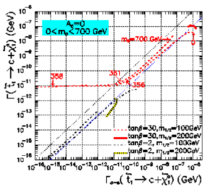
Figure 5.14: Comparison between the exact numerical calculation (ordinate) and the one–step approximation (abscissa) for the $\tilde{t}_{1}\to c\,\tilde{\chi}_{1}^{0}$ decay width for various values of $\tan\beta$ and $m_{1/2}$ with $A_{0}=0$ and $m_{0}$ varying in the indicated range. The dotted left diagonal line would signify the equality between the estimates, while the right diagonal line would indicate one order of magnitude difference. Results of both estimates indicated in the lower right legend. More details are found in the text.

5.1.3 Two-Body Decays of the Lightest Stop: the SSSM case

In contrast to the case of an $L$ conserving supergravity theory (MSUGRA), in the $L$ violating through Superrenormalizable terms (SSUGRA) case, one can have a competing $L$ violating stop decay mode in region I of Fig. 5.13. From eq. (4.2) with $\tau=F_{3}^{+}$ one can easily compute the $L$ violating stop decay width $\tilde{t}_{1}\to b\,\tau$,

$$\Gamma(\tilde{t}_{1}\to b\,\tau) = \frac{g^{2}\lambda^{1/2}(m_{\tilde{t}_{1}}^{2},m_{b}^{2},m_{\tau}^{2})}{16\pi m_{\tilde{t}_{1}}^{3}}\{-4U_{32}^{*}\hat{h}_{b}c_{\theta_{\tilde{t}}}(V_{32}^{*}\hat{h}_{t}s_{\theta_{\tilde{t}}}-V_{31}^{*}c_{\theta_{\tilde{t}}})m_{b}m_{\tau}$$ (5.10)

$$+[(V_{32}^{*}\hat{h}_{t}s_{\theta_{\tilde{t}}}-V_{31}^{*}c_{\theta_{\tilde{t}}})^{2}+U_{32}^{*2}\hat{h}_{b}^{2}c^{2}_{\theta_{\tilde{t}}}](m_{\tilde{t}_{1}}^{2}-m_{b}^{2}-m_{\tau}^{2})\}$$

which coincides with the result found in Ref. [70]. In [107] it was shown that, except for $U_{32}$ which determines the SU(2)-conserving mixing of the Higgsino with the left-handed $\tau$, all other mixing matrix elements $V_{3i}$ and $U_{3i}$ are proportional to $v_{3}^{II}$ (defined in eq. (1.14) )and therefore to the $\nu_{3}$ mass. Neglecting these terms we have from eq. (5.10)

$$\Gamma(\tilde{t}_{1}\to b\,\tau)\approx\frac{g^{2}\lambda^{1/2}(m_{\tilde{t}_{1}}^{2},m_{b}^{2},m_{\tau}^{2})}{16\pi m_{\tilde{t}_{1}}^{3}}\sin^{2}\xi^{\prime}\hat{h}_{b}^{2}c^{2}_{\theta_{\tilde{t}}}(m_{\tilde{t}_{1}}^{2}-m_{b}^{2}-m_{\tau}^{2})$$ (5.11)

noting that, to a good approximation,

$$|U_{32}|\approx\left|\frac{\mu_{3}}{\mu}\right|=|\sin\xi^{\prime}|$$ (5.12)

where $\mu_{3}$ corresponds to the superrenormalizable parameter in basis I defined in section 1.2. The lesson here is that the $L$ violating decay rate $\Gamma(\tilde{t}_{1}\to b\,\tau)$ is proportional to $\mu_{3}$ or, equivalently, to $\sin^{2}\xi^{\prime}$, instead of $\sin^{2}\xi$, and thus not necessarily small, since it is not directly controlled by the neutrino mass. In other words, there can be cancellations in the latter but not in the $L$ violating branching ratio.

The meaning of the factor $\sin^{2}\xi^{\prime}h_{b}^{2}$ may also be seen in basis II, where $\epsilon^{II}_{3}=0$. In this case $v_{3}^{II}$ is proportional to the $\nu_{3}$ mass so that, as already mentioned, in this basis all the elements $U_{3i}$ and $V_{3i}$ are small [92]. Neglecting these terms, $\Gamma(\tilde{t}_{1}\to b\,\tau)$ may be written directly from the interaction term $\tilde{t}_{L}b_{R}\tau_{L}$, which is induced by the trilinear term in the $\epsilon^{II}_{3}=0$–basis given in eq. (1.16) as

$$\lambda_{3}^{II}=\left(\mu_{3}/\mu\right)h_{b}=h_{b}\sin\xi^{\prime}$$ (5.13)

which is the factor in eq. (5.11). Note, however, that in our numerical calculation to be described below we have used for $\Gamma(\tilde{t}_{1}\to b\,\tau)$ the full expression given in eq. (4.1).

Next section we will determine the conditions under which the $L$ violating decay width $\Gamma(\tilde{t}_{1}\to b\,\tau)$ can be dominant over the $L$ conserving ones, $\Gamma(\tilde{t}_{1}\to c\,\tilde{\chi}_{1}^{0})$ and $\Gamma(\tilde{t}_{1}\to b\,\tilde{\chi}_{1}^{+})$.

Region I

Using the one-step approximation for $\Gamma(\tilde{t}_{1}\to c\,\tilde{\chi}_{1}^{0})$ one finds from eq. (5.2)

$$\Gamma(\tilde{t}_{1}\to c\,\tilde{\chi}_{1}^{0})\sim 10^{-6}h_{b}^{4}m_{\tilde{t}_{1}}\left(1-\frac{m_{\tilde{\chi}_{1}^{0}}^{2}}{m_{\tilde{t}_{1}}^{2}}\right)^{2}$$ (5.14)

Using the eq. (5.11) and neglecting charm, tau and bottom masses we get

$$\frac{\Gamma(\tilde{t}_{1}\to c\,\tilde{\chi}_{1}^{0})}{\Gamma(\tilde{t}_{1}\to b\,\tau)}\sim 10^{-5}\frac{h_{b}^{2}}{\sin^{2}\xi^{\prime}}\left(1-\frac{m_{\tilde{\chi}_{1}^{0}}^{2}}{m_{\tilde{t}_{1}}^{2}}\right)^{2}$$ (5.15)

Therefore $\Gamma(\tilde{t}_{1}\to c\,\tilde{\chi}_{1}^{0})$ will start to compete with $\Gamma(\tilde{t}_{1}\to b\,\tau)$ from $\sin\xi^{\prime}\lesssim 5\times 10^{-3}$ ($10^{-4}$) for $\tan\beta$ large (small). In Fig. 5.16 we compare $BR({\tilde{t}}_{1}\to c\,{\tilde{\chi}_{1}^{0}})$ [calculated numerically from their exact formula in (4.1)] with $BR({\tilde{t}}_{1}\to b\,\tau)$ within the restricted region of the $m_{{\tilde{t}}_{1}}$–$m_{{\tilde{\chi}}_{1}^{0}}$ plane where only those two decay modes are open. We consider different $m_{\nu_{3}}$ values (these correspond to relatively small values of the $L$ violating parameters $|\mu_{3}|,|v_{3}|\lesssim 1$ GeV). We vary the SSSM parameters randomly obeying the condition $m_{\tilde{t}_{1}}<m_{\tilde{\chi}^{\pm}_{1}}+m_{b}$ and depict the corresponding region in light grey. The upper–left triangular region is defined by kinematics and corresponds to $m_{\tilde{t}_{1}}<m_{\tilde{\chi}^{0}_{1}}+m_{c}$, so that $BR(\tilde{t}_{1}\to b\,\tau)=100\>\%$. The lower–right grey corresponds to $m_{\tilde{t}_{1}}>m_{\tilde{\chi}^{0}_{1}}+m_{c}$ when the sampling is done over the region defined by eq. (5.1.2). One notices from Fig. 5.16 that in the central region the dominant stop decay mode is $\tilde{t}_{1}\to b\,\tau$ with branching ratio $BR(\tilde{t}_{1}\to b\,\tau)>0.9$. The dotted lines in the light grey region indicate maximum $\nu_{3}$ mass values obtained in the scan. In the calculation of the $\nu_{3}$ mass, we have allowed only up to one order of magnitude of cancellation between the two terms which contribute to $\sin\xi$. Therefore if the lightest stop only decays into the two modes considered here, the processes $\tilde{t}_{1}\to b\,\tau$, will be important even for the case of very light $\nu_{3}$ masses.

Figure 5.15: Regions where the ${\tilde{t}}_{1}\to b\,\tau$ decay branching ratio exceeds 90% in the $m_{{\tilde{t}}_{1}}$–$m_{{\tilde{\chi}}_{1}^{0}}$ plane for different $m_{\nu_{3}}$ values. The SSSM parameters are randomly varied as indicated in the text under the restriction $m_{\tilde{t}_{1}}<m_{\tilde{\chi}^{\pm}_{1}}+m_{b}$. The upper–left triangular region corresponds to $m_{\tilde{t}_{1}}<m_{\tilde{\chi}^{0}_{1}}+m_{c}$ so that only the $\tilde{t}_{1}\to b\,\tau$ decay channel is open. The lower–right unshaded region corresponds to $m_{\tilde{t}_{1}}>m_{\tilde{\chi}^{+}_{1}}+m_{b}$.

Figure 5.16: $BR(\tilde{t}_{1}\to b\,\tau)$ as function of the lighter stop mass for $\nu_{3}$ mass in the sub–eV range and two different values of $\tan\beta$ and $\mu_{3}/\mu_{0}$. This prediction is natural in the sense that we have allowed only up to one order of magnitude of cancellation between the two terms that contribute to $\sin\xi$.

We note however that we can use the limits obtained from leptoquark searches [191] in order to derive limits on the top-squark in the SSSM. In particular, if $BR({\tilde{t}}_{1}\to b\tau)=1$ stop masses less than 99 GeV are excluded at 95% of CL., under the assumption that the three–body decays of the stops are negligible. Therefore, the dark region in Fig. 5.16 would be ruled out. In ref. [192] we have determined the corresponding restrictions on the SUGRA parameter space.

The dependence on the $\nu_{3}$ mass may be seen in Fig. 5.16 where the role played by $\tan\beta$ is manifest. In this figure we have shown $BR(\tilde{t}_{1}\to b\,\tau)$ as function of the lighter stop mass for $\nu_{3}$ mass in the sub–eV range, indicated by the simplest oscillation interpretation of the Super-Kamiokande atmospheric neutrino data. We have obtained such $\nu_{3}$ mass values numerically, allowing only one decade of cancellation between the two terms that contribute to $\sin\xi$ in eq. (1.28). The degree of suppression for $\mu_{3}/\mu_{0}$ obtained numerically agrees very well with the expectations from the approximate formula for the minimal $\nu_{3}$ mass in eq. (1.31). In contrast with Ref. [70], in our case $BR({\tilde{t}}_{1}\to b\tau)$ decreases with $\tan\beta$. The reason for this difference is that here we take into account the fact that the mixing parameter $\Gamma_{UL13}$ obtained from the RGE depends on $h_{b}^{2}$ in eq. (5.2), while in ref. [70] was simply regarded as a phenomenological input parameter (called $\delta$ there).

The message from this subsection is that in our SSUGRA the $L$ violating decay mode $\tilde{t}_{1}\to b\,\tau$ can very easily dominate the $L$ conserving decay mode $\tilde{t}_{1}\to c\,\tilde{\chi}_{1}^{0}$, even for very small neutrino masses.

Region II

In region II the $L$ conserving decay mode $\tilde{t}_{1}\to b\tilde{\chi}^{+}_{1}$ is open (but not $\tilde{t}_{1}\to t\nu$), and competes with the $L$ violating mode $\tilde{t}_{1}\to b\,\tau$. Replacing the subindex 3 by 1 on the diagonalization matrices $U$ and $V$ in eq. (5.10) we get the corresponding expression for $\Gamma(\tilde{t}_{1}\to b\,\tilde{\chi}_{1}^{+})$. In order to get an approximate expression for the ratio of the two main decay rates in this region, we note that in SUGRA with universality at the unification scale, the lightest chargino is usually gaugino-like, implying that $V_{11}^{2}\sim 1$. In addition, the lightest stop is usually right-handed, hence $\sin^{2}\theta_{\tilde{t}}\gtrsim\cos^{2}\theta_{\tilde{t}}$. This way we find

$$\frac{\Gamma(\tau)}{\Gamma(\tilde{\chi}_{1}^{+})}\equiv\frac{\Gamma(\tilde{t}_{1}\to b\,\tau)}{\Gamma(\tilde{t}_{1}\to b\,\tilde{\chi}_{1}^{+})}\approx\frac{\sin^{2}\xi^{\prime}\hat{h}_{b}^{2}\cos^{2}{\theta_{\tilde{t}}}}{\left[(V_{11}^{*}\cos{\theta_{\tilde{t}}}-V_{12}^{*}\hat{h}_{t}\sin{\theta_{\tilde{t}}})^{2}+U_{12}^{*2}\hat{h}_{b}^{2}\cos^{2}{\theta_{\tilde{t}}}\right]}\,K$$ (5.16)

where $K$ is a kinematical factor depending on the lightest stop and chargino masses, and here we have defined $\hat{h}_{t,b}\equiv h_{t,b}/g$. The presence of the bottom quark Yukawa coupling indicates that large values of $\tan\beta$ are necessary to have large $L$ violating branching ratios in this region. In fact, we have checked numerically with the exact expressions that in Region II (RII) ${\Gamma(\tau)}/{\Gamma(\tilde{\chi}_{1}^{+})}\gtrsim 1$ only for large $\tan\beta$ as we will see in the next figures.

In Fig. 5.17 we show the regions in the $m_{\chi^{\pm}_{1}}-m_{\tilde{t}_{1}}$ plane where $BR(\tilde{t}_{1}\to b\,\tau)$ dominates over $BR(\tilde{t}_{1}\to b\widetilde{\chi}^{+}_{1})$. In the upper–left region the decay mode $\tilde{t}_{1}\to b\widetilde{\chi}^{+}_{1}$ is not allowed and corresponds to Region I. Below and to the right of this zone, and above and to the left of three rising lines, lies region RII where ${\Gamma(\tau)}/{\Gamma(\tilde{\chi}_{1}^{+})}>1$. The three lines correspond to $|\mu_{3}|<80$ GeV (dashed), $|\mu_{3}|<60$ GeV (dotted), and $|\mu_{3}|<40$ GeV (dot–dashed), respectively. The proximity to the upper-left zone indicates that the $L$ violating decay dominates only close to the threshold where there is a high kinematical suppression of the $L$ conserving one, through the factor $K$. Unlike the case of region I this requires large values of the $L$ violating parameters. Note, moreover, that if the stops have a small mixing ($\cos{\theta_{\tilde{t}}}\approx 0$), then ${\Gamma(\tau)}/{\Gamma(\tilde{\chi}_{1}^{+})}\ll 1$ in RII.

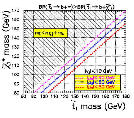
Figure 5.17: Contours of $BR({\tilde{t}}_{1}\to b\,\tau)>BR({\tilde{t}}_{1}\to b\tilde{\chi}_{1}^{+})$ in the $m_{{\tilde{t}}_{1}}$–$m_{{\tilde{\chi}}_{1}^{+}}$ plane for $|v_{3}|<10$ GeV. Three different maximum values for $|\mu_{3}|$ are considered: $|\mu_{3}|<40$ GeV (dot-dash), $|\mu_{3}|<60$ GeV (dots), and $|\mu_{3}|<80$ GeV (dashes). The region where $m_{\tilde{t}_{1}}<m_{b}+m_{\widetilde{\chi}^{+}_{1}}$ corresponds to the previously studied Region I.

A simpler expression for the ratio of decay rates in eq. (5.16) is obtained if we take $V_{11}\approx 1$ and assume no kinematical suppression in eq. (5.16) through the factor $K$:

$$\frac{\Gamma(\tau)}{\Gamma(\tilde{\chi}_{1}^{+})}\sim\sin^{2}\xi^{\prime}\hat{h}_{b}^{2}\,.$$ (5.17)

Note that the presence of the parameter $\sin\xi^{\prime}=\mu_{3}/\mu$ indicates that the $L$ violating decay mode is not strictly proportional to the neutrino mass, but proportional to the SSSM parameter $\mu_{3}^{2}$.

However generically we expect some correlation with the $\nu_{3}$ mass, especially in the case where the boundary conditions in the RGE are universal and there are no strong cancellations between two terms that contribute to $\sin\xi$ as shown in Fig. 5.19. In this figure we plot the ratio $\Gamma(\tau)/\Gamma(\tilde{\chi}_{1}^{+})$ in RII as a function of the $\nu_{3}$ mass. Both decay rates have been calculated numerically from the exact formulas. In this figure we have imposed both $m_{L_{0}}^{2}=M_{L}^{2}$ and $B_{0}=B_{3}$ within 0.1% at the GUT scale. Cancellation between the $\Delta m^{2}$ and $\Delta B$ terms in the neutrino mass formula of eq. (1.28) are accepted only within 1 decade. As a reference we have drawn the line corresponding to $\Delta B=0$ and $\Delta m^{2}=\Delta m^{2}_{min}$ ($\Delta m^{2}$ is negative and its magnitude is bounded from below by $\Delta m^{2}_{min}$) at the weak scale, which gives an idea of the value of the neutrino mass when there is no cancellation between the $\Delta B$ and $\Delta m^{2}$ terms.

We have imposed an upper bound on $m_{\nu_{3}}$ at the collider experimental limit of the $\nu_{3}$ mass, and have chosen fixed values of $\mu_{3}/\mu_{0}=1$, 0.1, and 0.01. The allowed region for $\mu_{3}/\mu_{0}=1$ is above the dashed line. In the case of $\mu_{3}/\mu_{0}=0.1$ (0.01) the allowed region lies enclosed between the solid (dotted) lines. The effect of $\tan\beta$ is to increase the ratio $\Gamma(\tau)/\Gamma(\tilde{\chi}_{1}^{+})$: the minimum value of the ratio is obtained for $\tan\beta\approx 2$ and the maximum corresponds to $\tan\beta\approx 60$. The extreme values of $\tan\beta$ are dictated by perturbativity.

Figure 5.18: Regions for $\Gamma({\tilde{t}}_{1}\to b\,\tau)/\Gamma({\tilde{t}}_{1}\to b\,{\tilde{\chi}_{1}^{+}})$ as a function of the $\nu_{3}$ mass with the universality condition $B_{0}=B_{3}$ at the unification scale imposed at the 0.1% level as indicated. Its effect is to alter the maximum attainable $\nu_{3}$ mass. The dot-dashed line corresponds to the case where $\Delta B=0$ at the weak scale.

Figure 5.19: Regions for $\Gamma({\tilde{t}}_{1}\to b\,\tau)/\Gamma({\tilde{t}}_{1}\to b\,{\tilde{\chi}_{1}^{+}})$ as a function of the $\nu_{3}$ mass for different levels of cancellation between the two terms that contribute to the neutrino mass. We impose the universality condition $m_{L_{0}}^{2}=M_{L}^{2}$ at the unification scale, but $B_{0}$ and $B_{3}$ are not universal. We take $|\mu_{3}/\mu_{0}|=1$ (inside the dashed lines), $|\mu_{3}/\mu_{0}|=0.1$ (solid lines), and $|\mu_{3}/\mu_{0}|=0.01$ (dotted lines).

A number of statistically less significant points appear outside the drawn regions in Fig. 5.19 and are not depicted. They correspond to points with $m_{\tilde{t}_{1}}-m_{b}-m_{{\tilde{\chi}}_{1}^{\pm}}<10\,$ GeV which appear above the diagonal line, and points with $\cos\theta_{\tilde{t}}<0.1$ which appear below the horizontal line corresponding to the lowest values of $\tan\beta$. In the last case, our approximation in eq. (5.17) does not work any more. On the other hand, eq. (5.17) predicts very well the behavior of $\Gamma(\tau)/\Gamma(\tilde{\chi}_{1}^{+})$ if $\cos\theta_{\tilde{t}}>0.1$. For example for $\mu_{3}/\mu_{0}=1$, or equivalently $\sin\xi^{\prime}=1/\sqrt{2}$, we expect from eq. (5.17) a maximum value of order 1 for large $\tan\beta$ ($h_{b}\approx 1$) and a minimum value of order $10^{-3}$ for small $\tan\beta$ ($h_{b}^{2}\approx 10^{-3}$), and this is confirmed by Fig. 5.19. High values of the $L$ violating branching ratio for large $\mu_{3}$ values are highly restricted for large $\tan\beta$. This can be understood as follows. In the case of $\mu_{3}/\mu_{0}=1$ and $\tan\beta=60$ acceptable neutrino masses are obtained only if $\sin\xi\sim 1$. On the other hand, in this regime we find from eq. (1.28) that the $\Delta B$ term is large because of the high value of $\tan\beta$, and that the $\Delta m^{2}$ term is large because $m_{L_{0}}^{2}$ becomes negative and $\Delta m^{2}=m_{L_{0}}^{2}-M_{L}^{2}$ grows in magnitude. This way, acceptable neutrino masses are achieved only with cancellation within more than one decade. In any case, we think that Fig. 5.19 is very conservative considering that in SSSM–SUGRA with unification of top-bottom-tau Yukawa couplings, the large value of $\tan\beta$ implies that a cancellation of four decades among vev’s is needed.

The width of the band in Fig. 5.19 reflects the degree of correlation between the ratio $\Gamma({\tilde{t}}_{1}\to b\,\tau)/\Gamma({\tilde{t}}_{1}\to b\,{\tilde{\chi}_{1}^{+}})$ and the neutrino mass under the mentioned conditions. Note that one would have an indirect measurement of the neutrino mass if this ratio were determined independently. The band will open to the left if one allows a stronger cancellation between the terms in $\Delta B$ and $\Delta m^{2}$. On the other hand it will open to the right if the universality between $B_{0}$ and $B_{3}$ is relaxed. This is shown in Fig. 5.19 where we plot the ratio $\Gamma(\tau)/\Gamma(\tilde{\chi}_{1}^{+})$ in RII as a function of the $\nu_{3}$ mass, but without imposing universality between $B_{3}$ and $B_{0}$. If we accept cancellation within one decade between the $\Delta B$ and $\Delta m^{2}$ terms, then the allowed region is at the right and below the corresponding dashed tilted line. If a larger degree of cancellation is accepted, the left boundary of the allowed region moves to the left as indicated in the figure, enhancing the $L$ violating channel. In addition if we accept only a decade of cancellation between the two terms that contribute to the $\nu_{3}$ mass, then our approximate formula which predicts the minimum $\nu_{3}$ mass in eq. (1.31) works very well.

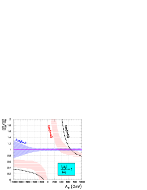
Figure 5.20: Universality condition $B_{0}=B_{3}$ at the unification scale as a function of $A_{0}$. As $\tan\beta$ increases, the allowed values of $A_{0}$ are more constrained.

In summary, in this subsection we have shown that even in region II, where the $L$ conserving decay mode ${\tilde{t}}_{1}\to b\,{\tilde{\chi}_{1}^{+}}$ is also open, the $L$ violating decay mode ${\tilde{t}}_{1}\to b\,\tau$ can be comparable to ${\tilde{t}}_{1}\to b\,{\tilde{\chi}_{1}^{+}}$ for large $\tan\beta$ and $\mu_{3}$, and relatively close to the chargino production threshold. In general, this implies a large neutrino mass unless a cancellation is accepted between the two terms contributing to the tree level neutrino mass. In addition, the non-universality of the $B_{0}$ and $B_{3}$ terms at the GUT scale does not increase appreciably the allowed parameter space, except at large $\tan\beta$. The main consequence of this non-universality is to restrict the allowed values of $A_{0}$ at large $\tan\beta$. In the next subsection we study the effects introduced by the non-universality of $m_{L_{0}}^{2}$ and $m_{L_{3}}^{2}$.

Effects of non–Universality

We now study the effect of possible non-universality of soft-breaking SUSY parameters on our previous results. In particular, the non-universality between $m_{L_{0}}^{2}$ and $m_{L_{3}}^{2}$ at the GUT scale. The SUGRA model with universality at the unification scale, while highly predictive, rests upon a number of simplifying assumptions which do not necessarily hold in specific models due to the possible evolution of the physical parameters in the range from $M_{Planck}$ to $M_{\mathrm{GUT}}$. Specifically, there are several models in the literature with non-universal soft SUSY breaking mass parameters at high scales. A recent survey can be found in [193], where several models such as based on string theory, M-theory, and anomaly mediated supersymmetry are analyzed. For this reason we find interesting to explore here the effects of non-universal soft terms.

The SUGRA spectra are typically found for given values of $m_{1/2}$, $m_{0}$, $A_{0}$, $\tan\beta$ and Sgn($\mu_{0}$). In our case we have in addition $\sin\xi^{\prime}$ (or equivalently, $\mu_{3}$). The value of $v_{3}$ is determined by the previous parameters through the minimization conditions. In addition, a relation between $A_{0}$ and the ratio $B_{3}/B_{0}$ at the GUT scale (which indicates the degree of universality) emerges. This relation can be seen in Fig. 5.20 for $\mu_{3}/\mu_{0}=1$ and the values $\tan\beta=3$, 40, and 60, for $m_{L_{0}}^{2}=M_{L}^{2}$. The relation becomes more restrictive as $\tan\beta$ is increased, starting from $-1000<A_{0}<1000$ GeV allowed for $\tan\beta=3$, to a single $A_{0}$ value compatible with unification for $\tan\beta=60$.

Figure 5.21: Comparison between the ratio $m_{L_{0}}^{2}/M_{L}^{2}$ at the weak and the unification scales for $\tan\beta=3$. Universality at the unification scale, $m_{L_{0}}^{2}/M_{L}^{2}=1$, implies a maximum value for this ratio at the weak scale.

Figure 5.22: $(m_{L_{0}}^{2}/M_{L}^{2})$ evaluated at the weak scale as a function of $\tan\beta$. This ratio is always less than one and decreases with $\tan\beta$.

Another way to enhance the $L$ violating channel, enlarging the band toward the left in Fig. 5.19, is by relaxing the universality between $m_{L_{0}}^{2}$ and $M_{L}^{2}$ at the GUT scale. In Fig. 5.22 we plot the ratio $m_{L_{0}}^{2}/M_{L}^{2}$ at the weak scale as a function of the same ratio at the unification scale $M_{\mathrm{GUT}}$ for $\tan\beta=3$. The shaded region is allowed, implying a maximum value for the ratio $m_{L_{0}}^{2}/M_{L}^{2}$ at the weak scale for a given value of the ratio at the GUT scale. We see from Fig. 5.22 that a relaxation of universality of 0.5% or more is enough to make $(m_{L_{0}}^{2}/M_{L}^{2})_{weak}=1$ possible, meaning that smaller neutrino masses are attainable without having to rely on a cancellation between the $\Delta m^{2}$ and $\Delta B$ terms or small values of $\Gamma({\tilde{t}}_{1}\to b\tau)$.

However as we increase $\tan\beta$ the maximum value of $m_{L_{0}}^{2}/M_{L}^{2}$ decreases, and thus, the required non-universality between $m_{L_{0}}$ and $M_{L}$ at unification scale grows drastically. In Fig. 5.22 we show the ratio $m_{L_{0}}^{2}/M_{L}^{2}$ at the weak scale as a function of $\tan\beta$. We appreciate clearly the growing of $|\Delta m^{2}|_{min}$ with $\tan\beta$. We remind the reader that this kind of non–universality in the soft terms is not uncommon in string models [194], or GUT models based on $SU(5)$ [195] or $SO(10)$ [196] for example. There are in fact some $SO(10)$ models for non-universality of the GUT scale scalar masses which naturally favor light neutrino mass [196].

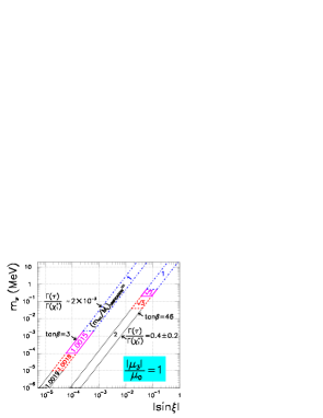
Figure 5.23: Minimum value of the $\nu_{3}$ mass as a function of $\sin\xi$ for different values of $m_{L_{0}}/M_{L}$ at the GUT scale and two values of $\tan\beta$. The ratio $\mu_{3}/\mu_{0}$ is fixed to the indicated value, leading to a nearly constant value for $\Gamma({\tilde{t}}_{1}\to b\,\tau)/\Gamma({\tilde{t}}_{1}\to b\,{\tilde{\chi}_{1}^{+}})$. Here we assume that the two terms contributing to the $\nu_{3}$ mass cancel to within an order of magnitude.

The effect of non–universality it is also explored in Fig. 5.23 where it is shown the relation between the neutrino mass and the parameter $\sin\xi$ for $\mu_{3}/\mu_{0}=1$. Two different bands are shown: one for $\tan\beta=3$ and $\Gamma(\tau)/\Gamma(\tilde{\chi}_{1}^{+})=2\times 10^{-3}$, and a second one for $\tan\beta=46$ and $\Gamma(\tau)/\Gamma(\tilde{\chi}_{1}^{+})=0.4\pm 0.2$. The required degree of universality at the GUT scale is indicated inside the bands. For example, in order to have neutrino masses of the order of eV for $\tan\beta=3$, $m_{L_{0}}^{2}$ needs to be at least 0.2% larger than $M_{L}^{2}$. Similarly, for $\tan\beta=46$ we need a $m_{L_{0}}^{2}$ twice as large as $M_{L}^{2}$ at the GUT scale in order to have neutrino masses of 1 eV. We stress the fact that for Fig. 5.23 we have conservatively accepted cancellation at the level of one order-of-magnitude only.

In summary, the lesson to learn here is that non-universal soft SUSY breaking terms at the GUT scale have the potential of making it easier to reconcile sizeable $L$ violating effects in the stop sector with very small neutrino masses, without resorting to cancellations.

5.2 Three Body Decays of stop

We discuss the phenomenology of the lightest stop in the SSSM. In this class of models we consider scenarios where the $L$ violating two-body decay ${\tilde{t}}_{1}\to\tau^{+}\,b$ competes with the leading three-body decays such as ${\tilde{t}}_{1}\to W^{+}\,b\,{\tilde{\chi}}^{0}_{1}$. We demonstrate that the $L$ violating decay can be sizable and in some parts of the parameter space even the dominant one. Moreover we discuss the expectations for ${\tilde{t}}_{1}\to\mu^{+}\,b$ and ${\tilde{t}}_{1}\to e^{+}\,b$. The recent results from solar and atmospheric neutrinos suggest that these are as important as the $\tau^{+}b$ mode. The ${\tilde{t}}_{1}\to l^{+}\,b$ decays are of particular interest for hadron colliders, as they may allow a full mass reconstruction of the lighter stop. Moreover these decay modes allow cross checks on the neutrino mixing angle involved in the solar neutrino puzzle complementary to those possible using neutralino decays [167]. For the so–called small mixing angle or SMA solution ${\tilde{t}}_{1}\to e^{+}\,b$ should be negligible, while for the large mixing angle type solutions all ${\tilde{t}}_{1}\to l^{+}\,b$ decays should have comparable magnitude. We first explore the extent to which the decay $\tilde{t}_{1}\to b\,\tau$ can be sizeable when compared with the 3–body decay modes. Moreover, we discuss the connections between the decay modes ${\tilde{t}}_{1}\to b\,l^{+}$ and neutrino physics, in particular we discuss a possible test of the solution to the solar neutrino puzzle. The appendixes in [106] contain complete formulas for the total widths of the three-body decay modes as well as for the couplings.

Notice that in SSUGRA models [31] $m_{\nu_{3}}$ is calculable through the RGE evolution and one finds in this case cancellations up to two orders of magnitude for the combination $\Lambda_{3}=-\mu_{3}v_{0}+\mu_{0}v_{3}$. In general the smallness of $m_{\nu_{3}}$ requires relatively small $\mu_{3}$ as in ref. [50]. The remaining two neutrinos acquire mass radiatively. Rigorous quantitative results were given in the second paper in ref. [34]. Typically they are hierarchically lighter than the heaviest neutrino, whose mass arises at the tree-level. This way one accounts for the observed hierarchy between the solar and the atmospheric neutrino mass scales.

In this section we present our numerical results for the branching ratios of the lighter stop $\tilde{t}_{1}$. Here we consider scenarios where all two-body decays induced at tree-level are kinematically forbidden except the $b\,l^{+}$ decays. Before going into detail it is useful to have some approximate formulas at hand [31]:

$$\Gamma(\tilde{t}_{1}\to b\,\tau)\approx\, \frac{g^{2}|U_{32}|^{2}h_{b}^{2}\cos^{2}_{\theta_{\tilde{t}}}m_{\tilde{t}_{1}}}{16\pi}\approx\frac{g^{2}|\mu_{3}|^{2}h_{b}^{2}\cos^{2}_{\theta_{\tilde{t}}}m_{\tilde{t}_{1}}}{16\pi|\mu_{0}|^{2}}$$ (5.18)

$$\Gamma(\tilde{t}_{1}\to c\tilde{\chi}_{1}^{0})\approx\, Fh_{b}^{4}(\delta_{m_{0}^{2}}\cos\theta_{\tilde{t}}-\delta_{A}\sin\theta_{\tilde{t}})^{2}f_{L}^{2}m_{\tilde{t}_{1}}\left(1-\frac{m_{\tilde{\chi}_{1}^{0}}^{2}}{m_{\tilde{t}_{1}}^{2}}\right)^{2}\,,$$ (5.19)

where $F=\frac{g^{2}}{16\pi}\left(\log(m_{\mathrm{GUT}}/m_{Z})K_{cb}K_{tb}/16\pi^{2}\right)^{2}\sim 6\times 10^{-7}$, $f_{L}=\sqrt{2}(\tan\theta_{W}\,N_{11}+3N_{12})/6$ and the parameter $\delta_{m_{0}^{2}}$ is given by

$$\delta_{m_{0}^{2}}=\frac{M_{Q}^{2}+M_{D}^{2}+m_{L_{0}}^{2}+A_{b}^{2}}{m_{\tilde{c}_{L}}^{2}-m_{\tilde{t}_{L}}^{2}}$$

For the minimal SUGRA models one finds $\delta_{m_{0}^{2}}={\cal O}(1)$ which is basically independent of the initial conditions due to the $m_{0}$ dependence both in the numerator and in the denominator. Finally we have

$$\delta_{A}=\frac{m_{t}(A_{b}+\frac{1}{2}A_{t})}{m_{\tilde{c}_{L}}^{2}-m_{\tilde{t}_{L}}^{2}}$$

The complete formulas are given in [31, 70], while for the three–body decays they are given in Section 4.2.2 . They reduce to the ones given in [73, 74] for vanishing $L$ violating parameters.

We have fixed the parameters as in [73] to avoid color breaking minima, while in the top squark sector we have used $m_{\tilde{t}_{1}}$, $\cos\theta_{\tilde{t}}$, $\tan\beta$, and $\mu_{0}$ as input parameters. For the sbottom sector we have fixed $M_{\tilde{Q}},M_{\tilde{D}}$ and $A_{b}$ as input parameters whereas for the charged scalars we took $m_{P^{0}_{2}}$, $M_{\widetilde{E}},M_{\tilde{L}}$, and $A_{\tau}$ as input . In addition we have chosen the $L$ violating parameters $\mu_{3}$ and $v_{3}$ in such a way that the heaviest neutrino mass is fixed with the help of eq. (1.26). For simplicity, we have also assumed that the soft SUSY breaking parameters are equal for all generations.

In order to get a feeling for minimal size of branching ratios that can be measured let us first shortly discuss the expected size for the direct production of light stops at future colliders. One expects for example at the LHC a production cross section of $\sim 35$ pb for 220 GeV stop mass. Therefore, once the full luminosity has been reached, one has to expect approximately 3.5 $10^{6}$ events per year. The corresponding stop production cross section at a future $e^{+}e^{-}$ linear collider of $800$ c.m.s. energy is of ${\cal O}(10-100\mathrm{fb})$ [78]. For an integrated luminosity of 500 fb^-1 per year one can expect ${\cal O}(10^{4})$ stop pairs per year. This implies that branching ratio as low as $10^{-3}$ can in principle be measured.

We consider first the simplest case of one generation model which, as already mentioned, is sufficient to describe the relative importance of the ${\tilde{t}}_{1}\to\tau^{+}\,b$ decay mode relative to the possible 3-body decay modes

$${\tilde{t}}_{1} \to W^{+}\,b\,{\tilde{\chi}}^{0}_{1}$$

$${\tilde{t}}_{1} \to S^{+}_{k}\,b\,{\tilde{\chi}}^{0}_{1}$$

$${\tilde{t}}_{1} \to S^{+}_{k}\,b\,\nu_{3}$$

$${\tilde{t}}_{1} \to b\,S^{0}_{i}\,\tau^{+}\,,$$ (5.20)

$${\tilde{t}}_{1} \to b\,P^{0}_{j}\,\tau^{+}\,$$

$${\tilde{t}}_{1} \to b\,{\tilde{l}}^{+}_{i}\,\nu_{l}\,,$$

$${\tilde{t}}_{1} \to b\,{\tilde{\nu}}_{l}\,l^{+}\hskip 28.45274pt(l=e,\mu)\,.$$

In general the important final states are those that conserve $L$. For example, for the case of decays involving $S^{+}_{k}$ the most important are those in which the scalars will be mainly a stau. Due to the fact that the existing bounds on the MSSM sneutrinos are below 100 GeV there exists the possibility that the sneutrino has nearly the same mass as one of the Higgs boson. Similarly it could be that the charged MSSM boson has nearly the same mass as one of the staus. This implies large mixing effects even for small $L$ violating parameters [84, 85, 105]. We therefore have used the complete formulas for the 3-body decay modes which are presented in the Appendix of [106]. The latter include $L$ violating decays such as $\tilde{t}_{1}\to W^{+}b\nu_{3}$. In addition to the above mentioned decays there is also ${\tilde{t}}_{1}\to b\,Z^{0}\,\tau^{+}$. This decay mode is kinematically suppressed compared to ${\tilde{t}}_{1}\to b\,\tau^{+}$ and there is no possible enhancement due to a mixing with an $L$ conserving final state. Therefore it can be safely neglected.

In Fig. 5.24 we show the branching ratios for the $\tilde{t}_{1}$ as a function of $\cos\theta_{\tilde{t}}$ in different scenarios. In order to calculate the partial width for the decay $\tilde{t}_{1}\to c\tilde{\chi}_{1}^{0}$ we have taken the formula given in ref. [71]. According to the analysis performed in [31], where the full calculation was done in the SUGRA scenario with universality at the unification scale, the result obtained with the present approximation should be taken as one upper bound. This implies also that the shown branching ratio for $\tilde{t}_{1}\to b\tau^{+}$ can be viewed as a lower bound. The parameters and physical quantities used in Fig. 5.24 are given in Tab. 5.3. For the case of Fig. 5.24(a) we have fixed in addition the $L$ violating parameters such that $m_{\nu}\approx 1$ eV. With this choice of parameters $S^{0}_{1}$, $S^{0}_{3}$, $P^{0}_{3}$, and $S^{-}_{4}$ are mainly the MSSM Higgs-bosons whereas $S^{0}_{2}$, $P^{0}_{2}$, $S^{-}_{2}$, and $S^{-}_{3}$ are mainly the MSSM sleptons of the third generation. In the plot we show the various branching ratios of the lighter stop summing up those branching ratios for the decays into sleptons that give the same final state, for example:

$${\tilde{t}}_{1}\to b\,\nu_{e}\,{\tilde{e}}^{+}_{L}\,\to\,b\,e^{+}\,\nu_{e}\,{\tilde{\chi}}^{0}_{1}\;,\hskip 14.22636pt{\tilde{t}}_{1}\to b\,e^{+}\,{\tilde{\nu}}_{e}\,\to\,b\,e^{+}\,\nu_{e}\,{\tilde{\chi}}^{0}_{1}\,.$$

The branching ratios for decays into $\tilde{\mu}_{L}$ or $\tilde{\nu}_{\mu}$ are practically the same as those into $\tilde{e}_{L}$ or $\tilde{\nu}_{e}$. Note that the energy spectrum of the leptons in the final will be somewhat different depending on whether the scalar in the intermediate step is charged or neutral. This offers in principle the possibility of determining the branching ratios of the different decay chains even if the final state topology is common. Note, that states containing scalars or neutralinos will lead to additional jet and/or lepton multiplicities absent in the MSSM.

Figure 5.24: Branching ratios for the $\tilde{t}_{1}$ as a function of $\cos\theta_{\tilde{t}}$ for different scenarios. We have fixed in a) $m_{\nu_{3}}=1\,$eV, b) $m_{\nu_{3}}=1\,$eV, $M_{\tilde{E}}>225\,$GeV, $M_{\tilde{L}}>225\,$GeV, c) $m_{\nu_{3}}=0.06\,$eV, $M_{\tilde{E}}>225\,$GeV, $M_{\tilde{L}}>225\,$GeV, d) Branching ratios for the $\tilde{t}_{1}$ as a function of $\cos\theta_{\tilde{t}}$ for $\tan\beta=3$. $m_{\nu_{3}}=0.06\,$eV, $M_{\tilde{E}}>225\,$GeV, $M_{\tilde{L}}>225\,$GeV. All the other inputs are given in Table 5.3.

In Fig. 5.24(b) the slepton mass parameters are chosen such that decays into scalars are kinematically forbidden. Here we display the channels ${\tilde{t}}_{1}\to b\,W^{+}{\tilde{\chi}}^{0}_{1}$, ${\tilde{t}}_{1}\to b\,\tau^{+}$ and ${\tilde{t}}_{1}\to c\,{\tilde{\chi}}^{0}_{1}$. The remaining modes, such as ${\tilde{t}}_{1}\to b\,S^{0}_{1}\,\tau^{+}$, turn out to be completely negligible. In both cases, with and without sleptons in the final state, one can see that in general the three body mode ${\tilde{t}}_{1}\to b\,W^{+}{\tilde{\chi}}^{0}_{1}$, dominates except for a somewhat narrow range of negative $\cos\theta_{\tilde{t}}$. However, the branching ratio for $\tilde{t}_{1}\to b\,\tau^{+}$ is above 0.1% for most values of $|\cos\theta_{\tilde{t}}|$ implying the observability of this mode. Most importantly, note that even in the parameter ranges where the three-body decay mode is dominant, its resulting signature is rather different from that of the MSSM due to the fact the lightest neutralino decays into SM-fermions, leading to enhanced jet and/or lepton multiplicities, as discussed in detail in [103, 167]. In the remaining part of this section we assume that 3-body decays into scalars are kinematically forbidden.

Input:	$\tan\beta=6$	$\mu_{0}=500$ GeV	$M_{2}=250$ GeV
	$M_{\tilde{D}}=370$ GeV	$M_{\tilde{Q}}=340$ GeV	$A_{b}=150$ GeV
	$M_{\tilde{E}}=210$ GeV	$M_{\tilde{L}}=210$ GeV	$A_{\tau}=150$ GeV
	$m_{{\tilde{t}}_{1}}=220$ GeV	$\cos\theta_{\tilde{t}}=-0.8$	$m_{P^{0}_{3}}=300$ GeV
Calculated	$m_{{\tilde{\chi}}^{0}_{1}}=122$ GeV	$m_{{\tilde{\chi}}^{+}_{1}}=234$ GeV	$m_{{\tilde{\chi}}^{+}_{2}}=519$ GeV
	$m_{{\tilde{b}}_{1}}=334$ GeV	$m_{{\tilde{b}}_{2}}=381$ GeV	$\cos\theta_{\tilde{b}}=0.879$
	$m_{S^{0}_{1}}=107$ GeV	$m_{S^{0}_{2}}=200$ GeV	$m_{S^{0}_{3}}=302$ GeV
	$m_{P^{0}_{2}}=200$ GeV	$m_{P^{0}_{3}}=300$ GeV
	$m_{S^{-}_{2}}=203$ GeV	$m_{S^{-}_{3}}=226$ GeV	$m_{S^{-}_{4}}=311$ GeV
	$m_{{\tilde{e}}_{L}}=215$ GeV	$m_{{\tilde{\nu}}_{e}}=m_{{\tilde{\nu}}_{\mu}}=200$ GeV

Table 5.3: Input parameters and resulting quantities used in Fig.  5.24.

In Fig. 5.24(c) the $L$ violating parameters are fixed in such a way that the heaviest neutrino mass is in the range suggested by the oscillation interpretation of the atmospheric neutrino anomaly [26].

Figure 5.25: Branching ratios for ${\tilde{t}}_{1}$ decays for $m_{{\tilde{t}}_{1}}=220$ GeV, $\mu_{0}=500$ GeV, $M_{2}=240$ GeV, and $m_{\nu}=100$, 1 and $0.06\,$eV. The branching ratios are shown as a function of $\tan\beta$. ($\cos\theta_{\tilde{t}}=-0.8$)

In Fig. 5.24(d) we show the same scenario as in Fig. 5.24(c) but for $\tan\beta=3$. The branching ratio into $b\tau$ now increases, whereas the branching ratio into $c\tilde{\chi}^{0}_{1}$ decreases. This is easily understood by inspecting eqs. (5.18) and (5.19). Indeed for the $b\,\tau$ case the partial width is proportional to $h_{b}^{2}$, whereas for $c\tilde{\chi}_{1}^{0}$ it is proportional to $h_{b}^{4}$. This implies that the partial width for $\tilde{t}_{1}\to c\tilde{\chi}_{1}^{0}$ grows faster with $\tan\beta$ than the width for $\tilde{t}_{1}\to b\,\tau$. This is also demonstrated in Fig. 5.25 where we show the $\tan\beta$ dependence of the branching ratio for the decay of $\tilde{t}_{1}$ into $b\tau^{+}$ for several values of the neutrino mass. For $m_{\nu_{3}}=0.06\,$eV the $BR(\tilde{t}_{1}\to b\,\tau)$ is still above $0.1\%$ if $\tan\beta$ is not too large, as favored by the explanation of the neutrino anomalies in this model [34]. As seen from the figure, the the $\tilde{t}_{1}\to b\tau^{+}$ branching ratio is also somewhat correlated to the $\nu_{3}$ mass. Should one add a sterile neutrino to the model [59], then the neutrino state $\nu_{3}$ could in principle be heavier than assumed above, favoring ${\tilde{t}}_{1}\to\tau^{+}\,b$ decay mode.

Let us now turn to the general three neutrinos case. There are new features that arise in this case, as opposed to the 1-generation case considered so far. In this model the solution to the present neutrino anomalies implies that all the $\mu_{i}$ are of the same order of magnitude [34].

Two further important results of [34] are that the atmospheric neutrino angle is controlled by the ratio $(-\mu_{2}v_{0}+\mu_{0}v_{2})/(-\mu_{3}v_{0}+\mu_{0}v_{3})$ and that the solar mixing angle is controlled by $(\mu_{1}/\mu_{2})^{2}$. One can get approximate formulas for the decay widths ${\tilde{t}}_{1}\to b\,e^{+}$ and ${\tilde{t}}_{1}\to b\,\mu^{+}$ similar to eq. (5.18) by replacing $\mu_{3}$ by $\mu_{1,2}$. This implies that (i) The decays into $b\,e^{+}$ and $b\,\mu^{+}$ are as important as the decay into $b\,\tau^{+}$. (ii) The decays ${\tilde{t}}_{1}\to b\,e^{+}$ and ${\tilde{t}}_{1}\to b\,\mu^{+}$ are related with the solar mixing angle. Moreover, we find that $\sum_{l=e,\mu,\tau}\Gamma(\tilde{t}_{1}\to b\,l^{+})$ in the 3-generation model is nearly equal to $\Gamma(\tilde{t}_{1}\to b\,\tau^{+})$ in the 1-generation model provided that $\sum_{i=1}^{3}\mu_{i}^{2}$ is identified to $\mu_{3}^{2}$ in the 1-generation model.

In Fig. 5.26 we show the ratio of $BR({\tilde{t}}_{1}\to b\,e^{+})/BR({\tilde{t}}_{1}\to b\,\mu^{+})$ versus $(\mu_{1}/\mu_{2})^{2}$ for different values of $\cos\theta_{\tilde{t}}$. For definiteness we have fixed the heaviest neutrino mass at the best-fit value indicated by the atmospheric neutrino anomaly. One can see that the dependence is nearly linear even for rather small $\cos\theta_{\tilde{t}}$. For $|\cos\theta_{\tilde{t}}|\lesssim 10^{-2}$ the approximation in eq. (5.18) breaks down and additional pieces dependent on $\sin\theta_{\tilde{t}}$ [31, 70] become important, leading to the non-linear dependence. One sees from the figure that, as long as $\cos\theta_{\tilde{t}}\gtrsim 10^{-2}$ there is a good degree of correlation between the branching ratios into $BR(\tilde{t}_{1}\to b\,e^{+})$ and $BR(\tilde{t}_{1}\to b\,\mu^{+})$ and the ratio $(\mu_{1}/\mu_{2})^{2}$. Thus by measuring these branchings one will get information on the solar neutrino mixing, since $\tan^{2}\theta_{sol}$ is proportional to $(\mu_{1}/\mu_{2})^{2}$ [34] which makes it a rather important quantity. For the so–called small mixing angle or SMA solution of the solar neutrino problem we expect ${\tilde{t}}_{1}\to e^{+}\,b$ to be negligible. In contrast, for the large mixing angle type solutions (LMA, LOW and QVAC, see ref. [26] and references therein) we expect all ${\tilde{t}}_{1}\to l^{+}\,b$ decays to have comparable rates. As a result in this model one can directly test the solution to the solar neutrino problem against the lighter stop decay pattern. This is also complementary to the case of neutralino decays considered in [167]. In that case the sensitivity is mainly to atmospheric mixing, as opposed to solar mixing. Testing the latter in neutralino decays at a collider experiment requires more detailed information on the complete spectrum to test the solar angle [167]. In contrast we have obtained here a rather neat connection of stop decays with the solar neutrino physics.

Figure 5.26: Ratio of branching ratios: $BR({\tilde{t}}_{1}\to be^{+})/BR({\tilde{t}}_{1}\to b\mu^{+})$ as a function of $(\mu_{1}/\mu_{2})^{2}$ for $m_{{\tilde{t}}_{1}}=220$ GeV, $\mu_{0}=500$ GeV, $M_{2}=240$ GeV; $|\cos\theta_{\tilde{t}}|\geq 0.1,0.01,10^{-3}$, $m_{\nu_{3}}=0.6$ eV.

Note, that this result is much more general than the scenarios discussed in this work. It is of particular importance in scenarios where only the $L$ violating decays and the decay into $\tilde{\chi}^{0}_{1}\,c$ are present [31, 70]. Similarly, the other ratios of the final states $b\,l^{+}$ are proportional to the square of the ratio of corresponding $\mu_{i}$ provided that $\cos\theta_{\tilde{t}}$ is not too small.

Chapter 6 Conclusions

We have seen in this work that the SSSM is a well motived model which also provides a solid explanation of the neutrino anomalies [34, 38] which can be tested at accelerators experiments. It reproduces the same signals that general $B_{p}$–SSM but with a minimum set of $L$ violating terms and automatically satisfies all the experimental bounds on induced dimension–4 $L$ violating operators. We have explicitly studied the phenomenology of neutralino and stop decays.

Concerning the Neutralinos, we have studied the production of the lightest neutralino $\tilde{\chi}^{0}_{1}$ at LEP2 and the resulting phenomenology in models where an effective superrenormalizable term parameterizes the explicit breaking of $L$. We have considered supergravity scenarios which can be explored at LEP2 in which the lightest neutralino is also the lightest supersymmetric particle. We have presented a detailed study of the LSP $\tilde{\chi}^{0}_{1}$ decay properties and studied the general features of the corresponding signals expected at LEP2. A detailed investigation of the possible detectability of the signals discussed in Tab. 5.1 taking into account realistic detector features is beyond the scope of this thesis. Clearly, existing LEP2 data are already probing the part of the parameter region which corresponds to approximately $m_{\tilde{\chi}^{0}_{1}}\lesssim 40$ GeV. Finally, we note that, in addition to important modifications in the $\tilde{\chi}^{0}_{1}$ decay properties, the SSSM lead also to new interesting features in other decays, such as charged [85] and neutral [84] Higgs boson and slepton decays, stop decays [31, 70], and gluino cascade decays [77, 197]. In addition we have shown that the SSSM can not be confused with gauge mediated supersymmetry breaking and conserved R-parity due to the absence of several final states in the GMSB case.

Concerning the stops we have studied the two–body decays of the lightest top squark in SUGRA models with and without $L$ violating terms. We have improved the calculation for the decay $\tilde{t}_{1}\to c\,\tilde{\chi}^{0}$ by numerically solving the renormalization group equations (RGE’s) of the SSSM including full generation mixing in the RGE’s for Yukawa couplings as well as soft SUSY breaking parameters. The decay-width is in general one order of magnitude smaller than the one obtained in the usual one–step approximation. This result will therefore enlarge the regions of parameter space where the four–body decays of lightest stop dominate over the decay into a charm quark and the lightest neutralino. As a result it will affect the present experimental lower bound on the $\tilde{t}_{1}$ mass even in the $L$ conserving case [76]. In the SSSM of course new decay modes appear and, as we have shown, they can be sizeable. In fact we have shown that the lightest stop can be the LSP, decaying with 100% rate into a bottom quark and a tau lepton. We have shown that the decay mode $\tilde{t}_{1}\to b\,\tau$ dominates over $\tilde{t}_{1}\to c\,\tilde{\chi}^{0}$ even for neutrino masses in the range suggested by the simplest oscillation interpretation of the Super-Kamiokande atmospheric neutrino data. This result would have a strong impact on the top squark search strategies at LEP [198] and TEVATRON [199], where it is usually assumed that the $\tilde{t}_{1}\to c\,\tilde{\chi}^{0}$ decay mode is the main channel. In addition to the signal of two jets and two taus present when the two produced stops decays through the $L$ violating channel, one expects a plethora of exotic high–multiplicity fermion events arising from neutralino decay, since such decay can happen inside the detector even for the small neutrino masses in the range suggested by the $\nu_{\mu}$ to $\nu_{\tau}$ oscillation interpretation of the atmospheric neutrino anomaly [34].

In addition the $L$ violating decay ${\tilde{t}}_{1}\to b\,\tau^{+}$ may compete with three–body decays. Specifically, we have found that for $m_{{\tilde{t}}_{1}}\lesssim 250$ GeV there are regions of parameter where ${\tilde{t}}_{1}\to b\,\tau^{+}$ is an important decay mode if not the most important one. This implies that there exists the possibility of full stop mass reconstruction from $\tau^{+}\,\tau^{-}\,b\,\bar{b}$ final states, favoring the prospects for its discovery. In contrast, in the MSSM the discovery of the lightest stop might not be possible at the LHC within this mass range. This implies that it is important to take into account this new decay mode when designing the stop search strategies at a future $e^{+}e^{-}$ Linear Collider. The SSSM also imply additional leptons and/or jets in stop cascade decays. Looking at the three generation model the decays into ${\tilde{t}}_{1}\to b\,l^{+}$ imply the possibility of probing $\mu^{2}_{1}/\mu^{2}_{2}$ and thus the solar mixing angle. This complements information which can be obtained using neutralino decays. In the latter case the sensitivity is mainly to the atmospheric mixing, as opposed to solar mixing [167]. In SSSM neutralino decays is ideal to test the atmospheric anomaly at a collider experiment, while stop decays provide neat complementary information on the solar mixing angle. Obtaining solar mixing information from neutralino decays would require more detailed knowledge on the supersymmetric spectrum, since it would be involved in the relevant loop calculations of the solar neutrino mass scale and mixing angle. By combining the two one can probe the parameters associated with both solar and atmospheric neutrino anomalies at collider experiments.

Appendix A Constraints on horizontal charges

In this Appendix we derive the general expressions for the individual field charges satisfying the set of 13 phenomenological and theoretical constraints corresponding to the six mass ratios for the quarks and the charged leptons plus the two quark mixing angles summarized in Table 2.3; the two relations provided by the absolute value of the masses of the third generation fermions; one phenomenological assumption about the charge of the $\mu_{0}$ term (2.20); one theoretical constraint corresponding to the consistency conditions for the coefficients of the mixed linear anomalies and one additional constraint from the vanishing of the mixed anomaly quadratic in the horizontal charges. As discussed in section 2.3.1, this leaves us with four free parameters that we choose to be $n_{i}$ ($i=1,2,3$) and $x$. We obtain

$$Q_{3} = \frac{1}{15\,\left(7+x\right)}\Big{[}-180-45x-3x^{2}+Q_{13}(41+5x)-7L_{23}+L_{23}^{2}$$

$$\hskip 42.67912pt+n_{1}(2+x+L_{23})+n_{2}(9+x-L_{23})+n_{3}(9+x)\Big{]},$$

$$L_{3} = \frac{1}{15\left(7+x\right)}\Big{[}20+50x+6x^{2}+18Q_{13}-21L_{23}+3L_{23}^{2}$$

$$\hskip 42.67912pt-n_{1}(29+2x-3L_{23})-n_{2}(8+2x+3L_{23})+n_{3}(97+13x)\Big{]},$$

where $L_{23}=L_{23}+l_{23}$ and $Q_{13}$ parametrized the two different possibilities for the quark and lepton charge differences given in Tab. (2.3). In terms of $Q_{3}$ and $L_{3}$ and of our four free parameters we have

$$\begin{array}[]{lll}H_{u}&=&n_{3}-L_{3}\\ L_{0}&=&-1+H_{u}\end{array}\qquad\qquad\qquad\begin{array}[]{lll}u_{3}&=&-Q_{3}-H_{u}\\ d_{3}&=&-Q_{3}+x-L_{0}\\ l_{3}&=&-L_{3}+x-L_{0}\end{array}$$

and from these all the other individual charges can be straightforwardly determined from the charge differences in Tab. (2.3). The solution for the charges in model MQ1+ML1 for the preferred values $n_{1}=n_{2}=n_{3}=-8$ and $x=1$ is given in Table A.1. For the $n_{0}=0$ case and the same value for the neutrino mass which implies in this case $n_{i}=-6-x$, we present in Table A.2 the individual charges in in model MQ1+ML1 for $x=0$

$Q_{1}$	$Q_{2}$	$Q_{3}$	$u_{1}$	$u_{2}$	$u_{3}$	$d_{1}$	$d_{2}$	$d_{3}$	$L_{1}$	$L_{2}$	$L_{3}$	$l_{1}$	$l_{2}$	$l_{3}$	$H_{u}$	$L_{0}$
$\frac{161}{30}$	$\frac{131}{30}$	$\frac{71}{30}$	$\frac{103}{15}$	$\frac{58}{15}$	$\frac{28}{15}$	$-\frac{18}{5}$	$-\frac{23}{5}$	$-\frac{23}{5}$	$-\frac{113}{30}$	$-\frac{113}{30}$	$-\frac{113}{30}$	$\frac{98}{15}$	$\frac{53}{15}$	$\frac{23}{15}$	$-\frac{127}{30}$	$\frac{97}{30}$

Table A.1: The anomaly free set of charges of model MQ1+ML1 for $x=1$ and $n_{1}=n_{2}=n_{3}=-8$

$Q_{1}$	$Q_{2}$	$Q_{3}$	$u_{1}$	$u_{2}$	$u_{3}$	$d_{1}$	$d_{2}$	$d_{3}$	$L_{1}$	$L_{2}$	$L_{3}$	$l_{1}$	$l_{2}$	$l_{3}$	$H_{u}$	$L_{0}$
$\frac{23}{5}$	$\frac{18}{5}$	$\frac{8}{5}$	$\frac{28}{5}$	$\frac{13}{5}$	$\frac{3}{5}$	$-\frac{14}{5}$	$-\frac{19}{5}$	$-\frac{19}{5}$	$-\frac{19}{5}$	$-\frac{19}{5}$	$-\frac{19}{5}$	$\frac{28}{5}$	$\frac{18}{5}$	$\frac{8}{5}$	$-\frac{11}{5}$	$\frac{11}{5}$

Table A.2: The anomaly free set of charges of model MQ1+ML1 for $n_{0}=0$, $x=0$ and $n_{1}=n_{2}=n_{3}=-6$

Appendix B Complete formulas for 2 body decays

In this Appendix we derive the Feynman rules $F_{j}^{0}q_{i}\tilde{q}_{k}$ (involving a neutralino/tau-neutrino, a quark, and a squark) and $F_{j}^{\pm}q_{i}\tilde{q}^{\prime}_{k}$ (involving a chargino/tau, a quark, and a squark of different electric charge) in the case of three generations and $L$ violating in the third generation. This is a generalization of the Feynman rules contained in [200], which hold for the MSSM and for one generation of quarks and squarks.

B.1 An explicit calculation

Before the general case, we will calculate here $\tilde{t}_{1}\to\tilde{\chi}_{1}^{0}\,t$.

From eq. (1.4), the lagrangian in terms of the two body decays are

$$\mathcal{L}_{t\tilde{t}\tilde{\chi}_{1}^{0}}=\left\{\frac{1}{\sqrt{2}}\tilde{t}_{L}^{*}\left[g(i\lambda^{3})t_{L}+g^{\prime}h_{t}(i\lambda^{\prime})t_{L}+\mathrm{h.c}\right]+\frac{1}{\sqrt{2}}g^{\prime}h_{t}\left[(i\lambda^{\prime})t_{L}\tilde{t}_{L}^{*}+\bar{t}_{L}(-i\bar{\lambda^{\prime}})\tilde{t}_{L}\right]\right.\\ -h_{t}\left.\left(\tilde{t}_{R}^{*}t_{L}\widetilde{H}_{u}^{0}+\widetilde{t}_{L}\bar{t}_{R}\widetilde{H}_{u}^{0}\right)\right\}$$ (B.1)

In terms of the four component spinors

$$\widetilde{B}=\begin{bmatrix}-i\lambda^{\prime}\\ i\bar{\lambda}^{\prime}\end{bmatrix},\qquad\widetilde{W}_{3}=\begin{bmatrix}-i\lambda^{3}\\ i\bar{\lambda}^{3}\end{bmatrix},\qquad\widetilde{H}_{u}=\begin{bmatrix}\widetilde{H}_{u}^{0}\\ \bar{\widetilde{H}}_{u}^{0}\end{bmatrix}$$ (B.2)

we have

$$\mathcal{L}_{t\tilde{t}\tilde{\chi}_{1}^{0}}=-\frac{1}{\sqrt{2}}\,\tilde{t}_{L}^{*}\left[g\overline{\widetilde{W}}_{3}P_{L}t+g^{\prime}h_{t}\overline{\widetilde{B}}P_{L}t\right]-\frac{1}{\sqrt{2}}\,g^{\prime}\left[h_{t}\bar{t}P_{L}\widetilde{B}\tilde{t}_{R}+h_{t}^{*}\overline{\widetilde{B}}P_{R}t\tilde{t}_{R}^{*}\right]\\ -\frac{g\,m_{t}}{\sqrt{2}m_{W}\sin\beta}\,\left[\overline{\widetilde{H}}_{u}P_{L}t\tilde{t}_{R}^{*}+\bar{t}P_{L}\widetilde{H}_{u}\tilde{t}_{L}\right]$$ (B.3)

The result in the mass basis is finally

$$\mathcal{L}_{t\tilde{t}\tilde{\chi}_{1}^{0}}=g\,\left\{\bar{t}\,\left[h^{t}_{ij}P_{L}+f^{t}_{1j}P_{R}\right]\tilde{\chi}_{j}^{0}\tilde{t}_{1}+\mathrm{h.c}\right\}$$ (B.4)

where

$$h^{t}_{1j}= \frac{m_{t}}{\sqrt{2}\,m_{W}\sin\beta}\,\left(\sin\beta{N^{\prime}_{j3}}^{*}-\cos\beta{N^{\prime}_{j4}}^{*}\right)\cos\theta_{\tilde{t}}$$

$$\quad+\left[\frac{-2\sqrt{2}}{3}\,\sin\theta_{W}\left(\tan\theta_{W}{N^{\prime}_{j2}}^{*}-{N^{\prime}_{j1}}^{*}\right)\right]\sin\theta_{\tilde{t}}$$ (B.5)

$$f^{t}_{1j}= \left[\frac{-2\sqrt{2}}{3}\,\sin\theta_{W}N^{\prime}_{j1}-\sqrt{2}\left(\frac{1}{2}-\frac{-2}{3}\sin\theta_{W}\right)\frac{N^{\prime}_{j2}}{\cos\theta_{W}}\right]\cos\theta_{\tilde{t}}$$

$$\quad+\left[\frac{m_{t}}{\sqrt{2}\,m_{W}\sin\beta}\left(\sin\beta N^{\prime}_{j3}-\cos\beta N_{j4}^{*}\right)\right]\sin\theta_{\tilde{t}}$$ (B.6)

where we have redefined the neutralino diagonalization matrix as

$$\begin{bmatrix}N^{\prime}_{j1}\\ N^{\prime}_{j2}\end{bmatrix}=\begin{bmatrix}\cos\theta_{W}&\sin\theta_{W}\\ -\sin\theta_{W}&\cos\theta_{W}\end{bmatrix}\begin{bmatrix}N_{j1}\\ N_{j2}\end{bmatrix},\qquad\begin{bmatrix}N^{\prime}_{j3}\\ N^{\prime}_{j4}\end{bmatrix}=\begin{bmatrix}\cos\beta&-\sin\beta\\ \sin\beta&\cos\beta\end{bmatrix}\begin{bmatrix}N_{j3}\\ N_{j4}\end{bmatrix}$$ (B.7)

We now calculate the two body width decay $\Gamma(\tilde{t}_{1}\to t+\tilde{\chi}_{1}^{0})$

$$\Gamma(\tilde{t}_{1}\to t+\tilde{\chi}_{1}^{0})=\frac{\Sigma_{S}|\mathcal{M}|^{2}}{16\pi\,m_{\tilde{t}_{1}}^{3}}\lambda^{3}(m_{\tilde{t}_{1}}^{2},m_{t}^{2},m_{\tilde{\chi}_{1}^{0}}^{2})$$ (B.8)

where $\lambda(a,b,c)=(a-b-c)^{2}-4ac$. The corresponding Feynman diagram is

$-ig[h^{t}_{ij}P_{L}+f^{t}_{1j}P_{R}]$

Consequently we can write down the amplitude as

$$\mathcal{M}=g\,\left[h^{t}_{1j}\,\bar{u}(p_{1})P_{L}v(p_{2})+f^{t}_{1j}\,\bar{u}(p_{1})P_{R}v(p_{2})\right]$$ (B.9)

The final result is

$$\Gamma(\tilde{t}_{1}\to t+\tilde{\chi}_{1}^{0})=\frac{g^{2}\lambda^{1/2}(m_{\tilde{t}_{1}}^{2},m_{t}^{2},m_{\tilde{\chi}_{1}^{0}}^{2})}{16\pi\,m_{\tilde{t}_{1}}^{3}}\left\{\left[(h^{t}_{1j})^{2}+(f^{t}_{1j})^{2}\right]\left(m_{\tilde{t}_{1}}^{2}-m_{t}^{2}-m_{\tilde{\chi}_{1}^{0}}^{2}\right)\right.\\ -\left.4h^{t}_{ij}f^{t}_{1j}m_{t}m_{\tilde{\chi}_{1}^{0}}\right\}$$ (B.10)

B.2 Couplings Neutralino–Squark-Quark

Following [201] we work in a quark interaction basis where $d_{L,R}=d_{L,R}^{0}$, $u_{L}=Ku_{L}^{0}$, and $u_{R}=u_{R}^{0}$ (we denote $q$ and $q^{0}$ the mass and current eigenstates respectively), as opposed to Ref. [202] where a more general basis is used. In addition, we implement the notation $\tilde{q}_{L,R}\equiv\tilde{q}^{0}_{L,R}$ for the interaction basis.

The starting point is the following piece of the Lagrangian

$${\cal L}_{u\tilde{u}F^{0}} = -g{\bar{u}}_{i}^{0}\Bigg{\{}\sqrt{2}\left[\sin\theta_{W}e_{U}{N^{\prime}}_{J1}+\frac{1}{\cos\theta_{W}}({\textstyle\frac{1}{2}}-e_{U}\sin^{2}\theta_{W}){N^{\prime}}_{J2}\right]\tilde{u}_{iL}$$ (B.11)

$$+\frac{m^{0U}_{ij}}{\sqrt{2}m_{W}\sin\beta\sin\theta}{N^{\prime}}_{J4}\tilde{u}_{jR}\Bigg{\}}P_{R}F_{J}^{0}$$

$$+g{\bar{u}}^{0}_{i}\Bigg{\{}\sqrt{2}\left[\sin\theta_{W}e_{U}{N^{\prime}}_{J1}^{*}+\frac{1}{\cos\theta_{W}}(-e_{U}\sin^{2}\theta_{W}){N^{\prime}}_{J2}^{*}\right]\tilde{u}_{iR}$$

$$-\frac{m^{0U\dagger}_{ij}}{\sqrt{2}m_{W}\sin\beta\sin\theta}{N^{\prime}}_{J4}^{*}\tilde{u}_{jL}\Bigg{\}}P_{L}F_{J}^{0}+\textrm{h.c.}$$

written in the quark interaction basis. The $5\times 5$ matrix $N^{\prime}$ diagonalizes the neutralino/neutrino mass matrix in the $(\tilde{\gamma},\tilde{Z},\tilde{L}_{0}^{0},\tilde{H}_{u}^{0},\nu_{\tau})$ basis as defined in [85], with the index $J=1...5$. The $3\times 3$ up–type quark mass matrix $m^{0U}$ is not diagonal, with the indexes $i,j=1,2,3$.

In order to write the above Lagrangian with mass eigenstates we use the basic relations mentioned before, in particular, $u_{iL}^{0}=(K^{\dagger})^{ij}u_{jL}$, which implies that ${\bar{u}}_{iL}^{0}={\bar{u}}_{jL}K^{ji}$. We need the following relations:

$$\begin{split}{\bar{u}}_{iL}^{0}\tilde{u}_{iL}=&{\bar{u}}_{iL}\left(\Gamma_{UL}^{*}{(K^{\dagger})}^{*}\right)^{ki}\tilde{u}_{k}\\ {\bar{u}}_{iL}^{0}m^{0U}_{ij}\tilde{u}_{jR}=&{\bar{u}}_{iL}(\Gamma_{UR}^{*}m^{U})^{ki}\tilde{u}_{k}\\ {\bar{u}}_{iR}\tilde{u}_{iR}=&{\bar{u}}_{iR}\Gamma_{UR}^{*ki}\tilde{u}_{k}\\ {\bar{u}}_{iR}m^{0U}_{ij}\tilde{u}_{jL}=&{\bar{u}}_{iR}(\Gamma_{UL}^{*}K^{*}{m}^{U})^{ki}\tilde{u}_{k}\end{split}$$ (B.12)

where $i,j=1,2,3$ label the quark flavors, $k=1...6$ labels the squarks, and $m^{U}\equiv{\mathrm{diag}}\,\{m_{u},m_{c},m_{t}\}$ is the diagonal up–type quark mass matrix. In this way, the Lagrangian in eq. (B.11) can be written as

$${\cal L}_{u\tilde{u}F^{0}}=-g{\bar{u}}_{i}[(\sqrt{2}G_{0UL}^{*jki}+H_{0UR}^{*jki})P_{R}-(\sqrt{2}G_{0UR}^{*jki}-H_{0UL}^{*jki})P_{L}]F_{j}^{0}\tilde{u}_{k}+\textrm{h.c.}$$ (B.13)

where the different couplings are

$$G_{0UL}^{jki} = \left[\sin\theta_{W}e_{U}{N^{\prime}}^{*}_{j1}+\frac{1}{\cos\theta_{W}}({\textstyle\frac{1}{2}}-e_{U}\sin^{2}\theta_{W}){N^{\prime}}^{*}_{j2}\right]\left(\Gamma_{UL}K^{\dagger}\right)^{ki}$$

$$G_{0UR}^{jki} = \left[\sin\theta_{W}e_{U}{N^{\prime}}_{j1}+\frac{1}{\cos\theta_{W}}(-e_{U}\sin^{2}\theta_{W}){N^{\prime}}_{j2}\right]\Gamma_{UR}^{ki}$$ (B.14)

$$H_{0UL}^{jki} = {N^{\prime}}_{j4}(\Gamma_{UL}K^{\dagger}{\hat{h}}_{U})^{ki}$$

$$H_{0UR}^{jki} = {N^{\prime}}^{*}_{j4}(\Gamma_{UR}\hat{h}_{U})^{ki}$$

and $\hat{h}_{U}\equiv$diag$\,(m_{u},m_{c},m_{t})/(\sqrt{2}m_{W}\sin\beta\sin\theta)$. Graphically, the $F_{j}^{0}u_{i}\tilde{u}_{k}$ Feynman rules are given by

$-ig[(\sqrt{2}G_{0UL}^{jki}+H_{0UR}^{jki})P_{L}-(\sqrt{2}G_{0UR}^{jki}-H_{0UL}^{jki})P_{R}]$

$-ig[(\sqrt{2}G_{0UL}^{*jki}+H_{0UR}^{*jki})P_{R}-(\sqrt{2}G_{0UR}^{*jki}-H_{0UL}^{*jki})P_{L}]$
The analogous Feynman rules in the MSSM are obtained by replacing $F_{i}^{0}\to\tilde{\chi}^{0}_{i}$, by interpreting the matrix $N$ as the usual $4\times 4$ neutralino mixing matrix, and by setting $\theta=\pi/2$ in the formula for the Yukawa couplings.

Similarly, replacing all $u(\tilde{u})$ by $d(\tilde{d})$ in eq. (B.11) and starting from

$$\begin{split}{\cal L}_{q\tilde{q}^{\prime}F^{+}}=&g\bar{d}_{i}\left[\frac{m^{0U\dagger}_{ij}}{\sqrt{2}m_{W}\sin\beta\sin\theta}V_{J2}\tilde{u}_{jR}-V_{J1}\tilde{u}_{iL}\right]P_{R}F^{c}_{J}\\ &+g\bar{d}_{i}\frac{m^{D}_{ij}}{\sqrt{2}m_{W}\cos\beta\sin\theta}U^{*}_{J2}\tilde{u}_{jL}P_{L}F^{c}_{J}\\ &+g\bar{u}^{0}_{i}\left[\frac{m^{D\dagger}_{ij}}{\sqrt{2}m_{W}\cos\beta\sin\theta}U_{J2}\tilde{d}_{jR}-U_{J1}\tilde{d}_{iL}\right]P_{R}F^{+}_{J}\\ &+g\bar{u}^{0}_{i}\frac{m^{0U}_{ij}}{\sqrt{2}m_{W}\cos\beta\sin\theta}V^{*}_{J2}\tilde{b}_{jL}P_{L}F^{+}_{J}+\hbox{h.c}\end{split}$$ (B.15)

we can obtain the complete Feynman rules for the neutralino/tau–neutrino and chargino/tau with quarks and squarks. The results, that complements the obtained in [201], are

Neutralino–(d)quark–(d)squark

$-ig[(\sqrt{2}G_{0DL}^{jki}+H_{0DR}^{jki})P_{L}-(\sqrt{2}G_{0DR}^{jki}-H_{0DL}^{jki})P_{R}]$

$-ig[(\sqrt{2}G_{0DL}^{*jki}+H_{0DR}^{*jki})P_{R}-(\sqrt{2}G_{0DR}^{*jki}-H_{0DL}^{*jki})P_{L}]$

The mixing matrices $G_{0D}$ and $H_{0D}$ are defined as

$$\begin{split}G_{0DL}^{jki}=&\left[\sin\theta_{W}e_{D}{N^{\prime}}_{j1}^{*}+\frac{1}{\cos\theta_{W}}(T_{3D}-e_{D}\sin^{2}\theta_{W}){N^{\prime}}^{*}_{j2}\right]\Gamma_{DL}^{ki}\\ G_{0DR}^{jki}=&\left[\sin\theta_{W}e_{D}{N^{\prime}}_{j1}+\frac{1}{\cos\theta_{W}}(-e_{D}\sin^{2}\theta_{W}){N^{\prime}}_{j2}\right]\Gamma_{DR}^{ki}\\ H_{0DL}^{jki}=&{N^{\prime}}_{j3}(\Gamma_{DL}{\hat{h}}_{D})^{ki}\\ H_{0DR}^{*jki}=&{N^{\prime}}_{j3}^{*}(\Gamma_{DR}\hat{h}_{D})^{ki}\end{split}$$ (B.16)

B.3 Couplings Chargino-Squark-Quark

Here we give the couplings that were used in Sections B.2 and 4.2.2

Chargino/tau–(d)quark–(u)squark

$-ig(-C^{-1})[(G_{UL}^{jki}-H_{UR}^{jki})P_{L}-H_{UL}^{jki}P_{R}]$

$-ig[(G_{UL}^{*jki}-H_{UR}^{*jki})P_{R}-H_{UL}^{*jki}P_{L}]C$

where $C$ is the charge conjugation matrix (in spinor space) and the mixing matrices $G_{U}$ and $H_{U}$ are defined as

$$\begin{split}G_{UL}^{jki}&\equiv V_{j1}^{*}\Gamma_{UL}^{ki},\qquad H_{UL}^{jki}\equiv U_{j2}^{*}(\Gamma_{UL}\hat{h}_{D})^{ki},\\ H_{UR}^{jki}&\equiv V_{j2}^{*}(\Gamma_{UR}\hat{h}_{U}K)^{ki},\end{split}$$ (B.17)

Chargino/tau–(u)quark–(d)squark

$-ig(-C^{-1})[(G_{DL}^{jki}-H_{DR}^{jki})P_{L}-H_{DL}^{jki}P_{R}]$

$-ig[(G_{DL}^{*jki}-H_{DR}^{*jki})P_{R}-H_{DL}^{*jki}P_{L}]C$

where the mixing matrices $G_{D}$ and $H_{D}$ are defined as

$$\begin{split}G_{DL}^{jki}\equiv&U_{j1}^{*}(\Gamma_{DL}K^{\dagger})^{ki},\qquad H_{DL}^{jki}\equiv V_{j2}^{*}(\Gamma_{DL}K^{\dagger}\hat{h}_{U})^{ki},\\ H_{DR}^{jki}\equiv&U_{j2}^{*}(\Gamma_{DR}\hat{h}_{D}K^{\dagger})^{ki},\end{split}$$ (B.18)

In order to derive the decays widths we write, for example eq. (B.13) as

$${\cal L}_{u\tilde{u}F^{0}}=g{\bar{u}}_{i}^{0}(f^{*jki}_{U}P_{R}+h^{*jki}_{U}P_{L})F_{j}^{0}\tilde{u}_{k}+\textrm{h.c}$$ (B.19)

The result is presented in Sec. 4.2.1.

Agradecimientos

Una ventaja de haber realizado el doctorado fuera de mi país es que ahora puedo agradecer a todas las personas que he conocido durante los cuatro años que más rápido han transcurrido en mi vida.

En primer lugar me gustaría agradecer la paciencia de mi familia para afrontar mis prolongadas ausencias sobre todo en la fase final de la escritura de este trabajo: mi esposa Tatiana, mi hija Sara y su abuela Margarita.

A José por su constante apoyo en lo académico y en lo personal. A los demás que hicieron posible esta Tesis: Andrew Akeroyd, Alfred Bartl, Alexander Belayev, Fernando de Campos, Marco A. Díaz, Oscar Eboli, Miguel Ángel García Jareño, Javier Ferrandis, Martín Hirsch, Mauricio Magro, Jesús Maria Mira, Enrico Nardi, William Ponce, Werner Porod, Diego Francisco Rodrigez, Jorge Crispim Romao y Emilio Torrente. Mis especiales agradecimientos al grupo de los Profesores Bartl y Majerotto en Viena, de Oscar Eboli en Brasil, y Enrico Nardi en Colombia por la cordial invitación, la amabilidad dispensada y el buen ambiente de trabajo generado en mis respectivas visitas a sus grupos. A mi familia en Colombia (mis padres y Wilson, Liliana, Mónica y Jorge) y, finalmente a COLCIENCIAS

A la amistad y/o ayuda de las personas relacionadas con el grupo durante este tiempo: Orlando, Sergio, Omar, Nicolao, Hiroshi, Nuria, Concha, Ricard, Verónica, Carlos, Isabel, Sabina, Florian, Cecilia, Victor, Kostas, Michele, Ara, Alexander Res, Timur, Maria Amparo, Thomas, $\ldots$.

A las personas que conocí a través de mi esposa y con quien departimos tantas veladas músico–gastronómicas. En especial a Ángeles y su familia por su innumerables atenciones, a Nuria a quien nucna olvidaré, a Virgilio (sus incontables ayudas informáticas) y su familia en Albacete, a Alejandro y su familia en Denia, a los de la casa de todos: Gerardo, Julio, Celine, Oscar (y los paseos al campo), Pilar. A Daniela, Ana, Amparo, Piñero, Marcos, Sonia, Maria Angeles, Tony y Rosana, Rubén, Carlos, Kico y Mónica, Manolo, $\ldots$

A los que pasaron por nuestra casa dejando huella: Ricardo, William, Enrico, Maria Fernanda, Jorge, Diego, Wilson, Sonia, Jesús Maria, Maria Eugenia, Sara Maria Mira Puerta, Inés Dalila, Orlando, Omar, Antonio y Parménides.

Finalmente a los que desarrollaron xemacs($+$AucTeX$+$ref$+$X-symbol$+$flyspell) por facilitarme de manera sustancial la escritura de éste trabajo.

Bibliography

• [1] 111Bash scripts to automatically produce a new  file with the $\backslash$cite’s and $\backslash$bibitem’s ordered, or to convert “$\backslash$def$\backslash$journal-name$\#$1$\#$2$\#$3...” citations into the spires format (wget is used for the automatic download), are available at http://ific.uv.es/$\sim$restrepo/autoeditlatex/ H. P. Nilles, Phys. Rept.  110 (1984) 1.
• [2] H. E. Haber and G. L. Kane, Phys. Rept.  117 (1985) 75.
• [3] X. Tata, hep-ph/9510287, Talk given at Theoretical Advanced Study Institute in Elementary Particle Physics (TASI 95): QCD and Beyond, Boulder, CO. In ”Boulder 1995, QCD and beyond” 163-219.
• [4] C. D. Carone, L. J. Hall and H. Murayama, Phys. Rev. D 54 (1996) 2328 [hep-ph/9602364].
• [5] G. R. Farrar and P. Fayet, Phys. Lett. B 76, 575 (1978).
• [6] S. Dimopoulos and H. Georgi, Nucl. Phys. B 193, 150 (1981).
• [7] L. E. Ibanez and G. G. Ross, Nucl. Phys. B 368, 3 (1992).
• [8] M. C. Bento, L. Hall and G. G. Ross, Nucl. Phys. B 292, 400 (1987).
• [9] L. E. Ibanez and G. G. Ross, Phys. Lett. B 260, 291 (1991).
• [10] L. E. Ibanez, Nucl. Phys. B 398, 301 (1993) [hep-ph/9210211].
• [11] I. Hinchliffe and T. Kaeding, Phys. Rev. D 47, 279 (1993).
• [12] G. Eyal and Y. Nir, JHEP 9906 (1999) 024 [hep-ph/9904473]. and ref 1-16 there
• [13] K. Choi, K. Hwang and E. J. Chun, Phys. Rev.  D 60 (1999) 031301 [hep-ph/9811363];
• [14] C. S. Aulakh and R. N. Mohapatra, Phys. Lett.  B 121 (1983) 147.
• [15] G. G. Ross and J. W. F. Valle, Phys. Lett.  B 151 (1985) 375;
• [16] L. J. Hall and M. Suzuki, Nucl. Phys.  B 231 (1984) 419.
• [17] J. Ellis, G. Gelmini, C. Jarlskog, G. G. Ross and J. W. F. Valle, Phys. Lett. B 150, 142 (1985)
• [18] I. Lee, Phys. Lett. B 138, 121 (1984). I. Lee, Nucl. Phys. B 246, 120 (1984).
• [19] S. Dawson, Nucl. Phys. B 261, 297 (1985).
• [20] M. J. Hayashi and A. Murayama, Phys. Lett. B 153, 251 (1985); R. N. Mohapatra, Phys. Rev. D 34, 3457 (1986); R. N. Mohapatra, Phys. Rev. Lett.  56, 561 (1986); H. Konig, Z. Phys. C 44, 401 (1989).
• [21] S. Dimopoulos and L. J. Hall, Phys. Lett.  B 207 (1988) 210;
• [22] A. Santamaria and J. W. Valle, Phys. Lett.  B 195 (1987) 423; Phys. Rev.  D 39 (1989) 1780; and Phys. Rev. Lett.  60 (1988) 397.
• [23] For a recent review see J. W. Valle, Proceedings of PASCOS98, ed. P. Nath, W. Scientific, hep-ph/9808292; J. W. Valle, lectures given at the VIII Jorge Andre Swieca Summer School (Rio de Janeiro, February 1995) and at V Taller Latinoamericano de Fenomenologia de las Interacciones Fundamentales (Puebla, Mexico, October 1995), hep-ph/9603307.
• [24] H. Dreiner, hep-ph/9707435.
• [25] R. Barbier et al., hep-ph/9810232.
• [26] M. C. Gonzalez-Garcia, M. Maltoni, C. Pena-Garay and J. W. F. Valle, Phys. Rev. D 63 (2001) 033005 [hep-ph/0009350] and references therein.
• [27] P. Abreu et al. [DELPHI Collaboration], Phys. Lett. B 502, 24 (2001) [hep-ex/0102045].
• [28] P. Abreu et al. [DELPHI Collaboration], Phys. Lett. B 502, 24 (2001).
• [29] P. Abreu et al. [DELPHI Collaboration], Phys. Lett. B 500, 22 (2001) [hep-ex/0103015]; D. Buskulic et al. [ALEPH Collaboration], Phys. Lett. B 384, 461 (1996); D. Buskulic et al. [ALEPH Collaboration], Phys. Lett. B 349, 238 (1995); J. F. Cavaignac, B. Vignon and R. Wilson, Phys. Lett. B 67, 148 (1977).
• [30] V. Barger, G. F. Giudice and T. Han, Phys. Rev. D 40, 2987 (1989).
• [31] M. A. Diaz, D. A. Restrepo and J. W. F. Valle, Nucl. Phys. B 583 (2000) 182 [hep-ph/9908286].
• [32] B. Allanach et al., “Searching for R-parity violation at Run-II of the Tevatron,” hep-ph/9906224.
• [33] A. Datta, B. Mukhopadhyaya and F. Vissani, Phys. Lett. B 492 (2000) 324 [hep-ph/9910296].
• [34] J. C. Romao, M. A. Diaz, M. Hirsch, W. Porod and J. W. Valle, Phys. Rev. D 61 (2000) 071703 [hep-ph/9907499]; M. Hirsch, M. A. Diaz, W. Porod, J. C. Romao and J. W. Valle, Phys. Rev. D 62 (2000) 113008 [hep-ph/0004115].
• [35] A. Belyaev, O.J.P. Eboli, W. Porod D.A. Restrepo, and J.W.F. Valle, work in progress
• [36] S. P. Martin, “A supersymmetry primer,”hep-ph/9709356;
• [37] A. Y. Smirnov and F. Vissani, Nucl. Phys. B 460, 37 (1996) [hep-ph/9506416].
• [38] R. Hempfling, Nucl. Phys. B 478 (1996) 3 [hep-ph/9511288].
• [39] K. Tamvakis, Phys. Lett. B 383 (1996) 307 [hep-ph/9602389].
• [40] K. Choi, E. J. Chun and H. Kim, Phys. Lett. B 394 (1997) 89 [hep-ph/9611293].
• [41] H. Nilles and N. Polonsky, Nucl. Phys. B 484 (1997) 33 [hep-ph/9606388].
• [42] K. Benakli and A. Y. Smirnov, Phys. Rev. Lett.  79 (1997) 4314 [hep-ph/9703465].
• [43] G. F. Giudice and R. Rattazzi, Phys. Lett. B 406 (1997) 321 [hep-ph/9704339].
• [44] P. Binetruy, E. Dudas, S. Lavignac and C. A. Savoy, Phys. Lett. B 422 (1998) 171 [hep-ph/9711517].
• [45] A. S. Joshipura and A. Y. Smirnov, Phys. Lett. B 439 (1998) 103 [hep-ph/9806376].
• [46] E. J. Chun and H. B. Kim, Phys. Rev. D 60 (1999) 095006 [hep-ph/9906392].
• [47] D. E. Kaplan and A. E. Nelson, JHEP 0001 (2000) 033 [arXiv:hep-ph/9901254].
• [48] J. L. Chkareuli, I. G. Gogoladze, A. B. Kobakhidze, M. G. Green and D. E. Hutchcroft, Phys. Rev. D 62 (2000) 015014 [hep-ph/9908451].
• [49] J. L. Chkareuli and C. D. Froggatt, Phys. Lett. B 484 (2000) 87 [hep-ph/0004090].
• [50] J. M. Mira, E. Nardi, D. A. Restrepo and J. W. Valle, Phys. Lett. B 492 (2000) 81 [hep-ph/0007266].
• [51] J. W. Valle, Phys. Lett. B 196 (1987) 157.
• [52] A. Masiero and J. W. Valle, Phys. Lett. B 251 (1990) 273;
• [53] J. C. Romao, C. A. Santos and J. W. Valle, Phys. Lett. B 288 (1992) 311; M. Chaichian and A. V. Smilga, Phys. Rev. Lett.  68 (1992) 1455; J. C. Romao, A. Ioannisian and J. W. Valle, Phys. Rev. D 55 (1997) 427 [hep-ph/9607401].
• [54] G. F. Giudice, A. Masiero, M. Pietroni and A. Riotto, Nucl. Phys. B 396 (1993) 243; [hep-ph/9209296]; M. Shiraishi, I. Umemura and K. Yamamoto, Phys. Lett. B 313 (1993) 89; see also I. Umemura and K. Yamamoto, Nucl. Phys. B 423 (1994) 405; K. Enqvist, K. Huitu and P. N. Pandita, Phys. Lett. B 366 (1996) 181 [hep-ph/9507227]; J. R. Espinosa, Phys. Lett. B 353 (1995) 243 [hep-ph/9503255].
• [55] M. Chaichian and R. Gonzalez Felipe, Phys. Rev. D 47 (1993) 4723.
• [56] R. Adhikari and B. Mukhopadhyaya, Phys. Lett. B 378 (1996) 342 [Erratum-ibid. B 384 (1996) 492] [hep-ph/9601382].
• [57] M. Frank and K. Huitu, hep-ph/0106004.
• [58] P. Nogueira, J. C. Romao and J. W. Valle, Phys. Lett. B 251 (1990) 142; J. C. Romao, J. Rosiek and J. W. Valle, Phys. Lett. B 351 (1995) 497 [hep-ph/9502211]; J. C. Romao, N. Rius and J. W. Valle, Nucl. Phys. B 363 (1991) 369.
• [59] M. Hirsch and J. W. F. Valle, Phys. Lett. B 495 (2000) 121 [hep-ph/0009066].
• [60] R. Barbieri, D. E. Brahm, L. J. Hall and S. D. Hsu, Phys. Lett. B 238 (1990) 86.
• [61] B. Mukhopadhyaya, S. Roy and F. Vissani, Phys. Lett. B 443 (1998) 191 [hep-ph/9808265].
• [62] L. Navarro, W. Porod and J. W. Valle, Phys. Lett. B 459 (1999) 615 [hep-ph/9903474].
• [63] T. Feng, Commun. Theor. Phys.  33 (2000) 421 [hep-ph/9806505]; hep-ph/9808379; C. Chang and T. Feng, Eur. Phys. J. C 12 (2000) 137 [hep-ph/9901260].
• [64] S. Y. Choi, E. J. Chun, S. K. Kang and J. S. Lee, Phys. Rev. D 60 (1999) 075002 [hep-ph/9903465].
• [65] The signals relevant for LEP2 are discussed e.g. in S. Ambrosanio and B. Mele, Phys. Rev.  D 52 (1995) 3900.
• [66] For a general review see of GMSB: G. F. Giudice and R. Rattazzi, Phys. Rept.  322 (1999) 419.
• [67] P. Abreu et al. [DELPHI Collaboration], CERN-EP-99-049; J.-F. Grivaz, Rapporteur Talk, International Europhysics Conference on High Energy Physics, Brussels, 1995; D. Buskulic et al. [ALEPH Collaboration], Phys. Lett. B 373 (1996) 246.
• [68] B. Abbott et al. [D0 Collaboration], Phys. Rev. Lett.  83 (1999) 4937 [hep-ex/9902013]; S. Abachi et al. [D0 Collaboration], Phys. Rev. Lett.  75 (1995) 618; F. Abe et al. [CDF Collaboration], Phys. Rev. Lett.  69 (1992) 3439; J. Alitti et al. [UA2 Collaboration], Phys. Lett. B 235 (1990) 363.
• [69] B. Abbott et al. [D0 Collaboration], Phys. Rev. D 62 (2000) 071701 [hep-ex/0005034].
• [70] A. Bartl, W. Porod, M. A. Garcia-Jareno, M. B. Magro, J. W. F. Valle and W. Majerotto, Phys. Lett. B 384 (1996) 151 [hep-ph/9606256].
• [71] K. Hikasa and M. Kobayashi, Phys. Rev. D 36 (1987) 724.
• [72] H. Baer, M. Drees, R. Godbole, J. F. Gunion and X. Tata, Phys. Rev. D 44 (1991) 725; T. Kon and T. Nonaka, hep-ph/9404230; T. Kon and T. Nonaka, Phys. Lett. B 319 (1993) 355 [hep-ph/9309286]; T. Kon, T. Kobayashi, S. Kitamura, K. Nakamura and S. Adachi, Z. Phys. C 61 (1994) 239 [hep-ph/9307312];
• [73] W. Porod, Phys. Rev.  D 59 (1999) 095009 [hep-ph/9812230].
• [74] W. Porod and T. Wohrmann, Phys. Rev.  D 55 (1997) 2907 [hep-ph/9608472].
• [75] W. Porod, Ph.D thesis, hep-ph/9804208, and references therein.
• [76] C. Boehm, A. Djouadi and Y. Mambrini, Phys. Rev. D 61 (2000) 095006 [arXiv:hep-ph/9907428].
• [77] A. Bartl, W. Majerotto and W. Porod, Z. Phys. C 64 (1994) 499; erratum ibid. C 68, 518 (1995);
• [78] A. Bartl, H. Eberl, S. Kraml, W. Majerotto and W. Porod, Z. Phys. C 73 (1997) 469 [hep-ph/9603410]; A. Bartl, H. Eberl, S. Kraml, W. Majerotto, W. Porod and A. Sopczak, Z. Phys. C 76 (1997) 549 [hep-ph/9701336].
• [79] J. Ellis and S. Rudaz, Phys. Lett. B 128 (1983) 248; G. Altarelli and R. Ruckl, Phys. Lett. B 144 (1984) 126; I. I. Bigi and S. Rudaz, Phys. Lett. B 153 (1985) 335.
• [80] A. Djouadi and Y. Mambrini, Phys. Rev. D 63 (2001) 115005 [hep-ph/0011364].
• [81] C. Boehm, A. Djouadi and Y. Mambrini, Phys. Rev. D 61 (2000) 095006 [hep-ph/9907428].
• [82] A. Bartl, H. Eberl, S. Kraml, W. Majerotto and W. Porod, Eur. Phys. J. directC 6 (2000) 1 [hep-ph/0002115].
• [83] A. Datta and B. Mukhopadhyaya, Phys. Rev. Lett. 85 (2000) 248, [hep-ph/0003174].
• [84] F. de Campos, M. A. Garcia-Jareno, A. S. Joshipura, J. Rosiek and J. W. Valle, Nucl. Phys. B 451 (1995) 3 [hep-ph/9502237].
• [85] A. Akeroyd, M. A. Diaz, J. Ferrandis, M. A. Garcia-Jareno and J. W. Valle, Nucl. Phys. B 529 (1998) 3 [hep-ph/9707395].
• [86] U. Dydak, Search for the supersymmetric Scalar top Quark with the CMS Detector at the LHC, Diploma Thesis, University of Vienna, 1996; F. Gianotti, ATLAS Internal Note PHYS-No-110 (1997); L. Poggioli, G. Polesello, E. Richter-Was, and J. Soderqvist, ATL-PHYS-97-111.
• [87] S. Roy and B. Mukhopadhyaya, Phys. Rev. D 55 (1997) 7020 [hep-ph/9612447].
• [88] A. S. Joshipura and M. Nowakowski, Phys. Rev. D 51 (1995) 2421 [hep-ph/9408224].
• [89] F. M. Borzumati, Y. Grossman, E. Nardi and Y. Nir, Phys. Lett. B 384 (1996) 123 [hep-ph/9606251].
• [90] M. A. Diaz, J. Ferrandis, J. C. Romao and J. W. Valle, Phys. Lett. B 453 (1999) 263 [hep-ph/9801391].
• [91] M. A. Diaz, E. Torrente-Lujan and J. W. Valle, Nucl. Phys. B 551 (1999) 78 [hep-ph/9808412].
• [92] J. Ferrandis, Phys. Rev. D 60 (1999) 095012 [hep-ph/9810371]; M. A. Diaz, J. Ferrandis, J. C. Romao and J. W. Valle, Nucl. Phys. B 590 (2000) 3 [hep-ph/9906343].
• [93] B. Mukhopadhyaya and S. Roy, Phys. Rev. D 60 (1999) 115012 [hep-ph/9903418].
• [94] A. Datta, B. Mukhopadhyaya and S. Roy, Phys. Rev. D 61 (2000) 055006 [hep-ph/9905549].
• [95] M. A. Diaz, J. C. Romao and J. W. Valle, Nucl. Phys. B 524 (1998) 23 [hep-ph/9706315].
• [96] E. Nardi, Phys. Rev.  D 55, 5772 (1997).
• [97] A. S. Joshipura and M. Nowakowski, Phys. Rev. D 51 (1995) 5271 [hep-ph/9403349].
• [98] B. de Carlos and P. L. White, Phys. Rev. D 54 (1996) 3427 [hep-ph/9602381].
• [99] M. Nowakowski and A. Pilaftsis, Nucl. Phys. B 461 (1996) 19 [hep-ph/9508271].
• [100] T. Banks, Y. Grossman, E. Nardi and Y. Nir, Phys. Rev.  D 52 (1995) 5319 [hep-ph/9505248].
• [101] M. A. Diaz, in Beyond the Standard Model: From Theory to Experiment, Proceedings of Valencia 97, ed. I. Antoniadis, L. E. Ibanez and J. W. F. Valle, W. Scientific, p 188, hep-ph/9802407.
• [102] D. Comelli, A. Masiero, M. Pietroni and A. Riotto, Phys. Lett. B 324 (1994) 397 [hep-ph/9310374].
• [103] A. Bartl, W. Porod, D. Restrepo, J. Romao and J. W. F. Valle, Nucl. Phys. B 600 (2001) 39 [hep-ph/0007157.]
• [104] M. Hirsch and J. W. Valle, Nucl. Phys. B 557 (1999) 60 [hep-ph/9812463].
• [105] W. Porod, D. Restrepo and J. W. F. Valle, hep-ph/0001033.
• [106] D. Restrepo, W. Porod and J. W. Valle, Phys. Rev. D 64 (2001) 055011 [hep-ph/0104040].
• [107] A. G. Akeroyd, M. A. Diaz and J. W. Valle, Phys. Lett. B 441 (1998) 224 [hep-ph/9806382].
• [108] M. A. Diaz, J. Ferrandis and J. W. Valle, Nucl. Phys. B 573 (2000) 75 [hep-ph/9909212].
• [109] F. Borzumati, J. Kneur and N. Polonsky, Phys. Rev.  D 60 (1999) 115011 [hep-ph/9905443].
• [110] Y. Grossman and H. E. Haber, Phys. Rev. D 59 (1999) 093008 [hep-ph/9810536]; Y. Grossman and H. E. Haber, Phys. Rev. Lett.  78 (1997) 3438 [hep-ph/9702421].
• [111] M. Bisset, O. C. Kong, C. Macesanu and L. H. Orr, hep-ph/9907359; M. Bisset, O. C. Kong, C. Macesanu and L. H. Orr, Phys. Lett. B 430 (1998) 274 [hep-ph/9804282].
• [112] S. Davidson and J. Ellis, Phys. Rev. D 56 (1997) 4182 [hep-ph/9702247]; S. Davidson and J. Ellis, Phys. Lett. B 390 (1997) 210 [hep-ph/9609451]; S. Davidson, Phys. Lett. B 439 (1998) 63 [hep-ph/9808425].
• [113] G. Bhattacharyya, D. Choudhury and K. Sridhar, Phys. Lett. B 349 (1995) 118 [hep-ph/9412259]; E. Ma and D. Ng, Phys. Rev. D 41 (1990) 1005.
• [114] A. Bartl, et al, Published in the Proceedings of the 1996 DPF/DPB Summer Study on New Directions For High-Energy Physics, Edited by D.G. Cassel, L. Trindle Gennari, R.H. Siemann, 1997, p. 693-705. See also http://www.slac.stanford.edu/pubs/snowmass96/.
• [115] R. Barate et al. [ALEPH Collaboration], Eur. Phys. J. C 2 (1998) 395.
• [116] P. Binetruy, S. Lavignac and P. Ramond, Nucl. Phys. B 477 (1996) 353 [hep-ph/9601243].
• [117] S. Weinberg, Phys. Rev. D 26 (1982) 287.
• [118] H. Murayama and D. B. Kaplan, Phys. Lett. B 336, 221 (1994) [hep-ph/9406423].
• [119] V. Ben-Hamo and Y. Nir, Phys. Lett. B 339, 77 (1994) [hep-ph/9408315].
• [120] H. Murayama, hep-ph/9610419.
• [121] See G. Moreau, hep-ph/0012156 and references therein.
• [122] J. C. Pati, Phys. Lett. B 388 (1996) 532 [hep-ph/9607446].
• [123] K. Choi, E. J. Chun and H. Kim, Phys. Rev. D 55 (1997) 7010 [hep-ph/9610504].
• [124] K. Kurosawa, N. Maru and T. Yanagida, Phys. Lett. B 512 (2001) 203 [hep-ph/0105136].
• [125] A. H. Chamseddine and H. Dreiner, Nucl. Phys. B 458 (1996) 65 [hep-ph/9504337].
• [126] E. J. Chun and A. Lukas, Phys. Lett.  B 387 (1996) 99 [hep-ph/9605377];
• [127] V. Berezinsky, A. S. Joshipura and J. W. Valle, Phys. Rev. D 57 (1998) 147 [hep-ph/9608307].
• [128] D. J. Castano and S. P. Martin, Phys. Lett. B 340, 67 (1994) [hep-ph/9408230].
• [129] M. B. Green and J. H. Schwarz, Phys. Lett.  B 149 (1984) 117.
• [130] D. E. Brahm and L. J. Hall, Phys. Rev. D 40, 2449 (1989).
• [131] B. Gato, J. Leon, J. Perez-Mercader and M. Quiros, Nucl. Phys. B 260, 203 (1985).
• [132] M. Chaichian and K. Huitu, Phys. Lett. B 384 (1996) 157 [hep-ph/9603412].
• [133] M. C. Gonzalez-Garcia and J. W. Valle, Nucl. Phys. B 355 (1991) 330;
• [134] L. J. Hall, Mod. Phys. Lett. A 5 (1990) 467.
• [135] A. Y. Smirnov, hep-ph/9611465.
• [136] D. Suematsu, hep-ph/0104187.
• [137] Q. Shafi and Z. Tavartkiladze, Nucl. Phys. B 580 (2000) 83 [hep-ph/9909238].
• [138] E. J. Chun, Phys. Lett. B 454 (1999) 304 [hep-ph/9901220].
• [139] C. D. Froggatt and H. B. Nielsen, Nucl. Phys.  B 147 (1979) 277.
• [140] A. S. Joshipura, R. D. Vaidya and S. K. Vempati, Phys. Rev. D 62 (2000) 093020 [hep-ph/0006138].
• [141] J. M. Mira, E. Nardi and D. A. Restrepo, Phys. Rev.  D 62 (2000) 016002 [hep-ph/9911212].
• [142] G. F. Giudice and A. Masiero, Phys. Lett.  B 206 (1988) 480.;
• [143] Y. Fukuda et al. [Super-Kamiokande Collaboration], Phys. Rev. Lett. 81 (1998) 1562 [hep-ex/9807003]; H. Sobel’s talk at Neutrino 2000 Conference, Sudbury, 16-21 June.
• [144] For recent global fits of atmospheric neutrino data see, for example, N. Fornengo, M. C. Gonzalez-Garcia and J. W. Valle, Nucl. Phys. B 580 (2000) 58 [hep-ph/0002147]; M. C. Gonzalez-Garcia, H. Nunokawa, O. L. Peres and J. W. Valle, Nucl. Phys. B 543 (1999) 3 [hep-ph/9807305]; R. Foot, R. R. Volkas and O. Yasuda, Phys. Rev. D 58 (1998) 013006 [hep-ph/9801431]; M. C. Gonzalez-Garcia, M. Maltoni, C. Pena-Garay and J. W. Valle, Phys. Rev. D 63 (2001) 033005 [hep-ph/0009350].
• [145] A. Friedland, Phys. Rev. Lett.  85 (2000) 936 [hep-ph/0002063]; A. de Gouvea, A. Friedland and H. Murayama, Phys. Lett. B 490 (2000) 125 [hep-ph/0002064]; G. L. Fogli, E. Lisi, D. Montanino and A. Palazzo, Phys. Rev. D 62 (2000) 113004 [hep-ph/0005261].
• [146] J. N. Bahcall, P. I. Krastev and A. Y. Smirnov, Phys. Rev. D 62 (2000) 093004 [hep-ph/0002293]; M. C. Gonzalez-Garcia, P. C. de Holanda, C. Pena-Garay and J. W. Valle, Nucl. Phys. B 573 (2000) 3 [hep-ph/9906469].
• [147] Y. Nir, Phys. Lett. B 354, 107 (1995) [hep-ph/9504312].
• [148] H. Fusaoka and Y. Koide, Phys. Rev.  D 57 (1998) 3986 [hep-ph/9712201].
• [149] M. Leurer, Y. Nir and N. Seiberg, Nucl. Phys.  B 398 (1993) 319 [hep-ph/9212278]; Nucl. Phys.  B 420 (1994) 468 [hep-ph/9310320].
• [150] P. Binetruy and P. Ramond, Phys. Lett.  B 350 (1995) 49 [hep-ph/9412385].
• [151] E. Dudas, S. Pokorski and C. A. Savoy, Phys. Lett. B 356, 45 (1995) [hep-ph/9504292].
• [152] V. Barger, M. S. Berger and P. Ohmann, Phys. Rev.  D 47 (1993) 1093 [hep-ph/9209232].
• [153] Y. Grossman and Z. Ligeti, Phys. Lett.  B 332 (1994) 373; P. Abreu et al. [DELPHI Collaboration], CERN-EP-99-162.
• [154] R. Barbieri, M. M. Guzzo, A. Masiero and D. Tommasini, Phys. Lett.  B 252 (1990) 251; E. Roulet and D. Tommasini, Phys. Lett.  B 256 (1991) 218; K. Enqvist, A. Masiero and A. Riotto, Nucl. Phys.  B 373 (1992) 95;
• [155] S. Davidson and M. Losada, JHEP 0005 (2000) 021 [hep-ph/0005080].
• [156] F. Takayama and M. Yamaguchi, Phys. Lett. B 476 (2000) 116 [hep-ph/9910320].
• [157] V. Bednyakov, A. Faessler and S. Kovalenko, Phys. Lett. B 442 (1998) 203 [hep-ph/9808224]; O. C. Kong, Mod. Phys. Lett. A 14 (1999) 903 [hep-ph/9808304]; R. Adhikari and G. Omanovic, hep-ph/9802390; S. Rakshit, G. Bhattacharyya and A. Raychaudhuri, Phys. Rev. D 59 (1999) 091701 [hep-ph/9811500].
• [158] E. J. Chun, S. K. Kang, C. W. Kim and U. W. Lee, Nucl. Phys. B 544 (1999) 89 [hep-ph/9807327].
• [159] G. Bhattacharyya, H. V. Klapdor-Kleingrothaus and H. Pas, Phys. Lett. B 463 (1999) 77 [hep-ph/9907432].
• [160] O. Haug, J. D. Vergados, A. Faessler and S. Kovalenko, Nucl. Phys. B 565, 38 (2000) [hep-ph/9909318]; A. Abada and M. Losada, Nucl. Phys. B 585 (2000) 45 [hep-ph/9908352]; R. Kitano and K. Oda, Phys. Rev. D 61 (2000) 113001 [hep-ph/9911327].
• [161] B. Mukhopadhyaya, Pramana 54 (2000) 147 [hep-ph/9907275].
• [162] E. J. Chun and S. K. Kang, Phys. Rev. D 61 (2000) 075012 [hep-ph/9909429].
• [163] S. Davidson and M. Losada, hep-ph/0010325.
• [164] A. Abada and M. Losada, Phys. Lett. B 492 (2000) 310 [hep-ph/0007041].
• [165] A. Abada and G. Bhattacharyya, Phys. Rev. D 63 (2001) 017701 [hep-ph/0007016].
• [166] R. Hempfling, hep-ph/9702412.
• [167] W. Porod, M. Hirsch, J. Romao and J. W. Valle, Phys. Rev. D 63 (2001) 115004 [hep-ph/0011248].
• [168] R. M. Godbole, P. Roy and X. Tata, Nucl. Phys.  B 401 (1993) 67 [hep-ph/9209251].
• [169] M. Hirsch, J. C. Romao and J. W. Valle, Phys. Lett. B 486 (2000) 255 [hep-ph/0002264].
• [170] E. J. Chun and J. S. Lee, Phys. Rev. D 60 (1999) 075006 [hep-ph/9811201].
• [171] E. J. Chun, hep-ph/0105157.
• [172] Y. Grossman and H. E. Haber, hep-ph/9906310.
• [173] Y. Grossman and H. E. Haber, Phys. Rev. D 63 (2001) 075011 [hep-ph/0005276].
• [174] S. Bar-Shalom, G. Eilam and B. Mele, hep-ph/0106053.
• [175] A. Faessler, S. Kovalenko and F. Simkovic, Phys. Rev. D 58 (1998) 055004 [hep-ph/9712535].
• [176] G. Bhattacharyya and P. B. Pal, Phys. Lett. B 439 (1998) 81 [hep-ph/9806214].
• [177] G. Bhattacharyya and P. B. Pal, Phys. Rev. D 59 (1999) 097701 [hep-ph/9809493].
• [178] M. Frank, Phys. Rev. D 62 (2000) 015006.
• [179] M. Bisset, O. C. Kong, C. Macesanu and L. H. Orr, Nucl. Phys. Proc. Suppl.  76 (1999) 201 [hep-ph/9811499].
• [180] A. S. Joshipura and S. K. Vempati, Phys. Rev. D 60 (1999) 095009 [hep-ph/9808232].
• [181] K. Choi, E. J. Chun and K. Hwang, Phys. Rev. D 63 (2001) 013002 [hep-ph/0004101].
• [182] K. S. Babu and R. N. Mohapatra, Phys. Rev. Lett.  64 (1990) 1705;
• [183] K. Huitu, J. Maalampi and K. Puolamaki, Eur. Phys. J. C 6 (1999) 159 [hep-ph/9705406].
• [184] F. de Campos, O. J. Eboli, M. A. Garcia-Jareno and J. W. Valle, Nucl. Phys. B 546 (1999) 33 [hep-ph/9710545].
• [185] A. Bartl, W. Majerotto and W. Porod, Phys. Lett. B 465 (1999) 187 [hep-ph/9907377]. A. Bartl, H. Fraas and W. Majerotto, Nucl. Phys. B 278 (1986) 1.
• [186] J. C. Romao and J. W. Valle, Phys. Lett. B 272 (1991) 436; J. C. Romao and J. W. Valle, Nucl. Phys. B 381 (1992) 87.
• [187] E. A. Kuraev and V. S. Fadin, Sov. J. Nucl. Phys.  41 (1985) 466 [Yad. Fiz.  41 (1985) 733]; M.E. Peskin, in Physics at the 100 GeV Mass Scale, 17th SLAC Summer Institute, 1989.
• [188] M. A. Diaz, M. A. Garcia-Jareno, D. A. Restrepo and J. W. Valle, Nucl. Phys. B 527 (1998) 44 [hep-ph/9803362].
• [189] J. A. Bagger, K. Matchev, D. M. Pierce and R. Zhang, Phys. Rev.  D 55 (1997) 3188 [hep-ph/9609444].
• [190] D. E. Groom et al. [Particle Data Group Collaboration], Eur. Phys. J. C 15 (2000) 1.
• [191] F. Abe et al. [CDF Collaboration], Phys. Rev. Lett.  78 (1997) 2906.
• [192] F. de Campos, M. A. Diaz, O. J. P. Eboli, M. B. Magro, L. Navarro, W. Porod, D. A. Restrepo, J. W. F. Valle, Physics at Run II: QCD and Weak Boson Physics Workshop Batavia, IL ; 4 - 6 Mar 1999 Publ. in: Proceedings G Landsberg, hep-ph/9903245.
• [193] H. Baer, M. A. Diaz, P. Quintana and X. Tata, JHEP 0004 (2000) 016 [arXiv:hep-ph/0002245].
• [194] A. Brignole, L. E. Ibanez and C. Munoz, hep-ph/9707209.
• [195] N. Polonsky and A. Pomarol, Phys. Rev. Lett.  73 (1994) 2292 [hep-ph/9406224].
• [196] H. Murayama, M. Olechowski and S. Pokorski, Phys. Lett. B 371 (1996) 57 [hep-ph/9510327]; H. Baer, M. A. Diaz, J. Ferrandis and X. Tata, Phys. Rev. D 61 (2000) 111701 [hep-ph/9907211].
• [197] H. Dreiner, M. Guchait and D. P. Roy, Phys. Rev. D 49 (1994) 3270 [hep-ph/9310291]; H. Dreiner and G. G. Ross, Nucl. Phys. B 365 (1991) 597; A. Bartl, W. Porod, F. de Campos, M. A. Garcia-Jareno, M. B. Magro, J. W. Valle and W. Majerotto, Nucl. Phys. B 502 (1997) 19 [hep-ph/9612436]; A. Bartl, F. De Campos, M. A. Garcia-Jareno, M. B. Magro, W. Majerotto, W. Porod and J. W. Valle, Proceedings of the ”International Workshop on Physics Beyond the Standard Model: From Theory to Experiment”, Valencia, Spain, 13-17 Okt, 1997, Eds. I. Antoniadis, L.E. Ibáñez, J.W.F. Valle, p. 200-204, hep-ph/9712484.
• [198] G. Abbiendi et al. [OPAL Collaboration], Phys. Lett. B 456 (1999) 95 [hep-ex/9903070].
• [199] C. Holck [CDF Collaboration], Talk given at American Physical Society (APS) Meeting of the Division of Particles and Fields (DPF 99), Los Angeles, CA, 5-9 Jan 1999, hep-ex/9903060.
• [200] J. F. Gunion and H. E. Haber, Nucl. Phys. B 272 (1986) 1 [Erratum-ibid. B 402 (1986) 567].
• [201] S. Bertolini, F. Borzumati, A. Masiero and G. Ridolfi, Nucl. Phys. B 353 (1991) 591.
• [202] J. Rosiek, Phys. Rev. D 41 (1990) 3464.
Index
• Abbreviations:
• $B$: Baryon Number, 1, 5, 16
• $B_{p}$–SSM: Baryon parity Supersymmetric Standard Model, 19
• $D=4$: Dimension–4, 16
• $D=5$: Dimension–5, 16
• $L$: Lepton Number, 1, 5, 16
• $L_{p}$–SSM: Lepton parity Supersymmetric Standard Model, 19
• $R$–parity, 1
• Dimension–4, 16
• Dimension–5, 16
• FCNC: Flavor Changing Neutral Current, 3
• FN, Froggatt and Nielsen, 24
• GMSB: Gauge Mediated Supersymmetry Breaking, 3
• GS: Green-Schwartz, 21
• GUT: Grand Unification Theory, 17
• LSP: Lightest Supersymmetric Particle, 2
• MSSM: Minimal Supersymmetric Standard Model, 1
• MSUGRA: Minimal SUGRA, 46
• RGE: Renormalization Group Equations, 3
• SM: Standard Model, 1
• SSM: Supersymmetric Standard Model, 1, 5, 15
• SSSM: Superrenormalizable Supersymmetric Standard Model, 2, 8
• SSUGRA: Superrenormalizable SUGRA, 62
• SUGRA: Supergravity, 10
• Superrenormalizable, 16
• SUSY: Supersymmetric, 1