[

OKHEP–01–10
Remark on the perturbative component of inclusive $\tau$-decay

Abstract

In the context of the inclusive $\tau$-decay, we analyze various forms of perturbative expansions which have appeared as modifications of the original perturbative series. We argue that analytic perturbation theory, which combines renormalization-group invariance and $Q^{2}$-analyticity, has significant merits favoring its use to describe the perturbative component of $\tau$-decay.

]

A perturbative approximation in quantum chromodynamics as a rule cannot be exhaustive in the low energy region of a few GeV and a nonperturbative component has to be included. The reliability of extracting nonperturbative parameters from data is connected with uncertainties in the perturbative description of a process arising from the inevitable truncation of the perturbation theory (PT) series. The initial perturbative series that is obtained after the renormalization procedure is not the final product of the theory. This series can be modified and its properties can be improved on the basis of additional information coming from general properties of the quantity under consideration. In this note we consider various descriptions of the perturbative component in the context of an analysis of the inclusive decay of the $\tau$ lepton. We will discuss merits and drawbacks of the series expansion for the $R_{\tau}$-ratio in terms of powers of the parameter $\alpha_{s}(M_{\tau}^{2})$ [1], the prescription of Ref. [2] which uses a contour representation, and the approximation based on the analytic approach proposed in Ref. [3].

The main object in a description of the hadronic decay of the $\tau$-lepton and of many other physical processes is the correlator $\Pi(q^{2})$ or the corresponding Adler function $D(-q^{2})=-q^{2}{d\Pi(q^{2})/}{dq^{2}}$. The analytic properties of the $D$-function are contained within the relation

$$D(Q^{2})=Q^{2}\int_{0}^{\infty}\frac{ds}{{(s+Q^{2})}^{2}}R(s)\,,$$ (1)

where $R(s)={\rm{Im}}\Pi(s)/\pi$. According to this equation, the $D$-function is an analytic function in the complex $Q^{2}$-plane with a cut along the negative real axis.

After renormalization, the perturbative expansion of the $D$-function has the form of a power series in the expansion parameter $a_{\mu}=\alpha_{s}(\mu^{2})/\pi$. In the massless case the series has the form

$$D(Q^{2})\propto 1+a_{\mu}\,d_{1,0}+a^{2}_{\mu}\left(d_{2,0}+d_{2,1}\ln\frac{Q^{2}}{\mu^{2}}\right)$$ (2)

$$+a^{3}_{\mu}\left(d_{3,0}+d_{3,1}\ln\frac{Q^{2}}{\mu^{2}}+d_{3,2}\ln^{2}\frac{Q^{2}}{\mu^{2}}\right)+\cdots.$$ (3)

As is well known, this expression is unsatisfactory both from theoretical and practical viewpoints. Any partial sum of it is not renormalization-group invariant and logarithms in the coefficients lead to an ill-defined behavior in both infrared and ultraviolet regions.

The modification of the initial representation (2) based on renormalization-group invariance reads

$$D(Q^{2}) \propto 1+\bar{a}(Q^{2})d_{1,0}+\bar{a}^{2}(Q^{2})d_{2,0}$$ (4)

$$+ \bar{a}^{3}(Q^{2})d_{3,0}+\cdots\,,$$ (5)

where $\bar{a}(Q^{2})$ is the running coupling. This commonly used modification removes some of the undesirable features of the expansion (2). A partial sum of the series (4) is now $\mu$-independent. The log-terms in the coefficients of Eq, (2) have been summed into the running coupling and the series (4) can now be used in the ultraviolet region. However, the correct analytic properties of the partial sum of Eq. (2), the principal merit of this expansion, are no longer valid due to unphysical singularities of the perturbative running coupling.

An analytic approach proposed in Ref. [3] gives a possible resolution of this problem. The series (4) has been constructed from that in Eq. (2) by using additional information of a general type—the renormalization-group invariance of the quantity under consideration. The analytic approach makes the next logical step in the modification of the perturbative expansion by bringing into consideration additional general principles of the theory which are reflected in the $Q^{2}$-analyticity. In the framework of analytic perturbation theory (APT), the series has the form of a nonpower expansion [4]

$$D(Q^{2}) \propto 1+{\cal{A}}_{1}(Q^{2})\,d_{1,0}+{\cal{A}}_{2}(Q^{2})\,d_{2,0}$$ (6)

$$+ {\cal{A}}_{3}(Q^{2})\,d_{3,0}+\cdots\,,$$ (7)

where ${\cal{A}}_{k}(Q^{2})$ are analytic functions in the complex $Q^{2}$-plane with a cut along the negative real axis. The expansion (6) maintains not only correct analytic properties of the partial sum, but leads to some new remarkable features. For example, within the APT the renormalization scheme (RS) dependence of results obtained, caused by the inevitable truncation of the series, is reduced drastically (see details and applications to various processes in Refs. [5, 6, 7, 8, 9, 10]). Moreover, the analytic approach allows one to give a self-consistent definition of the perturbative expansion in the timelike region [11]. The APT representation of the $R$-ratio in the process of $e^{+}e^{-}$ annihilation into hadrons, defined in the timelike region, like the $D$-function, defined in the spacelike region, has the form of a nonpower expansion

$$R(s) \propto 1+{\mathfrak{A}}_{1}(s)\,d_{1,0}+{\mathfrak{A}}_{2}(s)\,d_{2,0}$$ (8)

$$+ {\mathfrak{A}}_{3}(s)\,d_{3,0}+\cdots\,.$$ (9)

Both expansions, Eqs. (6) and (8), are related term by term by Eq. (1). The functions ${\cal{A}}_{k}$ and ${\mathfrak{A}}_{k}$ are close to each other, although they do not coincide [11, 12, 13, 14].

The functions $D(Q^{2})$ and $R(s)$ can be written in terms of an effective spectral function $\rho(\sigma)$ [11]:

$$D(Q^{2})\propto 1+\frac{1}{\pi}\int_{0}^{\infty}\,d\sigma\frac{\rho(\sigma)}{\sigma+Q^{2}}\,,$$ (10)

$$R(s)\propto 1+\frac{1}{\pi}\,\int_{s}^{\infty}\frac{d\sigma}{\sigma}\,\rho(\sigma)\,.$$ (11)

The function $\rho(\sigma)$ is calculated by taking the discontinuity of $D(Q^{2})$ across the cut.

The leading-order expansion functions in the spacelike and timelike regions are

$${\cal{A}}_{1}(Q^{2})\,=\,\frac{1}{\beta_{0}}\left[\frac{1}{\ln(Q^{2}/\Lambda^{2})}+\frac{\Lambda^{2}}{\Lambda^{2}-Q^{2}}\right]\,,$$ (12)

$${\mathfrak{A}}_{1}(s)\,=\,\frac{1}{\beta_{0}}\left[\frac{1}{2}-\frac{1}{\pi}\arctan\frac{\ln(s/\Lambda^{2})}{\pi}\right]\,.$$ (13)

The expression (12) contains the standard logarithmic term which coincides with the perturbative expression having a ghost pole at $Q^{2}=\Lambda^{2}$. The second term in Eq. (12) (which appears automatically from the Källén–Lehmann representation) has a non-logarithmic power structure, cancels the ghost pole, and provides expression (12) with the correct analytic properties. This term has a short distance origin unrelated to the operator product expansion and, therefore, is not inconsistent with it (see, for instance, the discussion in Ref. [15]). Rewritten in terms of the PT running coupling the second term in Eq. (12) has the structure of the type $\exp(-1/\bar{a})$ and it therefore makes no contribution to the perturbative series. Thus, the true analytic properties of the function (12) are restored by terms which are invisible in the perturbation expansion, which terms, nevertheless, are felt by the dispersion relation, even for the spectral function calculated perturbatively. The regularity of the function (13), defined in the timelike region, has another origin. Its perturbative expansion contains only logarithmic terms proportional to powers of $\pi^{2}/\ln^{2}(s/\Lambda^{2})$. The $\pi^{2}$-terms are usually incorporated into the coefficients in the perturbative expansion of $R(s)$ without changing the expansion parameter, i.e., the form of the running coupling in the timelike region is taken to be the same as in the spacelike region. In any order of that expansion the relation (1) will be violated.

The experimentally measured $R_{\tau}$-ratio of hadronic to leptonic widths is given by

$$R_{\tau}=2\int^{M_{\tau}^{2}}_{0}{ds\over M_{\tau}^{2}}\,\left(1-{s\over M_{\tau}^{2}}\right)^{2}\left(1+2{s\over M_{\tau}^{2}}\right)R(s)\,.$$ (14)

This expression can be represented in the form of a contour integral in terms of the Adler $D$-function [1]

$$R_{\tau}\,=\,\frac{1}{2\pi{\rm i}}\,\oint_{|z|=M_{\tau}^{2}}\frac{d\,z}{z}\,\left(1-{z\over M_{\tau}^{2}}\right)^{3}\left(1+{z\over M_{\tau}^{2}}\right)D(-z)\,.$$ (15)

The integration in Eq. (14) contains an interval over timelike momentum which extends down to small $s$ and, therefore, cannot directly be calculated if one applies the standard parameterizations of $R(s)$ in terms of the singular PT running coupling. At first glance the contour representation (15) solves this problem because the integration over the circle is well-defined even if the $D$-function is written in terms of $\alpha_{s}(Q^{2})$. However, in order to perform this transformation self-consistently, it is necessary to maintain required analytic properties of the $D$-function, which are violated in the framework of standard PT with a singular running coupling.

Two approaches are usually used to describe the perturbative component in inclusive $\tau$-decay. In the first one [1], called the fixed-order perturbation theory (FOPT), the perturbative QCD contribution $\delta_{\tau}$ to $R_{\tau}$ is represented in the form of a power expansion in the parameter $\bar{a}\left(M_{\tau}^{2}\right)$. The three-loop approximation reads

$$\delta_{\tau}^{\rm FOPT}=\bar{a}\left(M_{\tau}^{2}\right)\,+K_{1}\,\bar{a}^{2}\left(M_{\tau}^{2}\right)+K_{2}\,\bar{a}^{3}\left(M_{\tau}^{2}\right)\,,$$ (16)

where in the $\overline{\rm{MS}}$-scheme for three active flavors the coefficients are $K_{1}=5.2023$ and $K_{2}=26.366$.

Another PT form is obtained if the perturbative expansion (4) is substituted into the contour integral (15). This gives the so-called contour-improved perturbation theory (CIPT) representation [2]

$$\delta_{\tau}^{\rm CIPT}=A^{(1)}\left(M_{\tau}^{2}\right)+d_{1}\,A^{(2)}\left(M_{\tau}^{2}\right)+d_{2}\,A^{(3)}\left(M_{\tau}^{2}\right)$$ (17)

with

$$A^{(n)}\left(M_{\tau}^{2}\right) = \frac{1}{2\pi{i}}\oint_{|z|=M_{\tau}^{2}}\frac{dz}{z}$$ (18)

$$\times {\left(1-\frac{z}{M_{\tau}^{2}}\right)}^{3}\left(1+\frac{z}{M_{\tau}^{2}}\right)\bar{a}^{n}(-z)\,,$$ (19)

where $d_{1}=1.640$ and $d_{2}=6.371$ in the $\overline{\rm{MS}}$-scheme.

Both expressions, Eqs. (16) and (17), are widely used in the analysis of $\tau$-decay data. However, their status is different. The formula (16) can be obtained self-consistently. In Eq. (14) one has to use for $R(s)$ the initial perturbative approximation, like Eq. (2) for $D$-function, with the expansion parameter $a_{\mu}$. Then, after integration over $s$, the logarithmic terms containing $\ln(M_{\tau}^{2}/\mu^{2})$ are removed by setting $\mu^{2}=M_{\tau}^{2}$. The same result is obtained if the contour representation (15) is used and the $D$-function is taken in the form (2) which preserves the required analytic properties. As for the representation (17), it will be consistent with Eqs. (14) and (15) if $\bar{a}(z)$ has analytic properties of the Källén–Lehmann type. The use of the standard running coupling with unphysical singularities in Eq. (18) breaks this consistency.

In the framework of APT, where the $Q^{2}$-analyticity is maintained, the expression for $\delta_{\tau}$ can be obtained both from the initial formula (14) and from the contour representation (15). In terms of the effective spectral function it has the form [4]

$$\delta_{\tau}^{\rm{APT}} = \frac{1}{\pi}\int_{0}^{\infty}\frac{d\sigma}{\sigma}\rho(\sigma)$$ (20)

$$- \frac{1}{\pi}\int^{M_{\tau}^{2}}_{0}\frac{d\sigma}{\sigma}{\left(1-\frac{\sigma}{M_{\tau}^{2}}\right)}^{3}\left(1+\frac{\sigma}{M_{\tau}^{2}}\right)\rho(\sigma)\,.$$ (21)

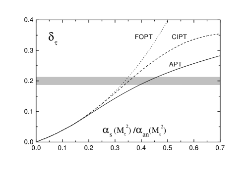
FIG. 1.: Behavior of the QCD perturbative contribution to $R_{\tau}$ as a function of $\alpha_{s}(M_{\tau}^{2})$ (for FOPT and CIPT) or of $\alpha_{\rm{an}}(M_{\tau}^{2})$ (for APT) in the $\overline{\rm{MS}}$ renormalization scheme.

In Fig. 1, we compare $\delta_{\tau}$ as a function of the three-loop running coupling in the cases of FOPT, CIPT, and APT. The running coupling in the Euclidean region is defined by

$$\alpha(Q^{2})=\frac{1}{\pi}\int_{0}^{\infty}\frac{d\sigma}{\sigma+Q^{2}}\mbox{Im}\left[\alpha_{\rm pt}(-\sigma-i\epsilon)\right],$$ (22)

which in lowest order coincides with Eq. (12). This plot corresponds to calculations in the $\overline{\rm{MS}}$-scheme. The difference between these functions is negligible at sufficiently small $\alpha_{s}(M_{\tau}^{2})$ and becomes substantial with larger values of the coupling. The shaded area reflects the value $\delta_{\tau}=0.200\pm 0.013$ [16] which corresponds to the experimental measurement for the non-strange channel of the $\tau$-data [17, 18].

A discussion of the perturbative contribution to inclusive $\tau$-decay has been given in Ref. [19], in which it has been claimed that in order to describe the experimental data for $\tau$-decay the value of $\alpha_{\rm{an}}(M_{\tau}^{2})$ should be taken in the range of $1.5$–$2.0$. This conclusion contradicts our result. Fig. 1 clearly demonstrates that in order to reproduce the experimental data such large values of $\alpha_{\rm{an}}(M_{\tau}^{2})$ are not required. Moreover, in the APT approach, the value of the analytic running coupling $\alpha_{\rm{an}}(Q^{2})$ is bounded from above and cannot exceed the infrared limiting value $\alpha_{\rm{an}}\leq\pi/\beta_{0}\simeq 1.4$ [3]. Beyond this, in Ref. [19], it was noted that this impossibly large value $\alpha_{\rm{an}}(M_{\tau}^{2})$ corresponds to $\alpha_{s}(M_{Z}^{2})\simeq 0.15$. However, in order to obtain the value of $\alpha_{s}$ at the $Z$-boson mass scale, the region of five active quarks should be approached by applying a special procedure of matching from the three-quark region [12, 13]. Corresponding estimates have been given in Ref. [10]. The large value of the scale parameter $\Lambda$ extracted in a pure APT analysis of the $\tau$-data indicates that nonperturbative effects are not negligible. As it has been demonstrated in Ref. [20], the light $D$-function corresponding to the non-strange vector channel $\tau$-data can be described by using reasonable effective quark masses with $\Lambda_{\overline{\rm{MS}}}\simeq 420$ MeV.

As has been emphasized in Ref. [19], the merit of the contour representation is that it produces expressions for quantities in the physical region that are not expansions in the parameter $\pi/\ln(\,s/\Lambda^{2})$, not a small quantity in the intermediate energy region. In particular, one can write the formula for $R(s)$ [see Eq. (11) from Ref. [19]] which contains the expression on the right-hand side of Eq. (13). Although we agree with the authors of Ref. [19] that it is important to sum up the $\pi^{2}$-terms in the region of intermediate energies (see Ref. [14]) and that it is preferable to use an expression which sums up the $\pi^{2}$-contributions rather than the asymptotic expression $\propto 1/\ln(s/\Lambda^{2})$, we note the following: The expression discussed in Ref. [19] is simply associated with the APT timelike function (13) which unambiguously leads to the Euclidean function (12). So, we conclude that the analytic approach provides a consistent form of expressions of the type (13) in the timelike region, whose evident advantage is the summation of the $\pi^{2}$-contributions into a regular function, and results in the corresponding analytic expressions for the $D$-function in the spacelike region, where unphysical singularities are cancelled by functions of a nonlogarithmic type vanishing in a perturbative expansion. In other words, summation of the $\pi^{2}$-contributions in the s-channel produces power (nonlogarithmic in $Q^{2}$) contributions in the t-channel that ensure the analytic properties by canceling unphysical singularities in the logarithmic terms.

A significant source of theoretical uncertainty of the results obtained arises from the RS dependence due to the inevitable inclusion of only a finite number of terms in the PT series. There are no general principles that give preference to a particular renormalization scheme and the stability of the result has to be studied at least with respect to a relevant class of schemes. A virtue of the APT approach is its higher stability over a wide range of RS [10]. (A similar observation has been made in the context of deep-inelastic scattering sum rules [8, 9].) In contrast, results obtained in the framework of FOPT have a strong RS dependence. Indeed, if one performs calculations in some scheme and then by using a RS transformation extracts the value of $\alpha_{s}^{\overline{\rm{MS}}}(M_{\tau}^{2})$ in the commonly used ${\overline{\rm{MS}}}$-scheme, we find that this value possesses a strong uncertainty. This fact is shown in Fig. 2. A point on the $(K_{1},b_{2})$-plane corresponds to a RS, where $b_{2}=\beta_{2}/\beta_{0}$ is the ratio of the three-loop and one-loop coefficients of the $\beta$-function. In the shaded area there are no appropriate solutions of the cubic equation (16). We indicate the popular ${\overline{\rm{MS}}}$ scheme and the optimal schemes: ECH, which recently has been applied to the $\tau$-decay [21], based on an effective charge method [22], and PMS based on a principle of minimal sensitivity [23]. A straightforward way of extracting the value of the coupling based solely on the ${\overline{\rm{MS}}}$ scheme gives $\alpha_{s}^{\overline{\rm{MS}}}(M_{\tau}^{2})=0.337\pm 0.008$. An analysis which takes into account the RS ambiguity leads to a much larger error in $\alpha_{s}(M_{\tau}^{2})$. The reason for the enhanced RS stability of the APT scheme is its perturbative stability—the leading order term captures the bulk of the QCD correction.

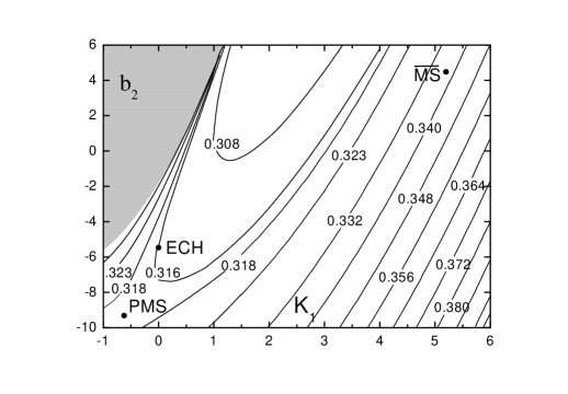
FIG. 2.: Contour plot of $\alpha_{s}^{\overline{\rm{MS}}}(M_{\tau}^{2})$ extracted from the $\tau$-data by using different renormalization schemes in the FOPT approach.

In summary, we have made a comparative analysis of the merits and drawbacks of three forms of perturbative approximations in the context of the application of QCD to the inclusive decay of the $\tau$-lepton. Two of them, the FOPT and CIPT, use, in one way or another, the running coupling with unphysical singularities to parameterize $R_{\tau}$. However, the justification of these schemes is rather different. The FOPT has a more solid foundation than the CIPT, which is simply self-contradictory. However, due to the strong RS dependence, the FOPT leads to a large uncertainty in extracting QCD parameters from the data. We have put forward arguments in favor of APT. Calculations in the framework of this approach are self-consistent and considerably reduce the theoretical uncertainty of the results obtained; this is important in extracting the nonperturbative component of the QCD description of the process.

The authors would like to thanks D.V. Shirkov for interest in this work and useful discussions. Partial support of the work by the U.S. Department of Energy, grant number DE-FG03-98ER41066, and by the RFBR, grants 99-01-00091, 99-02-17727, and 00-15-96691, is gratefully acknowledged.

REFERENCES

- [1] E. Braaten, Phys. Rev. Lett. 60, 1606 (1988); Phys. Rev. D 39, 1458 (1989).
- [2] F. Le Diberder and A. Pich, Phys. Lett. B 286, 147 (1992).
- [3] D.V. Shirkov and I.L. Solovtsov, Phys. Rev. Lett. 79, 1209 (1997).
- [4] K.A. Milton, I.L. Solovtsov, and O.P. Solovtsova, Phys. Lett. B 415, 104 (1997).
- [5] I.L. Solovtsov and D.V. Shirkov, Phys. Lett. B 442, 344 (1998).
- [6] D.V. Shirkov, Theor. Math. Phys. 119, 438 (1999).
- [7] I.L. Solovtsov and D.V. Shirkov, Theor. Math. Phys. 120, 1220 (1999).
- [8] K.A. Milton, I.L. Solovtsov, and O.P. Solovtsova, Phys. Lett. B 439, 421 (1998).
- [9] K.A. Milton, I.L. Solovtsov, and O.P. Solovtsova, Phys. Rev. D 60, 016001 (1999).
- [10] K.A. Milton, I.L. Solovtsov, O.P. Solovtsova, and V.I. Yasnov, Eur. Phys. J. C 14, 495 (2000).
- [11] K.A. Milton and I.L. Solovtsov, Phys. Rev. D 55, 5295 (1997).
- [12] K.A. Milton and O.P. Solovtsova, Phys. Rev. D 57, 5402 (1998).
- [13] D.V. Shirkov, Theor. Math. Phys. 127, 409 (2001).
- [14] D.V. Shirkov, Eur. Phys. J. C 22, 331 (2001).
- [15] G. Grunberg, hep-ph/9705290.
- [16] A. Pich, in: Proc. TAU 2000, edited by R.J. Sobie and J.M. Roney, Nucl. Phys. B (Proc. Suppl.) 98, 385 (2001).
- [17] ALEPH Collaboration, R. Barate et al., Eur. Phys. J. C 4, 409 (1998).
- [18] OPAL Collaboration, K. Ackerstaff et al., Eur. Phys. J. C 7, 571 (1999).
- [19] B.V. Geshkenbein, B.L. Ioffe, and K.N. Zyablyuk, Phys. Rev. D 64, 093009 (2001).
- [20] K.A. Milton, I.L. Solovtsov, and O.P. Solovtsova, Phys. Rev. D 64, 016005 (2001).
- [21] J.G. Krner, F. Krajewski, and A.A. Pivovarov, Phys. Rev. D 63, 036001 (2001).
- [22] G. Grunberg, Phys. Rev. D 29, 2315 (1984); A. Dhar and V. Gupta, Phys. Rev. D 29, 2822 (1984).
- [23] P.M. Stevenson, Phys. Rev. D 23, 2916 (1981).