RADIATIVE RETURN AT NLO AND THE
MEASUREMENT OF THE HADRONIC CROSS-SECTION

Abstract

The measurement of the hadronic cross-section in $e^{+}e^{-}$ annihilation at high luminosity factories using the radiative return method is motivated and discussed. A Monte Carlo generator which simulates the radiative process $e^{+}e^{-}\rightarrow\gamma+hadrons$ at the next-to-leading order accuracy is presented. The analysis is then extended to the description of events with hard photons radiated at very small angle.

TTP01-26

13.40.Em, 13.40.Ks, 13.65.+i

1 Motivation

Electroweak precision measurements in present particle physics provide a basic issue for the consistency tests of the Standard Model (SM) or its extensions. New phenomena physics can affect low energy processes through quantum fluctuations (loop corrections). Deviations from the SM predictions can therefore supply indirect information about new undiscovered particles or interactions.

The recent measurement of the muon anomalous magnetic moment $a_{\mu}\equiv(g-2)_{\mu}/2$ at BNL [1] reported a new world average showing a discrepancy at the $2.6$ standard deviation level with respect to the theoretical SM evaluation of the same quantity which has been taken as an indication of new physics. For the correct interpretation of experimental data the appropriate inclusion of higher order effects as well as a very precise knowledge of the SM input parameters is required. The BNL experiment plans a new measurement with an accuracy three times smaller which will challenge even more the theoretical predictions.

One of the main ingredients of the theoretical prediction for the muon anomalous magnetic moment is the hadronic vacuum polarization contribution which moreover is responsible for the bulk of the theoretical error. This quantity plays also an important role in the evolution of the electromagnetic coupling $\alpha_{QED}$ from the low energy Thompson limit to high energies. In both cases the precise knowledge of the ratio

$$R(s)=\frac{\sigma(e^{+}e^{+}\rightarrow hadrons)}{\sigma(e^{+}e^{-}\rightarrow\mu^{+}\mu^{-})}~{},$$ (1)

over a wide range of energies is required. The measurement of the hadronic cross section in $e^{+}e^{-}$ annihilation to an accuracy better than $1\%$ in the energy range below $2$ GeV is necessary to improve the accuracy of the present predictions for the muon anomalous magnetic moment and the QED coupling.

In this paper, the radiative return method is motivated and described. It has the advantage against the conventional energy scan [2], that the systematics of the measurement (e.g. normalization, beam energy) have to be taken into account only once but not for each individual energy point independently. An improved Monte Carlo generator which simulates the radiative process $e^{+}e^{-}\rightarrow\gamma+hadrons$ at the Next-to-Leading Order (NLO) accuracy is presented. Finally, the analysis is extended to the description of events with hard photons radiated at very small angle.

2 The muon anomalous magnetic moment and the QED coupling

The Standard Model prediction for the muon anomalous magnetic moment consist of three contributions 

$$a_{\mu}=a_{\mu}^{\mathtt{QED}}+a_{\mu}^{\mathtt{had}}+a_{\mu}^{\mathtt{weak}}~{}.$$ (2)

The QED correction, known (estimated) up to five loops [4], gives the main contribution (see Table 1 for numerical values ). The weak contribution is currently known up to two loops [5]. Finally, the hadronic contribution consist of three different terms where the leading one comes from the vacuum polarization diagram in figure 1 which furthermore is responsible for the bulk of the theoretical uncertainty.

	$a_{\mu}\times 10^{11}$
QED	116584706 $\pm$	3
hadronic ($\mathsf{vacuum\;polarization}$)	6924 $\pm$	62	[8]
hadronic ($\mathsf{light-by-light}$)	-85 $\pm$	25	[12]
hadronic ($\mathsf{other\;higher\;orders}$)	-101 $\pm$	6	[13]
weak	152 $\pm$	4

Table 1: QED, hadronic and weak contributions to the muon anomalous magnetic moment.

      

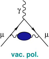
Figure 1: Vacuum polarization and light-by-light hadronic contributions to the muon anomalous magnetic moment.

While the QED and the weak contributions are well described perturbatively, the hadronic contribution cannot be completely calculated from perturbative QCD. The hadronic vacuum polarization contribution [6, 7, 8, 9, 10, 11] can however be evaluated from the following dispersion relation

$$\quad a_{\mu}^{\mathtt{had}}(\mathsf{vac.pol.})=\left(\frac{\alpha m_{\mu}}{3\pi}\right)^{2}\int_{4m_{\pi}^{2}}^{\infty}\frac{ds}{s^{2}}\;K(s)\;R(s)~{},$$ (3)

where the kernel $K(s)$ is a known smooth bounded function and $R(s)$ is the hadronic ratio which has to be extracted from experimental data. Under the assumption of conserved vector current and isospin symmetry $\tau$ decays can be included also for the evaluation of the dispersion integral. Due to the $1/s^{2}$ dependence of the dispersion integral, the low energy region contributes dominantly to this integral: $70\%$ of the result comes from the $\pi\pi$ channel and, even more, $90\%$ of it is given by the region below $1.8$ GeV. The precise measurement of the hadronic cross section in $e^{+}e^{-}$ annihilation, specially at low energies, has therefore a crucial importance for the accurate determination of the muon anomalous magnetic moment.

The running of the QED fine structure constant from the Thompson limit to high energies is given by

$$\alpha(s)=\frac{\displaystyle\alpha(0)}{\displaystyle 1-\Delta\alpha(s)}~{},\qquad\Delta\alpha=\Delta\alpha_{\mathtt{lep}}+\Delta\alpha_{\mathtt{top}}+\Delta\alpha_{\mathtt{had}}~{}.$$ (4)

Again, the Standard Model prediction consists of several contributions. Among them, the hadronic one which can be evaluated from the dispersion relation

$$\Delta\alpha_{\mathtt{had}}(s)=-\frac{\alpha s}{3\pi}Re\int_{4m_{\pi}^{2}}^{\infty} \frac{ds^{\prime}}{s^{\prime}}\;\frac{R(s^{\prime})}{s-s^{\prime}-i\eta}~{}.$$ (5)

The leptonic [14] and the top quark [15] contributions are well described perturbatively while the hadronic contribution [16] gives the main theoretical error (see Table 2 for numerical values). The dispersion integral grows in this case only as $1/s$ which means that also the high energy points become relevant. The region below $1.8$ GeV contributes only to $20\%$ of the integral. A better knowledge of the hadronic cross section in this region would be nevertheless also important to reduce the error.

	$\Delta\alpha(\mathsf{M_{Z}})\times 10^{4}$
leptonic	314.98
top quark	-0.70 $\pm$	0.05
hadronic	276.1   $\pm$	3.6

Table 2: Leptonic, top quark and hadronic contributions to the running of the QED fine structure constant at $M_{Z}$.

3 The radiative return method and the hadronic cross section

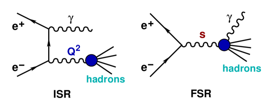
Figure 2: Initial state radiation (ISR) and final state radiation (FSR) in the annihilation process $e^{+}e^{-}\rightarrow\gamma+hadrons$.

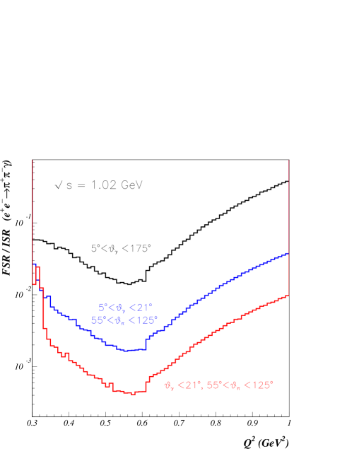
Figure 3: Relative contribution of FSR versus ISR in the annihilation process $e^{+}e^{-}\rightarrow\pi^{+}\pi^{-}\gamma$ at $\sqrt{s}=1.02$GeV for different photon and pion angular cuts. $E_{\gamma}>10$MeV.

The radiative process $e^{+}e^{-}\rightarrow\gamma+hadrons$, where the photon is radiated from the initial particles (initial state radiation, ISR), see figure 2, can be used to measure the hadronic cross section $\sigma(e^{+}e^{-}\rightarrow hadrons)$ at high luminosity electron-positron storage rings, like the $\phi$-factory DAPHNE or at $B$-factories, over a wide range of energies. The radiated photon reduces the effective energy of the collision and thus the invariant mass of the hadronic system. This possibility has been proposed and studied in detail in [17] (See also [18]). A Monte Carlo generator called EVA [17] which simulates the process $e^{+}e^{-}\rightarrow\pi^{+}\pi^{-}\gamma$ was built. The four pion channel was considered in [19].

Radiation of photons from the hadronic system (final state radiation, FSR) should be considered as the background of the measurement. One of the main issues of the radiative return method is the suppression of this kind of events by choosing suitable kinematical cuts. From EVA studies this is achieved by selecting events with the tagged photons close to the beam axis and well separated from the hadrons which reduces FSR to a reasonable limit. This is illustrated in figure 3. Furthermore, the suppression of FSR overcomes the problem of its model dependence which should be taken into account in a completely inclusive measurement [20].

Preliminary experimental results using the radiative return method have been presented recently by the KLOE collaboration [21]. Large event rates were also observed at BaBar [22].

The theoretical description of the radiative events under consideration to a precision better than $1\%$ requires a precise control of higher order radiative corrections. The next sections are devoted to the calculation of the NLO corrections to ISR and its inclusion in a new improved Monte Carlo generator [24, 25].

4 NLO corrections to ISR

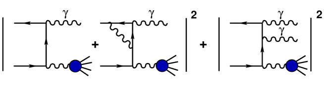
Figure 4: NLO corrections to initial state radiation in the annihilation process $e^{+}e^{-}\rightarrow\gamma+hadrons$.

At NLO, the $e^{+}e^{-}$ annihilation process

$$e^{+}(p_{1})+e^{-}(p_{2})\rightarrow \gamma^{*}(Q)+\gamma(k_{1})~{},$$ (6)

where the virtual photon decays into a hadronic final state, $\gamma^{*}(Q)\rightarrow$ hadrons, and the real one is emitted from the initial electron or positron, receives contributions from one-loop corrections and from the emission of a second real photon (see figure 4 for a schematic representation).

The calculation of the different contributions proceeds as follows: first the one-loop diagrams are reduced, using the standard Passarino-Veltman procedure [23], to the calculation of a few one-loop scalar integrals which are calculated in $D=4-2\epsilon$ dimensions in order to regularize their divergences. The interference with the lowest order Feynman diagrams is calculated and the ultraviolet (UV) divergences are renormalized using the on-shell mass scheme. The remaining infrared (IR) divergences are cancelled by adding the soft contribution of the second photon calculated analytically by integration in phase space up to a soft energy cutoff $E_{\gamma}<w\sqrt{s}$ far below the center of mass energy $\sqrt{s}$.

In order to facilitate the extension of the Monte Carlo simulation to different hadronic exclusive channels the differential rate is cast into the product of a leptonic and a hadronic tensor and the corresponding factorized phase space

$$d\sigma=\frac{1}{2s}L_{\mu\nu}H^{\mu\nu}d\Phi_{2}(p_{1},p_{2};Q,k_{1})d\Phi_{n}(Q;q_{1},\cdot,q_{n})\frac{dQ^{2}}{2\pi}~{},$$ (7)

where $d\Phi_{n}(Q;q_{1},\cdot,q_{n})$ denotes the hadronic $n$-body phase-space including all statistical factors and $Q^{2}$ is the invariant mass of the hadronic system. The physics of the hadronic system, whose description is model dependent, enters only through the hadronic tensor $H^{\mu\nu}$.

The leptonic tensor which describes the next-to-leading order virtual and soft QED corrections to initial state radiation in $e^{+}e^{-}$ annihilation has the following general form:

$$L^{\mu\nu}_{\mathrm{virt+soft}} =\frac{(4\pi\alpha)^{2}}{Q^{4}\;y_{1}\;y_{2}}\;\bigg{[}a_{00}\;g^{\mu\nu}+a_{11}\;\frac{p_{1}^{\mu}p_{1}^{\nu}}{s}+a_{22}\;\frac{p_{2}^{\mu}p_{2}^{\nu}}{s}$$

$$+a_{12}\;\frac{p_{1}^{\mu}p_{2}^{\nu}+p_{2}^{\mu}p_{1}^{\nu}}{s}+i\pi\;a_{-1}\;\frac{p_{1}^{\mu}p_{2}^{\nu}-p_{2}^{\mu}p_{1}^{\nu}}{s}\bigg{]}~{},$$ (8)

where $y_{i}=2k_{1}\cdot p_{i}/s$ with $p_{1}$ ($p_{2}$) the four momentum of the positron (electron). The scalar coefficients $a_{ij}$ and $a_{-1}$ allow the following expansion

$$a_{ij}=a_{ij}^{(0)}+\frac{\alpha}{\pi}\;a_{ij}^{(1)}~{},\qquad a_{-1}=\frac{\alpha}{\pi}\;a_{-1}^{(1)}~{},$$ (9)

where $a_{ij}^{(0)}$ give the LO contribution. The NLO coefficients $a_{ij}^{(1)}$ and $a_{-1}^{(1)}$ were calculated in [24] for the case where the observed photon is far from the collinear region. The extension of these results to the forward and backward regions is commented in Section 6.

Finally, the contribution from radiation of two real hard photons, $E_{\gamma}>w\sqrt{s}$, is calculated numerically using the helicity amplitude method [26]. The sum of the virtual plus soft corrections to one single photon events and the hard contribution of two photon emission gives the final result at NLO which is independent of the soft photon cutoff $w$.

5 Monte Carlo simulation

A Monte Carlo generator has been built which simulates the production of two charged pions together with one or two hard photons and includes virtual and soft photon corrections to the emission of one single real photon. It supersedes the previous versions of the EVA [17, 24] Monte Carlo. Again the program exhibits a modular structure which preserves the factorization of the initial state QED corrections. The simulation of other exclusive hadronic channels can, therefore, be easily included with the simple replacement of the current(s) of the existing modes, and the corresponding multi-particle hadronic phase space. The simulation of the four pion channel [19] will be incorporated soon as well as other multi-hadron final states. Our results will be presented in [25].

6 Tagged or untagged photons

From the experimental point of view it would be much easier to perform the analysis with no lower photon angular boundary. The cross section in the forward and backward regions grows very fast and therefore a small deviation in the determination of the photon angle could introduce a large error. It turns out that further advantages appear if only an upper cut on the photon angle is imposed. The cross section is thus larger. For instance, the cross section for radiative events with $\theta_{\gamma}<21^{\circ}$ and $55^{\circ}<\theta_{\pi}<125^{\circ}$ is 4 times bigger than the corresponding cross section for $5^{\circ}<\theta_{\gamma}<21^{\circ}$. Furthermore, since FSR is isotropic with respect to the beam axis its contribution does not change much and, as a result, its relative importance with respect to ISR is much smaller (see lower line in figure 3). All together may provide a better control of the systematics of the measurement and, therefore, a better determination of the hadronic cross section.

It should be point out that in the forward and backward regions some corrections of order $m_{e}^{2}/s$, where $m_{e}$ is the electron mass, has to be taken into account even though $m_{e}^{2}/s$ is a small quantity. At LO, the full leptonic tensor is given by:

$$L_{0}^{\mu\nu} =\frac{(4\pi\alpha/s)^{2}}{q^{4}}\;\bigg{[}\left(\frac{2m^{2}q^{2}(1-q^{2})^{2}}{y_{1}^{2}y_{2}^{2}}-\frac{2q^{2}+y_{1}^{2}+y_{2}^{2}}{y_{1}y_{2}}\right)g^{\mu\nu}$$

$$+\left(\frac{8m^{2}}{y_{2}^{2}}-\frac{4q^{2}}{y_{1}y_{2}}\right)\frac{p_{1}^{\mu}p_{1}^{\nu}}{s}+\left(\frac{8m^{2}}{y_{1}^{2}}-\frac{4q^{2}}{y_{1}y_{2}}\right)\frac{p_{2}^{\mu}p_{2}^{\nu}}{s}$$

$$-\left(\frac{8m^{2}}{y_{1}y_{2}}\right)\frac{p_{1}^{\mu}p_{2}^{\nu}+p_{1}^{\nu}p_{2}^{\mu}}{s}\bigg{]}~{},$$ (10)

with $y_{i}=2k_{1}\cdot p_{i}/s$, $m^{2}=m_{e}^{2}/s$ and $q^{2}=Q^{2}/s$. Expressing the bilinear products $y_{i}$ by the photon emission angle in the center of mass frame

$$y_{1,2}=\frac{1-q^{2}}{2}(1\mp\beta\cos\theta)~{},\qquad\beta=\sqrt{1-4m^{2}}~{}.$$

The electron mass enters twofold. Through $y_{i}$, $i=1,2$, but also quadratically in terms of the type $m^{2}/y_{i}^{2}$. In the former case, the electron mass regulates the collinear divergences of the cross section. The second kind of contributions gives only finite corrections which, nevertheless, can be sizeable. In both cases the electron mass plays a relevant role only when the photon is emitted at very small angles. Otherwise, the limit $m_{e}^{2}/s\rightarrow 0$ can be taken safely.

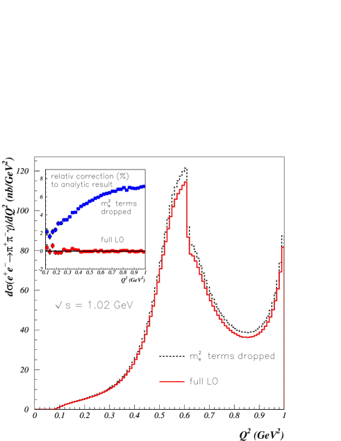
Figure 5: Effect of the quadratic terms in the electron mass in the LO prediction for the $e^{+}e^{-}\rightarrow\pi^{+}\pi^{-}\gamma$ differential distribution. $E_{\gamma}>10$ MeV.

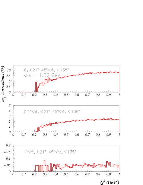
Figure 6: Electron mass corrections for different photon angular cuts.

To illustrate this point the differential cross section for the process $e^{+}e^{-}\rightarrow\pi^{+}\pi^{-}\gamma$ at $\sqrt{s}=1.02$ GeV is presented in figure 5. The pion and photon angles are integrated without applying any angular cut. The electron mass is kept in the scalar bilinears $y_{i}$ but the quadratic terms are considered or not to show their effect. Both results are compared in the small insert of this figure with the known corresponding analytical differential distribution

$$Q^{2}\frac{d\sigma}{dQ^{2}}=\frac{4\alpha^{3}}{3s}R(Q^{2})\bigg{\{}\frac{s^{2}+Q^{4}}{s(s-Q^{2})}\left(\log\frac{s}{m_{e}^{2}}-1\right)\bigg{\}}~{},$$ (11)

with the substitution $R(Q^{2})\rightarrow(1-4m_{\pi}^{2}/Q^{2})^{3/2}$ $\mid~{}F_{2\pi}(Q^{2})\mid^{2}/4$ for the two pion exclusive channel, being $F_{2\pi}$ the pion form factor. In (11) the expansion in the electron mass has been performed after integration. Figure 5 shows thus the good performance of the Monte Carlo integration also at very small photon angles. The analytical result agrees with the Monte Carlo integration when the full electron mass dependence is considered in Eq.(10). If the quadratic mass terms are not taken into account a deviation of up to $8\%$ is found. In contrast, at higher energies these corrections are quite suppressed, less than 1 per mil at $\sqrt{s}=10$ GeV.

Figure 6 shows the effect of the electron mass corrections for different angular cuts at $\sqrt{s}=1.02$ GeV. Up to $10\%$ deviation with respect to the full result is found which nevertheless decreases quite steeply if the collinear region is excluded: to less than 5 per mil for tagged photon events at $1$ degree minimal angle.

These electron mass finite corrections, which are relevant only in the very forward and backward regions, below 1 degree at $\sqrt{s}=1.02$ GeV, have been included in the new version of the EVA Monte Carlo. At present, only at LO. At NLO, the corresponding electron mass corrections to the virtual and soft contributions in one photon events are included in the definition of the $y_{i}$’s while the quadratic terms will be included soon. For two photon events the full electron mass dependence is already considered.

7 Conclusions

The radiative return method is a competitive method to measure the hadronic cross section at high luminosity $e^{+}e^{-}$ colliders ($\phi$ and $B$-factories) giving access to a wide range of energies, from threshold to the center of mass energy of the collider. A Monte Carlo generator has been built which simulates the production of two charged pions together with one or two hard photons and includes virtual and soft photon corrections to the emission of one single real photon. Its modular structure is such that the simulation of other exclusive hadronic channels can be easily included. The description of events with hard photons radiated at very small angle has been also investigated.

It is a pleasure to thank the organizers of this meeting for the stimulating atmosphere created during the school and the Katowice group for his kind hospitality. The author acknowledges J. H. Kühn and H. Czyż for a fruitful collaboration. Work supported in part by BMBF under grant number 05HT9VKB0, E.U. EURODAPHNE network TMR project FMRX-CT98-0169 and E.U. TMR grant HPMF-CT-2000-00989.

References

- [1] H. N. Brown et al. [Muon g-2 Collaboration], Phys. Rev. Lett. 86 (2001) 2227 [hep-ex/0102017].
- [2] R. R. Akhmetshin et al. [CMD-2 Collaboration], [hep-ex/9904027].
- [3] J. Prades, [hep-ph/0108192]. K. Melnikov, [hep-ph/0105267]. W. J. Marciano and B. L. Roberts, [hep-ph/0105056].
- [4] V. W. Hughes and T. Kinoshita, Rev. Mod. Phys. 71 (1999) S133. A. Czarnecki and W. J. Marciano, Nucl. Phys. Proc. Suppl. 76 (1999) 245 [hep-ph/9810512].
- [5] T. V. Kukhto, E. A. Kuraev, Z. K. Silagadze and A. Schiller, Nucl. Phys. B 371 (1992) 567. S. Peris, M. Perrottet and E. de Rafael, Phys. Lett. B 355 (1995) 523 [hep-ph/9505405]. A. Czarnecki, B. Krause and W. J. Marciano, Phys. Rev. D 52 (1995) 2619 [hep-ph/9506256]; Phys. Rev. Lett. 76 (1996) 3267 [hep-ph/9512369].
- [6] S. Eidelman and F. Jegerlehner, Z. Phys. C 67 (1995) 585 [hep-ph/9502298].
- [7] D. H. Brown and W. A. Worstell, Phys. Rev. D 54 (1996) 3237 [hep-ph/9607319].
- [8] M. Davier and A. Höcker, Phys. Lett. B 435 (1998) 427 [hep-ph/9805470].
- [9] S. Narison, Phys. Lett. B 513 (2001) 53 [hep-ph/0103199].
- [10] F. Jegerlehner, [hep-ph/0104304].
- [11] J. F. De Trocóniz and F. J. Ynduráin, [hep-ph/0106025].
- [12] E. de Rafael, Phys. Lett. B 322 (1994) 239 [hep-ph/9311316]. J. Bijnens, E. Pallante and J. Prades, Nucl. Phys. B 474 (1996) 379 [hep-ph/9511388]; Phys. Rev. Lett. 75 (1995) 1447 [Erratum-ibid. 75 (1995) 3781] [hep-ph/9505251]. M. Hayakawa and T. Kinoshita, Phys. Rev. D 57 (1998) 465 [hep-ph/9708227]. M. Hayakawa, T. Kinoshita and A. I. Sanda, Phys. Rev. D 54 (1996) 3137 [hep-ph/9601310]; Phys. Rev. Lett. 75 (1995) 790 [hep-ph/9503463].
- [13] B. Krause, Phys. Lett. B 390 (1997) 392 [hep-ph/9607259].
- [14] M. Steinhauser, Phys. Lett. B 429 (1998) 158 [hep-ph/9803313].
- [15] J. H. Kühn and M. Steinhauser, Phys. Lett. B 437 (1998) 425 [hep-ph/9802241]. K. G. Chetyrkin, J. H. Kühn and M. Steinhauser, Phys. Lett. B 371 (1996) 93 [hep-ph/9511430].
- [16] H. Burkhardt and B. Pietrzyk, LAPP-EXP-2001-03.
- [17] S. Binner, J. H. Kühn and K. Melnikov, Phys. Lett. B459 (1999) 279 [hep-ph/9902399]. K. Melnikov, F. Nguyen, B. Valeriani and G. Venanzoni, Phys. Lett. B477 (2000) 114 [hep-ph/0001064].
- [18] S. Spagnolo, Eur. Phys. J. C 6 (1999) 637. V. A. Khoze, M. I. Konchatnij, N. P. Merenkov, G. Pancheri, L. Trentadue and O. N. Shekhovzova, Eur. Phys. J. C 18 (2001) 481 [hep-ph/0003313].
- [19] H. Czyż and J. H. Kühn, Eur. Phys. J. C 18 (2001) 497 [hep-ph/0008262].
- [20] A. Höfer, J. Gluza and F. Jegerlehner, [hep-ph/0107154].
- [21] A. Aloisio et al. [KLOE Collaboration], [hep-ex/0107023]. A. Denig et al. [KLOE Collaboration], eConf C010430 (2001) T07 [hep-ex/0106100]. M. Adinolfi et al. [KLOE Collaboration], [hep-ex/0006036].
- [22] E. P. Solodov [BABAR collaboration], eConf C010430 (2001) T03 [hep-ex/0107027].
- [23] G. Passarino and M. Veltman, Nucl. Phys. B 160 (1979) 151.
- [24] G. Rodrigo, A. Gehrmann-De Ridder, M. Guilleaume and J. H. Kühn, Eur. Phys. J. C DOI 10.1007/s100520100784 [hep-ph/0106132].
- [25] G. Rodrigo, H. Czyż, J. H. Kühn and M. Szopa, in preparation.
- [26] F. Jegerlehner and K. Kołodziej, Eur. Phys. J. C 12 (2000) 77 [hep-ph/9907229]. K. Kołodziej and M. Zrałek, Phys. Rev. D 43 (1991) 3619.
- [27] M. Knecht, A. Nyffeler, M. Perrottet and E. d. Rafael, [hep-ph/0111059]. M. Knecht and A. Nyffeler, [hep-ph/0111058].