Robust signatures of solar neutrino oscillation solutions

Robust signatures of solar neutrino oscillation solutions

Abstract:

With the goal of identifying signatures that select specific neutrino oscillation parameters, we test the robustness of global oscillation solutions that fit all the available solar and reactor experimental data. We use three global analysis strategies previously applied by different authors and also determine the sensitivity of the oscillation solutions to the critical nuclear fusion cross section, $S_{17}(0)$, for the production of ${\rm{}^{8}B}$. Our standard results make use of the precise new measurement of $S_{17}(0)$ by Junghans et al. The globally favored solutions are, in order of goodness of fit: LMA(the only solution at $2\sigma$), LOW, and VAC. The NC to CC ratio for SNO is predicted by the standard global analysis to be $3.45^{+0.70}_{-0.54}(1\sigma)$ which is separated from the no-oscillation value of $1.0$ by much more than the expected experimental error. The predicted range of the day-night difference in CC rates is $8.3^{+5.0}_{-5.6}(1\sigma)$%. A measurement by SNO of either a NC to CC ratio $>3.3$ or a day-night difference $>10$%, would favor a small region of the currently allowed LMA neutrino parameter space. The global oscillation solution predicts a ${\rm{}^{7}Be}$ neutrino-electron scattering rate in BOREXINO and KamLAND in the range $0.65^{+0.04}_{-0.03}(1\sigma)$ of the BP00 standard solar model rate, a prediction which can be used to test both the solar model and the neutrino oscillation theory. Only the LOW solution predicts a large day-night effect($\leq 42$%, $3\sigma$) in BOREXINO and KamLAND. For the reactor KamLAND experiment, the LMA solution predicts a charged current rate relative to the standard model of $0.44^{+0.22}_{-0.07}(1\sigma),~{}~{}E_{\rm threshold}=1.22{\rm~{}MeV}$. We have also evaluated the effects of including preliminary Super-Kamiokande data for $1496$ days of observations.

1 Introduction

How robust are the predictions of the allowed neutrino oscillation solutions that are obtained by fitting the currently available solar neutrino data with different neutrino oscillation parameters? How can we determine experimentally the neutrino oscillation parameters? We address these questions in the present paper.

To determine the robustness of the oscillation solutions and their predicted experimental consequences, we compute the currently allowed regions in neutrino oscillation space using three different analysis strategies, each strategy previously advocated by a different set of authors. We include all the available solar neutrino and reactor oscillation data [1, 2, 3, 4, 5, 6, 7]. We also present “Before and After” comparisons of the globally allowed solutions using both the previous(1998) standard value of $S_{17}(0)$,the low energy cross section factor for the production of ${\rm{}^{8}B}$, and a precise new measurement [8] for this important quantity.

In order to identify which quantities are most likely to lead to an experimental determination of the neutrino oscillation parameters, we use the allowed regions in neutrino parameter space to predict the expected range of the most promising quantities that can be measured accurately in solar neutrino experiments. For the Sudbury Neutrino Observatory (SNO) [7, 9], we report the predictions of the currently allowed regions for the neutral current to charged current double ratio, [NC]/[CC], the day-night effect, and the first and second moments of the electron recoil energy spectrum. For experiments like BOREXINO  [10] and KamLAND [11] that can detect ${\rm{}^{7}Be}$ solar neutrinos, we evaluate the predicted range of the neutrino-electron scattering rate and the difference between the night and the day event rates.

It pays to be lucky. We show in figure 11 and figure 14 that if SNO measures (as predicted by some LMA oscillation parameters) a large value for either the neutral current to charged current ratio or the day-night difference in rates, or if BOREXINO or KamLAND measures(as predicted by some LOW oscillation parameters) a large day-night difference, then this measurement will uniquely select the correct neutrino oscillation solution and fix the neutrino oscillation parameters to within rather small uncertainties. On the other hand, a small value of the neutral current to charged current ratio would favor the SMA solution.

How should this paper be read? Since you got this far, we recommend that you now turn to the final section, the summary and discussion section, and see what results seem most interesting to you. The summary and discussion section refers to what we believe are the most useful figures and tables, which the reader may wish to glance at before deciding whether to invest the time to read the detailed text in the main sections.

This paper is organized as follows. In section 2 we present the predicted solar neutrino fluxes and their uncertainties that are derived from the BP00 standard solar model [12] with and without including the recent precise measured value for $S_{17}(0)$ determined by Junghans et al. [8]. We determine in section 3 the regions in neutrino oscillation parameter space that are allowed using three different analysis scenarios; we present results obtained using both the new value for $S_{17}(0)$ and the previous(1998) standard value. We use the three sets of global oscillation solutions in section 4 to determine for SNO the $3\sigma$ (and $1\sigma$) ranges of predicted values for the neutral current to charged current ratio, the difference between the day and the night CC event rates, and the first two moments of the energy spectrum of the CC recoil electrons. In section 5, we determine for the BOREXINO and KamLAND solar neutrino experiments the $3\sigma$ (and $1\sigma$) ranges of allowed values for the neutrino-electron scattering rate and the day-night effect. For the reactor KamLAND experiment, we present in section 6 the predicted $3\sigma$ (and $1\sigma$) ranges of the charged current (antineutrino absorption) rate and the distortion of the visible energy spectrum. We summarize and discuss our conclusions in section 7.

We use, unless stated otherwise, the techniques and parameters for the analysis that we have described elsewhere [13, 14, 15, 16].

2 BP00 + New ${\rm\bf{}^{8}B}$

In this section, we present the predicted solar neutrino fluxes (table 1) and their uncertainties (table 2) that were computed with the BP00 solar model [12], with and without taking account of a recent precise measurement of the production cross section that leads to the emission of ${\rm{}^{8}B}$ neutrinos. Both the solar neutrino fluxes and their uncertainties are used in calculations of the allowed regions for neutrino oscillation parameters.

There has been a lot of beautiful experimental work devoted to measuring the rate of the fusion reaction ${\rm{}^{7}Be(p,\gamma)^{8}B}$ [8, 17]. Recent experiments have concentrated on reducing the systematic uncertainties, in going to lower center-of-mass energies that are more relevant to the sun, and in using new measurement techniques. The goal is to reduce the uncertainty in the low energy cross section factor for the reaction ${\rm{}^{7}Be(p,\gamma)^{8}B}$ to less than or equal to $5$% [18], so that it is no longer the dominant uncertainty in the prediction of the ${\rm{}^{8}B}$ solar neutrino flux. Very important experiments are continuing to be performed on this reaction.

The recent Junghans et al. precision measurement of the low energy cross section for the fusion reaction ${\rm{}^{7}Be(p},\gamma){\rm{}^{8}B}$ yields [8]

$$S_{17}(0)=\left(22.3\pm 0.7\left({\rm expt}\right)\pm 0.5\left({\rm theor}\right)\right){\rm eVb}.$$ (1)

The quoted uncertainty for the Junghans et al. measurement, which combines statistical and systematic uncertainties, is smaller than for all previous low energy measurements. Other relatively recent measurements [17] have yielded values of $S_{17}(0)$ that are smaller than the Junghans et al. value.

For illustrative purposes, we adopt in this paper $S_{17}(0)=\left(22.3\pm 0.9\right){\rm eVb}$ instead of the previous(1998) standard value of $S_{17}(0)=19^{+4}_{-2}{\rm eVb}$ [19] that was used in the original calculations [12] of the BP00 standard model neutrino fluxes. The value of $S_{17}(0)$ given in eq. (1) is $0.8\sigma$ larger than the previously used value.

We will present throughout this paper the differences in the calculated quantities that result from using $S_{17}(0)=\left(22.3\pm 0.9\right){\rm eVb}$ instead of $S_{17}(0)=19^{+4}_{-2}{\rm eVb}$. These two values of $S_{17}(0)$ span the set of recent experimental results [8, 17].

2.1 Fluxes

Table 1: Standard Model Predictions (BP00 + New ${\rm{}^{8}B}$): solar neutrino fluxes and neutrino capture rates, with $1\sigma$ uncertainties from all sources (combined quadratically). The neutrino fluxes are the same as in the original BP00 model [12] except for the ${\rm{}^{8}B}$ flux, which is increased because of the larger adopted value of $S_{17}(0)$, see eq. (1). Using the 1998 standard value $S_{17}(0)=19^{+4}_{-2}{\rm eVb}$ [19], the ${\rm{}^{8}B}$ neutrino flux was calculated previously to be $\phi\left({\rm{}^{8}B}\right)=5.05\left(1.00^{+0.20}_{-0.16}\right)$. The total rates were calculated using the neutrino absorption cross sections and their uncertainties that are given in ref. [20]

Source	Flux	Cl	Ga
	$\left(10^{10}\ {\rm cm^{-2}s^{-1}}\right)$	(SNU)	(SNU)
pp	$5.95\times 10^{0}~{}~{}\left(1.00^{+0.01}_{-0.01}\right)$	0.00	69.7
pep	$1.40\times 10^{-2}\left(1.00^{+0.015}_{-0.015}\right)$	0.22	2.8
hep	$9.3\times 10^{-7}$	0.04	0.1
${\rm{}^{7}Be}$	$4.77\times 10^{-1}\left(1.00^{+0.10}_{-0.10}\right)$	1.15	34.2
${\rm{}^{8}B}$	$5.93\times 10^{-4}\left(1.00^{+0.14}_{-0.15}\right)$	6.76	14.2
${\rm{}^{13}N}$	$5.48\times 10^{-2}\left(1.00^{+0.21}_{-0.17}\right)$	0.09	3.4
${\rm{}^{15}O}$	$4.80\times 10^{-2}\left(1.00^{+0.25}_{-0.19}\right)$	0.33	5.5
${\rm{}^{17}F}$	$5.63\times 10^{-4}\left(1.00^{+0.25}_{-0.25}\right)$	0.00	0.1
Total		$8.59^{+1.1}_{-1.2}$	$130^{+9}_{-7}$

Any plausible change in the value of $S_{17}(0)$ has no discernible numerical effect on the standard solar model [18]. The reaction ${\rm{}^{7}Be(p},\gamma){\rm{}^{8}B}$ is so rare (it occurs of order twice in every $10^{4}$ completions of the $p-p$ chain) that even a factor of ten change in the cross section does not affect, to the required accuracy, the calculated solar model temperatures and densities. The $15$% increase in the best-estimate value of $S_{17}(0)$ represented by eq. (1) does not change significantly any of the computed physical variables in the standard solar model except the ${\rm{}^{8}B}$ neutrino flux.

For a given solar model with specified distributions of temperature, density, and composition, the calculated ${\rm{}^{8}B}$ neutrino flux depends [18] linearly upon the adopted value of $S_{17}(0)$, i.e., $\phi({\rm{}^{8}B})\propto S_{17}(0)$.

Table 1 presents the predicted neutrino fluxes, and the predicted chlorine and gallium capture rates, for the BP00 standard solar model and the ${\rm{}^{7}Be(p},\gamma){\rm{}^{8}B}$ cross section factor of eq. (1). Except for $\phi({\rm{}^{8}B})$, all of the fluxes in table 1 are the same as in table 7 of the original BP00 paper [12].

2.2 Uncertainties

Table 2 summarizes the uncertainties in the most important solar neutrino fluxes and in the Cl and Ga event rates that are due to different nuclear fusion reactions (the first four entries), the heavy element to hydrogen mass ratio (Z/X), the radiative opacity, the solar luminosity, the assumed solar age, and the helium and heavy element diffusion coefficients. In addition, the ${\rm{}^{14}N}+p$ reaction causes a $0.2$% uncertainty in the predicted pp flux, a $0.1$ SNU uncertainty in the Cl event rate, and a $1$ SNU uncertainty in the Ga event rate.

The uncertainty in the laboratory measurement of the low energy cross section factor for the ${\rm{}^{3}He}$(${\rm{}^{4}He}$,$\gamma$)${\rm{}^{7}Be}$ reaction is the dominant uncertainty in the calculation of the ${\rm{}^{7}Be}$ neutrino flux and one of the two largest uncertainties in the calculation of the ${\rm{}^{8}B}$ neutrino flux.

For the original BP00 solar model predictions [12], the uncertainties in the individual parameters and in the fluxes are, with the exception of the two non-zero entries in the column under ${\rm{}^{7}Be+p}$, the same as in table 2. Instead of the entries $0.040$ under ${\rm{}^{7}Be+p}$, the original BP00 model predictions had a much larger uncertainty, $0.105$. The original BP00 uncertainties were used, for example, in the analyses of solar neutrino oscillations described in refs.  [13, 16, 21, 22].

The input data that were used to calculate the uncertainties listed in table 2 are given in the papers in which the BP00 model [12] and the BP98 model [23] were originally presented. The principal change from the uncertainties that were calculated for the BP98 model (cf. table 2 in ref. [23]), and which were used in many previous analyses of solar neutrino oscillations, is that, assuming the validity of eq. (1), the uncertainty in the cross section for the ${\rm{}^{7}Be(p},\gamma){\rm{}^{8}B}$ reaction is reduced by a factor of more than three and the estimated uncertainty in the heavy element to hydrogen ratio, $Z/X$, is increased by almost a factor of two( cf. discussion in section 5.1.2 of ref. [12]).

The predicted event rates for the chlorine and gallium experiments make use of neutrino absorption cross sections from refs. [20]. The uncertainty in the prediction for the standard (no oscillation) gallium rate is dominated by uncertainties in the neutrino absorption cross sections, $7$ SNU ($5$% of the predicted rate). The uncertainties in the chlorine absorption cross sections cause an error, $\pm 0.22$ SNU ($2.6$% of the predicted rate), that is relatively small compared to other uncertainties in predicting the rate for this experiment. For calculations that involve non-standard neutrino energy spectra that result from neutrino oscillations or other new neutrino physics, the uncertainties in the predictions for currently favored solutions (which reduce the contributions from the least well-determined ${\rm{}^{8}B}$ neutrinos) will in general be less than the values quoted here for standard spectra and must be calculated using the appropriate cross section uncertainty for each neutrino energy [20].

Table 2: For the standard solar model (BP00 + New ${\rm\bf{}^{8}B}$), the average uncertainties in neutrino fluxes and event rates due to different input data. The flux uncertainties are expressed in fractions of the total flux and the event rate uncertainties are expressed in SNU. The ${\rm{}^{7}Be}$ electron capture rate causes an uncertainty of $\pm 2\%$ [24] that affects only the ${\rm{}^{7}Be}$ neutrino flux. The average fractional uncertainties for individual parameters are shown.

$<$Fractional	pp	${\rm{}^{3}He^{3}He}$	${\rm{}^{3}He^{4}He}$	${\rm{}^{7}Be}+p$	$Z/X$	opac	lum	age	diffuse
uncertainty$>$	0.017	0.060	0.094	0.040	0.061		0.004	0.004	0.15
Flux
pp	0.002	0.002	0.005	0.000	0.004	0.003	0.003	0.0	0.003
${\rm{}^{7}Be}$	0.016	0.023	0.080	0.000	0.034	0.028	0.014	0.003	0.018
${\rm{}^{8}B}$	0.040	0.021	0.075	0.040	0.079	0.052	0.028	0.006	0.040
SNUs
Cl	0.3	0.2	0.6	0.3	0.6	0.4	0.2	0.04	0.3
Ga	1.3	1.0	3.3	0.6	3.1	1.8	1.3	0.20	1.5

3 Global neutrino oscillation solutions with different analysis prescriptions

We present in this section the global solutions for the allowed neutrino oscillation parameters that are derived using the neutrino fluxes and uncertainties given in table 1 and table 2. We describe in section 3.1 the oscillation solutions that are allowed with three different analysis prescriptions (see figure 1) and show how adopting the new Junghans et al. value of $S_{17}(0)$ reduces the allowed regions in neutrino parameter space (see figure 2). We have at different times used all three of the analysis strategies and various colleagues have advocated strongly one or the other of the strategies described here. In section 3.3, we describe in more detail the three different analysis prescriptions. Section 3.1 is intended for a general readership, while section 3.3 is intended primarily for aficionados of neutrino oscillations.

The interested reader may wish to consult also a number of recent papers, refs. [16, 21, 22, 25, 26, 27], that have determined the allowed solar neutrino oscillation solutions including the CC data from SNO. We will spare the reader erudite comparisons, in the cases where there is overlap in the calculated quantities, between our detailed results and those of the other authors referred to above. In general, when the same analysis procedures and input data are used, all authors obtain consistent results.

In this paper, we study the sensitivity of the calculated neutrino predictions to the adopted analysis strategy by comparing the numerical results obtained with three different analysis procedures. We also compare, for global neutrino solutions and for predicted neutrino measurable quantities, the results that are obtained using the previous standard value for $S_{17}(0)$ with the results that are obtained using the recent precise measurement by Junghans et al. [8] of $S_{17}(0)$. In our previous paper on solar neutrino oscillations [16], we used only the analysis strategy (a) (cf. Section 3.3 for a description of all three analysis strategies) and the previously standard value for $S_{17}(0)$. We apply the sensitivity studies described in section 3 to the calculation of a variety of solar neutrino measurables in sections 4-6, providing for the first time a quantitative evaluation of the robustness of the predictions to diverse analysis strategies.

3.1 Global oscillation solution: three different analyses

Figure 1: Global neutrino oscillation solutions for three different analysis strategies. The three different analysis strategies are described in section 3.3. In all cases, the value of $S_{17}(0)$ reported in ref.   [8] and shown in eq. (1) was used. The input data include the neutrino fluxes and uncertainties predicted by the BP00 solar model [12] and the total measured event rates from the SNO [7], Chlorine [1], and Gallium (averaged) [2, 3, 4] experiments, as well as the recoil electron energy spectrum measured by Super-Kamiokande [5] during the day and separately the energy spectrum measured at night. The C.L. contours shown in the figure are $90$%, $95$%, $99$%, and $99.73$% ($3\sigma$). The allowed regions are limited by the Chooz reactor measurements [6] to mass values below $\sim$ (7–8) $\times 10^{-4}{\rm eV^{2}}$. The local best-fit points are marked by dark circles.

We first discuss in section 3.1.1 the new global solutions for each of three different analysis strategies and then compare in section 3.1.2 the global solutions that are obtained with the older and newer (cf. eq. 1) values of $S_{17}(0)$.

3.1.1 New global solution

Figure 1 shows the allowed ranges of the neutrino oscillation parameters, $\Delta m^{2}$ and $\tan^{2}\theta$, that were computed following three different analysis approaches that have been used previously in the literature. These approaches are described in more detail in section 3.3. We follow refs. [28, 29] in using $\tan^{2}\theta$ (rather than $\sin^{2}2\theta$) in order to display conveniently solutions on both sides of $\theta=\pi/4$.

Figure 1a presents the result for our standard analysis, which includes the BP00 predicted fluxes and uncertainties and all the experimental data except the Super-Kamiokande total event rate. The measured day and night electron recoil energy spectra together represent the Super-Kamiokande total rate in this approach. Figure 1b was constructed using an analysis similar to that used to construct figure 1a except that for figure 1b the total Super-Kamiokande rate is included explicitly together with a free normalization factor for the day and night recoil energy spectra. Figure 1c shows the results for the free ${\rm{}^{8}B}$ analysis, in which the calculation is the same as for the standard case, figure 1a, except that the ${\rm{}^{8}B}$ neutrino flux is not constrained by the solar model predictions.

The allowed regions obtained in the three panels of figure 1, although different, do not depend dramatically on the adopted strategy. The allowed regions are reduced in size for strategy (a) and strategy (b) as compared to the regions derived using the 1998 standard value of $S_{17}(0)$ [19], cf. the results presented in refs. [16] and  [22], respectively.

The most restricted allowed regions are obtained for strategy (b), which has been used by the Bari group [22]. As discussed in ref.[16], the smallness of the allowed regions for this strategy results from the absence in the analysis of the ${\rm{}^{8}B}$ theoretical error for the Super-Kamiokande spectrum normalization. We will discuss this point more in the next section.

The largest allowed regions in figure 1 correspond to strategy (c), used among others by Krastev and Smirnov [21], in which the ${\rm{}^{8}B}$ neutrino flux is treated as a free parameter. This was not the case when using the 1998 standard value of $S_{17}(0~{}\cite[cite]{[\@@bibref{}{adelberger}{}{}]})$ (see fig.9 in ref [16]). The only changes in the quantities derived from BP00 and BP00 + New ${\rm{}^{8}B}$ are the ${\rm{}^{8}B}$ neutrino flux and its associated uncertainty. Therefore the allowed regions are unchanged when going from BP00 to BP00 + New ${\rm{}^{8}B}$ in strategy (c), for which the ${\rm{}^{8}B}$ neutrino flux is treated as a free parameter. Thus Fig. 1c is equal to the right panel of Fig.9 in Ref. [16] and it is also in excellent agreement with the results from the free ⁸B analysis of ref. [21]. The change in the relative size of the allowed regions between strategy (a) and (c) is due to the reduction in size, discussed above, of the allowed regions for strategy (a).

In constructing figure 1, we assumed that only active neutrinos exist. We derive therefore the allowed regions in $\chi^{2}$ using only two free parameters: $\Delta m^{2}$ and $\tan^{2}\theta$. As discussed below, oscillations into pure sterile neutrinos are highly disfavored (see table 3) with the larger value of $S_{17}(0)$ given in eq. (1), and are not included in our standard demarcation of the allowed regions. The allowed regions for a given C.L. are defined in this paper as the set of points satisfying the condition

$$\chi^{2}(\Delta m^{2},\theta)-\chi^{2}_{\rm min}\leq\Delta\chi^{2}\mbox{(C.L., 2~{}d.o.f.)},$$ (2)

with $\Delta\chi^{2}(\mbox{C.L., 2~{}d.o.f.})=4.61$, $5.99$, $9.21$, and $11.83$ for C.L. = 90%, 95%, 99% and 99.73% ($3\sigma$). We use the standard least-square analysis approximation for the definition of the allowed regions with a given confidence level. As shown in ref. [26] the allowed regions obtained in this way are very similar to those obtained by a bayesian analysis.

Table 3: Best-fit global oscillation parameters with all solar neutrino data. The table gives for the global solution illustrated in figure 1a the best-fit values for $\Delta m^{2}$, $\tan^{2}\theta$, $\chi^{2}_{\rm min}$, and g.o.f. for all the neutrino oscillation solutions that were discussed in our previous analysis in ref. [16]. The differences of the squared masses are given in ${\rm eV^{2}}$. The number of degrees of freedom is 39 [38(19 night spectrum, 19 day spectrum) + 3(rates) $-$2(parameters: $\Delta{\rm m}^{2}$, $\theta$)]. The BP00 best-fit fluxes and their estimated errors have been included in the analysis (see table 1 and table 2). The rates from the GALLEX/GNO and SAGE experiments have been averaged to provide a unique data point. The goodness-of-fit given in the last column is calculated from the value of $\chi^{2}/{\rm d.o.f}$ at each local minimum (i.e., for LMA, SMA, VAC). Solutions that have $\chi_{\rm min}^{2}\geq 34.5+11.83$ are not allowed at the $3\sigma$ C.L.

Solution	$\Delta m^{2}$	$\tan^{2}(\theta)$	$\chi^{2}_{\rm min}$	g.o.f.
LMA	$3.7\times 10^{-5}$	$3.7\times 10^{-1}$	34.5	$67$%
LOW	$1.0\times 10^{-7}$	$6.7\times 10^{-1}$	40.8	$39$%
VAC	$4.6\times 10^{-10}$	$2.5\times 10^{0}$	42.3	$33$%
Sterile VAC	$4.7\times 10^{-10}$	$3.0\times 10^{0}$	49.1	$13$%
SMA	$5.2\times 10^{-6}$	$1.8\times 10^{-3}$	49.9	$11$%
Just So2	$5.5\times 10^{-12}$	$0.61(1.6)\times 10^{0}$	52.1	$7.8$%
Sterile Just So2	$5.5\times 10^{-12}$	$0.61(1.6)\times 10^{0}$	52.1	$7.8$%
Sterile SMA	$4.6\times 10^{-6}$	$3.4\times 10^{-4}$	52.3	$7.5$%

Table 3 gives for our standard analysis strategy (cf. figure 1a) the best-fit values for $\Delta m^{2}$ and $\tan^{2}\theta$ for all the neutrino oscillation solutions that were discussed in our previous analysis in ref. [16]. The table also lists the values of $\chi_{\rm min}^{2}$ for each solution. The regions for which the local value of $\chi_{\rm min}^{2}$ exceeds the global minimum by more than $11.83$ are not allowed at $3\sigma$ C.L. Thus, all solutions with $\chi_{\rm min}^{2}$ as bad or worse than the VAC Sterile solution are not allowed at $3\sigma$ for the standard analysis.

The set of allowed solutions at $3\sigma$ C. L. would not change if we considered active-sterile admixtures and defined the allowed regions as in figure 1 of ref. [16] in terms of $\Delta\chi^{2}(\mbox{C.L., 3~{}d.o.f.})$ instead of $\Delta\chi^{2}(\mbox{C.L., 2~{}d.o.f.})$. Table 3 shows that all regions with $\Delta\chi^{2}>11.83$ (corresponding to $3\sigma$ C.L. for $2$ d.o.f.) also satisfy $\Delta\chi^{2}>14.16$ (corresponding to $3\sigma$ C.L. for $3$ d.o.f.).

Many authors(see, e. g., ref. [30] and references quoted therein) have discussed the possibility of bi-maximal neutrino oscillations, which in the present context implies $\tan^{2}\theta=1$. Figure 1 shows that bi-maximal mixing is disfavored for the preferred LMA solution. Quantitatively, we find that there there are no solutions with $\tan^{2}\theta=1$ at the $99.87$% C.L. for our standard analysis strategy, corresponding to panel (a) of figure 1. For the strategies corresponding to the panels (b) and (c), respectively, there are no solutions with $\tan^{2}\theta=1$ at the $99.95$% C.L. and $98.95$% confidence level. Maximal mixing is allowed for the less favored LOW and VAC solutions at a C.L. that varies between $95$% and $3\sigma$, depending upon the analysis strategy. In summary, maximal mixing is not favored but it is not rigorously ruled out.

The upper limit on on the allowed value of $\Delta m^{2}$ is important for neutrino oscillation experiments, as stressed in ref. [21]. In units of $10^{-4}~{}{\rm eV^{2}}$. we find the following $3\sigma$ upper limits on $\Delta m^{2}$ (values in parenthesis are obtained with the older value of $S_{17}(0)$, see ref. [19]): case a: 4.7 (7.5); case b: 3.0 (6.8); and case c: 6.5 (6.5). The upper limit therefore lies between $3.0$ and $7.5$, in units of $10^{-4}~{}{\rm eV^{2}}$, depending upon what is assumed about $S_{17}(0)$ and the analysis strategy.

3.1.2 Global “Before and After”

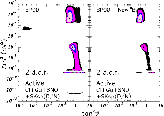
Figure 2: Global “Before and After.” The left panel shows the allowed regions for the neutrino oscillations computed in ref. [16] (see figure 9a of that paper) with $S_{17}(0)=19^{+4}_{-2}{\rm eVb}$ [19] and the standard analysis procedure used here(cf. figure 1) and in ref. [16]. The right panel, which is the same as figure 1a, shows the allowed regions computed with the same procedure but with the Junghans et al. value of $S_{17}(0)=(22.3\pm 0.9){\rm eVb}$ [8].

Figure 2 compares the allowed regions found with the new ${\rm{}^{8}B}$ theoretical neutrino flux and uncertainties (table 1 and table 2) with our previously published results(see figure 9a of , ref. [16]). We like to refer to this comparison as our global “Before-After” figure.

The modification of the ${\rm{}^{8}B}$ flux and uncertainties considered in this paper results in a reduction of the allowed neutrino oscillation parameter space. Since no pure sterile oscillation solutions are found at the $3\sigma$ level, we focus on oscillations involving only active neutrinos. We find allowed regions for the LMA, LOW, and VAC solutions with our standard analysis strategy. The allowed regions for the preferred LMA and LOW solutions both become smaller with the larger adopted $S_{17}(0)$, and the fit to the LOW solution becomes relatively less good. The SMA and Just-so² solutions, which are marginally allowed in the standard ’Before’ panel of figure 2, are not present in the ’After’ panel at the 3-$\sigma$ level.

The differences between the Before and After panels are mainly due to two effects, which are described below.

(a)

The increase of the ${\rm{}^{8}B}$ normalization results in a smaller value for $\chi^{2}_{\rm min}$, which is found for the LMA best-fit point. With the new value of $S_{17}(0)$, we find $\chi^{2}({\rm LMA})_{\rm min}=34.5$ while before we had $\chi^{2}({\rm LMA})_{\rm min}=35.3$. Although the theoretical errors are reduced in the new solution, the global minimum (which lies within the boundaries of the LMA solution) is “deeper.” This effect can be confirmed by comparing the results of figure 1a and figure 1c, which were computed with and without the BP00 constraint on the ${\rm{}^{8}B}$ neutrino flux. The global minimum points are much closer together in neutrino parameter space than they were when the older value of $S_{17}(0)$ was used (cf. results given in ref. [16]). With the new ${\rm{}^{8}B}$ normalization the LMA best-fit point is not only the best-fit point in oscillation parameter space but it also corresponds very closely to the predicted ${\rm{}^{8}B}$ neutrino flux given in table 1. We find that $\phi({\rm{}^{8}B};{\rm LMA~{}best-fit})=0.999\phi({\rm{}^{8}B};{\rm BP00+New^{8}B})$, where the coefficient $0.999$ applies for case (c) (free ${\rm{}^{8}B}$ analysis). For our standard analysis, case (a), the coefficient is $0.96$. Presumably, this precise agreement between the best-fit LMA neutrino flux and the BP00 + New ${\rm{}^{8}B}$ flux is accidental, since the allowed $3\sigma$ range for the ${\rm{}^{8}B}$ flux, within the domain of the LMA oscillation parameters, is $(0.54-1.36)\phi({\rm{}^{8}B};{\rm BP00+New^{8}B})$.

(b)

The theoretical error for the ${\rm{}^{8}B}$ flux is reduced according to eq. (1) from an average value of $19$% with the Adelberger et al. value of $S_{17}(0)$ [19] to $14.5$% with the Junghans et al. value [8] of $S_{17}(0)$. The reduction of this theoretical error pushes the previously marginally allowed SMA and Just So² solutions (for these somewhat unfamiliar solutions see the original discovery papers [31] and ref. [13]) over the edge (beyond the $3\sigma$ allowed region). As discussed in section 5.3 of ref. [16], the error on the predicted ${\rm{}^{8}B}$ neutrino flux played a crucial role in previously allowing, with the standard analysis prescription, the marginal SMA and Just So² solutions.

We have performed a series of numerical experiments to determine which effect, either the increase in the predicted ${\rm{}^{8}B}$ flux or the decrease in the uncertainty in the predicted flux, is the dominant effect in reducing the allowed parameter space. We find that the increase in the predicted flux contributes the most to worsening the fit for the LOW solution while the decrease in the uncertainty in the predicted flux is dominant reason why the SMA and Just So² regions no longer appear at $3\sigma$. The increase in the predicted flux and the decrease in the theoretical uncertainty contribute comparably to reducing the size of the LMA allowed region.

3.2 The allowed range for the ${\rm{}^{8}B}$ neutrino flux

The analysis described above yields best-estimates and $3\sigma$ allowed ranges for the total ${\rm{}^{8}B}$ neutrino flux. Let $f_{\rm B}$ be the inferred ${\rm{}^{8}B}$ neutrino flux produced in the sun in units of the best-estimate predicted BP00 neutrino flux,

$$f_{\rm B}~{}=~{}\frac{\phi({\rm{}^{8}B})}{\phi({\rm{}^{8}B})_{\rm BP00+New^{8}B}}.$$ (3)

Table 4 gives the best-estimate and allowed range of the solar ${\rm{}^{8}B}$ neutrino flux. The values in brackets in table 4 were obtained by our standard analysis, case (a), while the values without brackets were derived allowing the ${\rm{}^{8}B}$ neutrino flux to be a free parameter, i. e., case (c). The bracketed range is always slightly smaller than the unbracketed range, which just reflects the fact that for strategy (a) the $\chi^{2}$ penalizes large differences from the standard solar model value of the ⁸B flux while the ⁸B flux is unconstrained for strategy (c). However, the two strategies, (a) and (c), yield similar allowed ranges for $f_{\rm B}$.

In all cases, the inferred range of $f_{\rm B}$ allowed by the global oscillation analysis using data from all of the experiments is smaller than the allowed range obtained by the SNO collaboration [7] from comparing the SNO and Super-Kamiokande total rate measurements. In our notation, the SNO collaboration found $f_{\rm B}=0.92\pm 0.50$, where the result is expressed in terms of the BP00 flux calculated with the Junghans et al. value of $S_{17}(0)$ (see table 1 and ref. [8]) and we quote the $3\sigma$ allowed range. Our result is $f_{\rm B}=0.88\pm 0.48$[or, for strategy (a), $f_{\rm B}=0.86\pm 0.38$]. Of course, the SNO determination is more direct. The procedure described here assumes the validity of the two-neutrino oscillation analysis and uses solar model fluxes and uncertainties (see especially discussion in section 7.1).

Even when the ${\rm{}^{8}B}$ neutrino flux is unconstrained in the oscillation analysis, almost all of the allowed range of $f_{\rm B}$ is within the $3\sigma$ uncertainty of the BP00 solar model predictions. Only for the SMA solution does the allowed range of $f_{\rm B}$ not overlap with the $3\sigma$ predicted range of the BP00 solar model.

The procedure described above assumes the validity of the two-neutrino oscillation analysis for pure active oscillations. As shown in ref. [25], the allowed range of $f_{\rm B}$ can be modified by allowing for the possibility of an admixture of sterile neutrinos in the oscillations within the adiabatic regime. In order to test this possibility we have repeated our global analysis (c) with an arbitrary active-sterile admixture within the region $10^{-3}<\Delta m^{2}/{\rm eV}^{2}<10^{-5}$ , $0.05<\tan^{2}\theta<5$. We find that the maximum allowed ${\rm{}^{8}B}$ neutrino flux is increased to $f_{\rm B}\leq 2.9$ (at 3$\sigma$ for 3 d.o.f.) and corresponds to oscillations into a $25$% active and $75$% sterile state. However, these mixed scenarios including sterile neutrinos give a worse fit to the data than pure active oscillations. A large component of sterile neutrinos does better if one includes in the analysis only the total event rates, as in ref. [25]. For completeness, we briefly describe how this is possible. In order to fit the appearance of active neutrinos at Super-Kamiokande versus SNO, one needs to decrease $P_{ee}$ for ${\rm{}^{8}B}$ neutrinos [32] (which is compensated by the increase of $f_{\rm B}$ ), while in order to keep the agreement with gallium and chlorine rates the survival probability at lower energies must not be substantially modified. Barger et al. have pointed out in ref.  [25] that this tuning can be achieved within the adiabatic regime. However, as discussed in ref.  [16], one has less freedom for tuning in the global analysis. Within the adiabatic regime, the tuning of the probability can only be achieved by lowering both the value of $\tan^{2}\theta$ and $\Delta m^{2}$, intruding into the region of a predicted large day-night variation in the Super-Kamiokande experiment.

Table 4: Allowed values for the ${\rm{}^{8}B}$ neutrino flux. The table gives for each allowed oscillation solution the best-fit values for $f_{\rm B}$ and the $3\sigma$ range of allowed values. The quantity $f_{\rm B}$ is the ${\rm{}^{8}B}$ neutrino flux expressed in units of the best-estimate BP00 value for the ${\rm{}^{8}B}$ neutrino flux, see eq. (3). The values of $f_{\rm B}$ given in brackets were obtained by our standard analysis procedure, (a); the values presented without brackets were obtained by analysis procedure (c), in which the ⁸B flux is not constrained by solar model predictions.

Solution	$f_{\rm B}({\rm Best})$	$f_{\rm B}(3\sigma{\rm~{}range})$
LMA	$1.00$	$0.54-1.36\;[0.57-1.24]$
LOW	$0.73$	$0.54-0.93\;[0.55-0.91]$
VAC	$0.59$	$0.48-0.68\;[0.48-0.66]$
SMA	$0.44$	$0.40-0.50\;$[ no   solution]

3.3 Methods of analysis

In this subsection, we describe the implementations of the three different analysis strategies that were used to construct figure 1 and figure 2. For most readers, the outline of the analysis strategies given in section 3.1.1 will be sufficient. Section 3.3 is intended only for aficionados of solar neutrino oscillation studies.

The results shown in figure 1 and figure 2 were derived using the CC event rate measured by SNO [7], the Chlorine [1] and Gallium event rates [2, 4, 3] (we use here the weighted averaged of the GALLEX/GNO and SAGE rates), and the $2\times 19$ bins of the (1258 day) Super-Kamiokande [5] electron recoil energy spectrum measured separately during the day and night periods. We include, as described below, the predicted neutrino fluxes and their uncertainties, table 1 and table 2 of the present paper, for the standard solar model [12] (BP00 + New ${\rm{}^{8}B}$). We use the distribution for neutrino production fractions and the solar matter density given in ref. [12] and tabulated in http://www.sns.ias.edu/$\sim$jnb.

In order to explore the robustness of the inferred allowed regions in neutrino parameter space, we obtain the permitted regions using calculations based upon three different plausible prescriptions for the statistical analysis that have been used in the published literature and which we label as follows.

(a)

For our “standard” analysis, we adopt the prescription described in refs. [13, 16]. We do not include here the Super-Kamiokande total rate, since to a large extent the total rate is represented by the flux in each of the spectral energy bins. We define the $\chi^{2}$ function for the global analysis as:

$$\chi^{2}_{\rm global,a}=\sum_{i,j=1,41}(R^{th}_{i}-R^{\exp}_{i})\sigma_{G,ij}^{-2}(R^{th}_{j}-R^{\exp}_{j}),$$ (4)

where $\sigma_{G,ij}^{2}=\sigma_{R,ij}^{2}+\sigma_{SP,ij}^{2}$. Here $\sigma_{R,ij}$ is the corresponding $41\times 41$ error matrix containing the theoretical as well as the experimental statistical and systematic uncorrelated errors for the 41 rates while $\sigma_{SP,ij}$ contains the assumed fully–correlated systematic errors for the $38\times 38$ submatrix corresponding to the Super-Kamiokande day–night spectrum data. We include here the energy independent systematic error which is usually quoted as part of the systematic error of the total rate. The error matrix $\sigma_{R,ij}$ includes important correlations arising from the theoretical errors of the solar neutrino fluxes, or equivalently of the solar model parameters. We follow the principles described by the Bari group [33] in including the solar model uncertainties, using the updated data presented in table 2.

(b)

For the “all rates” analysis, we follow the prescription described in refs. [22, 33, 34, 14, 32]. In this approach, we use all the total event rates in the analysis, including the Super-Kamiokande total event rate with its corresponding theoretical error. We define the $\chi^{2}$ function for this global analysis as:

$$\chi^{2}_{\rm global,b}=\chi^{2}_{\rm Rates,b}+\chi^{2}_{\rm SP,b},$$ (5)

where

$$\chi^{2}_{\rm Rates,b} = \sum_{i,j=1,4}(R^{th}_{i}-R^{\exp}_{i})\tilde{\sigma}_{R,ij}^{-2}(R^{th}_{j}-R^{\exp}_{j}),$$ (6)

$$\chi^{2}_{\rm SP,b} = \sum_{i,j=1,38}(\alpha_{\rm SP}R^{th}_{i}-R^{\exp}_{i})\tilde{\sigma}_{SP,ij}^{-2}(\alpha_{\rm SP}R^{th}_{j}-R^{\exp}_{j}).$$ (7)

In $\chi^{2}_{\rm Rates}$, we include the CC event rate measured at SNO [7], the Chlorine [1] and Gallium [2, 3, 4] event rates and the Super-Kamiokande [5] total event rate. The matrix $\tilde{\sigma}_{R,ij}$ contains the theoretical uncertainties, as well as the experimental statistical and systematic errors, for the total rates. In particular, $\tilde{\sigma}_{R,ij}$ includes the energy independent systematic error for the Super-Kamiokande rate. On the other hand, the matrix $\tilde{\sigma}_{{\rm SP},ij}$ contains both the statistical as well as the systematic errors (both those that are correlated with energy and those that are uncorrelated) of the $38$ spectral energy data; $\tilde{\sigma}_{{\rm SP},ij}$ does not include the theoretical error of the ${\rm{}^{8}B}$ flux.

In order to avoid double counting, we allow a free normalization (for which no theoretical error is included) for the Super-Kamiokande day and night electron recoil energy spectra. Following the usual procedure for this approach, we introduce an arbitrary normalization factor, $\alpha_{\rm SP}$, for the amplitude of the energy spectra. For each value of the oscillation parameters $\chi^{2}_{{\rm global},b}$ is minimized with respect to $\alpha_{\rm SP}$.

(c)

The “free ${\rm{}^{8}B}$” analysis is identical to our standard analysis, described in (a) above, except that the ${\rm{}^{8}B}$ neutrino flux is not constrained by solar model predictions. This freedom is implemented by multiplying the ${\rm{}^{8}B}$ flux contribution to the $R^{th}_{i}$ in eq. (4) by the normalization factor, $f_{\rm B}$, and removing the theoretical ${\rm{}^{8}B}$ flux errors from $\sigma_{R,ij}$. In this case, the resulting $\chi^{2}$ function can also be written as

$$\chi^{2}_{\rm global,c}=\chi^{2}_{\rm Rates,c}+\chi^{2}_{\rm SP,c},$$ (8)

where

$$\chi^{2}_{\rm Rates,c} = \sum_{i,j=1,3}(R^{th}_{i}(f_{\rm B})-R^{\exp}_{i})\hat{\sigma}_{R,ij}^{-2}(R^{th}_{j}(f_{\rm B})-R^{\exp}_{j}),$$ (9)

$$\chi^{2}_{\rm SP,c} = \sum_{i,j=1,38}(R^{th}_{i}(f_{\rm B})-R^{\exp}_{i})\hat{\sigma}_{SP,ij}^{-2}(R^{th}_{j}(f_{\rm B})-R^{\exp}_{j}).$$ (10)

In $\chi^{2}_{\rm Rates,c}$, we include only the CC event rates measured in the SNO, Chlorine, and Gallium experiments. For these three rates, the error matrix $\hat{\sigma}_{R,ij}$ only differs from $\tilde{\sigma}_{R,ij}$ due to the absence of the theoretical error for the ⁸B neutrino flux. The error matrix $\hat{\sigma}_{SP,ij}$ only differs from $\tilde{\sigma}_{SP,ij}$ by the inclusion of the energy independent systematic error, which is usually quoted as part of the systematic error of the total rate.

For each value of the oscillation parameters, $\chi^{2}_{\rm global,b}$ is minimized with respect to $f_{\rm B}$. Notice that the only difference in the “free ${\rm{}^{8}B}$” analysis when performed in terms of BP00 or in terms of BP00 + New ${\rm{}^{8}B}$ is a shift in the corresponding best value of $f_{\rm B}$ for each value of the oscillation parameters $f_{\rm B}\rightarrow f_{\rm B}\left(\frac{5.05}{5.93}\right)$; the allowed regions are left unchanged as can be seen by comparing Fig. 1c with the right panel of Fig.9 in Ref. [16].

4 Predictions for SNO

In this section, we present the predictions for the Sudbury Neutrino Experiment (SNO), ref. [7], of the currently allowed neutrino oscillation solutions (cf. figure 1) for the neutral current to charged current ratio (section 4.1), for the CC day-night effect (section 4.2), for the $\nu_{e}+e$ day-night effect (section 4.3), and for the first and second moments of the electron recoil energy spectrum (section 4.4). In Section 4.5, we show that the neutrino oscillation parameters will be well determined if we are lucky and SNO measures a large value ($>3.3$) of the neutral current to charged current ratio or a large value ($>0.1$) for the day-night effect.

The SNO collaboration is studying charged current (CC) neutrino absorption by deuterium,

$$\nu_{e}+d\to p+p+e^{-}\ ,$$ (11)

as well as the neutral current (NC) neutrino disassociation of deuterium,

$$\nu_{x}+d\to n+p+\nu^{\prime}_{x}\ ,\quad(x=e,\mu,\,\tau).$$ (12)

SNO is the only operating (or completed) solar neutrino experiment that determines a CC rate for electrons whose energies are measured. The SNO neutral current detection is also unique. In addition, SNO measures neutrino-electron scattering,

$$\nu_{x}+e\to e+\nu^{\prime}_{x}\ ,\quad(x=e,\mu,\,\tau).$$ (13)

The statistical uncertainties for neutrino-electron scattering in the SNO detector are less favorable than those available from the Super-Kamiokande experiment [5].

Figure 3: The neutral current to charged current double ratio, [NC]/[CC] . The double ratio, [NC]/[CC], is defined by eq. (14). The three panels of predictions in figure 3 were derived from the $3\sigma$ ranges shown in the three panels of global solutions illustrated in figure 1 and obtained using the three analysis strategies described in section 3. Figure 3 was constructed using a $6.75$ MeV total electron energy for the CC threshold. Table 5 shows that, within the allowed domain of neutrino oscillation solutions, the value of [NC]/[CC] is not sensitive to the threshold energy adopted for the CC reactions. The tiny $3\sigma$ estimated measuring error in the left hand panel assumes the systematic uncertainties projected in ref. [35] and $3000$ CC events and $1200$ NC events. The ultimate SNO measurement will probably be even more precise than this estimate.

The predicted measurable effects for SNO have been investigated in detail in ref. [35] for the larger range of neutrino oscillation solutions that were viable prior to the publication [7] of the first SNO results on the rate of the CC reaction. We follow here the notation and the techniques described in ref. [35], concentrating on those effects that were shown previously to be the most likely to be measurable. We do not repeat here calculations of the effects that were discussed in ref. [35] and found to be small, such as the neutral current day-night effect or the seasonal difference (winter-summer difference).

Table 5: SNO Neutral Current to Charged Current Double Ratio and Day-Night CC Asymmetry. The table presents the double ratio, ${\rm[NC]/[CC]}$ and $A_{\rm N-D}$ (in %). The results are tabulated for different neutrino oscillation scenarios and for two different thresholds of the recoil electron kinetic energy used in computing the CC ratio, $4.5$ MeV (columns two through four) and $6.75$ MeV (columns five through seven). The ranges are obtained for the 3$\sigma$ regions for analysis (a).

	b.f.	max	min	b.f.	max	min
Scenario	4.5 MeV	4.5 MeV	4.5 MeV	6.75 MeV	6.75 MeV	6.75 MeV
	[NC]/[CC]	[NC]/[CC]	[NC]/[CC]	[NC]/[CC]	[NC]/[CC]	[NC]/[CC]
LMA	3.44	5.28	1.79	3.45	5.28	1.82
LOW	2.39	3.22	1.71	2.37	3.20	1.71
VAC	1.76	2.06	1.43	1.82	2.17	1.46
	AN-D	AN-D	AN-D	AN-D	AN-D	AN-D
LMA	7.4	19.5	0.0	8.3	21.4	0.0
LOW	4.3	10.4	0.0	3.7	9.5	0.0
VAC	0.1	0.3	-0.2	0.2	0.5	-0.3

For the CC reaction, we adopt a $6.75$ MeV kinetic energy threshold for the recoil electrons, the threshold used by the SNO collaboration in their CC measurement reported in ref. [7], as the standard value used in the figures. In order to illustrate the dependence upon the CC threshold, we also present results in the tables that refer to a $4.5$ MeV recoil electron kinetic energy threshold.

4.1 The Neutral Current to Charged Current Double Ratio

In this subsection, we present predictions for the ratio of neutral current events (NC) to charged current events (CC) in SNO. The most convenient form in which to discuss this quantity is [36]

$${\rm{[NC]}\over{[CC]}}={{\left({\rm(NC)_{Obs}/(NC)_{SM}}\right)}\over{\left({\rm(CC)_{Obs}/(CC)_{SM}}\right)}}.$$ (14)

The ratio ${\rm{[NC]}/{[CC]}}$ is equal to unity if nothing happens to the neutrinos after they are produced in the center of the sun (no oscillations occur). Also, ${\rm{[NC]}/{[CC]}}$ is independent of all solar model considerations provided that only one neutrino source, ⁸B, contributes significantly to the measured rates. Inserting into eq. (25) of ref. [35] the $3\sigma$ upper limit measured for the $hep$ flux by the Super-Kamiokande collaboration [5], one finds that $hep$ neutrinos affect the value of ${\rm{[NC]}/{[CC]}}$ by less than $0.05$% for a $4.5$ MeV CC kinetic energy threshold (and by less than $2$% for a $6.75$ MeV CC threshold.) Moreover, the calculational uncertainties due to the interaction cross sections and to the shape of the ⁸B neutrino energy spectrum are greatly reduced by forming the double ratio [37, 38, 39, 40].

Figure 3 and table 5 present the calculated range of the double ratios for the oscillation solutions that are currently allowed at $3\sigma$. The table gives the best-fit values for ${\rm{[NC]}/{[CC]}}$ as well as the maximum and minimum allowed double ratios for a threshold recoil electron kinetic energy for the CC reaction of $4.5$ MeV and separately for a CC threshold of $6.75$ MeV. The calculated double ratio is insensitive to the CC threshold within the range of thresholds that are considered.

The $1\sigma$ predicted range for our standard global analysis strategy (a) is $3.45^{+0.70}_{-0.54}$ for a CC threshold of $6.75$ MeV($3.44^{+0.70}_{-0.55}$ for a $4.75$ MeV threshold). The predicted range for analysis strategy (b) is slightly smaller and for analysis strategy (c) is somewhat larger ( $3.65^{+0.97}_{-0.80}$).

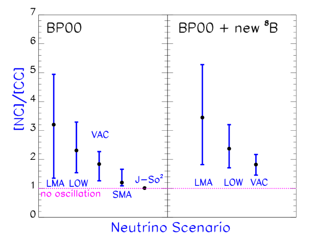
Figure 4: [NC]/[CC] “Before and After.” The left panel shows the $3\sigma$ allowed ranges for the neutral current to charged current double ratio using the neutrino oscillations solutions computed in ref. [16] with $S_{17}(0)=19^{+4}_{-2}{\rm eVb}$ [19] and the standard analysis procedure used here(cf. figure 1) and in ref. [16]. The right panel, which is the same as figure 3a, shows the allowed values for [NC]/[CC] computed with the same procedure but with the Junghans et al. value of $S_{17}(0)=(22.3\pm 0.9){\rm eVb}$ [8].

The best-fit values for the double ratio for oscillations into active neutrinos range between $1.8$ and $3.4$ ($1.8$ and $3.5$) for a $4.5$ MeV ($6.75$ MeV) CC threshold. The maximum predicted value for ${\rm{[NC]}/{[CC]}}$ is an enormous $5.3$ for an extreme LMA solution. The minimum calculated value for the double ratio is $1.4$, which is implied by an extreme VAC solution.

Figure 4 compares the “Before” and “After” predicted values for the neutral current to charged current double ratio. For the favored three solutions, LMA, LOW, and VAC, the predicted double ratios are not very sensitive to the precise value of $S_{17}(0)$ that is adopted. We note however that in all three cases adopting the Junghans et al. value of $S_{17}(0)$ causes the values of [NC]/[CC] to become slightly larger (more distant from the no oscillation value of $1.0$) as a consequence of the reductions and shifts of the allowed regions.

4.2 The Charged Current Day-Night Effect

Figure 5: The percentage difference between the night and the day CC rates. The figure shows the night-day percentage difference for the charged current rate in SNO, i.e., $100\times A_{\rm N-D}$ defined in eq. (15). Predictions are shown for the solar neutrino oscillation scenarios allowed at $3\sigma$ and illustrated in figure 1. The three panels refer to results for different analysis strategies described in section 3. Figure 5 was constructed using a recoil electron kinetic energy threshold of $6.75$ MeV for the CC events. Table 5 gives numerical results for $A_{\rm N-D}$ for kinetic energy thresholds of $4.5$ MeV and $6.75$ MeV.

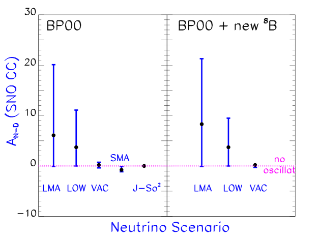
Figure 6: Night-Day CC “Before and After.” The left panel shows the $3\sigma$ allowed ranges in percent for the average CC night minus the day event rates, $A_{\rm N-D}$, as defined in eq. (15); the values in the left panel were computed using the neutrino oscillations solutions in ref. [16] obtained with $S_{17}(0)=19^{+4}_{-2}{\rm eVb}$ [19] and the standard analysis procedure used here(cf. figure 1) and in ref. [16]. The right panel, which is the same as figure 5a, shows the allowed values for $A_{\rm N-D}$ computed with the same procedure but with the Junghans et al. value of $S_{17}(0)=(22.3\pm 0.9){\rm eVb}$ [8].

In this subsection, we discuss the difference between the charged current event rate observed at night and the charged current event rated observed during the day. This difference in event rates has been evaluated previously for a variety of experiments by many authors, including those listed in refs [36, 35, 41, 21, 42].

We concentrate here on the difference, $A_{\rm N-D}$, between the nighttime and the daytime CC rates for SNO, averaged over one year. The definition of $A_{\rm N-D}$ is

$$A_{\rm N-D}~{}=~{}2{\rm{[Night-Day]}\over{[Night+Day]}}.$$ (15)

The value of $A_{\rm N-D}$ is zero for neutral current detection of oscillations into active neutrinos. (For neutrino oscillations into sterile neutrinos, $A_{\rm N-D}$ has been calculated in ref. [35] and shown to be small, less than $1$% for the range of neutrino parameters allowed before the SNO experimental results were available.)

Table 5 and figure 5 present the range of predicted differences between the average rate at night and the average rate during the day [i.e., $100\times A_{\rm N-D}({\rm SNO\;CC})$ of eq. (15)]. The calculated predictions in table 5 are given for a $4.5$ MeV and an $6.75$ MeV CC electron recoil kinetic energy threshold.

For most of the MSW oscillation solutions, the predicted day-night differences are only of order a few percent. However, for the LMA solution, the predicted difference can reach as high as $20$% for a $4.5$ MeV threshold ($21$% for a $6.75$ MeV threshold). For very special choices of the LOW parameters, $A_{\rm N-D}({\rm SNO\;CC})$ can be as large as $9$% or $10$%. For vacuum oscillations, there is a small day-night effect that is due to the dependence of the survival probability upon the earth-sun distance. This dependence has been calculated in ref. [35] and corresponds in all the allowed cases to $|A_{\rm N-D}|\leq 1$%.

The $1\sigma$ predicted range for our standard global analysis strategy (a) is $A_{\rm N-D}\break({\rm SNO\;CC})=8.3^{+5.0}_{-5.6}\;$% for a $6.75$ MeV CC threshold and $A_{\rm N-D}({\rm SNO\;CC})=7.4^{+4.7}_{-5.1}\;$% for a $4.5$ MeV threshold. The predictions for analysis strategies (b) and (c) are very similar.

Figure 6 shows the “Before and After” comparison between the range of predicted values for $A_{\rm N-D}({\rm SNO\;CC})$ using the older $S_{17}(0)$ and the most recent and accurate determination of $S_{17}(0)$. For the three favored solutions, LMA, LOW, and VAC, the allowed range of $A_{\rm N-D}({\rm SNO\;CC})$ is only changed slightly, the maximum value is increased (decreased) a small amount for the LMA (LOW) solution.

4.3 The $\nu+e$ Scattering Day-Night Effect

We present in section 4.3.1 the calculated day-night effects for neutrino-electron scattering in the SNO detector that are predicted by the current globally-allowed oscillation solutions. In section 4.3.2, we present and discuss the predicted correlation, which depends somewhat on the particular oscillation solution, between the day-night effect in the CC event rate and the day-night effect in the neutrino-electron scattering event rate. This correlation constitutes an important consistency check on the oscillation solution [43].

4.3.1 Predicted values for $A_{\rm N-D}({\rm SNO~{}ES})$

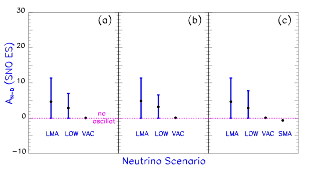
Figure 7: The percentage difference between the night and the day $\nu+e$ scattering rates. The figure shows the night-day percentage difference, i.e., $100\times A_{\rm N-D}({\rm SNO\;ES})$ defined in eq. (15). Predictions are shown for the solar neutrino oscillation scenarios allowed at $3\sigma$ and illustrated in figure 1. The three panels refer to results for different analysis strategies described in section 3. Figure 5 was constructed using a recoil electron kinetic energy threshold of $6.75$ MeV. Table 6 gives numerical results for $A_{\rm N-D}({\rm SNO\;ES})$ for kinetic energy thresholds of $4.5$ MeV and $6.75$ MeV.

Figure 7 and table 6 show the predicted (percentage) night-day differences for $\nu+e$ scattering in the SNO detector. The calculated values for $A_{\rm N-D}({\rm SNO~{}ES})$ were obtained using the $3\sigma$ boundaries of the global oscillation solutions shown in figure 1.

Table 6: The predicted $\nu+e$ Day-Night Asymmetry in SNO. The table presents $A_{\rm N-D}({\rm SNO~{}ES})$ in percent. The results are tabulated for different neutrino oscillation scenarios determined by our standard strategy and for two different thresholds of the recoil electron kinetic energy, $4.5$ MeV (columns two through four) and $6.75$ MeV (columns five through seven). The ranges are obtained for the 3$\sigma$ regions for figure 1(a).

	b.f.	max	min	b.f.	max	min
Scenario	4.5 MeV	4.5 MeV	4.5 MeV	6.75 MeV	6.75 MeV	6.75 MeV
	AN-D	AN-D	AN-D	AN-D	AN-D	AN-D
LMA	4.1	10.1	0.0	4.7	11.4	0.0
LOW	3.3	7.8	0.0	2.9	7.1	0.0
VAC	0.0	0.1	-0.1	0.1	0.3	-0.2

The values of $A_{\rm N-D}({\rm~{}ES})$ that are predicted for the Super-Kamiokande and the SNO locations are very similar. For the Super-Kamiokande location, the LMA solution, and a kinetic energy threshold of $4.5$ MeV ( corresponding to the recent Super-Kamiokande electron recoil energy threshold [5]), the predicted range of $A_{\rm N-D}({\rm SK\;ES})$ is between $0.0$% and $10.4$%, with a best-fit value of $4.3$% . Similarly for the LOW solution, the predicted range is between $0.0$% and $7.3$%, with a best-fit value of $3.1$%. The predicted values of $A_{\rm N-D}({\rm~{}ES})$ at both the SNO and the Super-Kamiokande locations are negligibly small for the VAC solution. Comparing with table 6, we see that the range of predicted values of $A_{\rm N-D}({\rm~{}ES})$ differs, between the SNO and Super-Kamiokande locations, by at most $7$% of the predicted range.

The predictions for SNO can be compared with the measured result reported by the Super-Kamiokande collaboration [5]

$$A_{\rm N-D}({\rm SK\;ES})~{}=~{}0.033\pm 0.022({\rm stat.})^{+0.013}_{-0.012}({\rm sys.}).$$ (16)

Not surprisingly, the best-fit predictions for the $\nu+e$ day-night scattering difference in the SNO detector implied by the global solutions shown in figure 1a are all rather close to the best-estimate value obtained by Super-Kamiokande. The SNO predictions are also bounded by the $3\sigma$ Super-Kamiokande limits, i.e., the predicted SNO values lie between $0$% and $11$%. Figure 7 shows that the LMA solution allows the largest values for $A_{\rm N-D}({\rm SNO~{}ES})$ and the VAC solution predicts no day-night difference in $\nu+e$ event rates.

The $1\sigma$ allowed range for $A_{\rm N-D}({\rm SNO~{}ES})$ is $4.7^{+2.7}_{-3.1}\;$% for $6.75$ MeV and $4.1^{+2.4}_{-2.8}\;$% for a $4.5$ MeV threshold, both for analysis strategy (a). The results for strategies (b) and (c) are very similar.

The “Before and After” predictions for $A_{\rm N-D}({\rm SNO~{}ES})$ are essentially the same, with only minor differences. That is to say, that the results do not depend significantly on the choice between the previously standard value of $S_{17}(0)$ [19] and the most recent and precise value of $S_{17}(0)$ [8].

4.3.2 Correlation between $A_{\rm N-D}({\rm SNO~{}CC})$ and $A_{\rm N-D}({\rm SNO~{}ES})$

Figure 8 shows the correlation between the predicted values for the day-night effect of the CC rate, $A_{\rm N-D}({\rm SNO~{}CC})$, and the day-night effect of the neutrino-electron scattering rate, $A_{\rm N-D}({\rm SNO~{}ES})$. The two day-night effects are essentially proportional to each other. The essential features of the correlation shown in figure 8 can be derived analytically, as we show in the following discussion.

The survival probability of electron neutrinos can be written as

$$P_{ee}=P_{D}-(1-2P_{c})\cdot\cos 2\theta_{S}\cdot f_{\rm reg},$$ (17)

where

$$P_{D}=\frac{1}{2}+\frac{1}{2}(1-2P_{c})\cdot\cos 2\theta_{S}\cdot\cos 2\theta$$ (18)

is the survival probability in the absence of the Earth–matter effect, i.e., during the day. Here $\theta_{S}$ is the matter mixing angle at the production point inside the Sun ($\theta_{S}=\frac{\pi}{2}$ when the production point occurs at much higher densities than the resonant point) , and $P_{c}$ is the level crossing probability which describes the non-adiabaticity of the conversion inside the Sun. The Earth regeneration factor, $f_{\rm reg}$, is defined as:

$$f_{\rm reg}\equiv P_{2e}-\sin^{2}\theta~{},$$ (19)

where $P_{2e}$ is the probability of the $\nu_{2}\rightarrow\nu_{e}$ conversion inside the Earth. In the absence of the Earth–matter effect we have $P_{2e}=\sin^{2}\theta$, so that $f_{\rm reg}=0$.

For both LMA and most of LOW region the adiabaticity condition is satisfied and we can take $P_{c}\simeq 0$. Furthermore in the LOW region and in the lower part of the LMA region one has $\cos 2\theta_{S}=-1$. With these approximations the probabilities take the form

$$P_{ee} = \sin^{2}\theta+f_{\rm reg}\;,$$ (20)

$$P_{D} = \sin^{2}\theta\;,$$ (21)

And the day-night asymmetry for CC events can be written as

$$A_{\rm N-D}({\rm SNO\;CC})=2\frac{\langle P_{ee}\rangle-\langle P_{D}\rangle}{\langle P_{ee}\rangle}=2\frac{\langle f_{\rm reg}\rangle}{\sin^{2}\theta+\langle f_{\rm reg}\rangle}$$ (22)

where we have denoted by $\langle\rangle$ the averaging over the neutrino spectrum, the interaction cross section, and the energy resolution.

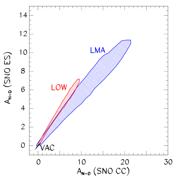
Figure 8: The correlation between the day-night effects for $\nu+e$ scattering and for CC events. The day-night effects shown in figure 5 and figure 7 are correlated for the standard analysis strategy that resulted in figure 1a. The predictions for the VAC solutions are essentially a point at the position (0,0).

The [ES] event rate is [ES] $\sim\langle P_{ee}+r(1-P_{ee})\rangle$ where $r\equiv\sigma_{\mu}/\sigma_{e}\simeq 0.15$ is the ratio of the the $\nu_{e}-e$ and $\nu_{\mu}-e$ elastic scattering cross-sections. Hence the day-night asymmetry for neutrino-electron scattering events can be written as

$$A_{\rm N-D}({\rm SNO\;ES})=2\frac{(1-r)\langle f_{\rm reg}\rangle}{\sin^{2}\theta+r\cos^{2}\theta+(1-r)\langle f_{\rm reg}\rangle}\;.$$ (23)

From eq. (22) and eq. (23), we see that the slope in the $A_{\rm N-D}({\rm SNO\;CC})$ versus $A_{\rm N-D}({\rm SNO\;ES})$ plot is given by

$$\frac{A_{\rm N-D}({\rm SNO\;ES})}{A_{\rm N-D}({\rm SNO\;CC})}=(1-r)\frac{\sin^{2}\theta+\langle f_{\rm reg}\rangle}{\sin^{2}\theta+r\cos^{2}\theta+(1-r)\langle f_{\rm reg}\rangle}\rightarrow(1-r)\frac{\sin^{2}\theta}{\sin^{2}\theta+r\cos^{2}\theta}$$ (24)

where the last implication applies in the region of small asymmetries. Using this relation and the ranges of mixing angles in the LOW and LMA solution we can reproduce the slope of the regions. From eq. (24), we see that the ratio of the asymmetries increases with the mixing angle and is larger for mixing angles on the dark side ($\theta>\pi/4$). Therefore eq. (24) explains why the LOW solution has a larger slope in figure 8 than the LMA solution.

4.4 CC recoil energy spectrum: first and second moments

Figure 9: The first moment: the fractional shift, $\delta T$, in percent for the average electron recoil energy. The figure shows the fractional change in percent for the average electron recoil energy, $\langle T\rangle$, relative to what is produced by an undistorted ${\rm{}^{8}B}$ neutrino energy spectrum. The predictions are shown at $3\sigma$ C.L. for the three different analysis strategies for neutrino oscillation solutions that are illustrated in figure 1. The calculations were performed assuming a $6.75$ MeV recoil electron kinetic energy threshold.

The solar influence on the shape of the ${\rm{}^{8}B}$ neutrino energy spectrum is only about one part in $10^{5}$ [44]. Therefore, in the absence of neutrino oscillations or other new physics, the energy spectrum of solar neutrinos incident on terrestrial detectors should be the same as the energy spectrum of ${\rm{}^{8}B}$ neutrinos produced in the laboratory. The incident solar neutrino energy spectrum can be studied well by observing the recoil energy spectrum of electrons produced by neutrino absorption (CC) reactions on deuterium, as shown in eq. (11). In the CC reaction, nearly all of the available kinetic energy is taken by the recoiling electron since the other particles in the final state are (massive) baryons.

The Super-Kamiokande experiment has already provided beautiful data on the recoil energy spectrum from neutrino electron scattering [5]. In recent publications by the Super-Kamiokande collaboration, these data are divided into $19$ separate energy bins. A number of authors have questioned whether using so many energy bins in a $\chi^{2}$ analysis of all the available data gives too much weight to the measurement of the spectral parameters(see, e. g., ref. [45] for a particularly insightful discussion of the statistical questions).

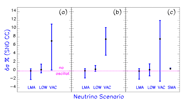
Figure 10: The second moment: the fractional shift, $\delta\sigma$, in percent for the standard deviation of the electron recoil energy spectrum. The figure shows the fractional change in the standard deviation of the electron recoil energy spectrum relative to what is expected for an undistorted ${\rm{}^{8}B}$ neutrino energy spectrum. The predictions are shown at $3\sigma$ C.L. for the three different analysis strategies for neutrino oscillation solutions that are illustrated in figure 1. The calculations were performed assuming a $6.75$ MeV recoil electron kinetic energy threshold.

In this subsection, we consider an alternative method of analysis of the SNO recoil energy spectrum in terms of small number of the lowest order moments of the distribution, a method that has been discussed in connection with solar neutrino experiments in refs. [35, 37, 46, 47]. We follow the notation and analysis of refs. [35, 46].

Figure 9 and figure 10 show the computed first and second moments of the recoil electron energy spectrum from the CC reaction, eq. (11), for the three different analysis strategies discussed in section 3 and illustrated in figure 1. These moments may well represent the essential physical content of the electron energy spectrum (cf. refs. [35, 46]) and could represent the results of the spectral measurements in a global oscillation analysis.

For both the first and second moments, the VAC solution predicts the largest deviation from the undistorted spectrum. Nevertheless, the range of predicted values is only about $\pm 2$% for the first moment and $\pm 7$% for the second moment. The non-statistical uncertainties in measuring the first and second moments in SNO have been estimated, prior to the operation of the experiment, in ref. [35] and are, respectively, about $1$% and $2$%.

Assuming the approximate validity of the prior estimate of the measuring uncertainties given in ref. [35], it seems very unlikely that SNO will determine a $3\sigma$ deviation from the undistorted spectrum if either the favored LMA or LOW oscillation solutions shown in figure 1 is correct. Although this is a negative prediction, it is nevertheless an important prediction. Even for the VAC solution, it will be very difficult to measure a significant deviation from an undistorted spectrum. The best opportunity to see a deviation will be in the second moment.

4.5 SNO: What if we are lucky?

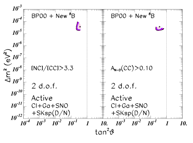
Figure 11: If nature is kind. The left panel shows the currently allowed regions for the neutrino oscillation parameters that predict a neutral current to charged current double ratio, [NC]/[CC], that is $>3.3$ and the right panel shows the currently allowed region that predicts a CC night-day difference, $A_{\rm N-D}({\rm SNO\;CC})$, that is $>0.1$. The calculations were performed assuming a $6.75$ MeV recoil electron kinetic energy threshold. The regions shown in figure 11 will change after measurements become available on either (or both) [NC]/[CC] or $A_{\rm N-D}({\rm SNO\;CC})$ and a new global solution is calculated.

Figure 3, figure 5, and table 5 show that if Nature has arranged things favorably, then only a rather small range of neutrino oscillation parameters can correctly predict the results. If SNO measures either a large value for the neutral current to charged current ratio, ${\rm[NC]/[CC]}>3.3$, or a large value for the night-day difference, $A_{\rm N-D}({\rm SNO\;CC})>0.1$, then the $\Delta m^{2}$ and $\tan^{2}\theta$ will be rather well determined.

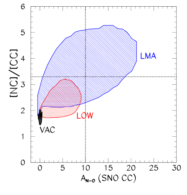
Figure 12: The correlation between the neutral current to charged current double ratio, [NC]/[CC], and the charged current day-night effect $A_{\rm N-D}({\rm SNO\;CC})$. The figure shows the allowed values at $3\sigma$ of [NC]/[CC] versus $100\times A_{\rm N-D}({\rm SNO\;CC})$, using the analysis strategy (a) and a CC threshold of $6.75$ MeV. The dotted lines show the limiting values $A_{\rm N-D}({\rm SNO\;CC})=10$% and [NC]/[CC] $=3.3$ used in figure 11.

Figure 11 shows the small range of neutrino parameters that, given the currently allowed regions defined by the currently available experimental data, can correctly predict the results if SNO shows that one of these inequalities is correct. In that fortunate situation, SNO will narrow down the allowed neutrino parameters to a small region in neutrino parameter space. With the currently available data, the boundaries of the region corresponding to ${\rm[NC]/[CC]}>3.3$ are for our standard analysis strategy, (a): $0.2<\tan^{2}\theta<0.4$ and $1.8\times 10^{-5}~{}{\rm eV^{2}}<\Delta m^{2}<1.0\times 10^{-4}~{}{\rm eV^{2}}$. For $A_{\rm N-D}>0.1$, the corresponding boundaries are $0.2<\tan^{2}\theta<0.7$ and $1.8\times 10^{-5}~{}{\rm eV^{2}}<\Delta m^{2}<3.5\times 10^{-5}~{}{\rm eV^{2}}$. The only change in the above numbers if we use the free ${\rm{}^{8}B}$ strategy (cf. figure 1c), rather than our standard analysis strategy is that the $A_{\rm N-D}$ range is slightly affected and the upper limit for $\Delta m^{2}$ decreases to $3.3\times 10^{-5}~{}{\rm eV^{2}}$.

The regions corresponding to ${\rm[NC]/[CC]}>3.3$ and $A_{\rm N-D}({\rm SNO\;CC})>0.1$ depend upon the data available when a global analysis is made. The regions shown in figure 11 will change after measurements become available on either (or both) [NC]/[CC] or $A_{\rm N-D}({\rm SNO\;CC})$ and a new global solution is carried out.

If bi-maximal mixing [30] is correct, one would not expect either ${\rm[NC]/[CC]}>3.3$ (this would be a $10\sigma$ deviation from predictions based upon existing experimental data, cf. figure 1) or $A_{\rm N-D}({\rm SNO\;CC})>0.1$ (a $3.8\sigma$ [$3.1\sigma$]deviation from the predictions of currently allowed solutions for analysis (a) [(c)]).

Figure 12 shows the correlation between the currently allowed values of [NC]/[CC] and $A_{\rm N-D}({\rm SNO\;CC})$. There is a general tendency that larger values of $A_{\rm N-D}\break({\rm SNO\;CC})$ are associated with larger values of [NC]/[CC], although the correlation is rather broad. For a given value of [NC]/[CC], a large range of values of$A_{\rm N-D}({\rm SNO\;CC})$ is currently allowed and vice-versa. Figure 12 also shows clearly that for smaller values of [NC]/[CC] and $A_{\rm N-D}({\rm SNO\;CC})$ discriminating among different oscillation scenarios will not be easy. For example, for the LMA solution, [NC]/[CC] $<2.1$ implies $A_{\rm N-D}({\rm SNO\;CC})<1$% . On the other hand, there is a range of neutrino parameters characterizing the LOW solution for which one expects ${\rm[NC]/[CC]}<2.1$ while there exists a small but non vanishing day-night asymmetry $1$% $<A_{\rm N-D}({\rm SNO\;CC})<8$%.

5 Predictions for ${\rm\bf{}^{7}Be}$ rate and day-night effect

In this section, we present the predictions of the globally allowed solutions for the neutrino electron scattering rate and the day-night effect in the BOREXINO [10] and KamLAND [11] detectors. For specificity, we present results for the location of BOREXINO, but comment in the text on the differences in the predictions for KamLAND and BOREXINO. We assume the same energy window for recoil electrons for both detectors, so the only cause for the differences in the predictions is the different latitude of the detector locations. In all cases, the differences are smaller than the expected measurement uncertainties.

We consider only electrons with recoil kinetic energies in the experimentally preferred range of $0.25~{}{\rm MeV}<T_{\rm e}<0.8~{}{\rm MeV}$ (cf. ref. [10]). For simplicity in presentation and following the general practice in the literature, we refer to these events as ${\rm{}^{7}Be}$ neutrino events. However, we include in our discussion neutrinos from all solar neutrino sources that produce recoil electrons in the indicated energy range. We make use of the predicted neutrino fluxes and uncertainties given by the BP00 standard solar model [12]. (The ${\rm{}^{8}B}$ neutrinos do not contribute significantly in this energy range.) The ${\rm{}^{13}N}$ and ${\rm{}^{15}O}$ neutrinos are, after ${\rm{}^{7}Be}$, the next most important neutrino sources for producing electrons with recoil kinetic energies between $0.25~{}{\rm MeV}$ and $0.8~{}{\rm MeV}$.

In order to indicate the insensitivity of our conclusions to the poorly known CNO neutrino fluxes, table 7 gives results for the scattering rate and the day-night difference both with and without including CNO and $pep$ neutrinos. The predicted values are insensitive to the non-${\rm{}^{7}Be}$ neutrinos, if their fluxes are comparable to the BP00 standard solar model fluxes.

We begin by discussing the $\nu-e$ scattering rate in section 5.1 and then discuss the day-night effect in section 5.2. The hypothetical accuracy with which KamLAND and BOREXINO may, together with previous solar neutrino experiments, determine neutrino oscillation parameters has been discussed in ref. [48].

5.1 ${\rm\bf{}^{7}Be}$ $\nu-e$ scattering rate

Figure 13 shows, for the currently allowed oscillation solutions, the expected $3\sigma$ range in BOREXINO of the reduced neutrino-electron scattering rate, $[{\rm{}^{7}Be}]$,

Table 7: ${\rm\bf{}^{7}Be}$: Neutrino-electron scattering rate and Day-Night Asymmetry. The table presents the reduced neutrino-electron scattering rate, [${\rm{}^{7}Be}$] (eq. 25), and the night-day difference, $A_{\rm N-D}$ (see, eq. 15 but the result is presented here in %), for recoil electrons with kinetic energies in the range $0.25~{}{\rm MeV}<T_{\rm e}<0.8~{}{\rm MeV}$. The numbers in parentheses were calculated assuming that only ${\rm{}^{7}Be}$ neutrinos contribute while the entries not in parentheses were obtained assuming the correctness of the BP00 standard solar model neutrino fluxes. The results are given for the three neutrino oscillation scenarios described in figure 1a. The ranges shown in the table correspond to the 3$\sigma$ allowed regions for figure 1a.

	b.f.	max	min	b.f.	max	min
Scenario	[R(7Be)]	[R(7Be)]	[R(7Be)]	AN-D	AN-D	AN-D
LMA	0.65(0.65)	0.76(0.76)	0.58(0.58)	0.0(0.0)	0.1(0.1)	0.0(0.0)
LOW	0.62(0.62)	0.74(0.74)	0.54(0.54)	27(27)	42(42)	0.0(0.0)
VAC	0.63(0.62)	0.79(0.78)	0.53(0.51)	-3.5(-3.8)	-1.1(-1.3)	-4.8(-5.3)

$$[{\rm{}^{7}Be}]~{}\equiv~{}\frac{\displaystyle{\sum_{i}\left[\int\phi_{i}(\nu_{e})\sigma_{i}(E,\nu_{e})+\int\phi_{i}(\nu_{x})\sigma_{i}(E,\nu_{x})\right]}}{\displaystyle\sum_{i}{\rm(Standard~{}Model~{}Value)_{i}}},~{}~{}0.25~{}{\rm MeV}<T_{\rm e}<0.8~{}{\rm MeV}.$$ (25)

The neutrino-electron scattering rate, $[{\rm{}^{7}Be}]$, is defined in eq. (25) as the ratio of the number of recoil electrons with kinetic energies in the range $0.25~{}{\rm MeV}<T_{\rm e}<0.8~{}{\rm MeV}$ divided by the number that is expected if the BP00 model is correct and there are no neutrino oscillations. The summation over the different neutrino sources $i$ includes all solar neutrino fluxes, although the $[{\rm{}^{7}Be}]$ neutrinos are expected to dominate according to the BP00 solar model. The $\mu$ and $\tau$ neutrinos are denoted by $\nu_{x}$ in eq. (25).

Figure 13 shows that all three of the analysis strategies described in section 3 yield rather similar predictions for the scattering rate.

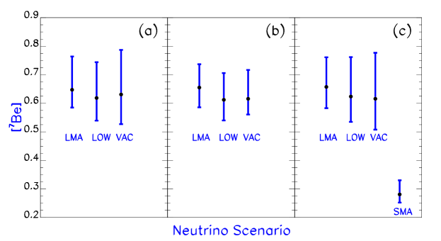
Figure 13: The ${\rm\bf{}^{7}Be}$ neutrino event rate. The figure shows [${\rm{}^{7}Be}$], the calculated $\nu_{e}+e^{-}$ event rate for all recoil electrons (including CNO neutrinos, see text) with kinetic energies in the range $0.25~{}{\rm MeV}<T_{\rm e}<0.8~{}{\rm MeV}$ relative to the rate that is expected for the BP00 standard model neutrino flux and no neutrino oscillations. The three panels of predictions in figure 13 were derived from the three panels of global solutions illustrated in figure 1 using the three analysis strategies described in section 3.

The predicted $3\sigma$ range of the neutrino electron scattering rate is (cf. table 7) $[{\rm{}^{7}Be}]=0.65^{+0.14}_{-0.12}$, where both the minimum value and the maximum value are achieved by vacuum solutions and the quoted limits correspond to our standard analysis strategy (cf. figure 1a). For the favored LMA solution, the range is somewhat smaller: $[{\rm{}^{7}Be}]=0.65^{+0.11}_{-0.07}$ (see also ref. [49]. The SMA solution, which is allowed at $3\sigma$ only in the “free ${\rm{}^{8}B}$ analysis strategy (cf. figure 1c), predicts much smaller values for $[{\rm{}^{7}Be}]$, namely, $[{\rm{}^{7}Be}]<0.34$ .

The $1\sigma$ predicted range is $[{\rm{}^{7}Be}]=0.65^{+0.04}_{-0.03}$ for our standard global analysis strategy (a). For the free ${\rm{}^{8}B}$ analysis strategy (c), the spread in predicted values of $[{\rm{}^{7}Be}]$ is somewhat larger, $[{\rm{}^{7}Be}]=0.66^{+0.05}_{-0.04}$. Analysis strategy (a) and (b) predict essentially the same $1\sigma$ range.

For KamLAND, the predicted range of $[{\rm{}^{7}Be}]$ is essentially the same as forBOREXINO. For the LMA and VAC solutions, the BOREXINO and KamLAND best-fit and maximum and minimum values are the same to three significant figures. For the LOW solution, the predicted range for KamLAND is about $1$% lower than for BOREXINO; the best-fit, maximum and minimum values are shifted downward for KamLAND.

5.2 ${\rm\bf{}^{7}Be}$ day-night variations

Figure 14 shows the predicted percentage difference between the night and the day rates that is expected for the BOREXINO experiment. As a number of previous authors have discussed (see, e. g., refs. [10, 50, 51] and references cited therein), the LOW solution is the only currently allowed oscillation solution that predicts a large night-day difference in the rates. The LMA solution predicts a negligible variation and therefore the $1\sigma$ predicted range is effectively zero.

The small night-day difference for the VAC solution shown in figure 14 and table 7 is the first calculation of this variation, with which we are familiar, for the low energies to which BOREXINO and KamLAND are sensitive. The physical origin of this variation has been described in section IXA of ref. [35]; it is due to the fact that the VAC survival probability depends upon the earth-sun separation and the longest nights occur in the Northern hemisphere when the earth-sun distance is shortest.

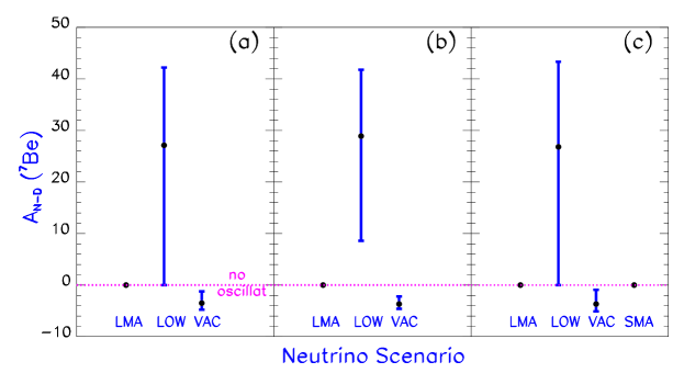
Figure 14: The percentage difference between the night and the day rates for recoil electrons with kinetic energies in the range $0.25~{}{\rm\bf MeV}<T_{\rm e}<0.8~{}{\rm\bf MeV}$. The figure shows the night-day percentage difference, i.e., $100\times A_{\rm N-D}$ defined in eq. (15). The predictions are given for the solar neutrino oscillation scenarios allowed at $3\sigma$ and illustrated in figure 1. The three panels refer to results for different analysis strategies described in section 3.

For KamLAND, the predicted range of values of $A_{\rm N-D}$ is very similar to the range predicted for BOREXINO. For the LMA solution, the predicted range of $A_{\rm N-D}$ for the two experiments is the same to an accuracy of better than $0.1$%. For the LOW solution, the maximum value for KamLAND is about $2$% less than for BOREXINO ($41$% compared to $42$%) and for the VAC solution, the minimum value is $-3.9$% for KamLAND compared to $-4.8$% for BOREXINO.

6 Predictions for KamLAND reactor experiment

The KamLAND detector [11, 52], located in the site of the famous Kamiokande experiment [53], consists of approximately one kton of liquid scintillator surrounded by photomultiplier tubes. KamLAND is sensitive to the $\bar{\nu}_{e}$ flux,

$$\bar{\nu_{e}}+p\to n+e^{+}\ ,$$ (26)

from 17 reactors that are located reasonably close to the detector. The distances from the different reactors to the experimental site vary from slightly more than 80 km to over 800 km, while the majority (roughly 80%) of the neutrinos travel from 140 km to 215 km (see, e.g., [52] for details).

KamLAND “sees” the antineutrinos by detecting the total energy deposited by recoil positrons, which are produced via reaction (26). The total visible energy, $E_{\rm visible}$, is

$$E_{\rm visible}~{}=~{}E_{e^{+}}~{}+~{}m_{e}~{}=~{}E_{\bar{\nu}}+m_{\rm p}-m_{\rm n}+m_{\rm e},$$ (27)

where $E_{e^{+}}$ is the total energy of the positron and $m_{\rm p},m_{\rm n}$,and $m_{e}$ are, respectively, the proton, neutron, and electron mass. The positron energy is related to the incoming antineutrino energy by $E_{e^{+}}=E_{\nu}-1.293$ MeV, up to small corrections related to the recoil momentum of the daughter neutron. KamLAND is expected to measure the visible energy with a resolution better than $\sigma(E)/E=10\%/\sqrt{E}$, for $E$ in MeV [52, 54].

Table 8: KamLAND event ratio and first and second visible energy moments. Here [CC] is the reduced charged current event ratio (defined below) and $\delta E_{\rm visible}$ and $\delta\sigma$ are the first two moments of the visible energy spectrum. The results are tabulated for two different thresholds of the visible energy, $1.22$ MeV (columns two through four) and $2.72$ MeV (columns five through seven). The ranges listed correspond to the 1 $\sigma$ and 3 $\sigma$ allowed regions for our standard LMA oscillation solution, (a).

	b.f.	max	min	b.f.	max	min
Scenario	1.22 MeV	1.22 MeV	1.22 MeV	2.72 MeV	2.72 MeV	2.72 MeV
		1 $\sigma$	1 $\sigma$		1 $\sigma$	1 $\sigma$
[CC]	0.44	0.66	0.37	0.39	0.68	0.33
$\delta E_{\rm visible}$ (%)	-5	+4	-10	+0.3	+4	-8
$\delta\sigma$ (%)	+8	+12	-15	+5	+6	-13
		3 $\sigma$	3 $\sigma$		3 $\sigma$	3 $\sigma$
[CC]	0.44	0.73	0.27	0.39	0.74	0.23
$\delta E_{\rm visible}$ (%)	-5	+9	-14	+0.3	+7	-11
$\delta\sigma$ (%)	+8	+18	-20	+5	+15	-18

In section 6.1 we present the predictions of the LMA solution (a) (cf. figure 1a) for the charged current capture rate (eq. 26) and for the distortion of the visible energy spectrum. We characterize the spectral distortion by the first and second moments of the energy distribution. No observable effect is predicted for the other currently allowed oscillation solutions. We describe in section 6.2 the calculational details of how the predictions were obtained.

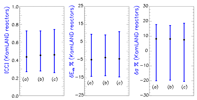
Figure 15: KamLAND reactor predictions. The figure shows the $3\sigma$ allowed predictions for the CC and the first and second moments of the visible energy spectrum relative to the expectations based upon the standard solar model and the standard electroweak model (cf. Table 8). The results are displayed for a visible energy threshold of $1.22$ MeV (cf. eqs. 29 and 30).

6.1 Predictions of global solution for charged current rate and spectrum distortion

Table 8 and Figure 15 summarize our principal predictions for the KamLAND reactor experiment.

The reduced charged current ratio, ${\rm[CC]}$, given in Table 8 is the ratio of the observed event rate for eq. (26) divided by the event rate predicted by the standard solar model (BP00) and the standard electroweak theory (no oscillations). Thus

$${\rm[CC]}~{}=~{}{{\rm(CC)_{Obs}\over(CC)_{SM}}}.$$ (28)

If the predictions of the standard solar model and the standard electroweak model are both correct, then ${\rm[CC]}~{}=~{}1.0$.

We find that the allowed range of the charged current ratio computed for a $1.2$ MeV total visible energy threshold and the LMA region shown in figure 1a is

$${\rm[CC]}~{}=~{}0.44^{+0.22}_{-0.07}(1\sigma)~{}~{}[0.44^{+0.29}_{-0.17}(3\sigma)],~{}~{}E_{\rm threshold}=1.22{\rm~{}MeV}.$$ (29)

For a somewhat higher visible energy threshold in which the background is less problematic (cf. refs. [54, 55, 56]), we find

$${\rm[CC]}~{}=~{}0.39^{+0.29}_{-0.06}(1\sigma)~{}~{}[0.39^{+0.35}_{-0.16}(3\sigma)],~{}~{}E_{\rm threshold}=2.72{\rm~{}MeV}.$$ (30)

Table 8 and Figure 15 represent the distortion of the visible energy spectrum by the fractional deviation from the undistorted spectrum of the first two moments of the energy spectrum (cf. the discussion in section 4.4) In the absence of oscillations, one expects $\langle E_{\rm vis}\rangle_{0}=3.97$ MeV and $\langle\sigma\rangle_{0}=1.26$ MeV for $E_{\rm threshold}=1.22$ MeV ($\langle E_{vis}\rangle_{0}=4.33$ MeV and $\langle\sigma\rangle_{0}=1.06$ MeV for $E_{\rm threshold}=1.72$ MeV). The predicted distortion of the energy spectrum, which can be as large as 20%, may be more difficult to measure than the predicted deviation from unity of the reduced charge current rate, [CC]. If a significant distortion of the spectrum is observed, the magnitude of the distortion will severely restrict the possible range of the oscillation parameters.

The results given here are in general agreement with other calculations that were made using previously determined allowed regions [11, 52, 54, 55, 56, 57, 48, 58, 59]. However, our calculations are the first that we know of that present the predicted distortions of the visible energy spectrum in terms of the first and second moments and which give the predicted values of the reduced charge current ratio for two separate energy thresholds (and for $1\sigma$ and $3\sigma$ deviations).

6.2 Calculational procedures and details

The antineutrino spectrum which is to be measured at KamLAND depends on the power output and fuel composition of each reactor (both change slightly as a function of time) and on the cross section for reaction (26). For the results presented here, we follow the flux and the cross section calculations and the statistical procedure described in ref. [55]. We define one “KamLAND-year” as the amount of time it takes KamLAND to observe $800$ events with visible energy above $1.22$ MeV. This is roughly what is expected after one year of running (assuming a fiducial volume of 1 kton), if all reactors run at (constant) $78\%$ of their maximal power output [52]. We assume a constant chemical composition for the fuel of all reactors (explicitly, 53.8% of ²³⁵U, 32.8% of ²³⁹Pu, 7.8% of ²³⁸U, and 5.6% of ²⁴¹Pu, see [59, 60]).

The shape of energy spectrum of the incoming neutrinos can be derived from a phenomenological parametrization, obtained in [61],

$$\frac{{\rm d}N_{\bar{\nu}_{e}}}{{\rm d}E_{\nu}}\propto e^{a_{0}+a_{1}E_{\nu}+a_{2}E^{2}_{\nu}},$$ (31)

where the coefficients $a_{i}$ depend on the parent nucleus. The values of $a_{i}$ for the different isotopes we used are tabulated in [61, 56]. These expressions are good approximations of the (measured) reactor flux for values of $E_{\nu}\gtrsim 2$ MeV.

The cross section for $\bar{\nu}_{e}+p\rightarrow e^{+}+n$ has been computed including corrections related to the recoil momentum of the daughter neutron in [62]. We used the hydrogen/carbon ratio, r=1.87, from the proposed chemical mixture (isoparaffin and pseudocumene) [52]. It should be noted that the energy spectrum of antineutrinos produced at nuclear reactors has been measured accurately in previous reactor neutrino experiments (see [52] for references). For this reason, we will assume for simplicity that the standard (without oscillations) antineutrino energy spectrum is known precisely. Some of the effects of uncertainties in the incoming flux on the determination of oscillation parameters have been studied in [56] and are estimated to be small.

The calculation is first done for visible energies $1.22<E_{vis}<7.22$ MeV and in the computation of the shifts on the visible energy moments we assume 12 energy bins (binwidth is 0.5 MeV). There still remains, however, the possibility of irreducible backgrounds from geological neutrinos in the lower energy bins ($E_{vis}\lesssim 2.6$ MeV) [54, 55, 56]. To verify how this possible background may affect the results we have repeated the analysis discarding the three lower energy bins i.e. considering only events with visible energies $2.72<E_{vis}<7.22$ MeV.

7 Discussion and summary

In this section, we summarize and discuss our principal results that are presented in the previous sections.

We summarize in section 7.1 our conclusions regarding solar model predictions and present in section 7.2 the currently allowed solar neutrino oscillation solutions that are found with three different analysis strategies. We describe the predictions of these allowed solutions for the SNO experiment in section 7.3 and for the BOREXINO and KamLAND experiments in section 7.4. In section 7.5 we discuss what can be learned from the BOREXINO and KamLAND solar neutrino experiments, despite the fact that the favored LMA, LOW, and VAC experiments all predict similar event rates. We describe the unique sensitivity of the reactor KamLAND experiment in section 7.6. Finally, we summarize in section 7.7 the robustness of the neutrino oscillation predictions and the possibilities for uniquely identifying the oscillation solution.

We present predictions for both $1\sigma$ and $3\sigma$ ranges of the currently allowed neutrino oscillation parameters.

We use the notation [Q] to represent the measured or predicted value of the quantity Q divided by the value expected for Q if one assumes the correctness of the standard solar model (BP00) and also assumes that nothing happens to the neutrinos after they are created in the sun.

7.1 Uncertainties in model predictions of solar neutrino fluxes

How does the ${\rm{}^{8}B}$ neutrino flux predicted by the solar model agree with the value inferred from the measurements by SNO [7] for the CC flux and by Super-Kamiokande [5] for the neutrino-electron scattering rate? Combining the SNO and Super-Kamiokande measurements, the SNO collaboration infers [7](see also [22, 63]) a total active ${\rm{}^{8}B}$ neutrino flux ($\nu_{e}+\nu_{\mu}+\nu_{\tau}$) of $\phi({\rm{}^{8}B;measured})=(5.44\pm 0.99)10^{6}{\rm~{}cm^{-2}s^{-1}}$. Comparing the measured ${\rm{}^{8}B}$ neutrino flux with the flux [12] calculated using the 1998 standard value for $S_{17}(0)$, $\phi({\rm{}^{8}B;BP00})=5.05(1^{+0.20}_{-0.16})10^{6}{\rm~{}cm^{-2}s^{-1}}$, one finds

$$\frac{\phi({\rm SNO+Super-Kamiokande})}{\phi({\rm BP00})}=1.08\pm 0.20({\rm measurement})\pm 0.18({\rm solar~{}model}).$$ (32)

Thus the measured flux agrees with the BP00 solar model flux to within $0.3\sigma$, combined experimental and theoretical errors. If we use instead the flux (see table 1) obtained with the more recent (Junghans et al.) value for $S_{17}(0)$, $5.93\times 10^{-4}\left(1.00^{+0.14}_{-0.15}\right)$, we find

$$\frac{\phi({\rm SNO+Super-Kamiokande})}{\phi({\rm BP00+New^{8}B})}=0.91\pm 0.17({\rm measurement})\pm 0.14({\rm solar~{}model}).$$ (33)

Therefore the measured flux agrees with the BP00 + ${\rm New^{8}B}$ solar model flux to within $0.4\sigma$, combined experimental and theoretical errors. In both cases, the measured and the solar model fluxes agree to better than $1\sigma$. The agreement between the predicted and measured ${\rm{}^{8}B}$ solar neutrino flux is a significant confirmation of the standard solar model since the rare ${\rm{}^{8}B}$ flux depends upon the $25$th power of the central solar temperature [64].

We present calculated results in this paper for two values of the crucial low energy cross section factor, $S_{17}(0)$, namely, $S_{17}(0)=19^{+4}_{-2}{\rm eVb}$ [19] (the 1998 standard value) and $S_{17}(0)=(22.3\pm 0.9){\rm eVb}$ [8] (the most recent and precise measurement). These two values of $S_{17}(0)$ represent well the range of measured cross section factors obtained in recent experiments [17]. The reader can therefore see at a glance the dependence of the calculated quantities upon the adopted value of the cross section $S_{17}(0)$.

Essentially all global analyses of solar neutrino oscillations make use of neutrino fluxes and their uncertainties obtained from a solar model. If the eight most important solar neutrino fluxes(cf. table 1 ) were allowed to vary without constraints, there would be too many free parameters to make possible an efficient study of solar neutrino oscillations. If the BP00 model is adopted in the analysis, then the total $p-p$ flux is assumed known to $\pm 1$% and the total ${\rm{}^{7}Be}$ flux is assumed known to $\pm 10$%.

Guidance from a solar model is required just to decide what are the most important neutrino fluxes to include in the analysis. For example, all current analyses of solar neutrino oscillations include a subset of the eight fluxes calculated in the standard solar model and listed in Table 1 but neglect the fluxes from the reactions $e^{-}+{\rm{}^{3}He}\rightarrow{\rm{}^{3}H}+\nu_{e}$,  $e^{-}+{\rm{}^{8}B}\rightarrow{\rm{}^{8}Be}+\nu_{e}$,  $e^{-}+{\rm{}^{13}N}\rightarrow{\rm{}^{13}C}+\nu_{e}$,  $e^{-}+^{15}{\rm O}\rightarrow{\rm{}^{15}N}+\nu_{e}$, and  $e^{-}+{\rm{}^{17}F}\rightarrow{\rm{}^{17}O}+\nu_{e}$. One must use the parameters of a solar model to show that the neglected fluxes are negligible [65] and that the included fluxes are important.

Even for a Bayesian analysis (see ref. [66]), one needs guidance from a solar model to determine which fluxes should be included and which should be neglected and, e. g., to decide if the priors should be expressed in terms of $10^{9}{\rm\,cm^{2}s^{-1}}$ for the ⁷Be flux and $10^{6}{\rm\,cm^{2}s^{-1}}$ for the ⁸B flux or vice versa. Nevertheless, the data for solar neutrino experiments is becoming sufficiently precise and constraining that Bayesian analyses can provide important and complimentary insights to results obtained with other statistical techniques (see, e.g., figure 20 of ref. [66]).

In a few cases, authors have carried out analyses in which the ${\rm{}^{8}B}$ neutrino flux, but none of the other fluxes, is completely unconstrained by the solar model predictions, which is our case (c) in section 3 and in figure 1c. The experimental data from solar neutrino experiments are not yet sufficient to permit a very restrictive analysis for unknown neutrino oscillation parameters if neutrino fluxes other than the ${\rm{}^{8}B}$ neutrino flux are allowed to be free variables.

The undesirable but currently unavoidable practice of using solar models to help constrain neutrino parameters is, ironically, the opposite practice to what was envisioned in the early days of solar neutrino research. The original chlorine experiment was proposed to test solar models using the assumed well-known properties of neutrinos [67].

In order to document what we use in this paper and to facilitate analyses of solar neutrino data by other groups, we summarize in section 2 the uncertainties and the best-estimates for solar neutrino fluxes derived from the BP00 solar model. We describe the results that are obtained when adopting the precise Junghans et al. value of $S_{17}(0)$ and also the results that are obtained using the 1998 standard value of $S_{17}(0)$(see especially table 1 and table 2 and related comments in the text).

We stress the continued importance of precise measurements of the low energy cross section factor, $S_{17}(0)$, for the ${\rm{}^{7}Be}$(p,$\gamma$)${\rm{}^{8}B}$ reaction. The neutrino fluxes measured in the Super-Kamiokande, SNO, and ICARUS solar neutrino experiments all depend linearly upon this cross section factor and the standard model prediction of the event rate in the chlorine experiment is also dominated by the ${\rm{}^{8}B}$ neutrino flux.

The uncertainty in the low energy cross section factor, $S_{34}(0)$, for the ${\rm{}^{3}He}$(${\rm{}^{4}He}$,$\gamma$) ${\rm{}^{7}Be}$ reaction dominates the uncertainty in the solar model calculation of the ${\rm{}^{7}Be}$ solar neutrino flux. The total uncertainty in the solar model calculation of the ${\rm{}^{7}Be}$ neutrino flux is $9$% and the ${\rm{}^{3}He}$(${\rm{}^{4}He}$,$\gamma$)${\rm{}^{7}Be}$ reaction contributes $8$% to the total uncertainty that is computed by quadratically combining uncertainties from different sources. The cross section factor $S_{34}(0)$ is also the largest nuclear physics uncertainty in the prediction of the ${\rm{}^{8}B}$ solar neutrino flux if one adopts the Junghans et al. value for the uncertainty in $S_{17}(0)$.

Now that there are precise measurements of $S_{17}(0)$ underway and completed, we believe the highest priority nuclear astrophysics measurement for the future is the precision determination of the low energy cross section factor for the ${\rm{}^{3}He}$(${\rm{}^{4}He}$,$\gamma$)${\rm{}^{7}Be}$ reaction. A measurement of $S_{34}(0)$ to an accuracy of better than $4$% is necessary in order to decrease the uncertainty in the reaction ${\rm{}^{3}He}$(${\rm{}^{4}He}$,$\gamma$)${\rm{}^{7}Be}$ to where it is no longer the largest uncertainty in the prediction of the ${\rm{}^{7}Be}$ solar neutrino flux.

7.2 Global neutrino oscillation solutions

Using three different analysis strategies that span the range of previously used strategies, we determine the globally allowed solar neutrino oscillation solutions that are consistent with all the available solar and reactor data. The results are summarized in figure 1; the calculations on which this figure is based used the new Junghans et al. value of $S_{17}(0)$. Table 3 gives the best-fit values of $\Delta m^{2}$ and $\tan^{2}\theta$, as well as the local value of $\chi^{2}_{\rm min}$ for each oscillation solution; the results presented in table 3 were obtained using our standard analysis strategy in which we take account of the BP00 + New ${\rm{}^{8}B}$ predicted fluxes and estimated uncertainties and include the Super-Kamiokande day and night energy spectrum but not the total rate. The $3\sigma$ upper limit to the allowed value of $\Delta m^{2}$ lies between $3.0$ and $7.5$, in units of $10^{-4}~{}{\rm eV^{2}}$, depending upon what is assumed about $S_{17}(0)$ and the analysis strategy.

The LMA solution is favored, but the LOW and VAC solutions are also allowed at a C.L. corresponding to $3\sigma$. Other solutions such as oscillations into sterile neutrinos or the SMA solution for active neutrinos are disfavored at $3\sigma$ if the standard analysis strategy is adopted, but SMA is barely allowed at $3\sigma$ if the ${\rm{}^{8}B}$ neutrino flux is unconstrained by the solar model predictions and uncertainties.

Figure 2 is a “Before and After” comparison of the effect of the ${\rm{}^{8}B}$ production cross section on the global oscillation solutions. The only difference between the “Before and After’ panels in figure 2 is the replacement in the analysis of the 1998 standard value of $S_{17}(0)=19^{+4}_{-2}{\rm eVb}$ [19] by the value obtained by the recent precise measurement, i.e., $S_{17}(0)=\left(22.3\pm 0.9\right){\rm eVb}$ [8]. Thus the “before” (left) panel of figure 2 corresponds to the results shown in the left panel of figure 9 of ref. [16]. The change in the value of $S_{17}(0)$ is sufficient to drive the SMA and Just So² solutions over the edge of the allowed region; they are allowed at $3\sigma$ with the older value of $S_{17}(0)$ but not with the newer value.

The global oscillation analysis yields a $3\sigma$ allowed range for the inferred total ${\rm{}^{8}B}$ solar neutrino flux expressed in terms of the best-estimate flux predicted by the BP00 model with the Junghans et al. value of $S_{17}(0)$. From table 4, we find for active neutrinos

$$0.40~{}\leq~{}f_{\rm B}~{}\leq~{}1.36,$$ (34)

for the case in which the ${\rm{}^{8}B}$ neutrino flux is unconstrained in the analysis. The best-fit value of $f_{\rm B}=1.0$ for this unconstrained case. The $3\sigma$ allowed range found here is slightly smaller than determined directly for active neutrinos by the SNO collaboration by comparing the SNO and Super-Kamiokande results. The SNO collaboration found [7] $f_{\rm B}=0.92\pm 0.50$, $3\sigma$ range. We show in section 3.2 that if one considers an arbitrary admixture of sterile and active neutrinos, the $3\sigma$ upper limit of $f_{\rm B}$ increases to $2.9$.

All of the global analyses of solar neutrino experiments that include the important Super-Kamiokande data [5] on the electron recoil energy spectrum use the many energy bins provided by the Super-Kamiokande group ($19$ energy bins in the last report). It would be very instructive to be able to carry out global analyses while representing the spectrum by only one or two measured quantities, the first or the first and second moments. One could then determine the change in the global solutions that result from giving the measurement of the energy spectrum the same prominence in the analysis as one or two measurements of the total rates.

Table 9: Neutrino oscillation predictions for the chlorine and gallium radiochemical experiments. The predictions are based upon the global analysis strategy (a), described in section 3, and make use of the neutrino fluxes given in table 1 for the BP00 solar model, the neutrino absorption cross sections given in ref. [20], and the Junghans et al. value of $S_{17}(0)$ [8]. The rates and $1\sigma$ uncertainties are presented for the best-fit values of the allowed solutions listed in table 3. The total rates should be compared with the standard solar model values of table 1, which are, $8.65^{+1.2}_{-1.1}$ (chlorine) and $130^{+9}_{-7}$(gallium), and the measured values, $2.56\pm 0.23$ (chlorine, see ref. [1])and $75.6\pm 4.8$(gallium, see ref. [2, 3, 4]).

Source	Cl	Ga	Cl	Ga	Cl	Ga
	(SNU)	(SNU)	(SNU)	(SNU)	(SNU)	(SNU)
	LMA	LMA	LOW	LOW	VAC	VAC
pp	0	41.8	0	38.7	0	44.3
pep	0.12	1.49	0.11	1.35	0.16	1.95
hep	0.01	0.02	0.02	0.03	0.03	0.04
${\rm{}^{7}Be}$	0.62	18.7	0.58	17.5	0.54	16.4
${\rm{}^{8}B}$	2.05	4.27	2.94	6.13	3.95	8.33
${\rm{}^{13}N}$	0.05	1.80	0.04	1.69	0.05	2.01
${\rm{}^{15}O}$	0.17	2.77	0.16	2.64	0.20	3.29
${\rm{}^{17}F}$	0.00	0.03	0.00	0.03	0.00	0.04
Total	$3.01\pm 0.31$	$71.0\pm 2.6$	$3.85\pm 0.45$	$68.1\pm 2.8$	$4.93\pm 0.60$	$76.4\pm 3.2$

We describe in Section 3.3 the technical differences between the three analysis strategies. This section is intended primarily for neutrino analysis junkies.

Table 9 presents the contributions of individual sources and the total rates predicted by the favored neutrino oscillation schemes, LMA, LOW, and VAC, for the chlorine and the gallium radiochemical experiments. The predictions are given in the table for our best-fit solutions obtained using the standard analysis strategy (a). The two measured rates are also listed. The errors are dominated by the solar model uncertainties for analysis strategy (a), which is apparent from table 9 by comparing the calculated and measured values. The theoretical uncertainties expressed in SNU for the chlorine and gallium rates are greatly reduced for the oscillation solutions (table 9) compared to the no-oscillation values (table 1). However, the theoretical uncertainties expressed as percentages of the total rates are comparable for the oscillation and no-oscillation scenarios.

All three of the oscillation scenarios yield total event rates in good agreement with the measured values for the gallium experiments. However, the calculated rates for the LOW and the VAC solutions are in poor agreement with the measured values (discrepancies of $2.7$ and $3.8$ $\sigma$, respectively). The global VAC solution is acceptable only because one can choose the ${\rm{}^{8}B}$ normalization such that the predicted distortion is small for the recoil energy spectrum measured by Super-Kamiokande. Of course, for strategy (c), in which the ${\rm{}^{8}B}$ neutrino flux is a free parameter, one can obtain global allowed solutions that are much better fits to the chlorine rate.

The predicted rates for the Super-Kamiokande experiment (in units of $\times 10^{6}\break{\rm cm^{-2}s^{-1}}$) are: $2.39^{+0.33}_{-0.36}$ (LMA), $3.02^{+0.42}_{-0.45}$ (LOW), and $3.81^{+0.53}_{-0.57}$(VAC), which should be compared with the measured rate of $(2.32\pm 0.03^{+0.08}_{-0.07})\times 10^{6}{\rm cm^{-2}s^{-1}}$ [5]. For the SNO CC measurement, the predicted rates are (in units of $\times 10^{6}{\rm cm^{-2}s^{-1}}$) : $1.72^{+0.24}_{-0.26}$ (LMA), $2.50^{+0.35}_{-0.38}$ (LOW), and $3.26^{+0.46}_{-0.49}$ (VAC), which should be compared with the measured rate of $(1.75\pm 0.07^{+0.12}_{-0.11})\times 10^{6}{\rm cm^{-2}s^{-1}}$ [7].

7.3 Predictions for SNO

All three analysis strategies yield essentially the same $3\sigma$ range for the neutral current to charged current double ratio(see figure 3) predicted by the favored LMA, LOW, and VAC solutions, namely, $1.4<{\rm[NC]/[CC]}<5.3$(For analysis strategy (c), with uses an unconstrained ${\rm{}^{8}B}$ neutrino flux, the upper limit extends to $6.2$.) The $1\sigma$ predicted range is $3.5\pm 0.6$ for our standard analysis strategy.

The predicted range of [NC]/[CC] for the favored oscillation solutions is also rather insensitive (see figure 4) to the choice of the ${\rm{}^{8}B}$ production cross section within the range of the 1998 standard value, ref. [19], and the recent precision determination, ref. [8]. If the ${\rm{}^{8}B}$ is allowed to vary freely, our analysis strategy (c), then the SMA solution for active neutrinos is allowed at the $3\sigma$ C.L. and for this solution $1.15<{\rm[NC]/[CC]}<1.31$. Figure 3 shows that all of the values of [NC]/[CC] predicted by the allowed neutrino oscillation solutions are separated from the no oscillation value of ${\rm[NC]/[CC]}=1.0$ by more than the expected experimental uncertainty.

For the average difference in the CC day-night effect, $A_{\rm N-D}({\rm SNO~{}CC})$, all three analysis strategies also yield essentially the same results, as is shown in figure 5. Figure 6 shows that the predictions for $A_{\rm N-D}({\rm SNO~{}CC})$ are also robust with respect to likely changes in the value of $S_{17}(0)$. The $3\sigma$ range in percent for all the oscillation solutions is $0.0\leq A_{\rm N-D}({\rm SNO~{}CC})\leq 0.21$ (The $1\sigma$ range is $A_{\rm N-D}({\rm SNO~{}CC})=8.15\pm 5.15\;$% .)

The predicted average difference in the day-night effect for neutrino-electron scattering, $A_{\rm N-D}({\rm SNO~{}ES})$, depends upon which among the currently allowed global oscillation solutions (LMA, LOW, VAC, or SMA) is assumed (see figure 7). All of the results are bounded by the $3\sigma$ allowed range for Super-Kamiokande, i. e., $A_{\rm N-D}({\rm SNO~{}ES})$ lies between $0$% and $11$%. Figure 8 shows the predicted correlation between the day-night effect for the CC and the day-night effect for neutrino-electron scattering. The predicted correlation between $A_{\rm N-D}({\rm SNO~{}ES})$ and $A_{\rm N-D}({\rm SNO~{}CC})$ constitutes an important consistency check for the oscillation solution.

The first and second moments of the electron recoil energy spectrum from CC reactions summarize most of the measurable information about the energy spectrum of ${\rm{}^{8}B}$ neutrinos that are observed by SNO (and by Super-Kamiokande). The low order moments may represent a more appropriate way to characterize the relatively undistorted energy spectrum rather than to provide event rates in a large number of separate spectral energy bins(cf. ref [5]). SNO has a significant advantage over Super-Kamiokande in measuring potential distortions of the energy spectrum due to neutrino oscillations, because the electron is the only light particle (hence it takes most of the energy) in the CC reaction, eq. (11).

The current set of allowed oscillation solutions do not predict distortions that are large enough to be detected by SNO at a high level of significance. Figure 9 and figure 10, when combined with the discussion in section 4.4 of the likely experimental uncertainties, establish this pessimistic prediction. Nevertheless, it is important to measure accurately the first two moments of the recoil energy distribution. The pessimistic prediction summarized here could be wrong if the correct oscillation solution is one not favored by the initial pioneering set of solar neutrino experiments (see further discussion of this point in section 7.7).

If we are lucky, if Nature is kind, then one measurement may define rather well the solar neutrino oscillation parameters. Figure 11 shows that only relatively small regions in neutrino oscillation parameter space predict that SNO will measure either ${\rm[NC]/[CC]}>3.3$ or $A_{\rm N-D}({\rm SNO\;CC})>0.1$, If either of these inequalities is established experimentally, then the oscillation parameters $\Delta m^{2}$ and $\tan^{2}\theta$ will be strongly constrained.

7.4 Solar neutrino predictions for BOREXINO and KamLAND

Table 7 and figure 13 show that the currently LMA, LOW, and VAC oscillation solutions predict similar values for the neutrino-electron scattering rate for ${\rm{}^{7}Be}$ neutrinos, $[{\rm{}^{7}Be}]=0.655\pm 0.035,1\sigma(0.66\pm 0.13,3\sigma)$. The SMA solution, which is allowed at $3\sigma$ only in the “free ${\rm{}^{8}B}$ analysis strategy (cf. figure 1c), predicts a much smaller value, ${[\rm^{7}Be]}<0.34$ .

Figure 14 and table 7 show that the LOW solution is the only currently allowed (at $3\sigma$) neutrino oscillation solution that predicts a significant day-night variability in BOREXINO or KamLAND. If a difference between day and night rates is actually observed, this will very strong evidence in favor of the LOW solution.

We have tested the robustness of the predictions for the BOREXINO and KamLAND experiment in several ways: i) we computed the predicted results for all three of the analysis strategies described in section 3; ii) we compared the results at the terrestrial locations of BOREXINO and KamLAND; and iii) we compared the predictions with and without including events from neutrino sources other than ${\rm{}^{7}Be}$. In all cases, the variations are small (and are given quantitatively in section 5).

How well can we predict $[{\rm{}^{7}Be}]$ if SNO measures either ${\rm[NC]/[CC]}>3.3$ or $A_{\rm N-D}({\rm SNO\>CC})>0.1$? Unfortunately, [${\rm{}^{7}Be}$] is not a unique function of the neutrino mixing parameters, $\Delta m^{2}$ and $\tan^{2}\theta$. Instead, [${\rm{}^{7}Be}$] can take on the same value for many different pairs of ($\Delta m^{2}$, $\tan^{2}\theta$). The predicted range of [${\rm{}^{7}Be}$] over the full LMA region allowed at $3\sigma$ is from $0.585$ to $0.76$. For the parameters corresponding to ${\rm[NC]/[CC]}>3.3$, the range is almost as large: $0.585$ to $0.74$. For $A_{\rm N-D}({\rm CC})>0.1$, the predicted range of [${\rm{}^{7}Be}$] is $0.585$ to $0.72$. Thus a hypothetical (and optimistic) experimental determination of the behavior of the survival probability, represented by figure 11, in the $6$ MeV to $10$ MeV region of neutrino energies most effectively probed by SNO would not be sufficient to allow a precise prediction of the survival probability at $0.86$ MeV, which corresponds to the energy of the ${\rm{}^{7}Be}$ neutrino line.

7.5 What will we learn from BOREXINO and KamLAND solar neutrino experiments?

At first impression, it may seem somewhat discouraging that the currently most favored oscillation solutions, LMA, LOW, and VAC, all predict very similar event rates for neutrino-electron scattering in BOREXINO and KamLAND (see figure 13). However, this is really an advantage.

If the currently favored oscillation solutions and the standard solar model are correct, then BOREXINO or KamLAND must confirm that $[{\rm{}^{7}Be}]=0.66\pm 0.13$. Thus the fact that the predicted event rates for BOREXINO and KamLAND are similar for the LMA, LOW, and VAC solutions means that a measurement of the neutrino electron scattering rate is a critical test of the validity of the standard solar model prediction and the favored oscillation solutions. In addition, we may be somewhat surprised and the measurements may show that $[{\rm{}^{7}Be}]<0.34$, favoring an SMA solution.

Also, a large measured value for the day-night effect in BOREXINO or KamLAND would imply the correctness of the LOW oscillation solution, which is currently allowed but is less favored than the LMA solution (cf. Table 3).

Experiments like BOREXINO and KamLAND that detect neutrinos with energies less than $1$ MeV are necessary to test the validity of solar neutrino oscillation solutions. The solutions explored in this paper, and in related papers by other authors, are primarily constrained by data that refer to the relatively high energies($>5$ MeV) for solar neutrinos to which the chlorine, Kamiokande, Super-Kamiokande and SNO experiments are primarily or exclusively sensitive. Of all the solar neutrino experiments performed so far, only the gallium experiments, SAGE and GALLEX + GNO, have a large sensitivity to low energy neutrinos. The gallium experiments are radiochemical experiments and therefore do not measure neutrino energies.

BOREXINO and KamLAND will also tell us something new and critical about the Sun. We have very little direct observational information about the important ${\rm{}^{7}Be}$ solar neutrino flux. If one supposes that ${\rm{}^{7}Be}$ is the only source contributing to the observed rates in the chlorine and gallium experiments, then the the $3\sigma$ upper limit implied by the chlorine measurements [1] is $2.8$ times the BP00 predicted flux. The upper limit implied by the gallium experiments [4, 2, 3] is $2.6$ times the BP00 predicted flux. All of the existing experiments are consistent with a ${\rm{}^{7}Be}$ flux that is identically zero. Thus the direct experimental constraints only require that

$$0.0~{}\leq~{}\frac{\phi(^{7}{\rm Be})}{\phi(^{7}{\rm Be})_{\rm BP00}}~{}\leq~{}2.6,~{}~{}3\sigma.$$ (35)

It is important to test experimentally whether the solar model prediction for the ${\rm{}^{7}Be}$ neutrino flux is correct. The branch of the $p-p$ fusion chain that is represented by ${\rm{}^{7}Be}$ neutrinos occurs in $15$% of the completions of the chain, according to the BP00 solar model.

In order to test the solar model prediction of the ${\rm{}^{7}Be}$ total neutrino flux, we must perform at least one additional experiment beyond the BOREXINO and KamLAND $\nu-e$ scattering experiments, which measure a linear combination of CC and NC events. Either a CC measurement or a NC measurement of the ${\rm{}^{7}Be}$ line is essential to test the solar model in a way that is completely free of all influence of solar models.

7.6 Predictions for the KamLAND reactor experiment

The KamLAND reactor experiment may provide definitive evidence for or against the LMA oscillation solution. The reduced charged current rate is predicted by the LMA solution to satisfy ${\rm[CC]}~{}=~{}0.44^{+0.22}_{-0.07}(1\sigma)~{}~{}[0.44^{+0.29}_{-0.17}(3\sigma)],~{}~{}E_{\rm threshold}=1.22{\rm~{}MeV}$, with a somewhat larger allowed range for a higher energy threshold. Table 8 summarizes the predicted distortion of the energy spectrum (in terms of the first and second moment) as well as the rate of the CC reaction for two plausible energy thresholds. If the LMA solution is correct, then the KamLAND experiment should observe a measurable deficit in the charged current rate. The spectral distortion, if measured, will determine the solar neutrino oscillation parameters with unprecedented precision.

7.7 Robustness and Uniqueness

The neutrino oscillation solutions that describe all the available solar and reactor data are, with one exception, robust with respect to variations among the three analysis strategies we have used in this paper. The SMA solution is the sole exception, and only just barely an exception. This solution exists at the $3\sigma$ C.L. if the ${\rm{}^{8}B}$ neutrino flux is treated as a free parameter (cf. figure 1), but the SMA is absent for all three analysis strategies at $99$% C.L.

The predictions for the quantities that are expected to be most easily measured by the SNO, BOREXINO, and KamLAND experiments are also robust with respect to analysis strategies.

If we are lucky, one of these experiments may determine uniquely the solar neutrino oscillation parameters. SNO could potentially identify the LMA solution as correct by observing a large value for either the neutral to charged current ratio or the day-night difference. KamLAND could also establish the LMA solution by finding an appreciable deficit of reactor antineutrinos in the first phase of the experiment. On the other hand, BOREXINO and KamLAND could definitively select the LOW solution if a large day-night effect is observed.

All of the above comments depend upon the validity of the global theoretical analysis which fits oscillation solutions to the reported results of the first six solar neutrino experiments: chlorine, Kamiokande, SAGE, GALLEX + GNO, Super-Kamiokande, and SNO. Because the analyses depend upon experimentally untested constraints implied by the standard solar model and because there is insufficient redundancy in the experiments performed so far, there may be startling surprises when solar neutrino oscillations are probed in the future in different experimental ways.

7.8 Late breaking news from Super-Kamiokande

The Super-Kamiokande collaboration has discussed [68] preliminary data for $1496$ days of observation, a $19$% increase in the length of data-taking over the previously reported data set of $1258$ days of observation. We are grateful to M. Smy for making the preliminary data available to us so that we could access the robustness of the predictions made in this paper to a modest amount of additional data.

Figure 16 shows the global solutions for the same three analysis strategies and input data as were used in producing figure 1, except that figure 16 makes use of $1496$ days of Super-Kamiokande data. At first glance, figure 1 and figure 16 are very similar to each other. With the new data, there is a small reduction in the lower-mass region of the LMA solution and in the upper-mass region of the LOW solution. The primary reasons for the changes that do occur are the somewhat smaller differences between the day and the night data and the slightly flatter (with respect to the undistorted standard spectrum) recoil energy spectrum. We spare the reader the details of the best-fit points (which are shown in figure 16) since these values bounce around within the allowed region as new data are obtained.

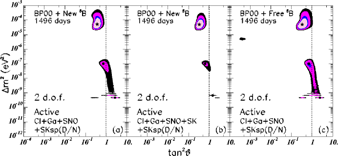
Figure 16: Global oscillation solutions including $1496$ days of Super-Kamiokande observations. Figure 16 is the same as figure 1 except that data from $1496$ days of Super-Kamiokande observations were used in constructing figure 16 whereas $1258$ days of Super-Kamiokande observations were used in constructing figure 1.

At what CL is LMA the unique solution to the solar neutrino data? In the global solution (strategy a) represented in figure 1, which includes 1258 days of Super-Kamiokande data, LMA is the only solution at $96$% ($2\sigma$) CL and in figure 16, for $1496$ days of Super-Kamiokande observations, LMA is the only solution at $97$% ($2.1\sigma$) CL. Even before the availability of the SNO data, LMA was the only solution at $86$% ($1.5\sigma$) CL [69]. These results are in good agreement with those described by Smy [68] (who analyzed the Super-Kamiokande data with more zenith-angle bins and fewer spectral energy bins than we do). We conclude that LMA is the preferred solution with a CL that has been increasing slowly with time.

Table 10 presents the $1\sigma$ and $3\sigma$ ranges for the principal solar neutrino observables that were calculated in sections 3-6. In constructing table 10, we again use analysis strategy (a) and the same input data as in the previous calculations except that we now include $1496$ days of Super-Kamiokande data.It is instructive to compare the entries in table 10 with the previously tabulated results. The changes due to the new data are smaller than or comparable to the differences among the predictions of the three analysis strategies for the total event rates and the energy shifts, i. e., for the quantities [NC]/[CC], $\delta$T(SNO CC), [⁷Be], [CC] (KamLAND), and $\delta E_{\rm vis}$ (KamLAND). We conclude, once again, that these predictions are robust.

The predicted maximum value at $3\sigma$ of the day-night asymmetry is reduced by about $15$% for the CC measurement by SNO (from $21$% to $18$%) and by about $10$% for BOREXINO (from $41$% to $38$%). These changes reflect the difficulty in measuring day-night asymmetries, which are determined by relatively small differences between two large numbers.

Table 10: Predictions including $1496$ days of Super-Kamiokande data. This table presents the $1\sigma$ and $3\sigma$ ranges for the measurable quantities calculated in sections 3-6. We use here analysis strategy (a) and the same input data as in the previous calculations, except that $1496$ days of Super-Kamiokande data were included. Results are presented for measurables in the SNO, BOREXINO, and KamLAND experiments. The threshold of the recoil electron kinetic energy used in computing the SNO observables for this table is $6.75$ MeV and for the KamLAND reactor observables, $E_{\rm th}=1.22$ MeV. The recoil energy range for the BOREXINO experiment is the same as adopted in section 5.

Observable	b.f. $\pm 1\sigma$	b.f. $\pm 3\sigma$
$[$NC$]/[$CC$]$	$3.41^{+0.64}_{-0.50}$	$3.41^{+1.64}_{-2.00}$
AN-D(SNO CC)	$5.1^{+5.5}_{-3.1}$	$5.1^{+12.9}_{-5.4}$
AN-D(SNO ES)	$2.9^{+2.9}_{-1.7}$	$2.9^{+6.7}_{-3.1}$
$\delta$T% (SNO CC)	$0.00^{+0.02}_{-0.36}$	$0.00^{+1.53}_{-1.33}$
$[$R(7Be)$]$	$0.66\pm 0.03$	$0.66^{+0.13}_{-0.11}$
AN-D(7Be)	—	$23^{+15}_{-28}$
$[$CC$]$(KamLAND)	$0.56^{+0.11}_{-0.16}$	$0.56^{+0.17}_{-0.27}$
$\delta E_{\rm visible}$(KamLAND) (%)	$-7^{+11}_{-3}$	$-7^{+15}_{-7}$

We are grateful to E. G. Adelberger and K. A. Snover for discussions of their important new measurement of the ${\rm{}^{7}Be+p}$ cross section and to V. Barger, S. Glashow, D. Marfatia, A. McDonald, M. Smy, R. Svoboda, and J. Wilkerson for valuable comments and discussions. A. Piepke made the very useful suggestion that we include predictions for the KamLAND reactor experiment and M. Chen and A. McDonald drew our attention to the relation between the day-night effects in SNO of the CC and the neutrino-electron scattering. JNB acknowledges support from NSF grant No. PHY0070928. MCG-G is supported by the European Union Marie-Curie fellowship HPMF-CT-2000-00516. This work was also supported by the Spanish DGICYT under grants PB98-0693 and PB97-1261, by the Generalitat Valenciana under grant GV99-3-1-01, and by the ESF network 86.

References

- [1] B.T. Cleveland et al., Measurement of the solar electron neutrino flux with the Homestake chlorine detector, Astrophys. J. 496 (1998) 505.
- [2] W. Hampel et al. (GALLEX Collaboration), GALLEX solar neutrino observations: results for GALLEX IV, Phys. Lett. B 447 (1999) 127.
- [3] M. Altmann et al. (GNO Collaboration), GNO solar neutrino observations: results for GNO I, Phys. Lett. B 490 (2000) 16; E. Bellotti et al. (GNO Collaboration), First results from GNO, in Neutrino 2000, Proc. of the XIXth International Conference on Neutrino Physics and Astrophysics, 16–21 June 2000, eds. J. Law, R.W. Ollerhead, and J.J. Simpson, Nucl. Phys. B 91 (Proc. Suppl.) (2001) 44.
- [4] J.N. Abdurashitov et al. (SAGE Collaboration), Measurement of the solar neutrino capture rate with gallium metal, Phys. Rev. C 60 (1999) 055801 [astro-ph/9907113]; V. Gavrin (SAGE Collaboration), Solar neutrino results from SAGE, in Neutrino 2000, Proc. of the XIXth International Conference on Neutrino Physics and Astrophysics, 16–21 June 2000, eds. J. Law, R.W. Ollerhead, and J.J. Simpson, Nucl. Phys. B 91 (Proc. Suppl.) (2001) 36.
- [5] Y. Fukuda et al. (Super-Kamiokande Collaboration), Measurements of the solar neutrino flux from Super-Kamiokande’s first 300 days, Phys. Rev. Lett. 81 (1998) 1158; Erratum 81 (1998) 4279; Constraints on neutrino oscillation parameters from the measurement of day-night solar neutrino fluxes at Super-Kamiokande, Phys. Rev. Lett. 82 (1999) 1810; Y. Suzuki (Super-Kamiokande Collaboration), Solar neutrino results from Super-Kamiokande, in Neutrino 2000, Proc. of the XIXth International Conference on Neutrino Physics and Astrophysics, 16–21 June 2000, eds. J. Law, R.W. Ollerhead, and J.J. Simpson, Nucl. Phys. B 91 (Proc. Suppl.) (2001) 29; S. Fukuda et al. (Super-Kamiokande Collaboration), Solar and hep neutrino measurements from 1258 days of Super-Kamiokande data, Phys. Rev. Lett. 86 (2001) 5651.
- [6] M. Apollonio et al., Limits on neutrino oscillations from the CHOOZ experiment, Phys. Lett. B 466 (1999) 415.
- [7] Q.R. Ahmad et al., Measurement of charged current interactions produced by solar neutrinos at the Sudbury Neutrino Observatory, Phys. Rev. Lett. 87 (2001) 071301.
- [8] A.R. Junghans et al., astrophysical S-factor from precision cross section measurements, Phys. Rev. Lett. 88 (2002) 041101.
- [9] A.B. McDonald (SNO collaboration), The Sudbury Neutrino Observatory project, Nucl. Phys. B 77 (Proc. Suppl.) (1999) 43; G.T. Ewan, W.F. Davidson, C.K. Hargrove (SNO Collaboration), The Sudbury Neutrino Observatory—an introduction, Physics in Canada 48 (1992) 112; SNO Collaboration, The Sudbury Neutrino Observatory, Nucl. Instrum. Meth. A 449 (2000) 172.
- [10] G. Alimonti et al. (BOREXINO collaboration), Science and Technology of BOREXINO: a real time detector for low energy solar neutrinos, Astropart. Phys. 16 (2002) 205.
- [11] P. Alivisatos et al. (the KamLAND collaboration), KamLAND: a liquid scintillator anti-neutrino detector at the Kamioka site, Stanford-HEP-98-03; A. Piepke (KamLAND Collaboration), KamLAND: a reactor neutrino experiment testing the solar neutrino anomaly, in Neutrino 2000, Proc. of the XIXth International Conference on Neutrino Physics and Astrophysics, 16–21 June 2000, eds. J. Law, R.W. Ollerhead, and J.J. Simpson, Nucl. Phys. B 91 (Proc. Suppl.) (2001) 99.
- [12] J.N. Bahcall, M.H. Pinsonneault, S. Basu, Solar models: current epoch and time dependences, neutrinos, and helioseismological properties, Astrophys. J. 555 (2001) 990.
- [13] J.N. Bahcall, P.I. Krastev, A.Yu. Smirnov, Solar neutrinos: global analysis and implications for SNO, JHEP 0105(2001)015 [hep-ph/0103179].
- [14] M.C. Gonzalez-Garcia, M. Maltoni, C. Peña-Garay, J.W.F. Valle, Global three-neutrino oscillation analysis of neutrino data, Phys. Rev. D 63 (2001) 033005 [hep-ph/0009350].
- [15] J.N. Bahcall, P.I. Krastev, A.Yu. Smirnov, Where do we stand with solar neutrino Oscillations?, Phys. Rev. D 58 (1998) 096016.
- [16] J.N. Bahcall, M.C. Gonzalez-Garcia, Carlos Peña-Garay, Global analysis of solar neutrino oscillations including SNO CC measurement, JHEP 08(2001)014.
- [17] R.W. Kavanagh, T.A. Tombrello, J.M. Mosher, D.R. Goosman, The cross section, Bull. Am. Phys. Soc. 14 (1969) 1209; P.D. Parker, reaction, Phys. Rev. 150 (1966) 851; F.J. Vaughn, R.A. Chalmers, D. Kohler, L.F. Chase, Jr., Cross sections for the reaction, Phys. Rev. C 2 (1970) 1657; C. Wiezorek, H. Kräwinkel, R. Santo, L. Wallek, Study of the -reaction, Zeits. fur Physik A 282 (1977) 121; B.W. Filippone, A.J. Elwyn, C.N. Davids, D.D. Koetke, Proton capture cross section of and the flux of high energy solar neutrinos, Phys. Rev. C 28 (1983) 2222; F. Hammache et al., New measurement and analysis of the cross section, Phys. Rev. Lett. 80 (1998) 928; F. Hammache et al., Low energy measurement of the cross section, Phys. Rev. Lett. 86 (2001) 3985; L. Gialanella et al., Absolute cross section of using a novel approach, European Phys. J. A 7 (2000) 303; F. Strieder et al., Absolute cross section of , Nucl. Phys. A 696 (1-2) (2001) 219; M. Hass et al., A new measurement of the cross-section with an implanted target, Phys. Lett. B 462 (1999) 237; B. Davids et al., determined from the Coulomb breakup of 83 MeV/nucleon , Phys. Rev. Lett. 86 (2001) 2750.
- [18] J.N. Bahcall, Neutrino Astrophysics, Cambridge University Press, Cambridge 1989.
- [19] E.C. Adelberger et al., Solar Fusion Cross Sections, Rev. Mod. Phys. 70 (1998) 1265.
- [20] J.N. Bahcall, Gallium solar neutrino experiments: absorption cross sections, neutrino spectra, and predicted event rates, Phys Rev C 56 (1997) 3391; J.N. Bahcall et al., Standard neutrino spectrum from decay, Phys. Rev. C 54 (1996) 411.
- [21] P.I. Krastev and A.Yu. Smirnov, Global analysis with SNO: toward the solution of the solar neutrino problem, accepted for publication in Phys. Rev. D [hep-ph/0108177].
- [22] G.L. Fogli, E. Lisi, D. Montanino, A. Palazzo, Model-dependent and independent implications of the first Sudbury Neutrino Observatory results, Phys. Rev. D 64 (2001) 093007.
- [23] J.N. Bahcall, S. Basu, M.H. Pinsonneault, How uncertain are solar neutrino predictions?, Phys. Lett. B 433 (1998) 1.
- [24] A.V. Gruzinov and J.N. Bahcall, The electron capture rate in the sun, Astrophys. J. 490 (1997) 437 [astro-ph/9702065].
- [25] V. Barger, D. Marfatia, K. Whisnant, Unknowns after the SNO charged-current measurement, Phys. Rev. Lett. 88 (2002) 011302; V. Barger, D. Marfatia, K. Whisnant, Piecing the Solar Neutrino Puzzle Together at SNO, Phys. Lett. B 509 (2001) 19.
- [26] M.V. Garzelli and C. Giunti, Bayesian view of solar neutrino oscillations, JHEP 12(2001)017.
- [27] A. Bandyopadhyay, S. Choubey, S. Goswami, K. Kar, Impact of the first SNO results on neutrino mass and mixing, Phys. Lett. B 519 (2001) 83; A. Bandyopadhyay, S. Choubey, S. Goswami, K. Kar, Three generation neutrino oscillation parameters after SNO [hep-ph/0110307].
- [28] G.L. Fogli, E. Lisi, D. Montanino, Matter-enhanced three-flavor oscillations and the solar neutrino problem, Phys. Rev. D 54 (1996) 2048.
- [29] A. Gouvea, A. Friedland, H. Murayama, The dark side of the solar neutrino parameter space, Phys. Lett. B 490 (2000) 125.
- [30] H. Minakata and O. Yasuda, Constraining almost degenerate three-flavor neutrinos, Phys. Rev. D 56 (1997) 1692; A. Yu. Smirnov, Lepton mixing: small, large, maximal? [hep-ph/9907296]; H. Georgi and S.L. Glashow, Neutrinos on earth and in the heavens, Phys. Rev. D 61 (2000) 097301; K. Choi, E.J. Chun, K. Hwang, W.Y. Song, Bi-maximal neutrino mixing and small from Abelian flavor symmetry, Phys. Rev. D 64 (2001) 113013; A. Ghosal, Two parameter texture of nearly bimaximal neutrino mixing, Phys. Rev. D 62 (2000) 092001; Q. Shafi and Z. Tavartkiladze, Anomalous flavor (1): predictive texture for bi-maximal neutrino mixing, Phys. Lett. B 482 (2000) 145; R.N. Mohapatra, A. Pérez-Lorenzana, C.A. de S. Pires, Type II seesaw and a gauge model for the bimaximal mixing explanation of neutrino puzzles, Phys. Lett. B 474 (2000) 355; V. Barger, S. Pakvasa, T.J. Weiler, K. Whisnant, Bi-maximal mixing of three neutrinos, Phys. Lett. B 437 (1998) 107; C.S. Kim and J.D. Kim, Hierarchical quark mixing and bimaximal lepton mixing on the same footing, Phys. Rev. D 61 (2000) 057302; A. Baltz, A.S. Goldhaber, M. Goldhaber, An oscillation solution with maximal neutrino mixing, Phys. Rev. Lett. 81 (1998) 5730; M. Jeżabek and Y. Sumino, Neutrino mixing and see-saw mechanism, Phys. Lett B 440 (1998) 327; G. Altarelli and F. Feruglio, Neutrino mass textures from oscillations with maximal mixing, Phys. Lett. B 439 (1998) 112; Z.-z. Xing, Bimaximal neutrino mixing pattern reexamined, Phys. Rev. D 61 (2000) 057301; P.H. Frampton and S.L. Glashow, Can the Zee ansatz for neutrino masses be correct?, Phys. Lett. B 461 (1999) 95; Y. Koide and A. Ghosal, Bimaximal neutrino mixing in a Zee-type model with badly broken flavor symmetry, Phys. Rev. D 63 (2001) 037301; W.G. Scott, Tri-maximal vs. bi-maximal neutrino mixing, Nucl. Phys. B 85 (Proc. Suppl.) (2000) 177; Y.-L. Wu, Spontaneous breaking of flavor symmetry and naturalness of nearly degenerate neutrino masses and bi-maximal mixing, Sci. China A 43 (2000) 988.
- [31] R. S. Raghavan, Solar neutrinos: from puzzle to paradox, Science 267 (1995) 45; P. I. Krastev and S. T. Petcov, On the vacuum oscillation solution of the solar neutrino problem, Phys. Rev. D 53 (1996) 1665.
- [32] M.C. Gonzalez-Garcia and C. Peña-Garay, Four-neutrino oscillations at SNO, Phys. Rev. D 63 (2001) 073013.
- [33] G.L. Fogli and E. Lisi, Standard solar model uncertainties and their correlations in the analysis of the solar neutrino problem, Astropart. Phys. 3 (1995) 185 with updated uncertainties as discussed in G.L. Fogli, E. Lisi, D. Montanino, A. Palazzo, Three-flavor MSW solutions of the solar neutrino problem, Phys. Rev. D 62 (2000) 013002.
- [34] J.N. Bahcall, P. Krastev, A.Yu. Smirnov, What will the first year of SNO show?, Phys. Lett. B 477 (2000) 401.
- [35] J.N. Bahcall, P.I. Krastev, A.Yu. Smirnov, SNO: predictions for ten measurable quantities, Phys. Rev. D 63 (2000) 093004.
- [36] J.N. Bahcall and P.I. Krastev, How well do we (and will we) know solar neutrino fluxes and oscillation parameters?, Phys. Rev. D 53 (1996) 4211.
- [37] J.N. Bahcall and E. Lisi, Tests of electron flavor conservation with the Sudbury Neutrino Observatory, Phys. Rev. D 54 (1996) 5417.
- [38] S. Ying, W.C. Haxton, E.M. Henley, Charged- and neutral-current cross sections for heavy-water Cherenkov detectors, Phys. Rev. C 45 (1992) 1982.
- [39] S. Nakamura, T. Sato, V. Gudkov, K. Kubodera, Neutrino reactions on the deuteron, Phys. Rev. C 63 (2001) 034617.
- [40] M. Butler, J.-W. Chen, X. Kong, Neutrino-deuteron scattering in effective field theory at next-to-next-to-leading order, Phys. Rev. C 63 (2001) 035501.
- [41] S.P. Mikheyev and A.Yu. Smirnov, Neutrino oscillations in matter with varying density, in ’86 Massive Neutrinos in Astrophysics and in Particle Physics, proceedings of the Sixth Moriond Workshop, eds. O. Fackler and Y. Trân Thanh Vân, Editions Frontières, Gif-sur-Yvette 1986, p. 355; M. Cribier, W. Hampel, J. Rich, D. Vignaud, MSW regeneration of solar electron-neutrino in the earth, Phys. Lett. B 182 (1986) 89; A.J. Baltz and J. Weneser, Effect of transmission through the earth on neutrino oscillations, Phys. Rev. D 35 (1987) 528; S. Hiroi, H. Sakuma, T. Yanagida, M. Yoshimura, An effective lower bound of the solar neutrino flux, Phys. Lett. B 198 (1987) 403; A. Dar, A. Mann, Y. Melina, D. Zajfman, Neutrino oscillations and the solar-neutrino problem, Phys. Rev. D 35 (1988) 3607; M. Spiro and D. Vignaud, Solar model independent neutrino oscillation signals in the forthcoming solar neutrino experiments?, Phys. Lett. B 242 (1990) 279; N. Hata and P. Langacker, Earth effect in the MSW analysis of the solar neutrino experiments, Phys. Rev. D 48 (1993) 2937; J.N. Bahcall and P.I. Krastev, Does the sun appear brighter at night in neutrinos?, Phys. Rev. C 56 (1997) 2839; J.M. Gelb, W. Kwong, S.P. Rosen, Searching for the Mikheyev-Smirnov-Wolfenstein enhancement, Phys. Rev. Lett. 78 (1997) 2296; E. Lisi and D. Montanino, Earth regeneration effect in solar neutrino oscillations: an analytic approach, Phys. Rev. D 56 (1997) 1792; M. Maris and S.T. Petcov, Study of the day-night effect for the Super-Kamiokande detector. II. Electron spectrum deformations and day-night asymmetries, Phys. Rev. D 56 (1997) 7444; M. Maris and S.T. Petcov, Day-night effect predictions for the SNO detector, Phys. Rev. D 62 (2000) 093006; A.H. Guth, L. Randall, M. Serna, Day-night and energy dependence of MSW solar neutrinos for maximal mixing, JHEP 08(1999)018; V. Barger, D. Marfatia, K. Whisnant, B. P. Wood, Earth regeneration of solar neutrinos at SNO and Super-Kamiokande, Phys. Rev. D 64 (2001) 073009; G.L. Fogli, E. Lisi, D. Montanino, A. Palazzo, Quasivacuum solar neutrino oscillations, Phys. Rev. D 62 (2000) 113004; M. Maris and S. Petcov, Day-night effect predictions for the SNO detector, Phys. Rev. D 62 (2000) 093006.
- [42] M.C. Gonzalez-Garcia, C. Pena-Garay, A.Yu. Smirnov, Zenith angle distributions at Super-Kamiokande and SNO and the solution of the solar neutrino problem, Phys. Rev. D 63 (2001) 113004 [hep-ph/0012313].
- [43] J. N. Bahcall, P. Krastev, A. Yu. Smirnov, Correlations of solar neutrino observables for SNO, Phys. Rev. D 63 (2001) 053012.
- [44] J.N. Bahcall, Shapes of solar-neutrino spectra: unconventional tests of the standard electroweak model, Phys. Rev. D 44 (1991) 1644.
- [45] P. Creminelli, G. Signorelli, A. Strumia, Frequentist analyses of solar neutrino data, JHEP 05(20001)052 [hep-ph/0102234].
- [46] J.N. Bahcall, P.I. Krastev, E. Lisi, Neutrino oscillations and moments of electron spectra, Phys. Rev. D 55 (1997) 494.
- [47] G. Fiorentini, M. Lissia, G. Mezzorani, M. Moretti, D. Vignaud, Solar neutrino experiments and determination of the neutrino oscillation parameters, Phys. Rev. D 49 (1994) 6298; W. Kwong and S.P. Rosen, Method for analyzing electron spectra observed in solar neutrino experiments, Phys. Rev. D 51 (1995) 6159; see also Energy dependence of solar-neutrino-electron scattering as a test of neutral currents, Phys. Rev. Lett. 68 (1992) 748.
- [48] A. Strumia and F. Vissani, Which solar neutrino experiment after KamLAND and BOREXINO?, JHEP 11(2001)048.
- [49] S.M. Bilenky, T. Lachenmaier, W. Potzel, F. von Feilitzsch, Implications of the SNO and the Homestake results for the BOREXINO experiment [hep-ph/0109200].
- [50] A. de Gouvea, A. Friedland, H. Murayama, Earth matter effect in solar neutrino experiments, JHEP 0103(2001)009.
- [51] J. Bahcall and P.I. Krastev, Does the sun appear brighter at night in neutrinos?, Phys. Rev. C 56 (1997) 2839.
-
[52]
J. Busenitz et al.,
Proposal for US participation
in KamLAND, March 1999 (unpublished). May be downloaded from
http://bfk0.lbl.gov/kamland/. - [53] Y. Fukuda et al. (Kamiokande Collaboration), Solar neutrino data covering solar cycle 22, Phys. Rev. Lett. 77 (1996) 1683.
-
[54]
K. Ishihara (KamLAND Collaboration), The
current status of KamLAND,
talk given at the NuFACT’01 Workshop in Tsukuba, Japan (May 24–30, 2001).
Transparencies at
http://psux1.kek.jp/~nufact01/index.html. - [55] A. de Gouvea and C. Pena-Garay, Solving the solar neutrino puzzle with KamLAND and solar data, Phys. Rev. D 64 (2001) 113011.
- [56] H. Murayama and A. Pierce, Energy spectra of reactor neutrinos at KamLAND, Phys. Rev. D 65 (2002) 013012.
- [57] R. Barbieri and A. Strumia, Non standard analysis of the solar neutrino anomaly, JHEP 0012(2000)016.
- [58] M.C. Gonzalez-Garcia and C. Pena-Garay, On the effect of on the determination of solar oscillation parameters at KamLAND, Phys. Lett. B 527 (2002) 199.
- [59] V. Barger, D. Marfatia, B.P. Wood, Resolving the solar neutrino problem with KamLAND, Phys. Lett. B 498 (2001) 53.
- [60] Y. Declais et al., Study of reactor anti-neutrino interaction with proton at Bugey Nuclear Power Plant, Phys. Lett. B 338 (1995) 383.
- [61] P. Vogel and J. Engel, Neutrino electromagnetic form-factors, Phys. Rev. D 39 (1989) 3378.
- [62] P. Vogel and J.F. Beacom, The angular distribution of the reaction , Phys. Rev. D 60 (1999) 053003.
- [63] G.L. Fogli, E. Lisi, A. Palazzo, F.L. Villante, Solar neutrino event spectra: tuning SNO to equalize Super-Kamiokande, Phys. Rev. D 63 (2001) 113016 [hep-ph/0102288]; F.L. Villante, G. Fiorentini, E. Lisi, Solar neutrino interactions: using charged currents at SNO to tell neutral currents at Super-Kamiokande, Phys. Rev. D 59 (1999) 013006 [hep-ph/9807360]; C. Giunti, Are there or in the flux of solar neutrinos on Earth?, Phys. Rev. D 65 (2002) 033006; V. Berezinsky, Exact analysis of the combined data of SNO and Super-Kamiokande [hep-ph/0108166].
- [64] J.N. Bahcall and A. Ulmer, Temperature dependence of solar neutrino fluxes, Phys. Rev. D 53 (1996) 4202.
- [65] J.N. Bahcall, Line versus continuum solar neutrinos, Phys. Rev. D 41 (10) (1990) 2964.
- [66] M.V. Garzelli and C. Giunti, Model independent information on solar neutrino oscillations [hep-ph/0111254].
- [67] J.N. Bahcall, Solar neutrinos. I. Theoretical, Phys. Rev. Lett. 12 (1964) 300; R. Davis Jr. Solar neutrinos. II. Experimental, Phys. Rev. Lett. 12 (1964) 303.
- [68] M.B. Smy, A unique oscillation solution to the solar neutrino problem?, talk at the 3rd Workshop on Neutrino Oscillations and Their Origin (NOON2001), December 5–8, 2001, Kashiwa, Japan [hep-ex/0202020].
- [69] M.C. Gonzalez-Garcia, M. Maltoni and C. Pena-Garay, Solar and atmospheric four-neutrino oscillations, Phys. Rev. D 64 (2001) 093001.