Hadronic potentials from effective field theories

Abstract

We construct the potentials that describe the spectrum and decay of electromagnetic bound states of hadrons, and are consistent with ChPT. These potentials satisfy the matching condition which enables one to express the parameters of the potential through the threshold scattering amplitudes calculated in ChPT. We further analyze the ambiguity in the choice of the short-range hadronic potentials, which satisfy this matching condition.

I Introduction

The energy spectrum and decays of electromagnetic bound states of strongly interacting particles - so called hadronic atoms - have recently been measured by several experimental collaborations. These measurements yield an extremely valuable piece of information about the behavior of QCD at a very low energy, which is hardly accessible with a different experimental technique. In particular, the measurement of the $\pi^{+}\pi^{-}$ atom decay width by DIRAC collaboration at CERN [1] which will result in the determination of the difference $a_{0}-a_{2}$ of the $S$-wave $\pi\pi$ scattering lengths at a $5\,\%$ precision, would allow one to directly test the large/small condensate scenario of chiral symmetry breaking in QCD with two flavors. Further, the Pionic Hydrogen collaboration at PSI intends to extract the $S$-wave $\pi N$ scattering lengths from the ongoing measurement of the spectrum and transition energies between $3p-1s$ levels in pionic hydrogen at a $1\,\%$ accuracy which is unique in hadron physics [2]. This will yield a more precise value of the $\pi NN$ coupling constant and of the $\pi N$ $\sigma$-term. Finally, the DEAR collaboration [3] at the DA$\Phi$NE facility plans to measure the energy level shift and lifetime of the $1s$ state in $K^{-}p$ and $K^{-}d$ atoms - with considerably higher precision than in the previous experiment carried out at KEK [4] for $K^{-}p$ atoms. It is expected [3] that this will result in an accurate determination of the $I=0,1$ $S$-wave scattering lengths. It will be a challenge for theorists to extract from this new information on the $\bar{K}N$ amplitude at threshold a more precise value of e.g. the $KN$ $\sigma$-term and of the strangeness content of the nucleon.

In order to fully exploit the high-precision experimental data, it is imperative to design the theoretical framework for the analysis of these data which would describe this sort of bound states in the accuracy that matches the experimental precision. In practice, this would mean that the Deser-type formulae [5] which are used to extract the strong scattering lengths from the measured values of the energy shift and width of hadronic atoms, do not provide the necessary precision and should be corrected to accommodate strong and electromagnetic isospin-breaking corrections which typically amount up to a few percent. Since these corrections arise in a result of a complicated interplay of strong and electromagnetic effects in the bound-state observables, some dynamical input on strong interactions is needed for their evaluation. Starting from [6], the problem of the calculation of hadronic atom observables has been analyzed within the potential scattering theory approach (see, e.g. [7, 8, 9, 10]), where the strong interactions are described by the short-range “hadronic” potentials. In order to possess a predictive power, certain assumptions about the strong potential should be made within this approach - it is usually assumed that the short-range strong potential does not violate the isospin symmetry and describes purely hadronic data at low energy. Isospin-breaking corrections are then calculated by taking into account the kinematical effect due to the mass difference of charged and neutral particles, including Coulomb interaction, vacuum polarization and some higher-order pure QED effects.

The issue of “purification” of the experimental data with respect to strong and electromagnetic isospin-breaking corrections arises in the context of the the low-energy hadronic scattering processes as well. This problem is closely related to the problem of the hadronic bound states, which were discussed above. Two distinct approaches are available in the literature to address the issue in the scattering sector: the dispersion relations approach [11, 12], and the potential scattering theory approach (see, e.g. [13, 14, 15]). The results obtained within these two approaches are used e.g. in the recent analysis of the low-energy $\pi N$ scattering data [12, 16].

Recently, the problem of isospin-breaking corrections in hadronic atom observables has been addressed in the framework of ChPT [17, 18, 19, 20, 21, 22] (see Ref. [20] for the comparison of different approaches). In a result of these investigations, a systematic discrepancy between the results obtained within the potential scattering theory approach and the field-theoretical approach, has been discovered for the case of the $\pi^{+}\pi^{-}$ atom decay width and the $\pi^{-}p$ atom ground-state energy. In particular, the prediction for the $\pi^{+}\pi^{-}$ atom decay width [7, 8, 9] depends on the potential used, and on the choice of the free Green function in the Schrödinger equation. Earlier calculations [7] have predicted the isospin-breaking corrections with the opposite sign and with the same order of magnitude as in ChPT. In the later paper [8], including some kinematic relativistic corrections in the free Green function, the authors obtain a result for the lifetime $\tau=3.0\times 10^{-15}~{}sec$ which is still not compatible with the existing prediction of ChPT: for a fixed value of $a_{0}-a_{2}$, the lifetime equals to $\tau=2.9\times 10^{-15}~{}sec$ with an accuracy of $1.2\,\%$ [22]. The latest prediction of the potential model for the lifetime is numerically close to that of ChPT [9]. However, no compelling physical reasons are available in favor of the conclusion, that the latest version includes all relevant isospin-breaking corrections from the underlying theory. The potential-approach based prediction for the energy shift of the $\pi^{-}p$ atom [10] differs by a factor $2$ from the order-of magnitude estimate carried out in ChPT at $O(p^{2})$ [21], and quotes the value $0.5\,\%$ for the systematic error which is $4$ times smaller than the corresponding value obtained from ChPT. Even if the values of the low-energy constants (LECs) in ChPT turn out to be such (see Ref. [23] for the evaluation of these constants in the quark model), that the prediction for the correction in ChPT comes numerically close to that of the potential approach, still the systematic error is underestimated in the potential approach. Of course, the large systematic error in the prediction of ChPT comes from the LECs which, albeit poorly known in the $\pi N$ case, are still present and can not be simply disregarded. In addition, we would like to stress here that there is no physical reason why the LECs in ChPT must have the particular values which reproduce the results of the potential approach.

The discrepancy mentioned above does not come to a surprise: the potential which is used to calculate the bound-state observables, does not include a full content of isospin-breaking effects in QCD+QED. It has been demonstrated (see, e.g. [24]) that the isospin-symmetric short-range potential which has been used so far, can not fully accommodate the effect of the direct quark-photon interaction, as well as the isospin-breaking effect due to the explicit dependence of the scattering amplitude on the quark masses which is governed by the chiral symmetry. These effects turn out to be dominant in the isospin-breaking part of $\pi\pi$ and $\pi N$ interactions at threshold, that leads to the above-mentioned discrepancy. Moreover, since the potential approach makes use of the same ideology in the calculation of the isospin-breaking corrections to hadronic scattering amplitudes in the low-energy region, the same criticism is applicable in this case as well - in fact, a significant discrepancy between the results of the potential approach and those of the ChPT in the analysis of $\pi N$ scattering process has already been reported [25].

The aim of the present paper is to explicitly demonstrate, how the potential model can be made compatible with ChPT - in what concerns the calculation of the isospin-breaking corrections to the observables of hadronic atoms. This construction will help one to finally resolve the long-standing puzzle and to determine the status of the potential approach-based calculations in the analysis of the hadronic atom data. Moreover, in the view of the fact that the potential approach is widely used to evaluate the isospin-breaking effects in scattering processes, it is important to note that the same construction allows one to constrain the potential from comparing the threshold amplitudes in the field theory and in the potential approach. In this vein, one may hope to reduce the ambiguity in the prediction of the isospin-breaking corrections above threshold. The ultimate goal of our investigation is to derive the short-range hadronic potentials - including the part which violates the isospin symmetry - from ChPT. Although extensive investigations address the similar issue in the context of purely strong potential (see, e.g. [26, 27, 28]), to the best of our knowledge, the comprehensive study of isospin-breaking effects is not available in the literature.

The layout of the present paper is follows. In Section II we briefly review the derivation of the potential in the absence of isospin breaking. Section III deals with the simplified case of one-channel scattering, whereas in Section IV we address the inclusion of the isospin-breaking effects in full generality (multichannel scattering, relativistic corrections). In Section V we compare the results obtained within ChPT and existing potential models. Finally, Section VI contains our conclusions.

II Strong potential

For demonstrative purposes, below we shall briefly review the basic idea which lies in the foundation of the present approach. Assume that one starts from a given relativistic field theory, and is aimed at the construction of the potential which, used in the Lippmann-Schwinger equation, produces the same $S$-matrix elements at low energies, as the initial relativistic field theory. In order to achieve this goal, it has proven very useful, at an intermediate stage, to construct the non-relativistic effective field theory that correctly describes the low-energy behavior of the initial relativistic theory. To ease the consideration, we treat here the simplest case of scalar self-interacting field. Electromagnetic effects are assumed to be absent. In the low-energy domain (at energies much less than the mass of the particle), the physics can be described on the basis of the non-relativistic Lagrangian

$${\cal L}=\phi^{\dagger}\biggl{(}i\partial_{t}-M+\frac{\triangle}{2M}+\frac{\triangle^{2}}{8M^{3}}+\cdots\biggr{)}\phi+g_{0}(\phi^{\dagger}\phi)^{2}+g_{1}\phi^{\dagger}\phi^{\dagger}\stackrel{{\scriptstyle\leftrightarrow}}{{\triangle}}\phi\phi+g_{2}\phi^{\dagger}\phi\stackrel{{\scriptstyle\leftrightarrow}}{{\triangle}}\phi^{\dagger}\phi+\,,\cdots$$ (2.1)

where $M$ is the physical mass of the particle, $u\stackrel{{\scriptstyle\leftrightarrow}}{{\triangle}}v\doteq u(\triangle v)+(\triangle u)v$, and $\phi(x)$ is the non-relativistic field operator

$$\phi(0,{\bf x})=\int d\nu({\bf p})\,{\rm e}^{i{\bf p}{\bf x}}\,{\bf a}({\bf p})\,,\quad\quad[{\bf a}({\bf p}),{\bf a}^{\dagger}({\bf k})]=(2\pi)^{3}\delta^{3}({\bf p}-{\bf k})\,,\quad\quad d\nu({\bf p})\doteq\frac{d^{3}{\bf p}}{(2\pi)^{3}}\,.$$ (2.3)

The Lagrangian (2.1) contains an infinite string of local operators with an increasing mass dimension, which describe the scattering process $\phi\phi\rightarrow\phi\phi$. The operators which contain powers of space derivatives are suppressed by the corresponding power of $M$ which is the only heavy scale available. Thus, the contribution of these operators becomes increasingly suppressed at a small momenta $|{\bf p}|<<M$. Note that higher orders in time derivative $\partial_{t}$ can be systematically eliminated by the use of the equations of motion, without altering the $S$-matrix elements (see, e.g. [29]).

The detailed discussion of the perturbation theory based on the Lagrangian (2.1) can be found in Refs. [22, 29] - below, we only provide the sketch of the procedure. The $S$-matrix element for the scattering process in the non-relativistic theory is given by a sum of tree diagrams, plus any number of $s$-channel bubbles, plus mass insertions in the external and internal lines which come from the higher-order terms in the kinetic part of the Lagrangian (see Fig. 1). The free propagator of the scalar field is given by

$$i\langle 0|T\bar{\phi}(x)\bar{\phi}^{\dagger}(0)|0\rangle=\int\frac{d^{4}p}{(2\pi)^{4}}\,\frac{1}{M+{\bf p}^{2}/(2M)-p^{0}-i\epsilon}\,,$$ (2.4)

where $\bar{\phi}$ denotes the free field. To ease notation, we omit $-i\epsilon$ term in the following. The elementary building block in the calculation of the diagram with any number of strong bubbles in the CM frame is given by

$$J(P^{0})=\int\frac{d^{D}l}{(2\pi)^{D}i}\,\frac{1}{M+{\bf l}^{2}/(2M)-P^{0}+l^{0}}\,\frac{1}{M+{\bf l}^{2}/(2M)-l^{0}}\,=\frac{iM}{4\pi}\,(M(P^{0}-2M))^{1/2}$$ (2.5)

at $D\rightarrow 4,\,\,P^{0}>2M$. The scattering matrix elements are obtained by putting $P^{0}=2w({\bf p})$ where $w({\bf p})=(M^{2}+{\bf p}^{2})^{1/2}$ is the energy of the particle in the CM frame. At threshold, in dimensional regularization, the integral is purely imaginary and is proportional to $i|{\bf p}|$ where ${\bf p}$ is the three-momentum of the particle in the CM frame. The integrals containing derivative vertices and/or mass insertions can be considered analogously. According to the standard power-counting, their contribution will be suppressed by the corresponding power of $|{\bf p}|$.

The matching condition for the relativistic $T^{R}$ and non-relativistic $T^{NR}$ scattering amplitudes in the CM frame reads

$$T^{R}({\bf p},{\bf q})=4w^{2}({\bf p})\,T^{NR}({\bf p},{\bf q})\,,\quad\quad|{\bf p}|=|{\bf q}|\,.$$ (2.7)

This matching condition is understood as follows. At threshold, both relativistic and non-relativistic amplitudes can be expanded in powers of CM momenta ${\bf p}$ and ${\bf q}$

$$T^{I}=f_{0}^{I}+|{\bf p}|f_{1}^{I}+{\bf p}^{2}f_{2}^{I}+{\bf p}{\bf q}\,f_{3}^{I}+O({\bf p}^{3})\,,\quad\quad I=R,NR\,.$$ (2.8)

The matching condition then gives the relation between the coefficients of the expansion in the left and right-hand sides of Eq. (2.7). In the lowest order in ${\bf p}$, the non-relativistic scattering amplitude is completely determined by the tree diagram containing the coupling $g_{0}$ (Fig. 1a) - bubbles, derivative vertices and mass insertions all give the contributions that vanish at threshold. Consequently, the matching condition in the lowest order in ${\bf p}$ reads

$$4M^{2}\,(2!)^{2}\,g_{0}=T^{R}({\bf 0},{\bf 0})\,,$$ (2.9)

where in the right-hand side the $S$-wave scattering length in the relativistic theory appears (here $2!$ is the symmetry factor for the identical particles in the initial and final states). Note that in the matching, we have not used the perturbative expansion in the relativistic theory, so the above relation is valid “in any order in strong coupling constant”. Further, using the same technique, the coupling $g_{1}$ can be related to the $S$-wave effective radius and the $S$-wave scattering length, the coupling $g_{2}$ can be related to the $P$-wave scattering length, and so on.

In the following discussion, we shall first neglect derivative couplings, as well as mass insertions ${\bf p}^{4}/(8M^{3})\cdots$. These will be considered in Section IV. The non-relativistic scattering amplitude in this case is given by

$$T^{NR}({\bf p},{\bf q})=\frac{4g_{0}}{1-\frac{ig_{0}M}{2\pi}|{\bf p}|}\,.$$ (2.10)

Now it is straightforward to check that all strong bubbles with non-derivative vertex $g_{0}$ can be resummed with the help of the following Lippmann-Schwinger equation

$$T(E;{\bf p},{\bf q})=V({\bf p},{\bf q})+\frac{1}{2!}\,\int\frac{d^{d}{\bf l}}{(2\pi)^{d}}\,V({\bf p},{\bf l})\,\frac{1}{E-{\bf l}^{2}/M}\,T(E;{\bf l},{\bf q})\,,$$ (2.11)

and

$$({\bf q}|T(E)|{\bf p})\biggr{|}_{|{\bf q}|=|{\bf p}|,~{}E={\bf q}^{2}/M}=-\,T^{NR}({\bf q},{\bf p})\biggr{|}_{|{\bf q}|=|{\bf p}|}\,,$$ (2.12)

where $V({\bf p},{\bf q})=-(2!)^{2}\,g_{0}$, and we have used dimensional regularization to regulate UV divergences in physical dimensions $d\rightarrow 3$. Note that the operator $T(E)$ acts in the Hilbert space of vectors $|{\bf p})$, whereas $T^{NR}({\bf p},{\bf q})$ are the matrix elements of the scattering operator $T^{NR}$ in the Fock space between two-particle states $|{\bf p},-{\bf p}\rangle={\bf a}^{\dagger}({\bf p}){\bf a}^{\dagger}(-{\bf p})|0\rangle$, with the CM momentum removed (for details, see [19, 22]). Below, to ease discussion, we shall not explicitly distinguish between the state vectors in the two spaces.

Now we address our main task of deriving the potential from initial relativistic field theory. In principle, Eq. (2.11) already solves this problem - in the dimensional regularization. The potential has then a $\delta$-type singularity in the coordinate space

$$V({\bf r},{\bf r}^{\prime})=\int\frac{d^{d}{\bf p}}{(2\pi)^{d}}\,\frac{d^{d}{\bf q}}{(2\pi)^{d}}\,{\rm e}^{i{\bf p}{\bf r}-i{\bf q}{\bf r}^{\prime}}\,V({\bf p},{\bf q})=-(2!)^{2}\,g_{0}\,\delta^{d}({\bf r}-{\bf r}^{\prime})\,\delta^{d}({\bf r})\,.$$ (2.13)

In the conventional scattering theory it is customary to deal, however, not with the pointlike interactions in the dimensional regularization, but rather with the smooth potentials in the position space in the physical space dimensions $d=3$. We may accommodate this feature by smoothing the potential which is obtained from field theory, and simultaneously adjusting the coupling $g_{0}$ so that the scattering amplitude still obeys the matching condition (2.9). We demonstrate this procedure for the simplest case when one assumes the separable ansatz for the resulting potential

$$V({\bf r},{\bf r}^{\prime})\rightarrow V_{\beta}({\bf r},{\bf r}^{\prime})=-(2!)^{2}\,g_{0}(\beta)\,v({\bf r})\,v({\bf r}^{\prime})\,,\quad\quad v({\bf r})=\frac{\beta^{2}{\rm e}^{-\beta r}}{4\pi r}\,,\quad v({\bf p})=\frac{\beta^{2}}{\beta^{2}+{\bf p}^{2}}\,,$$ (2.14)

where $g_{0}(\beta)$ stands for the potential strength, and $\beta$ is the potential range parameter (we anticipate that, in a result of matching, $g_{0}(\beta)$ will depend on $\beta$). The scattering amplitude in the case of the separable interaction is given by

$$T(E;{\bf p},{\bf q})=-(2!)^{2}\,g_{0}(\beta)\,v({\bf p})\,v({\bf q})\,\biggl{[}1+2!\,g_{0}(\beta)\,\int\frac{d^{3}{\bf l}}{(2\pi)^{3}}\,\frac{v^{2}({\bf l})}{E-{\bf l}^{2}/M}\biggr{]}^{-1}\,.$$ (2.15)

The matching condition for the scattering amplitude at threshold then gives

$$4M^{2}\,(2!)^{2}\,g_{0}(\beta)=\frac{T^{R}({\bf 0},{\bf 0})}{1+\frac{\beta}{64\pi M}\,T^{R}({\bf 0},{\bf 0})}\,.$$ (2.16)

Of course the choice of the separable ansatz is not unique - one may, e.g. use the local ansatz $V({\bf r},{\bf r}^{\prime})\rightarrow\delta^{3}({\bf r}-{\bf r}^{\prime})\,V_{\beta}({\bf r})$ where $\beta$ denotes a range parameter for the potential. One may further choose any form for the potential $V_{\beta}({\bf r})$, e.g. use the double square well potential [7]. In the absence of the analytic solution in this case one will have to solve the matching condition for the coupling constant numerically. The generalization to higher-order terms in ${\bf p}^{2}$ expansion, as well as for higher partial waves is straightforward.

To summarize, we note that, according to the point of view adopted through the present paper, the smooth potentials in the position space are nothing than a particular regularization of the genuine pointlike interactions between particles, which stem from the underlying field theory. The shape of the potential thus bears no important physical information. The physical input from the underlying theory is contained in the couplings, and enters through the matching condition, which states that the fixed number of terms in the effective-range expansion of the scattering matrix elements coincide in the potential approach and in the underlying relativistic field theory. This is enough for both approaches to describe the same physics in the vicinity of the scattering threshold.

III Isospin-breaking effects in the one-channel case

In this section, we discuss the inclusion of the electromagnetic effects in the scheme considered above. Once the photons are included, a qualitatively new feature in the theory emerges: particles with opposite charges can be bound by Coulomb force at a distances much larger than a typical range of strong interaction. The observable characteristics of this sort of bound states - energy levels and decay widths - receive contributions from strong interactions. This fact enables one to extract strong scattering lengths from precise measurements of these characteristics, if a systematic quantitative description of such a bound states is provided on the basis of the underlying theory (see, e.g. [19, 20, 21, 22]).

In order to extract the parameters of the strong interactions from the experimental quantity which contains contributions from both - electromagnetic and strong - interactions, one has to say explicitly, how such a splitting can be systematically performed in the framework of the field theory. As a simplest example, one should be able to disentangle electromagnetic and strong contributions in the mass of a particle which takes part in both interactions. In general, the issue has proven to be rather subtle - the splitting is convention-dependent. Further we do not discuss this question, since it forms a separate subject for the investigation. Note that in all examples considered below, one may choose the convention in the underlying relativistic theory so that the mass of the particle in the “purely strong” world coincides with the mass of charged particle in the real world, and the explicit prescription for the splitting of the scattering amplitude into the strong part and the electromagnetic correction can be provided. Below, we shall follow these conventions.

The question which we investigate here can be now formulated as follows. We study the observables of electromagnetic bound states - energy and decay width in a theory where both strong and electromagnetic interactions are present. In the leading order in fine structure constant $\alpha$, the relation between these observables and the strong scattering lengths is universal [5]. Nontrivial interplay between electromagnetic and strong effects occurs at the first non-leading order in $\alpha$. Our aim is to evaluate these observables at the first non-leading order, and to construct the short-range hadronic potential which, when used in the Schrödinger equation, leads to the same values of these observables at the same order in $\alpha$.

A Energy-level shift in field theory

The relativistic field-theoretical Lagrangian of the model which is considered in the present Section, describes the charged scalar particle with the mass $M$, interacting with photons. In addition, the Lagrangian includes arbitrary self-interactions of the scalar particle. In the theory, there are two-particle loose bound states with zero total charge, which are formed mainly by the static Coulomb interaction. In the lowest order in $\alpha$, the energy of the ground state coincides with the ground-state energy in the pure Coulomb potential: $E_{0}=2M-\frac{1}{4}\,\alpha^{2}M$, and, as was mentioned above, there are higher-order corrections to this value, caused both by the electromagnetic and strong interactions. Our goal is to calculate the energy of the ground state up to and including $O(\alpha^{4})$, where both these sources contribute. It is both convenient and conventional to split the ground-state energy at $O(\alpha^{4})$ in the electromagnetic part and strong shift, according to [10, 21]

$$E^{\rm tot}=E^{\rm em}+\Delta E^{\rm strong}$$ (3.1)

The expression for the electromagnetic part can be easily obtained, adapting formulae from Ref. [21] to the scalar case

$$E^{\rm em}=E_{0}-\frac{13}{64}\,M\alpha^{4}+\frac{1}{6}\,M^{3}\langle r^{2}\rangle\alpha^{4}+o(\alpha^{4})\,,$$ (3.2)

where $\langle r^{2}\rangle$ denotes the charge radius of the particle. Assuming $\langle r^{2}\rangle=0$, we reproduce the result for the ground-state energy-level shift at $O(\alpha^{4})$, given in Ref. [30].

In the following, we shall concentrate exclusively on the strong shift at $O(\alpha^{4})$ which is given by the second term in Eq. (3.1).

1 Non-relativistic Lagrangian

The non-relativistic Lagrangian which is sufficient to calculate the strong shift at $O(\alpha^{4})$, consists of the non-relativistic kinetic term, static Coulomb interaction, and the short-range interaction described by the local four-particle non-derivative vertex [21]

$${\cal L} = {\cal L}_{0}+{\cal L}_{C}+{\cal L}_{S}\,,$$ (3.3)

$${\cal L}_{0} = \sum_{i=\pm}\phi_{i}^{\dagger}\left(i\partial_{t}-M+\frac{\triangle}{2M}\right)\phi_{i}+\cdots\,,$$ (3.4)

$${\cal L}_{C} = -4\pi\alpha\,(\phi_{-}^{\dagger}\phi_{-})\triangle^{-1}(\phi_{+}^{\dagger}\phi_{+})\,,$$ (3.5)

$${\cal L}_{S} = c\,(\phi_{+}^{\dagger}\phi_{-}^{\dagger})(\phi_{+}\phi_{-})+\cdots\,,$$ (3.6)

where the non-relativistic fields $\phi_{\pm}$ describe the pair of charged particles. All higher-order derivative terms that one may write here, do not contribute to the strong shift at the accuracy we are working (we refer the reader to Ref. [21] to more details). Further, the coupling constant $c$ in Eq. (3.3) is determined from matching the relativistic and non-relativistic scattering amplitudes at threshold (see below). Generally, one may write $c=c_{0}+\alpha c_{1}+O(\alpha^{2})$, where $c_{0}$ is obtained by matching to the strong relativistic Lagrangian in the absence of electromagnetic interactions.

On the potential scattering theory language, the non-relativistic Lagrangian (3.3) describes one-channel scattering problem for Coulomb + strong interactions, in the channel with total charge $Q=0$. The only difference is, that now the strong coupling $c$ - through matching to the underlying relativistic theory - depends on $\alpha$ as well. This is the way how the full content of isospin-breaking effects in the initial theory enter in the non-relativistic framework.

2 Hamiltonian framework and the energy of ground state

It is convenient to use the Hamiltonian formulation of the non-relativistic theory. The Hamiltonian, derived from the Lagrangian (3.3) with the use of canonical formalism, is given by

$${\bf H} = {\bf H}_{0}+{\bf H}_{C}+{\bf H}_{S}\,,\quad\quad{\bf H_{\Gamma}}=\int\,d^{3}{\bf x}\,{\cal H}_{\Gamma}(0,{\bf x})\,,\quad\Gamma=0,C,S$$ (3.7)

$${\cal H}_{0} = \sum_{i=\pm}\phi_{i}^{\dagger}\left(M-\frac{\triangle}{2M}\right)\phi_{i}$$ (3.8)

$${\cal H}_{C} = 4\pi\alpha\,(\phi_{-}^{\dagger}\phi_{-}){\triangle}^{-1}(\phi_{+}^{\dagger}\phi_{+})$$ (3.9)

$${\cal H}_{S} = -c\,(\phi_{+}^{\dagger}\phi_{-}^{\dagger})(\phi_{+}\phi_{-})$$ (3.10)

The scattering states in the non-relativistic theory are $|{\bf P},{\bf p}\rangle=a_{+}^{\dagger}({\bf p}_{1})a_{-}^{\dagger}({\bf p}_{2})|0\rangle$, where ${\bf P}={\bf p}_{1}+{\bf p}_{2}$ and ${\bf p}=\frac{1}{2}\,({\bf p}_{1}-{\bf p}_{2})$ are the CM and relative momenta, respectively. The CM momentum is removed from the matrix elements of any operator $R$ in Fock space by using the notation

$$\langle{\bf P,q}|R(z)|{\bf 0,p}\rangle=(2\pi)^{3}\delta^{3}({\bf P})({\bf q}|r(z)|{\bf p}),$$ (3.11)

The operator $r(z)$ acts in the Hilbert space of vectors $|{\bf p})$, where the scalar product is defined as the integral over the relative three-momenta of particle pairs

$$({\bf q}|{\bf p})=(2\pi)^{3}\,\delta^{3}({\bf q}-{\bf p})\,,\quad\quad{\bf 1}=\int d\nu({\bf p})|{\bf p})({\bf p}|\,.$$ (3.12)

The Hamiltonian (3.7) at $c=0$ has an infinite number of pure Coulomb discrete eigenstates. The ground-state eigenvector in an arbitrary reference frame is given by

$$|\Psi_{0},{\bf P}\rangle=\int\frac{d^{3}{\bf q}}{(2\pi)^{3}}\Psi_{0}({\bf q})|{\bf P},{\bf q}\rangle\,,$$ (3.13)

where $\Psi_{0}({\bf p})$ is the Coulomb wave function in the momentum space

$$({\bf p}|\Psi_{0})\doteq\Psi_{0}({\bf p})=\frac{(64\pi\gamma^{5})^{1/2}}{({\bf p}^{2}+\gamma^{2})^{2}}\,,\quad\quad\gamma=\frac{1}{2}\,\alpha M\,.$$ (3.14)

The eigenstate $|\Psi_{0},{\bf P}\rangle$ satisfies the following bound-state equation

$$({\bf H}_{0}+{\bf H}_{C})\,|\Psi_{0},{\bf P}\rangle=\biggl{(}E_{0}+\frac{{\bf P}^{2}}{4M^{2}}\biggr{)}\,|\Psi_{0},{\bf P}\rangle\,,\quad\quad E_{0}=2M-\frac{1}{4}\,M\alpha^{2}\,.$$ (3.15)

The resolvent in pure Coulomb theory is defined by ${\bf G}_{C}(z)=(z-{\bf H}_{0}-{\bf H}_{C})^{-1}$. In the CM frame this resolvent is given (cf with Eq. (3.11)) by the Schwinger’s representation [31]

$$({\bf q}|{\bf g}_{C}(z)|{\bf p}) = \frac{(2\pi)^{3}\delta^{3}({\bf q}-{\bf p})}{E-{\bf q}^{2}/M}-\frac{1}{E-{\bf q}^{2}/M}\,\frac{4\pi\alpha}{|{\bf q}-{\bf p}|^{2}}\,\frac{1}{E-{\bf p}^{2}/M}$$ (3.16)

$$- \frac{1}{E-{\bf q}^{2}/M}\,\,4\pi\alpha\eta I(E;{\bf q},{\bf p})\,\,\frac{1}{E-{\bf p}^{2}/M}\,,$$ (3.17)

with

$$I(E;{\bf q},{\bf p})=\int_{0}^{1}\frac{x^{-\eta}dx}{[({\bf q}-{\bf p})^{2}x+\eta^{2}/\alpha^{2}(1-x)^{2}(E-{\bf q}^{2}/M)(E-{\bf p}^{2}/M)]}\,,$$ (3.18)

where $\eta=\frac{1}{2}\,\alpha\,(-E/M)^{-1/2}$ and $E=z-2M$.

When $c\neq 0$, the bound-state poles in the full resolvent ${\bf G}(z)=(z-{\bf H}_{0}-{\bf H}_{C}-{\bf H}_{S})^{-1}$ are shifted from their original Coulomb values. Applying Feshbach’s formalism [32], we obtain the equation for the shifted ground-state pole position [19, 21, 22, 29].

$$z-E_{0}-(\Psi_{0}|\tau(z)|\Psi_{0})=0$$ (3.19)

where $\tau(z)$ obeys the Lippmann-Schwinger equation

$$\tau(z)={\bf h}_{S}+{\bf h}_{S}\bar{\bf g}_{C}(z)\tau(z)\,,\quad\quad({\bf q}|\bar{\bf g}_{C}(z)|{\bf p})=({\bf q}|{\bf g}_{C}(z)|{\bf p})-\frac{({\bf q}|\Psi_{0})(\Psi_{0}|{\bf p})}{z-E_{0}}\,.$$ (3.20)

Here $\bar{\bf g}_{C}(z)$ denotes the pole-subtracted Coulomb Green function, and $({\bf q}|{\bf h}_{S}|{\bf p})=-c$.

The bound-state equation (3.19), together with Eq. (3.20), can be solved iteratively, along the similar lines as in Refs. [19, 21, 22]. We use the dimensional regularization both for ultraviolet and infrared divergences. The key observation is, that in dimensional regularization, the subsequent terms in the iterative solution of Eq. (3.20) for the quantity $\tau(z)$ are suppressed by powers of $\alpha$ (roughly, one may count ${\bf h}_{S}\sim 1,\,\bar{\bf g}_{C}\sim\alpha$), so that only a finite number of iterations survives in a given order in $\alpha$. At $O(\alpha^{4})$, we obtain

$$z-E_{0}=-\frac{\alpha^{3}M^{3}}{8\pi}\,c\left\{1-\frac{\alpha M^{2}}{8\pi}\,c\left(\Lambda(\mu)+\ln\frac{M^{2}}{\mu^{2}}+2\ln\alpha-3\right)\right\}+o(\alpha^{4})\,,$$ (3.21)

where

$$\Lambda(\mu)=(\mu^{2})^{d-3}\left(\frac{1}{d-3}-\Gamma^{\prime}(1)-\ln 4\pi\right)\,,$$ (3.22)

and $d\rightarrow 3$ in physical space dimensions.

We define the renormalized coupling constant $c^{r}(\mu)$ as

$$c=c_{0}+\alpha c_{1}+O(\alpha^{2})=c^{r}(\mu)+\frac{\alpha M^{2}}{8\pi}\,[c^{r}(\mu)]^{2}\Lambda(\mu)+O(\alpha^{2})\,.$$ (3.23)

Note that both $c_{0}$ and $c_{1}$ can be assumed to be real. At the lowest order in fine structure constant, the imaginary part of $c$ is determined by the process $\phi_{+}\phi_{-}\rightarrow 2\gamma$ in the relativistic theory and starts at $O(\alpha^{2})$.

Expressed in terms of $c^{r}(\mu)$, the energy-level shift does not contain the ultraviolet divergence

$$\Delta E={\rm Re}\,z-E_{0}=-\frac{\alpha^{3}M^{3}}{8\pi}\,{\rm Re}\,c^{r}(\mu)\left\{1-\frac{\alpha M^{2}}{8\pi}\,{\rm Re}\,c^{r}(\mu)\,\left(\ln\frac{M^{2}}{\mu^{2}}+2\ln\alpha-3\right)\right\}+o(\alpha^{4})\,.$$ (3.24)

It is easy now to check that $\Delta E$ does not depend on $\mu$ at $O(\alpha^{4})$.

3 Matching to the relativistic amplitude

Above, we have expressed the strong energy-level shift of the ground state in terms of the renormalized coupling constant $c^{r}(\mu)$ in the non-relativistic Lagrangian. In order to have connection to the initial relativistic theory, one has to express this coupling - through the matching of relativistic and non-relativistic scattering amplitudes at threshold - via the parameters of the relativistic Lagrangian. From Eq. (3.24), one may conclude that $c^{r}(\mu)$ should be known at $O(\alpha)$, so that it suffices to match the amplitudes calculated at the same accuracy. Further, note that, in order to obtain the strong shift, one has to perform matching for truncated amplitudes obtained by discarding (both in the relativistic and non-relativistic theories) all diagrams that are made disconnected by cutting one photon line: $\tilde{T}=T-T_{ex}$, where $T_{ex}$ stands for the one-photon exchange contribution [21]. The contribution from $T_{ex}$ is contained in the electromagnetic shift (3.2).

The matching condition for truncated amplitudes in the CM frame is analogous to Eq. (2.7) in the strong sector

$$\tilde{T}^{R}({\bf q},{\bf p})=4w^{2}({\bf p})\,\tilde{T}^{NR}({\bf q},{\bf p})\,.$$ (3.26)

In the non-relativistic theory, the full scattering amplitude at $O(\alpha)$ in the vicinity of threshold is determined by the diagrams depicted in Fig. 2 which are calculated by using the Lagrangian (3.3). The truncated amplitude $\tilde{T}^{NR}$ is obtained by discarding the contribution coming from diagram in Fig. 2a which corresponds to the exchange of the Coulomb photon. Further, the non-relativistic amplitude contains the (divergent) Coulomb phase which is removed. Finally, the expression for the real part of the non-relativistic truncated amplitude at threshold is given by

$${\rm Re}\,\bigl{[}{\rm e}^{-2i\alpha\theta_{C}}\tilde{T}^{NR}({\bf q},{\bf p})\bigr{]}\,\biggr{|}_{|{\bf q}|=|{\bf p}|\rightarrow 0}=\frac{B_{1}^{NR}}{|{\bf p}|}+B_{2}^{NR}\ln\frac{2|{\bf p}|}{M}+{\cal A}^{NR}+O(|{\bf p}|)\,,$$ (3.27)

where

$$B_{1}^{NR}=\frac{\alpha\pi M}{2}\,{\rm Re}\,c^{r}(\mu)+o(\alpha)\,,\quad\quad B_{2}^{NR}=-\frac{\alpha M^{2}}{4\pi}\,[{\rm Re}\,c^{r}(\mu)]^{2}+o(\alpha)\,,\quad\quad$$ (3.28)

$${\cal A}^{NR}={\rm Re}\,c^{r}(\mu)\,\biggl{\{}1-\frac{\alpha M^{2}}{8\pi}\,{\rm Re}\,c^{r}(\mu)\,\biggl{(}\ln\frac{M^{2}}{\mu^{2}}-1\biggr{)}\biggr{\}}+o(\alpha)\,,$$ (3.29)

and

$$\theta_{C}=\frac{M}{2|{\bf p}|}\,\left\{\mu^{d-3}\left(\frac{1}{d-3}-\frac{1}{2}\,(\Gamma^{\prime}(1)+\ln 4\pi)\right)+\ln\frac{2|{\bf p}|}{\mu}\right\}$$ (3.30)

The scattering amplitude in the relativistic theory contains the diagrams that can be made disconnected by cutting one virtual photon line Fig. 3a, and the rest which, by definition, coincides with truncated amplitude Fig. 3b. After the removal of Coulomb phase, the truncated relativistic amplitude, like its non-relativistic counterpart, in the vicinity of threshold contains singular terms

$${\rm Re}\,\bigl{[}{\rm e}^{-2i\alpha\theta_{C}}\tilde{T}^{R}({\bf q},{\bf p})\bigr{]}\,\biggr{|}_{|{\bf q}|=|{\bf p}|\rightarrow 0}=\frac{B_{1}^{R}}{|{\bf p}|}+B_{2}^{R}\ln\frac{2|{\bf p}|}{M}+{\cal A}^{R}+O(|{\bf p}|)\,.$$ (3.31)

The matching condition (3.26) for the regular parts of the amplitudes at threshold gives

$${\cal A}^{R}=4M^{2}\,{\cal A}^{NR}\,.$$ (3.32)

Using Eq. (3.28), one may relate $c^{r}(\mu)$ with ${\cal A}^{R}$

$${\rm Re}\,c^{r}(\mu)=\frac{1}{4M^{2}}\,{\cal A}^{R}\,\biggl{\{}1+\frac{\alpha}{32\pi}\,{\cal A}^{R}\,\biggl{(}\ln\frac{M^{2}}{\mu^{2}}-1\biggr{)}\biggr{\}}+o(\alpha)\,.$$ (3.33)

Finally, substituting this relation into the expression for the strong energy-level shift, we get

$$\Delta E=-\frac{\alpha^{3}M}{32\pi}\,{\cal A}^{R}\,\biggl{\{}1-\frac{\alpha}{16\pi}\,{\cal A}^{R}\,(\ln\alpha-1)\biggr{\}}+o(\alpha^{4})\,,$$ (3.34)

where reference to the non-relativistic theory has completely disappeared - the strong shift is expressed in terms of the regular part of the relativistic scattering amplitude at threshold.

4 Matching condition for the non-relativistic couplings

As pointed out above, we implicitly assume the prescription which enables one to split the scattering amplitude into the strong piece and the electromagnetic correction which is proportional to $\alpha$

$${\cal A}^{R}={\cal A}^{R}_{0}+\alpha\,{\cal A}^{R}_{1}+O(\alpha^{2})\,.$$ (3.35)

Then, from the matching condition (3.33), for the non-relativistic coupling we get

$$c_{0}=\frac{1}{4M^{2}}\,{\cal A}^{R}_{0}\,,\quad c_{1}=\frac{1}{4M^{2}}\,\biggl{\{}{\cal A}^{R}_{1}+\frac{1}{32\pi}\,\bigl{[}{\cal A}^{R}_{0}\bigr{]}^{2}\,\biggl{(}\Lambda(\mu)+\ln\frac{M^{2}}{\mu^{2}}-1\biggr{)}\biggr{\}}\,,$$ (3.36)

where $c=c_{0}+\alpha c_{1}+O(\alpha^{2})$. Note that the equations for determining the energy of the bound state are formally the same in the non-relativistic effective Lagrangian approach and in the non-relativistic potential model. This again, as in the purely strong case, allows one to interpret the local 4-particle interaction in the Hamiltonian (3.7) as the contact potential $V({\bf r})=-c\,\delta^{d}({\bf r})$ with the strength determined from matching to the relativistic field theory (3.36). If one uses the dimensional regularization throughout, this is a perfectly consistent interpretation - we have seen that the ultraviolet divergence contained in $c$ cancels with the divergence arising in the bound-state calculations. We see also that the coupling $c$ contains the piece proportional to $\alpha$ which is related to the corresponding piece $\alpha\,{\cal A}^{R}_{1}$ in the expression of the relativistic amplitude. This means that, in general, one can not assume that the contact term corresponds to purely strong interactions.

Below, we shall demonstrate that, in a complete analogy with a purely strong case, one may also construct conventional smooth short-range potential that reproduces the answer for the energy of the ground state, obtained within the field-theoretical approach.

B Energy-level shift in potential model: universality

Below, we consider the non-relativistic potential model with the potential given by a sum of Coulomb and short-range parts

$$({\bf q}|v|{\bf p})\doteq v({\bf q},{\bf p})=-\frac{4\pi\alpha}{|{\bf q}-{\bf p}|^{2}}+u({\bf q},{\bf p})=({\bf q}|{\bf h}_{C}|{\bf p})+u({\bf q},{\bf p})\,.$$ (3.37)

One possible interpretation of this potential is to be the ultraviolet-regulated version of the contact potential introduced in the previous section, to which it reduces in the local limit $u({\bf q},{\bf p})\rightarrow-\,c$. According to the discussion above, the short range potential, in general, should contain the strong part, as well as the piece proportional to $\alpha$: $u({\bf q},{\bf p})=u_{0}({\bf q},{\bf p})+\alpha u_{1}({\bf q},{\bf p})+O(\alpha^{2})$. Our goal is to construct the short-range potential $u({\bf q},{\bf p})$ which reproduces the result (3.34) for the energy shift of the ground state, obtained within field theory. One would expect, that to this end it is necessary to perform matching of scattering amplitudes at threshold according to the same matching condition (3.26) as in field theory. This should result into the matching condition between the relativistic threshold amplitude ${\cal A}^{R}$ and the short-range potential $u({\bf q},{\bf p})$ which resembles the matching condition (3.36) for the non-relativistic couplings.

Below, we shall demonstrate that the above conjecture indeed holds for the model considered here. To be more specific, one has to prove the universality of the relation (3.34): The relation between the energy shift of the ground state and the threshold scattering amplitude at next-to-leading order in $\alpha$ is the same in field theory and in the potential model.

In order to prove this statement, we look for the ground state pole in the scattering matrix which obeys the Lippmann-Schwinger equation

$$T(z)=v+v\,{\bf g}_{0}(z)T(z)\,,\quad\quad({\bf q}|{\bf g}_{0}(z)|{\bf p})=\frac{(2\pi)^{3}\delta^{3}({\bf q}-{\bf p})}{E-{\bf q}^{2}/M}\,.$$ (3.38)

The relation of $T(z)$ to the scattering amplitude $T^{NR}({\bf q},{\bf p})$ is given by Eq. (2.12). The shift in the ground state pole position in the potential model is again given by Eq. (3.19), where $\tau(z)$ now satisfies the equation (3.20) with $({\bf q}|{\bf h}_{S}|{\bf p})=u({\bf q},{\bf p})$.

An important remark is in order. In the non-relativistic effective field theory, we have used dimensional regularization to handle ultraviolet divergences. In this scheme, one may solve the equation for $\tau(z)$ iteratively, since, as it is easy to see, higher-order iterations amount to higher-order contributions in $\alpha$ to the bound-state energy. This is no longer the case for the short-range potential $u({\bf q},{\bf p})$: iterations corresponding to the free propagation of particles should be summed up in all orders. In order to do this, note that the Schwinger’s representation for Coulomb Green (3.16) function suggests its decomposition into 0-Coulomb, 1-Coulomb and many-Coulomb pieces. Consequently,

$$\bar{\bf g}_{C}(z)={\bf g}^{0-C}(z)+{\bf g}^{1-C}(z)+\bar{\bf g}^{n-C}(z)={\bf g}_{0}(z)+\delta{\bf g}(z)\,.$$ (3.39)

Whereas in the above decomposition $\delta{\bf g}(z)$ which contains the exchanges of at least one photon can be still treated as a perturbation, one has to sum all iterations of ${\bf g}_{0}(z)$. To this end, we introduce the auxiliary scattering matrix

$$t(z)=u+u\,{\bf g}_{0}(z)\,t(z)\,.$$ (3.40)

The relation between $\tau(z)$ and $t(z)$ is given by

$$\tau(z)=t(z)+t(z)\,\delta{\bf g}(z)\,\tau(z)\,.$$ (3.41)

The partial-wave expansion of the potential and scattering matrix is given by

$$({\bf q}|u|{\bf p}) = 4\pi\sum_{LM}Y_{LM}(\hat{\bf q})\,u_{L}(q,p)\,Y_{LM}^{\star}(\hat{\bf p})\,,$$ (3.42)

$$({\bf q}|t(z)|{\bf p}) = 4\pi\sum_{LM}Y_{LM}(\hat{\bf q})\,t_{L}(z;q,p)\,Y_{LM}^{\star}(\hat{\bf p})\,,$$ (3.43)

$$({\bf q}|\tau(z)|{\bf p}) = 4\pi\sum_{LM}Y_{LM}(\hat{\bf q})\,\tau_{L}(z;q,p)\,Y_{LM}^{\star}(\hat{\bf p})\,,$$ (3.44)

where $q=|{\bf q}|$, $p=|{\bf p}|$ and $\hat{\bf q}$ and $\hat{\bf p}$ denote unit vectors in the direction of ${\bf q}$ and ${\bf p}$, respectively, and $Y_{LM}(\hat{\bf q})\doteq(4\pi)^{-1/2}\,\langle\hat{\bf q}|LM\rangle$. Since the ground state contains only $S$-wave, only the term with $L=0$ counts in these sums. Hereafter, we shall suppress the index $L$ in the partial wave amplitudes.

Below we assume, that potential $u({\bf q},{\bf p})$ is short-ranged, hermitian and real. In this case, the unitarity condition for the scattering matrix $t(z)$ in the $S$-wave then takes the form

$${\rm Im}\,t(z;q,p)=-\frac{Mk_{0}}{4\pi}\,t(z;q,k_{0})\,t^{\star}(z;k_{0},p)\,,\quad\quad k_{0}=\sqrt{ME}\,.$$ (3.45)

Now, solving Eq. (3.41) by iterations, for the energy shift we obtain

$$\Delta E = {\rm Re}\,(\Psi_{0}|t(E_{0})|\Psi_{0})+{\rm Re}\,(\Psi_{0}|t(E_{0})\,{\bf g}^{1-C}(E_{0})\,t(E_{0})|\Psi_{0})$$ (3.46)

$$+ {\rm Re}\,(\Psi_{0}|t(E_{0})\,\bar{\bf g}^{n-C}(E_{0})\,t(E_{0})|\Psi_{0})+o(\alpha^{4})\,.$$ (3.47)

Below, we proceed with the evaluation of all three terms in the right-hand side of Eq. (3.46):

1. The term with no Coulomb exchanges is given by

$${\rm Re}\,(\Psi_{0}|t(E_{0})|\Psi_{0})=\phi_{0}^{2}\,{\rm Re}\,\,t(E_{0};0,0)$$ (3.48)

$$+2\phi_{0}\int d\nu({\bf q})\Psi_{0}({\bf q})\,\left({\rm Re}\,\,t(E_{0};q,0)-{\rm Re}\,\,t(E_{0};0,0)\right)+o(\alpha^{4})\,,$$ (3.49)

where $\phi_{0}=\int d\nu({\bf q})\Psi_{0}({\bf q})=(\gamma^{3}/\pi)^{1/2}$. Using the following property of the scattering matrix, that can be proven for short-range potentials (see Appendix A)

$$\lim\limits_{q\to 0}\frac{1}{q}\,\left({\rm Re}\,t(E_{0};q,0)-{\rm Re}\,t(E_{0};0,0)\right)=0\,,$$ (3.50)

this term can be rewritten as

$${\rm Re}\,(\Psi_{0}|t(E_{0})|\Psi_{0})=\phi_{0}^{2}\left\{{\rm Re}\,t(E_{0};0,0)+\frac{4M\alpha}{\pi}\,{\cal Q}[t]\right\}+o(\alpha^{4})\,.$$ (3.51)

Here $\bar{t}\doteq{\rm Re}\,t(2M;0,0)$ and

$${\cal Q}[t]=\int\limits_{0}^{\infty}\frac{dq}{q^{2}}\left({\rm Re}\,t(2M;q,0)-\bar{t}\right)\,.$$ (3.52)

Note that we have substituted $E_{0}=2M$ in the correction term, since this does not affect the result at the accuracy we are working.

Next, we have to perform an analytic continuation of the scattering matrix from $E_{0}$ to $2M$. The distance between these two points is of order $\alpha^{2}$. However, since the real part of the scattering matrix has the unitary cusp at threshold, the difference between $t(E_{0})$ and $t(2M)$ is of order $\alpha$ rather than $\alpha^{2}$. It is easy to check that

$${\rm Re}\,t(E_{0};0,0)-\bar{t}=\frac{\alpha M^{2}}{8\pi}\,\bar{t}^{\,\,2}+o(\alpha)$$ (3.53)

Collecting all contributions, we finally get

$${\rm Re}(\Psi_{0}|t(E_{0})|\Psi_{0})=\phi_{0}^{2}\left\{\bar{t}+\frac{\alpha M^{2}}{8\pi}\bar{t}^{\,\,2}+\frac{4\alpha M}{\pi}{\cal Q}[t]\right\}+o(\alpha^{4})\,.$$ (3.54)

2. In the calculation of the matrix element corresponding to 1 Coulomb photon exchange, it is convenient to separate the contributions coming from small and large integration momenta. This can be achieved by rewriting the Coulomb potential as

$$\frac{1}{|{\bf q}-{\bf p}|^{2}}=\frac{1}{|{\bf q}-{\bf p}|^{2}+b^{2}}+\biggl{\{}\frac{1}{|{\bf q}-{\bf p}|^{2}}-\frac{1}{|{\bf q}-{\bf p}|^{2}+b^{2}}\biggr{\}}\,.$$ (3.55)

The integration can be straightforwardly carried out, resulting in

$$(\Psi_{0}|t(E_{0}){\bf g}^{1-C}(E_{0})t(E_{0})|\Psi_{0})=\phi_{0}^{2}\left\{-\frac{\alpha M^{2}}{4\pi}\bar{t}^{\,\,2}\ln\frac{b}{2\gamma}+\frac{\alpha M^{2}}{4\pi^{3}}{\cal R}[b;t]\right\}+o(\alpha^{4})\,,$$ (3.56)

where

$${\cal R}[b;t] = \int\limits_{0}^{\infty}\frac{dpdk}{pk}\ln\frac{(p-k)^{2}+b^{2}}{(p+k)^{2}+b^{2}}\,t(2M;0,p)t(2M;k,0)$$ (3.57)

$$+ \int\limits_{0}^{\infty}\frac{dpdk}{pk}\left\{\ln\frac{(p-k)^{2}}{(p+k)^{2}}-\ln\frac{(p-k)^{2}+b^{2}}{(p+k)^{2}+b^{2}}\right\}\left[t(2M;0,p)t(2M;k,0)-\bar{t}^{\,\,2}\right]$$ (3.58)

It can be checked that the result does not depend on the arbitrary cutoff parameter $b$.

3. The integration in the matrix element containing many-Coulomb Green function, can be directly carried out. The result is

$$(\Psi_{0}|t(E_{0})\,\bar{\bf g}^{n-C}(E_{0})\,t(E_{0})|\Psi_{0})=-\frac{3\alpha M^{2}}{8\pi}\,\phi_{0}^{2}\,\bar{t}^{\,\,2}+o(\alpha^{4})\,.$$ (3.59)

Finally, putting things together, for the energy shift we obtain

$$\Delta E=\phi_{0}^{2}\left\{\bar{t}-\frac{\alpha M^{2}}{4\pi}\,\bar{t}^{\,\,2}-\frac{\alpha M^{2}}{4\pi}\,\bar{t}^{\,\,2}\,\ln\frac{b}{2\gamma}\,+\frac{4\alpha M}{\pi}\,{\cal Q}[t]+\frac{\alpha M^{2}}{4\pi^{3}}{\cal R}[b;t]\right\}+o(\alpha^{4})\,.$$ (3.60)

The functionals ${\cal R}[b;t]$ and ${\cal Q}[t]$ are given above. The expression for the energy shift can be rewritten in form similar to Eq. (3.34)

$$\Delta E=-\frac{\alpha^{3}M^{3}}{8\pi}\,{\cal A}^{NR}\left\{1-\frac{\alpha M^{2}}{4\pi}\,{\cal A}^{NR}(\ln\alpha-1)\right\}+o(\alpha^{4})\,,$$ (3.61)

where

$${\cal A}^{NR}=-\,\bar{t}+\frac{\alpha M^{2}}{8\pi}\,\bar{t}^{\,\,2}\,\ln\frac{b^{2}}{M^{2}}-\frac{4\alpha M}{\pi}\,{\cal Q}[t]-\frac{\alpha M^{2}}{4\pi^{3}}\,{\cal R}[b;t]+o(\alpha)\,.$$ (3.62)

In order to check the universality, one has to evaluate the full scattering matrix $T$ which is defined by Eq. (3.38), in the vicinity of threshold. We use the scattering theory on two potentials, and evaluate $T$ perturbatively at $O(\alpha)$

$$T={\bf h}_{C}+t+{\bf h}_{C}{\bf g}_{0}t+t{\bf g}_{0}{\bf h}_{C}+t{\bf g}_{0}{\bf h}_{C}{\bf g}_{0}t+o(\alpha)\,,\quad\quad\hat{T}=T-{\bf h}_{C}\,.$$ (3.63)

The integrals entering here, are calculated similar to given above. Note that, even there are no more ultraviolet divergences, we still use dimensional regularization in order to regularize infrared divergences. After removal the Coulomb phase, one may safely put $d\rightarrow 3$. The truncated amplitude in the vicinity of threshold behaves as

$${\rm Re}\,[e^{-2i\alpha\theta_{c}}({\bf q}|{\tilde{T}}|{\bf p})]\biggr{|}_{E={\bf q}^{2}/M,~{}|{\bf q}|=|{\bf p}|\rightarrow 0}=\frac{\alpha\pi M}{2|{\bf p}|}\,\bar{t}+\frac{\alpha M^{2}}{4\pi}\,\bar{t}^{\,\,2}\,\ln\frac{2|{\bf p}|}{M}-{\cal A}^{NR}+O(|{\bf p}|)\,,$$ (3.64)

with exactly the same ${\cal A}^{NR}$ as in Eq. (3.62). This means that, we have verified the universality conjecture formulated in the beginning of this section.

C Matching condition for the potential

The universality conjecture, proven in the previous section for the one-channel case, provides one with the matching condition for the short-range potential $u({\bf q},{\bf p})$. In order to derive this condition, we assume that short-range potential, in analogy with Eq. (3.35), can be written as

$$u({\bf q},{\bf p})=u_{0}({\bf q},{\bf p})+\alpha u_{1}({\bf q},{\bf p})+O(\alpha^{2})\,.$$ (3.65)

Further, we introduce

$$t_{0}=u_{0}+u_{0}\,{\bf g}_{0}\,t_{0}\,.$$ (3.66)

Using scattering theory on two potentials, we obtain

$$t=t_{0}+\alpha\,(1+t_{0}{\bf g}_{0})\,u_{1}\,(1+{\bf g}_{0}t_{0})+O(\alpha^{2})=t_{0}+\alpha t_{1}+O(\alpha^{2})\,.$$ (3.67)

The matching condition for the potential can be obtained by using Eqs. (3.32), (3.35) and (3.62) order by order in $\alpha$

$${\cal A}_{0}^{R} = -4M^{2}\,\bar{t}_{0}\,,$$ (3.68)

$${\cal A}_{1}^{R} = -4M^{2}\,\biggl{\{}(1+t_{0}{\bf g}_{0})u_{1}(1+{\bf g}_{0}t_{0})-\frac{M^{2}}{8\pi}\,\bar{t}_{0}^{\,\,2}\ln\frac{b^{2}}{M^{2}}+\frac{4M}{\pi}\,{\cal Q}[t_{0}]+\frac{M^{2}}{4\pi^{3}}\,{\cal R}[b;t_{0}]\biggr{\}}\,,$$ (3.69)

where $\bar{t}_{0}={\rm Re}\,t_{0}(2M;0;0)$.

It is seen, that the matching condition imposes rather loose constraints on the potential $u({\bf q},{\bf p})$. For example, the matching condition in the first line requires that the strong scattering lengths in the relativistic theory and in the potential model are the same. The behavior of the scattering matrix above threshold does not play any role. This property of the matching condition is not surprising, if one adopts the interpretation of the potential model given in the previous section, namely that the short-range potentials are regularizations of the contact interactions that arise from field theory. The looseness of the matching condition then merely reflects the freedom in the choice of such a regularization. Using this freedom, one may further specify the potential, assuming

$$u_{1}({\bf q},{\bf p})=\lambda u_{0}({\bf q},{\bf p})\,.$$ (3.70)

This amounts to the matching of the “strength” of the potential, that is the counterpart of the coupling in the non-relativistic Lagrangian, at $O(\alpha)$, with the momentum dependence of the potential fixed by hand. Using the above ansatz, one can rewrite the matching condition in the following form

$${\cal A}_{0}^{R} = -4M^{2}\,\bar{t}_{0}\,,$$ (3.71)

$${\cal A}_{1}^{R} = -4M^{2}\,\biggl{\{}\lambda\,\biggl{(}\bar{t}_{0}-\frac{M}{2\pi^{2}}\,{\cal G}[t_{0}]\biggr{)}-\frac{M^{2}}{8\pi}\,\bar{t}_{0}^{\,\,2}\ln\frac{b^{2}}{M^{2}}+\frac{4M}{\pi}\,{\cal Q}[t_{0}]+\frac{M^{2}}{4\pi^{3}}\,{\cal R}[b;t_{0}]\biggr{\}}\,,$$ (3.72)

where

$${\cal G}[t]=\int_{0}^{\infty}dp\,t(2M;0,p)\,t(2M;p,0)\,.$$ (3.73)

This matching condition uniquely determines the couplings in the potential at $O(1)$ and $O(\alpha)$. Namely, first, one chooses the momentum dependence of the potential $u_{0}({\bf q},{\bf p})$ and adjusts the coupling at $O(1)$, to reproduce the strong scattering length obtained from the relativistic theory (the first line of Eq. (3.71)). This completely determines the scattering matrix $t_{0}$ at all momenta and energies. At the next step, with a given $t_{0}$, one calculates all integrals entering the matching condition at $O(\alpha)$ (second line of Eq. (3.71)), and determines the coupling constant $\lambda$ from this equation. Despite the unrestricted freedom in the choice of the momentum dependence of $u_{0}({\bf q},{\bf p})$, the potential $u({\bf q},{\bf p})$ that we construct, reproduces, by construction, the strong energy-level shift at $O(\alpha^{4})$, as well as threshold scattering amplitude at $O(\alpha)$.

D Separable potential

For demonstrative purposes, below we again consider the solution of matching equation for simple rank-1 separable potential

$$u_{0}=g\,u({\bf q})\,u({\bf p});\quad\quad u({\bf q})=\frac{\beta^{2}}{\beta^{2}+{\bf q}^{2}}$$ (3.74)

With this potential, one is able to carry out the calculation of all quantities entering the matching condition, in a closed form. The result is given by

$${\bar{t}}_{0}=g\,\left(1+g\,\frac{\beta M}{8\pi}\right)^{-1}\,,\quad\quad{\cal Q}[t_{0}]=-\frac{\pi}{2\beta}\,{\bar{t}}_{0}\,,$$ (3.75)

$${\cal R}[b;t_{0}]=\frac{\pi^{2}}{2}\,{\bar{t}}_{0}^{\,\,2}\ln\frac{4b^{2}}{\beta^{2}}\,,\quad\quad~{}{\cal G}[t_{0}]=\frac{\pi}{4}\,\beta\,{\bar{t}}_{0}^{\,\,2}$$ (3.76)

Substituting these expressions into the Eq. (3.71), one obtains two equations which fix the couplings $g$ and $\lambda$ at $O(1)$ and $O(\alpha)$, respectively

$$g = -\frac{{\cal A}_{0}^{R}}{4M^{2}\left(1+\frac{\beta{\cal A}_{0}^{R}}{32\pi M}\right)}\,,$$ (3.77)

$$\lambda = \frac{1}{1+\frac{\beta{\cal A}_{0}^{R}}{32\pi M}}\biggl{(}\frac{{\cal A}_{1}^{R}}{{\cal A}_{0}^{R}}+\frac{2M}{\beta}-\frac{1}{32\pi}\,{\cal A}_{0}^{R}\,\ln\,\frac{\beta^{2}}{4M^{2}}\biggr{)}\,.$$ (3.78)

As expected, the potential range parameter $\beta$ is not determined from matching condition.

We mention again, that the separable form of the strong potential (3.74) is not, by far, the unique choice. E.g., the local square-well strong potentials used in Ref. [7], can serve equally well. In the latter case, however, we were not able to obtain the corresponding integrals that enter the matching condition, in a closed form. This means, that numerical methods should be used.

IV Two-channel case: decay of the pionium

In the previous Section we have considered the strong energy shift of the hadronic bound state at $O(\alpha^{4})$. The problem was solved in the one-channel model - that is, the theory contained, from the beginning, only a doublet of charged scalar particles. In addition, we have neglected relativistic corrections and higher-order derivative couplings in the strong Lagrangian. As was mentioned, all these effects do not contribute to the strong energy shift at the accuracy considered, and the (possible) coupling to other channels does not show up explicitly in the energy-shift calculations at $O(\alpha^{4})$ as well [21]. The situation is quite different, if one considers the decay of the hadronic bound state at next-to-leading order in isospin breaking: here all above effects should be consistently taken into account. In this Section, we shall enlarge the formalism developed in the Section III to the two-channel case, and include relativistic effects as well as derivative interactions. To this end, we consider the decay of the $\pi^{+}\pi^{-}$ atom (pionium) which has been already investigated in detail within the non-relativistic effective Lagrangian approach and ChPT [19, 20, 22]. Generalization to other hadronic atoms, as well as inclusion of spin effects is straightforward an will not be discussed.

Preliminary remarks are in order. The isospin breaking in the $\pi^{+}\pi^{-}$ system is due to two physically distinct sources: electromagnetic corrections which are parameterized by the fine structure constant $\alpha$, and the quark mass difference $m_{d}-m_{u}$. The notions of “isospin-symmetric world” and “pure strong interactions” refer to the idealized world with $\alpha=0$, $m_{d}-m_{u}=0$, and where, by convention, the mass of the pion coincides with the charged pion mass in the real world. It is convenient to introduce the common counting for two different isospin breaking parameters. In the following, we shall use the following assignment [19, 20, 22]

$$\alpha\sim(m_{d}-m_{u})^{2}\sim\delta\,.$$ (4.1)

The $\pi^{+}\pi^{-}$ atom decays predominantly into the $\pi^{0}\pi^{0}$ final state: $\Gamma_{tot}=\Gamma_{2\pi^{0}}+O(\delta^{5})$ [19, 20, 22]. At leading order, $\Gamma_{2\pi^{0}}=O(\delta^{7/2})$. We shall be interested in next-to-leading order corrections in isospin breaking - up to and including order $\delta^{9/2}$. At this accuracy, still only the decay into $\pi^{0}\pi^{0}$ final state is possible [22], so it is perfectly consistent to restrict ourselves to the consideration of the two-channel ($\pi^{+}\pi^{-}$ and $\pi^{0}\pi^{0}$) problem in the quantum-mechanical framework.

Our strategy will be follows. First, we consider the “relativization” of the non-relativistic effective Lagrangian approach used in Refs. [19, 20, 22], in order to bring this approach in conformity with the relativized potential model used in Refs. [7, 8, 9] to treat the same problem. The relativized field-theoretical framework is used to calculate the decay width of the $\pi^{+}\pi^{-}$ atom at order $\delta^{9/2}$ - the result, of course, agrees with that from Ref. [19]. Next, we construct the two-channel potential model which reproduces the result of the field-theoretical approach. The universality conjecture is verified for the two-channel potential model, with relativistic corrections and derivative interactions taken into account. This provides us with the matching conditions (one per channel) for the short-range potential, which can be solved similar to the one-channel case.

A Relativistic corrections

In Ref. [22] it has been argued that the following non-relativistic effective Lagrangian is sufficient to carry out the calculation of the decay width of the $\pi^{+}\pi^{-}$ atom at $O(\delta^{9/2})$

$${\cal L} = {\cal L}_{0}+{\cal L}_{D}+{\cal L}_{C}+{\cal L}_{S}$$ (4.2)

$${\cal L}_{0} = \sum_{i=\pm,0}\,\pi_{i}^{\dagger}\biggl{(}i\partial_{t}-M_{\pi^{i}}+\frac{\triangle}{2M_{\pi^{i}}}\biggr{)}\pi_{i},$$ (4.3)

$${\cal L}_{D} = \sum_{i=\pm,0}\,\pi_{i}^{\dagger}\biggl{(}\frac{\triangle^{2}}{8M_{\pi^{i}}^{3}}+\cdots\biggr{)}\pi_{i},$$ (4.4)

$${\cal L}_{C} = -4\pi\alpha(\pi_{-}^{\dagger}\pi_{-})\triangle^{-1}(\pi_{+}^{\dagger}\pi_{+})+\cdots,$$ (4.5)

$${\cal L}_{S} = c_{1}\pi_{+}^{\dagger}\pi_{-}^{\dagger}\pi_{+}\pi_{-}+c_{2}[\pi_{+}^{\dagger}\pi_{-}^{\dagger}(\pi_{0})^{2}+{\rm h.c.}]+c_{3}\,(\pi_{0}^{\dagger}\pi_{0})^{2}$$ (4.6)

$$+ c_{4}[\pi_{+}^{\dagger}\stackrel{{\scriptstyle\leftrightarrow}}{{\triangle}}\pi_{-}^{\dagger}(\pi_{0})^{2}+\pi_{+}^{\dagger}\pi_{-}^{\dagger}\pi_{0}\stackrel{{\scriptstyle\leftrightarrow}}{{\triangle}}\pi_{0}+{\rm h.c.}]+\cdots\,.$$ (4.7)

This Lagrangian is built from the non-relativistic pion field $\pi_{\pm},\pi_{0}$. It contains the non-relativistic kinetic term ${\cal L}_{0}$, along with the term ${\cal L}_{D}$ which accounts for the relativistic corrections to the pion energy. These corrections have been included in the bound-state width in a perturbative manner [19, 22]. Further, the formation of the bound state proceeds mainly due to the static Coulomb interaction contained in ${\cal L}_{C}$, whereas strong interactions described by the local four-pion Lagrangian ${\cal L}_{S}$ are mainly responsible for its decay. The constants in ${\cal L}_{S}$ are determined from matching to the relativistic theory. Again, as in the one-channel case, we have truncated all terms which do not contribute to the quantity of interest (the decay width) at the accuracy we are working.

In order to bring our framework in conformity with the relativized potential model which have been used for the study of pionium decay [7, 8, 9], below we include the relativistic corrections contained in ${\cal L}_{D}$, in the unperturbed Lagrangian. Diagrammatically, this corresponds to summing up all mass insertions in the free non-relativistic pion propagator (see Fig. 4). In actual calculations of the diagrams in effective field theory, one is again forced to treat part of these corrections perturbatively, in the expansion of powers of ${\bf p}^{2}/M_{\pi^{i}}^{2}$. Since our trick amounts merely to the redistribution of terms in the total Lagrangian between unperturbed and interaction pieces, the results for any observable quantity (e.g. the decay width) should remain unaffected. The reason why this redistribution is carried out, is twofold.

• If one has the same bound-state equations in the effective field theory and in the potential model, one can merely read off the potential from field-theoretical bound-state equations.

• Though the perturbative treatment of the mass insertions in the effective field theory is easy, this becomes rather complicated in the potential model with general non-contact interactions. Technically, it is preferable to have a framework where these insertions are summed up from the beginning.

In order to design such a framework, we bring together ${\cal L}_{0}$ and ${\cal L}_{D}$ to form the relativized kinetic term

$${\cal L}_{R}={\cal L}_{0}+{\cal L}_{D}=\sum_{i=\pm,0}\,\pi_{i}^{\dagger}\,\left(i\partial_{t}-\sqrt{M_{\pi^{i}}^{2}-\triangle}\,\right)\,\pi_{i}\,.$$ (4.8)

The corresponding free relativized Hamiltonian is given by

$${\bf H}_{R}=\int d^{3}{\bf x}\,\sum_{i=\pm,0}\pi_{i}^{\dagger}(0,{\bf x})\,\sqrt{M^{2}-\triangle}\,\,\,\pi_{i}(0,{\bf x})\,,$$ (4.9)

and Coulomb (${\bf H}_{C}$) and strong (${\bf H}_{S}$) Hamiltonians are defined in analogy with Eq. (3.7).

The full scattering matrix obeys the Lippmann-Schwinger equation

$$T^{\prime}(z)=({\bf H}_{C}+{\bf H}_{S})+({\bf H}_{C}+{\bf H}_{S})\,{\bf G}^{\prime}(z)\,T^{\prime}(z)\,,\quad\quad{\bf G}^{\prime}(z)=\frac{1}{z-{\bf H}_{R}}\,.$$ (4.10)

Poles of the scattering matrix on the second Riemann sheet of the complex $z$-plane correspond to unstable bound states. The real and imaginary parts of the pole position determine the energy and width of such a bound state, according to $E={\rm Re}\,z$, $\Gamma=-2{\rm Im}\,z$.

Further, we define the transformed quantities

$$~{}_{A}\langle{\bf Q},{\bf q}|\tilde{T}(z)|{\bf P},{\bf p}\rangle_{B} = ~{}_{A}\langle{\bf Q},{\bf q}|\left(\frac{z+{\bf H}_{R}}{4M_{A}s_{A}}\right)^{1/2}T^{\prime}(z)\left(\frac{z+{\bf H}_{R}}{4M_{B}s_{B}}\right)^{1/2}|{\bf P},{\bf p}\rangle_{B}$$ (4.11)

$$~{}_{A}\langle{\bf Q},{\bf q}|\tilde{V}(z)|{\bf P},{\bf p}\rangle_{B} = ~{}_{A}\langle{\bf Q},{\bf q}|\left(\frac{z+{\bf H}_{R}}{4M_{A}s_{A}}\right)^{1/2}({\bf H}_{C}+{\bf H}_{S})\left(\frac{z+{\bf H}_{R}}{4M_{B}s_{B}}\right)^{1/2}|{\bf P},{\bf p}\rangle_{B}$$ (4.12)

$$~{}_{A}\langle{\bf Q},{\bf q}|\tilde{\bf G}_{0}(z)|{\bf P},{\bf p}\rangle_{B} = ~{}_{A}\langle{\bf Q},{\bf q}|\left(\frac{4M_{A}}{s_{A}(z+{\bf H}_{R})}\right)^{1/2}{\bf G}^{\prime}(z)\left(\frac{4M_{B}}{s_{B}(z+{\bf H}_{R})}\right)^{1/2}|{\bf P},{\bf p}\rangle_{B}\,.$$ (4.13)

with $s_{+}=1,~{}s_{0}=2!$ and $A,B=+,0$ label the charged ($\pi^{+}\pi^{-}$) and neutral ($\pi^{0}\pi^{0}$) channels.

In the CM frame, the free resolvent (see Eq. (4.11)) takes the form

$$~{}_{A}({\bf q}|\tilde{\bf g}_{0}(z)|{\bf p})_{B}=(2\pi)^{3}\delta^{3}({\bf q}-{\bf p})\,\pmatrix{\frac{\displaystyle{M_{\pi^{+}}}}{\displaystyle{k_{+}^{2}-{\bf p}^{2}}}&0\cr 0&\frac{\displaystyle{M_{\pi^{0}}}}{\displaystyle{k_{0}^{2}-{\bf p}^{2}}}}_{AB}\,,$$ (4.14)

where

$$k_{+}^{2}=\frac{z^{2}}{4}-M_{\pi^{+}}^{2}\,,\quad\quad k_{0}^{2}=\frac{z^{2}}{4}-M_{\pi^{0}}^{2}\,.$$ (4.15)

We see that, despite the non-relativistic appearance of the free resolvent (4.14), the relativistic effects are taken into account in the definition of the quantities $k_{+}^{2},~{}k_{0}^{2}$, Eq. (4.15).

The Lippmann-Schwinger equation for the transformed scattering matrix now exactly corresponds to the Schrödinger equation used in the relativized potential model [7]

$$\tilde{t}(z)=\tilde{v}(z)+\tilde{v}(z)\tilde{\bf g}_{0}(z)\tilde{t}(z)\,.$$ (4.16)

If one expands the transformed potential in Eq. (4.11) in the small quantities ${\bf p}^{2}/M_{\pi^{i}}^{2}$, $z-2M_{\pi^{+}}\sim O(\delta^{2})$ and $z-2M_{\pi^{0}}\sim O(\delta)$, it is seen that the transformation formally amounts to the following replacements

$$c_{1} \rightarrow c_{1}\left\{1+\frac{z-2M_{\pi^{+}}}{4M_{\pi^{+}}}\right\}+\cdots\,,$$ (4.17)

$$c_{2} \rightarrow c_{2}\left\{1+\frac{z-2M_{\pi^{+}}}{8M_{\pi^{+}}}+\frac{z-2M_{\pi^{0}}}{8M_{\pi^{0}}}\right\}+\cdots\,,$$ (4.18)

$$c_{3} \rightarrow c_{3}\left\{1+\frac{z-2M_{\pi^{0}}}{4M_{\pi^{0}}}\right\}+\cdots\,,$$ (4.19)

$$c_{4} \rightarrow c_{4}-\frac{c_{2}}{16M_{\pi^{+}}^{2}}+\cdots\,.$$ (4.20)

Since the matching condition determines these couplings from the amplitudes evaluated at threshold, one has to substitute $z=2M_{\pi^{+}}$ or $z=2M_{\pi^{0}}$ (depending on the particular channel) in the above expressions. Finally, one may conclude that the transformation, introduced above, amounts to the following redefinition of strong couplings in the Lagrangian (4.2)

$$c_{1}^{\prime}=c_{1}+\cdots\,,\quad c_{2}^{\prime}=c_{2}\,\biggl{(}1+\frac{\Delta M_{\pi}^{2}}{8M_{\pi^{+}}^{2}}\biggr{)}+\cdots\,,\quad c_{3}^{\prime}=c_{3}+\cdots\,,\quad c_{4}^{\prime}=c_{4}-\frac{c_{2}}{16M_{\pi^{+}}^{2}}+\cdots\,.$$ (4.21)

Accordingly, one may define the energy-independent potential $\bar{V}$ which is obtained from the transformed potential $\tilde{V}(z)$ by substituting the threshold values for the parameter $z$. In the CM frame this potential is given by

$$({\bf q}|\bar{v}|{\bf p})=-\frac{4\pi\alpha}{|{\bf q}-{\bf p}|^{2}}+\pmatrix{-c_{1}^{\prime}&\sqrt{2}(-c_{2}^{\prime}+2c_{4}^{\prime}({\bf q}^{2}+{\bf p}^{2}))\cr&\cr\sqrt{2}(-c_{2}^{\prime}+2c_{4}^{\prime}({\bf q}^{2}+{\bf p}^{2}))&-2c_{3}^{\prime}}+\cdots\,.$$ (4.23)

By construction, the energy-independent potential $\bar{v}$, when used in the Lippmann-Schwinger equation (4.16), reproduces the decay width in the first non-leading order in isospin breaking.

Note that the relativization scheme described above is linked to the particular choice of the Lippmann-Schwinger equation in Ref. [7]. If a different choice is assumed, it is straightforward to adapt the above relativization scheme to this new equation.

B Decay width of the pionium

One may study the pionium decay in the relativized framework by using exactly the same methods as within the non-relativistic effective Lagrangian approach. We refer reader to Refs. [19, 20, 22] for more details concerning the technique, and merely quote the final results here. The decay width is given by

$$\Gamma_{2\pi^{0}}=\frac{2}{9}\,\alpha^{3}p^{\star}{\cal A}^{2}\,(1+K)\,.$$ (4.24)

where $p^{\star}=(M_{\pi^{+}}^{2}-M_{\pi^{0}}^{2}-\frac{1}{4}\,\alpha^{2}M_{\pi^{+}}^{2})^{1/2}$ and the quantities ${\cal A}$ and $K$ are defined below.

The matching condition now reads

$$~{}_{A}({\bf q}|\tilde{t}(z)|{\bf p})_{B}=-\,\frac{1}{2\sqrt{M_{A}s_{A}\,\omega_{A}({\bf q})}}\,T_{AB}^{R}({\bf q},{\bf p})\frac{1}{2\sqrt{M_{B}s_{B}\,\omega_{B}({\bf p})}}\,,\quad\quad A,B=+,0\,.$$ (4.25)

The threshold behavior of the relativistic $\pi^{+}\pi^{-}\rightarrow\pi^{0}\pi^{0}$ scattering amplitude at $O(\delta)$ is given by (cf with Eq. (3.31))

$${\rm Re}\,(e^{-i\alpha\theta_{C}}T^{R}_{+0}({\bf q},{\bf p}))\biggr{|}_{|{\bf q}|\rightarrow 0}=\frac{\tilde{B}_{1}^{R}}{|{\bf q}|}+\tilde{B}_{2}^{R}\,\ln\frac{2|{\bf q}|}{M_{\pi^{+}}}+{\rm Re}\,A_{\rm thr}^{+-00}+O(|{\bf q}|)\,.$$ (4.26)

And the quantity ${\cal A}$ is, from the matching condition, expressed through the regular part of the relativistic $\pi^{+}\pi^{-}$ scattering amplitude at threshold

$${\cal A}=-\frac{3}{32\pi}\,{\rm Re}\,A_{\rm thr}^{+-00}+o(\delta)\,,\quad\quad{\cal A}=a_{0}-a_{2}+O(\delta)\,,$$ (4.27)

where $a_{I}$ denote the $S$-wave $\pi\pi$ scattering lengths in the isospin limit in the channel with total isospin $I$. Further, the quantity $K$ is expressed through these scattering lengths according to

$$K = \frac{\kappa}{9}\,(a_{0}+2a_{2})^{2}-\frac{2\alpha}{3}\,(\ln\alpha-1)(2a_{0}+a_{2})+o(\delta)\,.$$ (4.28)

with $\kappa=M_{\pi^{+}}^{2}/M_{\pi^{0}}^{2}-1$.

The matching condition for the couplings $c_{1}^{\prime}\cdots c_{4}^{\prime}$ is given by

$$\frac{1}{4M_{\pi^{+}}^{3/2}M_{\pi^{0}}^{1/2}}\,{\rm Re}\,A^{+-00}_{\rm thr} = 2c^{\prime}_{2}-4M_{\pi^{0}}^{2}\kappa\biggl{(}c^{\prime}_{4}+\frac{c^{\prime}_{2}{c^{\prime}_{3}}^{2}M_{\pi^{0}}^{2}}{8\pi^{2}}\biggr{)}+\frac{\alpha M_{\pi^{+}}^{2}}{4\pi}\,\biggl{(}1-\Lambda(\mu)-\ln\frac{M_{\pi^{+}}^{2}}{\mu^{2}}\biggr{)}\,c^{\prime}_{1}c^{\prime}_{2}\,,$$ (4.29)

$$c^{\prime}_{1} = \frac{4\pi}{3M_{\pi^{+}}^{2}}\,(2a_{0}+a_{2})\,,$$ (4.30)

$$c^{\prime}_{3} = \frac{2\pi}{3M_{\pi^{+}}^{2}}\,(a_{0}+2a_{2})\,.$$ (4.31)

This matching condition determines $c^{\prime}_{1},c^{\prime}_{2},c^{\prime}_{3}$ at $O(1)$. In addition, it fixes a particular linear combination of $c^{\prime}_{2}$ at $O(\delta)$ and $c^{\prime}_{4}$ at $O(1)$. Having expressed these couplings through the relativistic scattering amplitude, one may again interpret the short-range part of the energy-independent potential (4.23) as the contact potential to be used in the Schrödinger equation - provided one uses the dimensional regularization throughout. However, in a complete analogy with the one-channel case, there is also a possibility to construct the conventional short-range potential which reproduces the field-theoretical result for the width at $O(\delta^{9/2})$ and does not lead to the ultraviolet divergence. This is demonstrated in the following Section.

C Pionium decay within the potential model

In this Section, we shall demonstrate that universality, which we have proven for the ground-state energy-level shift in the one-channel case, also holds for the decay width of the pionium. Namely, we prove that the relation between the decay width of the ground state and the threshold amplitudes is the same in field theory and in the potential model in the first non-leading order in isospin breaking. Given the fact, that the energy and the decay width are the only observable characteristics of the bound state, one may conclude that the properties of the bound state in the first non-leading order in isospin breaking are completely determined by the properties of the amplitudes.

The calculations which are performed below, are analogous to the ones already carried out in the one-channel case (see Section III). We give only the final results here.

The scattering matrix in the CM frame obeys the Lippmann-Schwinger equation

$$\tilde{t}(z)=v+v\,{\tilde{\bf g}}_{0}(z)\,{\tilde{t}}(z)\,.$$ (4.32)

All quantities entering this equation are $2\times 2$ matrices with the entries $A,B=+,0$. In particular, the potential of the above Lippmann-Schwinger equation is given by

$$~{}_{A}({\bf q}|v|{\bf p})_{B}=-\frac{4\pi\alpha}{|{\bf q}-{\bf p}|^{2}}\,\delta^{A+}\delta^{B+}+u^{AB}({\bf q},{\bf p})\doteq({\bf q}|{\bf h}_{C}|{\bf p})\,\delta^{A+}\,\delta^{B+}+u^{AB}({\bf q},{\bf p})\,,$$ (4.33)

where $u^{AB}({\bf q},{\bf p})$ stands for the short-range part of the potential.

The two-channel counterpart of the scattering matrix $\tau(z)$ introduced in Eq. (3.20) satisfies the following equation

$$\tau(z)=u+u\,\tilde{\bf g}_{C}(z)\,\tau(z)\,,$$ (4.34)

where the pole removed Coulomb Green function is given by

$$~{}_{A}({\bf q}|\tilde{\bf g}_{C}(z)|{\bf p})_{B}=\pmatrix{({\bf q}|\bar{\bf g}_{C}(2M_{\pi^{+}}+k_{+}^{2}(z)/M_{\pi^{+}})|{\bf p})&0\cr&\cr 0&({\bf q}|{\bf g}_{0}(2M_{\pi^{0}}+k_{0}^{2}(z)/M_{\pi^{0}})|{\bf}p)}\,.$$ (4.35)

Further, in analogy with Eq. (3.40), we again introduce

$$t(z)=u+u\,\tilde{\bf g}_{0}(z)\,t(z)\,,\quad\tau(z)=t(z)+t(z)\,\delta\tilde{\bf g}(z)\,\tau(z)\,,\quad\delta\tilde{\bf g}(z)=\tilde{\bf g}_{C}(z)-\tilde{\bf g}_{0}(z)\,.$$ (4.36)

We again, as in the one-channel case, assume, that the potential $u^{AB}$ is hermitian and real. In addition, we assume that $u^{AB}=u^{BA}$. The unitarity condition for the scattering matrix $t(z)$ in the two-channel case takes the form

$${\rm Im}\,t^{AB}(z;q,p) = -\frac{M_{\pi^{+}}k_{+}(z)}{4\pi}\,t^{A+}(z;q,k_{+}(z))\,(t^{+B}(z;k_{+}(z),p))^{\star}$$ (4.37)

$$- \frac{M_{\pi^{0}}k_{0}(z)}{4\pi}\,t^{A0}(z;q,k_{0}(z))\,(t^{0B}(z;k_{0}(z),p))^{\star}\,,$$ (4.38)

and the partial-wave expansion is again performed, according to formulae (3.42).

1 Decay width

The position of the bound-state pole in the full scattering matrix is determined by the equation (cf with Eq. (3.19))

$$z-E_{0}-(\Psi_{0}|\,\tau^{++}(z)\,|\Psi_{0})=0\,.$$ (4.39)

Solving this equation by iterations, it is straightforward to demonstrate (see Appendix B) that the decay width $\Gamma=-2{\rm Im}\,z$ can be rewritten in a form (4.24), if we identify

$${\cal A} = \frac{3}{32\pi}\,4\sqrt{2}\,M_{\pi^{+}}^{3/2}M_{\pi^{0}}^{1/2}\left\{{\rm Re}\,{\bar{t}}^{\,\,+0}-\frac{\alpha M_{\pi^{+}}^{2}}{4\pi}\,\ln\frac{b}{M_{\pi^{+}}}\,{\rm Re}\,{\bar{t}}^{\,\,+0}{\rm Re}\,{\bar{t}}^{\,\,++}\right.$$ (4.40)

$$+ \left.\frac{2\alpha M_{\pi^{+}}}{\pi}\,{\tilde{\cal Q}}[t]+\frac{\alpha M_{\pi^{+}}^{2}}{4\pi^{3}}\,{\tilde{\cal R}}[b;t]\right\}+O(\delta^{2})\,,$$ (4.41)

where the following notations are introduced

$${\bar{t}}^{++}=t^{++}(z_{+};0,0)\,,\quad\quad{\bar{t}}^{+0}=t^{+0}(z_{+};0,k_{0}(z_{+}))\,,\quad\quad{\bar{t}}^{00}=t^{00}(z_{0};0,0)\,,$$ (4.42)

and $z_{+}=2M_{\pi^{+}}$ and $z_{0}=2M_{\pi^{0}}$. The functionals $\tilde{\cal Q}[t]$ and $\tilde{\cal R}[b;t]$ are defined in Appendix B.

2 Matching condition for the threshold scattering amplitudes

In order to check the universality conjecture, we calculate the scattering amplitude for the process $\pi^{+}\pi^{-}\rightarrow\pi^{0}\pi^{0}$ in the vicinity of threshold, in the potential model. The perturbative expansion in $\alpha$ for the scattering matrix has the form

$${\tilde{t}}^{\,\,+0}=t^{+0}+{\bf h}_{C}\,({\tilde{\bf g}}_{0})^{++}\,t^{+0}+t^{++}\,({\tilde{\bf g}}_{0})^{++}\,{\bf h}_{C}\,({\tilde{\bf g}}_{0})^{++}\,t^{+0}+o(\delta)\,.$$ (4.43)

In order to calculate the integrals entering here, one has to use the dimensional regularization to regulate the infrared divergence caused by the one Coulomb photon exchange. At threshold, the behavior of the scattering matrix is given by

$${\rm Re}\,\bigl{[}e^{-i\alpha\theta_{C}}~{}_{+}({\bf q}|\tilde{t}|{\bf p})_{0}\bigr{]}\biggr{|}_{|{\bf q}|\to 0\,,\,|{\bf p}|\to k_{0}(z_{+})} = -\frac{\alpha\pi M_{\pi^{+}}}{4|{\bf q}|}\,{\bar{t}}^{\,\,+0}-\frac{\alpha M_{\pi^{+}}^{2}}{4\pi}\,{\rm Re}\,{\bar{t}}^{\,\,++}\,{\rm Re}\,{\bar{t}}^{\,\,+0}\,\ln\frac{2|{\bf q}|}{M_{\pi^{+}}}$$ (4.44)

$$+ \frac{1}{4\sqrt{2}\,M_{\pi^{+}}^{3/2}M_{\pi^{0}}^{1/2}}\,\frac{32\pi}{3}\,{\cal A}+O(|{\bf q}|)\,.$$ (4.45)

In addition, we shall use the matching condition in the isospin limit in the elastic channels $\pi^{+}\pi^{-}\rightarrow\pi^{+}\pi^{-}$ and $\pi^{0}\pi^{0}\rightarrow\pi^{0}\pi^{0}$

$${\rm Re}\,{\bar{t}}^{\,\,++}=-\frac{4\pi}{3M_{\pi^{+}}^{2}}\,(a_{2}+2a_{0})+O(\delta)\,,\quad\quad{\rm Re}\,{\bar{t}}^{\,\,00}=-\frac{4\pi}{3M_{\pi^{+}}^{2}}\,(a_{0}+2a_{2})+O(\delta)\,.$$ (4.46)

One may straightforwardly check, that the regular term ${\cal A}$ in Eq. (4.44) is indeed given by the expression (4.40) obtained from bound-state calculations. Consequently, the universality conjecture holds also in the two-channel model, in the context of the bound-state decay problem.

D Matching procedure for the potential

Using the explicit expression (4.40), we shall derive the matching condition for the short-range potential by matching the amplitudes at threshold in the relativistic theory and in the potential model. The universality then ensures, that the bound state decay width is the same in both theories at $O(\delta^{9/2})$.

As in the one-channel case, we assume that the short-range potential contains the isospin-conserving and isospin-breaking parts

$$u^{AB}({\bf q},{\bf p})=u_{0}^{AB}({\bf q},{\bf p})+u_{1}^{AB}({\bf q},{\bf p})+o(\delta^{2})\,,\quad\quad u_{0}^{AB}\sim O(1)\,,\quad\quad u_{1}^{AB}\sim O(\delta)\,,$$ (4.47)

and the matching condition holds separately at $O(1)$ and $O(\delta)$.

It is convenient to introduce the purely strong scattering matrix

$$t_{0}(z)=u_{0}+u_{0}\,{\bar{\bf g}}_{0}(z)\,t_{0}(z)\,,$$ (4.48)

where $\bar{\bf g}_{0}$ denotes the free resolvent in the absence of isospin breaking

$$~{}_{A}({\bf q}|{\bar{\bf g}}_{0}(z)|{\bf p})_{B}=(2\pi)^{3}\delta^{3}({\bf q}-{\bf p})\,\delta^{AB}\,\frac{M_{\pi^{+}}}{k_{+}^{2}(z)-{\bf p}^{2}}\,.$$ (4.49)

The perturbative solution for the scattering matrix $t$ in terms of $t_{0}$ is given by

$$t=t_{0}+(1+t_{0}{\bar{\bf g}}_{0})\,u_{1}\,(1+{\bar{\bf g}}_{0}t_{0})+t_{0}({\tilde{\bf g}}_{0}-{\bar{\bf g}}_{0})t_{0}+t_{0}({\tilde{\bf g}}_{0}-{\bar{\bf g}}_{0})t_{0}({\tilde{\bf g}}_{0}-{\bar{\bf g}}_{0})t_{0}+\cdots\,,$$ (4.50)

where ellipses stand for the terms that do not contribute to the real part of the scattering matrix $t$ at $O(\delta)$. One has to mention here, that the corrections in Eq. (4.50) containing ${\tilde{\bf g}}_{0}-{\bar{\bf g}}_{0}$, are usually referred to as “mass-splitting corrections” within the potential model. These corrections are, of course, absent in the one-channel case. Moreover, it is implied in the existing potential models, that these corrections fully account for the effects caused by the charged and neutral pion mass difference, that amounts to the negligence of the mass corrections contained in the relativistic amplitude.

On the other hand, the relativistic scattering amplitude that enters the matching condition, can be written as [20, 22]

$${\cal A}=a_{0}-a_{2}+\epsilon+O(\delta^{2})\,,$$ (4.51)

where, in order to calculate $\epsilon$ one invokes, e.g., ChPT.

Substituting these expressions into the matching condition for the amplitude in the charge-exchange channel, we obtain

$$\frac{32\pi}{3}\,\frac{1}{4\sqrt{2}\,M_{\pi^{+}}^{3/2}M_{\pi^{0}}^{1/2}}\,(a_{0}-a_{2}+\epsilon)=\bar{t}_{0}^{+0}+\left\{(1+t_{0}{\bar{\bf g}}_{0})\,u_{1}\,(1+{\bar{\bf g}}_{0}t_{0})\right\}^{+0}\biggr{|}_{\rm thr}+\tilde{\cal F}[t_{0}]\,,$$ (4.52)

where $\tilde{\cal F}[t_{0}]$ is the complicated functional depending on $t_{0}$. Its explicit form is given in Appendix C.

The matching condition in the charge-exchange channel should be complemented by two additional conditions from elastic channels, where it suffices to perform matching at $O(1)$. Finally, at $O(1)$ the matching condition reads

$$\frac{4\sqrt{2}\,\pi}{3M_{\pi^{+}}^{2}}\,(a_{0}-a_{2}) = \bar{t}_{0}^{\,\,+0}$$ (4.53)

$$-\frac{4\pi}{3M_{\pi^{+}}^{2}}\,(2a_{0}+a_{2}) = \bar{t}_{0}^{\,\,++}$$ (4.54)

$$-\frac{4\pi}{3M_{\pi^{+}}^{2}}\,(a_{0}+2a_{2}) = \bar{t}_{0}^{\,\,00}$$ (4.55)

At order $\delta$, from Eq. (4.52) we obtain the following matching condition

$$\frac{4\sqrt{2}\,\pi}{3M_{\pi^{+}}^{2}}\,\left(\epsilon+\frac{\kappa}{4}(a_{0}-a_{2})\right)=\left\{(1+t_{0}\,{\bar{\bf g}}_{0})\,u_{1}\,(1+{\bar{\bf g}}_{0}\,t_{0})\right\}^{+0}\biggr{|}_{\rm thr}+\tilde{\cal F}[t_{0}]\,.$$ (4.56)

As expected, the matching condition does not pose any constraint on the momentum dependence of the short-range potential. We may use this freedom and assume

$$u_{1}^{AB}({\bf q},{\bf p})=\omega u_{0}^{AB}({\bf q},{\bf p})\,.$$ (4.57)

With this assumption, the integral entering the matching condition at $O(\delta)$, can be expressed through $t_{0}$

$$\left\{(1+t_{0}{\bar{\bf g}}_{0})u_{1}(1+{\bar{\bf g}}_{0}\,t_{0})\right\}^{+0}\biggr{|}_{\rm thr}=\omega\left\{{\bar{t}}_{0}^{\,\,+0}-\frac{M_{\pi^{+}}}{2\pi^{2}}{\tilde{\cal G}}[t_{0}]\right\}\,,$$ (4.58)

where

$$\tilde{\cal G}[t_{0}]=\int\limits_{0}^{\infty}dp\,\left\{t_{0}^{++}(z_{+};0,p)\,t_{0}^{+0}(z_{+};p,0)+t_{0}^{+0}(z_{+};0,p)\,t_{0}^{00}(z_{+};p,0)\right\}\,,$$ (4.59)

and the matching condition then uniquely determines the coupling $\omega$ in the short-range potential.

The matching procedure proceeds in several steps

• One solves the equation (4.48) in the absence of isospin breaking, in the basis of isospin scattering matrices $t_{0},~{}t_{2}$, and adjusts the couplings in the short-range potentials so, that the matching conditions (4.53) at $O(1)$ are satisfied. The scattering matrices in physical channels are expressed via $t_{0},~{}t_{2}$ according to

  $$t_{0}^{++}=\frac{1}{3}\,(2t_{0}+t_{2})\,,\quad\quad t_{0}^{+0}=\frac{\sqrt{2}}{3}\,(t_{2}-t_{0})\,,\quad\quad t_{0}^{00}=\frac{1}{3}\,(t_{0}+2t_{2})\,.$$ (4.60)

• With the given $t_{0}^{++},~{}t_{0}^{+0},~{}t_{0}^{00}$ one calculates the functional $\tilde{\cal F}[t_{0}]$ that appears in the right-hand side of the matching condition at $O(\delta)$ (4.56). If the potential in each channel is given, e.g. in the simple separable parameterization (3.74), this again can be done in a closed form. For the general short-range potential, one, however, may have to resort to the numerical methods.

• Finally, one determines the coupling $\omega$ in the short-range potential from the solution of the matching equation at $O(\delta)$.

The two-channel hadronic potential that is obtained in a result of the matching condition reproduces, by construction, the relativistic amplitudes at threshold. The $\pi^{+}\pi^{-}\rightarrow\pi^{0}\pi^{0}$ amplitude is reproduced at $O(\delta)$, whereas $\pi^{+}\pi^{-}\rightarrow\pi^{+}\pi^{-}$, $\pi^{0}\pi^{0}\rightarrow\pi^{0}\pi^{0}$ at $O(1)$ (no isospin breaking). Moreover, the potential reproduces the decay width of the $\pi^{+}\pi^{-}$ ground state at $O(\delta^{9/2})$.

Note that, if one is willing to reproduce amplitudes in all three channels at $O(\delta)$ at threshold, as well as to describe simultaneously the energy shift and the decay of the $\pi^{+}\pi^{-}$ bound state, the simple ansatz (4.57) does not suffice. The possible generalization of this ansatz is given by

$$u_{1}=\hat{O}\,u_{0}+u_{0}\,\hat{O}\,,\quad\quad\hat{O}\doteq\omega_{1}{\bf 1}+\omega_{2}\sigma_{1}+\omega_{3}\sigma_{3}\,,$$ (4.61)

where ${\bf 1}$ denotes the unit $2\times 2$ matrix, $\sigma_{i}$ are Pauli matrices, and real parameters $\omega_{1},~{}\omega_{2},~{}\omega_{3}$ are the couplings in the short-range potential at $O(\delta)$. The generalization of the matching condition at $O(\delta)$ to the elastic channels with the use of the above ansatz is straightforward.

V Comparison to the existing potential models

As was discussed in the Introduction, the calculations of the observables of hadronic atoms carried out within the potential approach (see e.g. [7, 8, 9, 10]) often lead to the results which are in a pronounced disagreement with those obtained on the basis of ChPT. In addition, these models are sensitive to the particular choice of the interaction potential, and/or to the choice of the unperturbed Green function in the Lippmann-Schwinger equation - the different choice may sometimes lead to the dramatic consequences [7, 8, 9]. The reason for this is now clear: the existing calculations use the potential which is not matched to ChPT in the isospin-breaking phase. Instead, e.g. in Refs. [7, 8, 9] the strong potential is matched to ChPT phase shifts up to $500~{}{\rm MeV}$ that, in our terminology, corresponds to the matching of the parameters of the effective-range expansion in the strong sector at a high order (see Section II). In the contrary, the isospin-breaking part of the short-range potential is put to zero by hand: it is assumed that the entire isospin-breaking effect in QCD is due to the Coulomb interactions, kinematical effects due to the mass difference between charged and neutral particles, etc. However, it is clear from our construction that such an assumption already at the next-to-leading order ignores some contributions which are present in QCD and are contained in the isospin-breaking part of the amplitude ${\cal A}_{1}^{R}$ (Eq. (3.35)). Below, we list several of these contributions.

1. Scattering amplitudes in QCD explicitly depend on quark masses - this dependence is governed by the chiral symmetry. For demonstrative reason, let us consider the tree-level scattering amplitude $\pi^{+}\pi^{-}\rightarrow\pi^{0}\pi^{0}$ in ChPT (see Ref. [22] for more details)

$$T^{R}_{\pi^{+}\pi^{-}\rightarrow\pi^{0}\pi^{0}}=-\frac{s-2\hat{m}B}{F^{2}}\,,$$ (5.1)

where $s$ is the Mandelstam variable, $\hat{m}=\frac{1}{2}(m_{u}+m_{d})$, and the constants $F$ and $B$ are related to the pion decay constant and the quark condensate in the chiral limit. At order $p^{2}$ in ChPT, $2\hat{m}B=M_{\pi^{0}}^{2}$. According to our convention, however, the pion mass in the isospin-symmetric world is equal to $M_{\pi^{+}}$, and the splitting of the above scattering amplitude at threshold into the isospin-conserving and isospin-breaking parts takes the form

$$T^{R}_{\pi^{+}\pi^{-}\rightarrow\pi^{0}\pi^{0}}\biggr{|}_{thr}=-\frac{3M_{\pi^{+}}^{2}}{F^{2}}-\frac{M_{\pi^{+}}^{2}-M_{\pi^{0}}^{2}}{F^{2}}\,,$$ (5.2)

where the isospin-breaking correction (second term of Eq. (5.2)) arises due to the explicit dependence of the scattering amplitude (5.1) on $\hat{m}$. Furthermore, the relativistic Lagrangian that leads to the scattering amplitude (5.1) in the tree approximation, should also contain $\hat{m}$

$${\cal L}_{\pi\pi}^{str}=-\frac{\hat{m}B}{F^{2}}\,\varphi^{+}\varphi^{-}\varphi^{0}\varphi^{0}+{\rm{terms~{}with~{}derivatives}}\,.$$ (5.3)

On the language of the potential theory, this would correspond to the short-range potential with the coupling proportional to $\hat{m}$. This coupling changes when one goes from the isospin-symmetric world with $2\hat{m}^{\prime}B=M_{\pi^{+}}^{2}$ to the real world $2\hat{m}B=M_{\pi^{0}}^{2}$ (the constant $B$ is chosen to be the same). Put differently, in order to take the above effect into account, the short-range potential should contain the isospin-breaking piece. Since it is not the case in the existing potential models, this effect is missing there.

2. Direct quark-photon interactions in QCD that occur at a QCD scale (around $1~{}{\rm GeV}$), correspond to local vertices in ChPT (see Fig. 5). The typical four-pion Lagrangian has the form similar to (5.3)

$${\cal L}_{\pi\pi}^{q\gamma}=e^{2}k_{i}\,\varphi^{+}\varphi^{-}\varphi^{0}\varphi^{0}+{\rm{terms~{}with~{}derivatives}}\,,$$ (5.4)

where $k_{i}$ are the so-called electromagnetic LECs. The potential which corresponds to this interaction, obviously vanishes in the isospin limit $e=0$ - consequently, it is not included in the existing potential models as well.

3. Virtual photon corrections like ones indicated in Ref. [25] may lead to the serious discrepancy with the predictions of the potential model. The counterpart of such a diagram for $\pi\pi$ scattering process is depicted in Fig. 6. It is clear that, at low energy, the contribution of this diagram is regular in kinematical variables. Consequently, it should be included in the isospin-breaking part of the short-range potential. Since the existing potentials are assumed to be isospin-symmetric, they miss this particular contribution as well.

There is a number of other effects which are not properly included in the potential models (e.g. the kinematical mass-splitting effect in $t$ and $u$ channels), as well as the effects which are correctly treated (e.g. resummation of Coulomb ladders). As a general rule, the potential model gives a reliable prediction of the isospin-breaking effects if and only if the potential is matched to ChPT in the isospin-breaking phase. We note that the effects that were discussed in this Section, are not by all means small. In fact, they form the bulk of the total isospin-breaking corrections both in the $\pi^{+}\pi^{-}$ atom width and the $\pi^{-}p$ atom energy shift. It is worth to mention that, in addition to the isospin-breaking effects, the matching takes care of the differences caused by choice of the potential and of the free Green function. In particular, there is no necessity to fit the strong phases up to high energies: it suffices to fit only the scattering lengths.

From the discussion above, it is clear that, strictly within its range of applicability, the potential approach does not provide us with a new physical information as compared to ChPT. In the view of the extremely complicated analysis of the isospin-breaking corrections in the scattering processes [14], it can be still useful, for the time being, to construct the potential with full isospin-breaking content of QCD at threshold. In the absence of systematic analysis carried out on the basis of ChPT, one may hope that this construction would allow one to improve the quality of predictions of isospin breaking for the scattering experiments.

VI Summary

• On several examples with an increasing level of complexity, we have demonstrated the guidelines for the derivation of the short-range hadronic potential from underlying field theory of strong and electromagnetic interactions. These potentials, when inserted in the conventional Lippmann-Schwinger equation, reproduce, by construction, the threshold scattering amplitudes and observables of hadronic bound states in the first non-leading order in isospin breaking parameter(s).

• According to the viewpoint adopted in the present paper, the conventional short-range potentials are considered as a mere regularization of the singular pointlike interactions which describe low-energy interactions of hadrons in the field theory. For this reason, the shape of the potential does not bear a physical information. Couplings in the potential are determined from matching of the scattering amplitudes in the potential approach and in the underlying field theory, both expended in powers of the CM momentum squared ${\bf p}^{2}$. Performing the matching at higher order in ${\bf p}^{2}$, one arrives at a more accurate description of both the scattering amplitudes and bound-state observables in the potential approach. Apart from the above matching condition, no further restriction is imposed on the potentials.

• The derivation of the potential for the description of bound states is based on the universality, which states that the properties of bound states are the same in the potential scattering approach and field theory, once the threshold scattering amplitudes are the same. Due to the universality, one may carry out the matching in the scattering sector, where the perturbation expansion in $\alpha$ works.

• The reason why the results of calculations for the observables of hadronic atoms carried out within the potential approach [7, 8, 9, 10] generally differ from those obtained in ChPT, is now crystal clear. In order to agree with the latter, the potentials should be matched to QCD in the isospin-breaking phase. The matching, in general, generates a nonzero isospin-breaking part of the short-range hadronic potential. Furthermore, it may turn out that the prediction for the isospin-breaking corrections to the atom observables in the potential approach is close to that of ChPT [9]. This means that the isospin-breaking part of the short-range potential (only in this particular hadronic channel) constructed through the matching procedure, is very small.

• It is obvious that, in the context of hadronic atoms, the potential which we have constructed does not contain new physical information as compared to already available solution of the problem on the basis of effective chiral Lagrangians. However, it is interesting to study, whether the constraints imposed on the potential from the matching of the amplitudes at threshold, can be useful in the analysis of the scattering data along the lines similar to those from Refs. [14].

A Behavior of the scattering matrix at a small momenta

In this Appendix, we consider the behavior of the scattering matrix at a small momenta in the potential scattering theory with a short-range potential $u$. The $S$-wave potential in momentum space is given via the Fourier transform

$$u(q,p)=16\pi^{2}\int\limits_{0}^{\infty}r_{1}\,d\,r_{1}\int\limits_{0}^{\infty}r_{2}\,d\,r_{2}\,\frac{\sin(qr_{1})}{q}\,\frac{\sin(pr_{2})}{p}\,u(r_{1},r_{2})\,,$$ (A1)

where $u(r_{1},r_{2})$ is assumed to be short-ranged. The expansion of the right-hand side of Eq. (A1) in powers of $q$ contains only even powers of $q$, provided the integrals in $r_{1}$ which emerge after the expansion of the integrand, are convergent. In particular,

$$\lim\limits_{q^{2}\to 0}\,\frac{u(q,p)-u(0,p)}{q^{2}}=-\frac{8\pi^{2}}{3}\int\limits_{0}^{\infty}r_{1}^{4}\,dr_{1}\int\limits_{0}^{\infty}r_{2}\,dr_{2}\,\frac{\sin(pr_{2})}{p}\,u(r_{1},r_{2})\,,$$ (A2)

if the integral in the right-hand side is convergent. We assume that our short-range potential satisfies this requirement.

The scattering matrix satisfies the Lippmann-Schwinger equation

$$t(E;q,p)=u(q,p)+\frac{1}{2\pi^{2}}\int\limits_{0}^{\infty}\frac{k^{2}\,dk}{E-k^{2}/M}\,u(q,k)\,t(E;k,p)\,.$$ (A3)

Using this equation, it is immediately seen that the scattering matrix has the similar behavior at small $q$, as the potential

$$\lim\limits_{q\to 0}\,\frac{t(E;q,p)-t(E;0,p)}{q^{2}}<\,\infty\,.$$ (A4)

The equation (3.50) directly follows from this equation.

B Decay width in the two-channel scattering case

The perturbative solution of Eq. (4.39) gives

$$z-E_{0} - (\Psi_{0}|\,t^{++}(E_{0})\,|\Psi_{0})-(\Psi_{0}|\,t^{++}(E_{0})\,{\bf g}^{1-C}(E_{0})\,t^{++}(E_{0})\,|\Psi_{0})$$ (B1)

$$- (\Psi_{0}|\,t^{++}(E_{0})\,{\bf g}^{n-C}(E_{0})\,t^{++}(E_{0})\,|\Psi_{0})+\cdots=0\,.$$ (B2)

The separate contributions in this equation correspond to splitting of the Coulomb Green function into the no-photon, one-photon, and many-photon pieces.

In the evaluation of the matrix element with no photons, we are again confronted with the necessity of the analytic continuation of the scattering matrix from the bound-state energy $E_{0}$ to the scattering threshold $z_{+}$. Due to the presence of the unitary cusp in the real part of the scattering matrix, in a result of such a continuation we get the difference which is non-vanishing at $O(\delta)$

$${\rm Re}\,t^{+0}(E_{0};0,k_{0}(E_{0}))-{\rm Re}\,{\bar{t}}^{+0}=\frac{\alpha M_{\pi^{+}}^{2}}{8\pi}({\bar{t}}^{++})^{\star}\,{\bar{t}}^{+0}+o(\delta)\,.$$ (B3)

The imaginary part of the matrix element with no Coulomb photon exchange is given by

$${\rm Im}\,(\Psi_{0}|\,t^{++}(E_{0})\,|\Psi_{0}) = -\frac{M_{\pi^{0}}k_{0}(E_{0})}{4\pi}\,\phi_{0}^{2}\left\{|{\bar{t}}^{+0}|^{2}\right.$$ (B4)

$$+ \left.\frac{\alpha M_{\pi^{+}}^{2}}{4\pi}\,|{\bar{t}}^{+0}|^{2}\,{\rm Re}\,{\bar{t}}^{++}+\frac{4M_{\pi^{+}}\alpha}{\pi}\,{\rm Re}\,{\bar{t}}^{+0}\,{\cal Q}[t^{+0}]\right\}+o(\delta^{9/2})\,,$$ (B5)

where

$${\tilde{\cal Q}}[t]=\int\limits_{0}^{\infty}\frac{dp}{p^{2}}\,\left({\rm Re}\,t^{+0}(z_{+};p,k_{0}(z_{+}))-{\rm Re}\,{\bar{t}}^{+0}\right)\,.$$ (B6)

The imaginary part of the matrix element with one Coulomb photon exchange is given by

$${\rm Im}(\Psi_{0}|\,t^{++}(E_{0})\,{\bf g}^{1-C}(E_{0})\,t^{++}(E_{0})\,|\Psi_{0})=$$ (B7)

$$-\frac{M_{\pi^{0}}k_{0}(E_{0})}{4\pi}\,\phi_{0}^{2} \left\{-\frac{\alpha M_{\pi^{+}}^{2}}{2\pi}\,|{\bar{t}}^{+0}|^{2}\,{\rm Re}\,{\bar{t}}^{++}\,\ln\frac{b}{2\gamma}+\frac{\alpha M_{\pi^{+}}^{3}}{2\pi^{3}}\,{\rm Re}\,{\bar{t}}^{+0}\,{\tilde{\cal R}}[b;t]\right\}+o(\delta^{9/2})\,,$$ (B8)

where

$${\tilde{\cal R}}[b;t] = \int\limits^{\infty}_{0}\frac{dpdk}{pk}\left\{\ln\frac{(p-k)^{2}}{(p+k)^{2}}\,-\ln\frac{(p-k)^{2}+b^{2}}{(p+k)^{2}+b^{2}}\right\}$$ (B9)

$$\times \left[{\rm Re}\,t^{++}(z_{+};0,p)\,{\rm Re}\,t^{+0}(z_{+};k,k_{0}(z_{+}))-{\rm Re}\,{\bar{t}}^{++}\,{\rm Re}\,{\bar{t}}^{+0}\right]$$ (B10)

$$+ \int\limits^{\infty}_{0}\frac{dpdk}{pk}\,\ln\frac{(p-k)^{2}+b^{2}}{(p+k)^{2}+b^{2}}\,{\rm Re}\,t^{++}(z_{+};0,p)\,{\rm Re}\,t^{+0}(z_{+};k,k_{0}(z_{+}))\,.$$ (B11)

Finally, the matrix element containing many-Coulomb photon exchanges, is given by the following expression

$${\rm Im}\,(\Psi_{0}|\,\{t(E_{0})\,{\bf g}^{n-C}(E_{0})\,t(E_{0})\}^{++}\,|\Psi_{0})=-\frac{M_{\pi^{0}}k_{0}(E_{0})}{4\pi}\,\phi_{0}^{2}\left\{-\frac{3\alpha M_{\pi^{+}}^{2}}{4\pi}\,|{\bar{t}}^{+0}|^{2}\,{\rm Re}\,{\bar{t}}^{\,\,++}\right\}$$ (B12)

Adding things together, and evaluating the decay width $\Gamma=-2{\rm Im}\,z$, we arrive at Eq. (4.24) where the quantity ${\cal A}$ is given by Eq. (4.40).

C Matching of the potential in the two-channel scattering case

In order to obtain the explicit form of the functional $\tilde{\cal F}[t_{0}]$ in the matching condition for the potential (4.52), we first evaluate the integrals containing ${\tilde{\bf g}}_{0}-{\bar{\bf g}}_{0}$, which appear in the r.h.s. of Eq. (4.50)

$${\rm Re}\left\{t_{0}({\tilde{\bf g}}_{0}-{\bar{\bf g}}_{0})t_{0}\right\}^{+0}\biggr{|}_{\rm thr}=\frac{M_{\pi^{+}}}{4\pi^{2}}\,\kappa\left\{{\cal G}_{1}[t_{0}]-2M_{\pi^{+}}^{2}{\cal Q}_{1}[t_{0}]\right\}+o(\delta)\,,$$ (C1)

$${\rm Re}\left\{t_{0}({\tilde{\bf g}}_{0}-{\bar{\bf g}}_{0})t_{0}({\tilde{\bf g}}_{0}-{\bar{\bf g}}_{0})t_{0}\right\}_{+0}\biggr{|}_{\rm thr}=-\frac{M_{\pi^{+}}^{4}}{16\pi^{2}}\,\kappa\,{\bar{t}}_{0}^{\,\,+0}\,({\bar{t}}_{0}^{\,\,00})^{2}+o(\delta)\,,$$ (C2)

where ${\bar{t}}_{0}^{\,\,AB}\doteq t_{0}^{AB}(z_{+};0,0)$ the quantity $\kappa$ is defined after formula (4.28), and

$${\cal G}_{1}[t_{0}] = \int\limits_{0}^{\infty}dp\,t_{0}^{+0}(z_{+};0,p)\,t_{0}^{00}(z_{+};p,0)\,,$$ (C3)

$${\cal Q}_{1}[t_{0}] = \int\limits_{0}^{\infty}\frac{dp}{p^{2}}\,\left[t_{0}^{+0}(z_{+};0,p)\,t_{0}^{00}(z_{+};p,0)-{\bar{t}}_{0}^{\,\,+0}\,{\bar{t}}_{0}^{\,\,00}\right]\,.$$ (C4)

Substituting these expressions into the matching condition for the amplitude in the charge-exchange channel, we finally obtain

$$\tilde{\cal F}[t_{0}] = \frac{M_{\pi^{+}}}{4\pi^{2}}\,\kappa\,\left\{{\cal G}_{1}[t_{0}]-2M_{\pi^{+}}^{2}\,{\cal Q}_{1}[t_{0}]\right\}-\frac{M_{\pi^{+}}^{4}}{16\pi^{2}}\,\kappa\,{\bar{t}}_{0}^{+0}({\bar{t}}_{0}^{00})^{2}+\frac{2\alpha M_{\pi^{+}}}{\pi}\,\tilde{\cal Q}[t_{0}]$$ (C5)

$$- \frac{\alpha M_{\pi^{+}}^{2}}{4\pi}\,\ln\frac{b}{M_{\pi^{+}}}\,{\bar{t}}_{0}^{+0}\,{\bar{t}}_{0}^{\,++}+\frac{\alpha M_{\pi^{+}}^{2}}{4\pi^{3}}\,{\tilde{\cal R}}[b;t_{0}]+o(\delta)\,.$$ (C6)

where the functionals $\tilde{\cal Q}[t_{0}]$ and $\tilde{\cal R}[b;t_{0}]$ are defined in Appendix B.

FIGURE CAPTIONS

FIG. 1. Representative diagrams that contribute to the non-relativistic scattering amplitude in the purely strong case: a) tree diagram with the non-derivative coupling $g_{0}$; b) tree diagram with the derivative coupling in the four-pion vertex ($g_{1}$ or $g_{2}$), and with mass insertions; c) one strong bubble with non-derivative couplings and with mass insertions in the external and internal lines. The filled circle and filled square denote the non-derivative and derivative vertices, respectively, and crosses stand for the mass insertions.

FIG. 2. Building blocks for the non-relativistic scattering amplitude at $O(\alpha)$: a) one Coulomb photon exchange; b) strong 4-particle vertex; c),d) exchange of Coulomb photon in the initial and final states; e) two-loop diagram with the exchange of Coulomb photon in the intermediate state.

FIG. 3. Decomposition of the relativistic scattering amplitude into one-photon exchange part (a) and the truncated amplitude (b).

FIG. 4. Summation of the mass insertions in the non-relativistic pion propagator.

FIG. 5. Direct quark-photon interactions in QCD and in ChPT. Solid and dashed lines denote $\pi^{\pm}$ and $\pi^{0}$, respectively.

FIG. 6. A particular diagram corresonding to the virtual photon correction to the scattering amplitude $\pi^{+}\pi^{-}\rightarrow\pi^{0}\pi^{0}$. Solid and dashed lines denote $\pi^{\pm}$ and $\pi^{0}$, respectively. Filled dot stands for the non-minimal photon coupling to four pions.

FIG. 1.:

FIG. 2.:

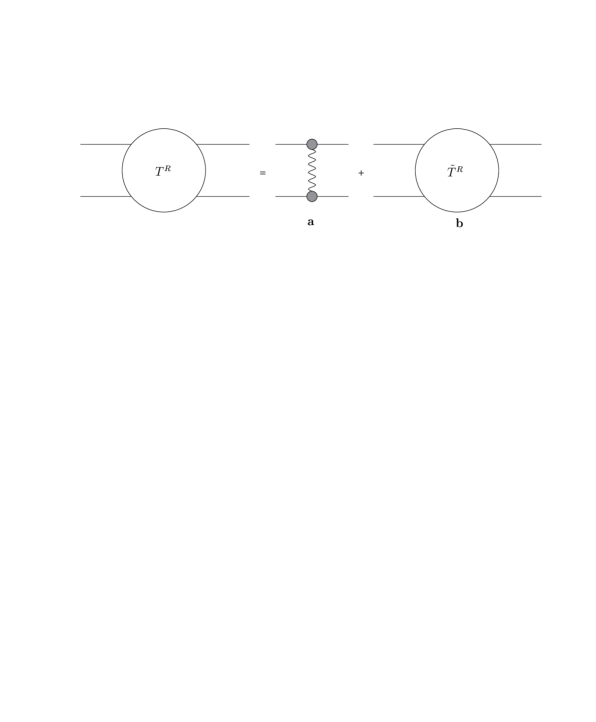
FIG. 3.:

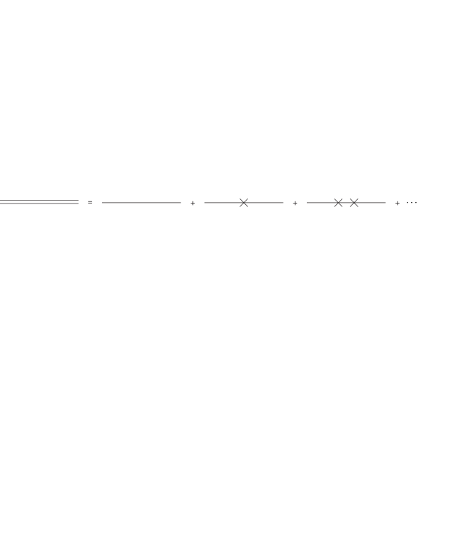
FIG. 4.:

FIG. 5.:

FIG. 6.:

REFERENCES

- [1] B. Adeva et al., CERN proposal CERN/SPSLC 95-1 (1995).
- [2] H.-Ch. Schröder et al., Phys. Lett. B 469 (1999) 25; D. Gotta, Newslett. 15, 276 (1999).
- [3] ”DANE exotic atom research: the DEAR proposal”, By DEAR collaboration (R. Baldini et al.), Preprint LNF-95-055-IR, (1995).
- [4] M. Iwasaki et al, Phys. Rev. Lett. 78 (1997) 3067; Nucl. Phys. A 639 (1998) 501.
- [5] S. Deser, M.L. Goldberger, K. Baumann, and W. Thirring, Phys. Rev. 96, 774 (1954).
- [6] T.L. Trueman, Nucl. Phys. 26, 57 (1961).
- [7] G. Rasche and W. S. Woolcock, Nucl. Phys. A 381, 405 (1982); U. Moor, G. Rasche, and W.S. Woolcock, Nucl. Phys. A 587, 747 (1995); A. Gashi, G.C. Oades, G. Rasche, and W.S. Woolcock, Nucl. Phys. A 628, 101 (1998);
- [8] A. Gashi, G.C. Oades, G. Rasche, and W.S. Woolcock, Preprint hep-ph/0108116.
- [9] G. Rasche, talk at the HADATOM01 workshop, 11-12 October 2001, Bern, Switzerland.
- [10] D. Sigg, A. Badertscher, P.F.A. Goudsmit, H.J. Leisi, and G.C. Oades, Nucl. Phys. A 609, 310 (1996).
- [11] B. Tromborg, S. Waldenstrom, and I. Overbo, Phys. Rev. D 15, 725 (1977); Helv. Phys. Acta 51, 584 (1978).
- [12] R. Koch and E. Pietarinen, Nucl. Phys. A 336, 331 (1980).
- [13] E. Sauter, Nuovo Cim. 61 A, 515 (1969); 6 A, 335 (1971).
- [14] G.C. Oades and G. Rasche, Helv. Phys. Acta 44, 5 (1971); 44, 160 (1971); A. Gashi, E. Matsinos, G.C. Oades, G. Rasche, and W.S. Woolcock, Nucl. Phys. A 686, 447 (2001); 686, 463 (2001).
- [15] H. Zimmermann, Helv. Phys. Acta 47, 130 (1974); 48, 191 (1975).
- [16] A. Gashi, E. Matsinos, G.C. Oades, G. Rasche, and W.S. Woolcock, Preprint hep-ph/0009081.
- [17] H. Jallouli and H. Sazdjian, Phys. Rev. D 58, 014011 (1998); H. Sazdjian, Preprint hep-ph/9809425; Phys.Lett. B 490, 203 (2000); V.E. Lyubovitskij and A.G. Rusetsky, Phys. Lett. B 389, 181 (1996); V.E. Lyubovitskij, E.Z. Lipartia, and A.G. Rusetsky, JETP Lett. 66, 783 (1997); M.A. Ivanov, V.E. Lyubovitskij, E.Z. Lipartia, and A.G. Rusetsky, Phys. Rev. D 58, 094024 (1998).
- [18] P. Labelle and K. Buckley, Preprint hep-ph/9804201; X. Kong and F. Ravndal, Phys. Rev. D 59, 014031 (1999); Phys. Rev. D 61, 077506 (2000); B.R. Holstein, Phys. Rev. D 60, 114030 (1999); D. Eiras and J. Soto, Newslett. 15, 181 (1999); Phys. Rev. D 61, 114027 (2000); Phys. Lett. B 491, 101 (2000).
- [19] A. Gall, J. Gasser, V.E. Lyubovitskij, and A. Rusetsky, Phys. Lett. B 462, 335 (1999).
- [20] J. Gasser, V.E. Lyubovitskij, and A. Rusetsky, Phys. Lett. B 471, 244 (1999).
- [21] V.E. Lyubovitskij and A. Rusetsky, Phys. Lett. B 494, 9 (2000).
- [22] A. Gall, J. Gasser, V.E. Lyubovitskij, and A. Rusetsky, Phys. Rev. D 64, 016008 (2001).
- [23] V.E. Lyubovitskij, T. Gutsche, A. Faessler, and R. Vinh Mau, Preprint hep-ph/0109213.
- [24] J. Gasser, V.E. Lyubovitskij, and A. Rusetsky, Newslett. 15, 197 (1999).
- [25] N. Fettes and U. Meissner, Nucl. Phys. A 693, 693 (2001).
- [26] G.P. Lepage, Preprint nucl-th/9706029.
- [27] M.C. Birse, J.A. McGovern, and K.G. Richardson, Preprint hep-ph/9708435; Phys. Lett. B 464, 169 (1999).
- [28] D.B. Kaplan, M.J. Savage, and M.B. Wise, Nucl. Phys. B 534, 329 (1998); U. van Kolck, Nucl. Phys. A 645, 273 (1999); Prog. Part. Nucl. Phys. 43, 337 (1999).
- [29] V. Antonelli, A. Gall, J. Gasser, and A. Rusetsky, Ann. Phys. 286, 108 (2000).
- [30] A. Nandy, Phys. Rev. D 5, 1531 (1972).
- [31] J. Schwinger, J. Math. Phys. 5, 1606 (1964).
- [32] H. Feshbach, Ann. Phys. 5, 357 (1958); 19, 287 (1962).