QCD string model for hybrid adiabatic potentials

Abstract

Hybrid adiabatic potentials are considered in the framework of the QCD string model. The einbein field formalism is applied to obtain the large-distance behaviour of adiabatic potentials. The calculated excitation curves are shown to be the result of interplay between potential-type longitudinal and string-type transverse vibrations. The results are compared with recent lattice data.

1 Introduction

There is no doubts now that hadrons with explicit gluonic degrees of freedom should exist. This idea is supported not only by general arguments from QCD, but also by lattice simulations of pure Yang-Mills theory. In the absence of exact analytical methods of nonperturbative QCD one relies upon models to describe gluonic mesons, so that the challenging question arises of how to introduce effective degrees of freedom for soft (constituent) glue.

There is a lot of indications now that gluonic mesons are already found experimentally, but the conclusive evidences have never been presented; there is no hope that in the nearest future data analyses could shed light on this problem and to offer necessary feedback for model building. The current situation is such that the predictions of different models on hadronic spectra and decays are involved in order to pin-point the signatures for gluonic mesons.

On the other hand, lattice calculations are now accurate enough to provide reliable data on constituent glue and to check model predictions. In this regard recent measurements of gluelump [1] and hybrid adiabatic potentials [2] are of particular interest. These simulations measure the spectrum of the glue in the presence of infinitely heavy adjoint source (gluelump) and in the presence of static quark and antiquark separated by some distance $R$. These systems are the simplest ones and play the role of hydrogen atom of soft glue studies, as the complicated problem of the centre-of-mass motion separation is not relevant here.

Hybrid adiabatic potentials enter heavy hybrid mass estimations in the Born-Oppenheimer approximation: these potentials are to be inserted into $Q\bar{Q}$ Schroedinger equation in order to obtain spectra of hybrids with heavy quarks. The large $R$ limit is interesting per se, as the formation of confining string is expected at large distances, so the direct measurements of the string fluctuations become available and the possibility exists to discriminate between different models of the effective string degrees of freedom.

2 Constituent gluons at the end of the string

The notion of confinement is usually described in terms of area law asymptotics for the Wilson loop expectation value, defined as an integral along some closed contour $C$, averaged over gluonic vacuum configurations:

$$\langle W(C)\rangle=\mathrm{Tr}\langle P\exp{\;ig\oint_{C}A_{\mu}dz_{\mu}}\rangle,$$ (1)

where trace is taken over colour indices. The area law asymptotics implies that

$$\langle W(C)\rangle\rightarrow N_{C}\exp(-\sigma S),$$ (2)

where $N_{C}$ is the number of colours, $\sigma$ is the string tension, and $S$ is the surface bound by the closed contour $C$. As the initial expression (1) depends only on the contour, the area in (2) should depend only on the contour too, and should be the minimal area.

The area law asymptotics provides the action of the string, and in the case of minimal area this string is also ”minimal”. The effective string model should be arranged to allow the extra degrees of freedom to populate the string and to be responsible for more complicated string configurations. In what follows these extra degrees of freedom are defined in the framework of the QCD string model. This model deals with quarks and point-like gluons propagating in the confining QCD vacuum, and is based on Vacuum Background Correlators method [3].

The QCD string model for gluons is derived from the perturbation theory in the nonperturbative confining background developed in [4]. The main idea is to split the gauge field as

$$A_{\mu}=B_{\mu}+a_{\mu},$$ (3)

which allows to distinguish clearly between confining gluonic field configurations $B_{\mu}$ and confined valence gluons $a_{\mu}$. Confining QCD vacuum is given by the set of gauge invariant field strength correlators made of $B_{\mu}$, which are responsible for the area law asymptotics (2), while the valence gluons are treated as perturbation at this confining background.

The starting point is the Green function for the gluon propagating in the given external field $B_{\mu}$ [4]:

$$G_{\mu\nu}(x,y)=(D^{2}(B)\delta_{\mu\nu}+2igF_{\mu\nu}(B))^{-1}.$$ (4)

The term, proportional to $F_{\mu\nu}(B)$ is responsible for the gluon spin interaction, it can be treated as perturbation [5], and we neglect it for a moment. The next step is to use Feynman-Schwinger representation for the quark-antiquark-gluon Green function, which, for the case of static quark and antiquark, is reduced to the form

$$G(x_{g},y_{g})=\int ds\int Dz_{g}\exp(-K_{g})\langle{\cal W}\rangle_{B},$$ (5)

where angular brackets mean averaging over background field. The quantity $K_{g}$ is the kinetic energy of gluon (to be specified below), and all the dependence on the vacuum background field is contained in the generalized Wilson loop $\cal W$, depicted in Fig.1.

Figure 1: Hybrid Wilson loop.

The main assumption of the QCD string model is the minimal area law, which yields for the configuration $\cal W$ the form [6]

$$\langle{\cal W}\rangle_{B}=\frac{N_{C}^{2}-1}{2}\exp(-\sigma(S_{1}+S_{2})),$$ (6)

where $S_{1}$ and $S_{2}$ are the minimal areas inside the contours formed by quark and gluon and antiquark and gluon trajectories correspondingly.

3 Einbein field form of the gluonic Lagrangian

To define the form of gluon kinetic energy we note that the action of a particle in the external vector field is invariant under reparametrization transformations, and, of course, it remains true after averaging over the background. So, to proceed further we are to fix the gauge, and the most natural way to do this is to identify the proper time $\tau$ of the path integral representation with the physical time $x_{g}^{0}$. Then the action of the system can be immediately read out of the representation (5):

$$A=\int d\tau\left\{-\frac{\mu}{2}+\frac{\mu\dot{r}^{2}}{2}-\sigma\int^{1}_{0}d\beta_{1}\sqrt{(\dot{w}_{1}w_{1}^{\prime})^{2}-\dot{w}_{1}^{2}w^{{}^{\prime}2}_{1}}-\right.$$

$$\left.-\sigma\int^{1}_{0}d\beta_{2}\sqrt{(\dot{w}_{2}w_{2}^{\prime})^{2}-\dot{w}_{2}^{2}w^{{}^{\prime}2}_{2}}\right\},$$ (7)

where the minimal surfaces $S_{1}$ and $S_{2}$ are parametrized by the coordinates $w_{i\mu}(\tau,\beta_{i}),~{}i=1,2,~{}\dot{w}_{i\mu}=\frac{\partial w_{i\mu}}{\partial\tau},~{}w^{\prime}_{i\mu}=\frac{\partial w_{i\mu}}{\partial\beta_{i}}.$ In what follows the straight-line ansatz is chosen for the minimal surface:

$$w_{i0}=\tau,~{}~{}~{}\vec{w}_{1,2}=\pm(1-\beta)\frac{\vec{R}}{2}+\beta\vec{r}.$$ (8)

The quantity $\mu=\mu(\tau)$ in the expression (7) is the so-called einbein field [7]; here one is forced to introduce it, as it is the only way to obtain the meaningful dynamics for the massless particle.

Let us introduce another set of einbein fields, $\nu_{i}=\nu_{i}(\tau,\beta_{i})$ to get rid of Nambu-Goto square roots in (7) [8]. The resulting Lagrangian takes the form

$$L=-\frac{\mu}{2}+\frac{\mu\dot{r}^{2}}{2}-\int^{1}_{0}d\beta_{1}\frac{\sigma^{2}r^{2}_{1}}{2\nu_{1}}-\int^{1}_{0}d\beta_{1}\frac{\nu_{1}}{2}(1-\beta_{1}^{2}l_{1}^{2})-$$

$$-\int^{1}_{0}d\beta_{2}\frac{\sigma^{2}r^{2}_{2}}{2\nu_{2}}-\int^{1}_{0}d\beta_{2}\frac{\nu_{2}}{2}(1-\beta_{2}^{2}l_{2}^{2}),$$

$$l^{2}_{1,2}=\dot{r}^{2}-\frac{1}{r^{2}_{1,2}}(\vec{r}_{1,2}\dot{\vec{r}})^{2},~{}~{}\vec{r}_{1,2}=\vec{r}\pm\frac{\vec{R}}{2},$$ (9)

and the corresponding Hamiltonian reads

$$H=H_{0}+\frac{\mu}{2}+\int^{1}_{0}d\beta_{1}\frac{\sigma^{2}r^{2}_{1}}{2\nu_{1}}+\int^{1}_{0}d\beta_{2}\frac{\sigma^{2}r^{2}_{2}}{\nu_{2}}+\int^{1}_{0}d\beta_{1}\frac{\nu}{2}+\int^{1}_{0}d\beta_{2}\frac{\nu_{2}}{2},$$ (10)

$$H_{0}=\frac{p^{2}}{2(\mu+J_{1}+J_{2})}+$$

$$\frac{1}{2\Delta(\mu+J_{1}+J_{2})}\left\{\frac{(\vec{p}\vec{r}_{1})^{2}}{r^{2}_{1}}J_{1}(\mu+J_{1})+\frac{(\vec{p}\vec{r}_{2})^{2}}{r^{2}_{2}}J_{2}(\mu+J_{2})+\right.$$

$$\left.\frac{2J_{1}J_{2}}{r^{2}_{1}r^{2}_{2}}(\vec{r}_{1}\vec{r}_{2})(\vec{p}\vec{r}_{1})(\vec{p}\vec{r}_{2})\right\},$$ (11)

$$\Delta=(\mu+J_{1})(\mu+J_{2})-J_{1}J_{2}\frac{(\vec{r}_{1}\vec{r}_{2})^{2}}{r^{2}_{1}r^{2}_{2}},~{}~{}J_{i}=\int^{1}_{0}d\beta_{i}\beta_{i}^{2}\nu_{i}(\beta_{i}),~{}~{}i=1,2.$$

At first glance, the Hamiltonian (11) looks tractable. Clearly, quantities $\mu$ and $\nu_{i}$ play the role of gluon constituent mass and energy density distributions along the string respectively. Nevertheless, introducing einbeins does not do miracles for us. These redundant variables are to be found from the conditions

$$\frac{\partial H}{\partial\mu}=0,~{}~{}\frac{\delta H}{\delta\nu_{i}(\beta_{i})}=0,$$ (12)

as the equations (12) play the role of second class constraints. One should do it before quantization and substitute the resulting values into the Hamiltonian. Such procedure is hardly possible analytically even at the classical level, and after quantization these extremal values of einbeins would become nonlinear operator functions of coordinates and momenta with inevitable ordering problems arising.

In what follows we use the approximate einbein field method, which treats the einbeins as $c$-number variational parameters. The eigenvalues of the Hamiltonian (11) are found as functions of $\mu$ and $\nu_{i}$ and minimized with respect to eibeins to obtain the physical spectrum. Such procedure works surprisingly well in the QCD string model calculations, with the accuracy of about 5-10% [9].

4 Dynamical regimes of the gluonic Hamiltonian

Even with the simplifying assumptions of the approximate einbein field method the problem remains complicated due to the presence of the terms $J_{i}$ responsible for the string inertia. If one neglect these terms, then the einbeins are eliminated explicitly from the Hamiltonian (11), and one arrives at the potential model Hamiltonian

$$H=\sqrt{p^{2}}+\sigma r_{1}+\sigma r_{2}.$$ (13)

It appears, however, that the neglect of string inertia is justified only for $R\leq 1/\sqrt{\sigma}$ [10]. Indeed, in the einbein field method the potential regime corresponds to the case of $\nu_{i}$ independent of $\beta_{i}$. For example, for $R\ll 1/\sqrt{\sigma}$ one has

$$E_{n}(R)=2^{3/2}\sigma^{1/2}(n+3/2)^{1/2}+\frac{\sigma^{3/2}R^{2}}{2^{3/2}(n+3/2)^{1/2}},$$ (14)

$$\mu_{n}(R)=2^{1/2}\sigma^{1/2}(n+3/2)^{1/2}-\frac{\sigma^{3/2}R^{2}}{2^{5/2}(n+3/2)^{1/2}},$$

$$\nu_{1,2n}(R)=\frac{(n+3/2)^{1/2}\sigma^{1/2}}{2^{1/2}}+\frac{3\sigma^{3/2}R^{2}}{2^{7/2}(n+3/2)^{1/2}},$$

where $n$ is the number of oscillator quanta. The last line in (14) readily gives $J_{1,2}/\mu\approx 1/6$. The situation here is similar to the one in the light quark, glueball and gluelump sectors: the corrections due to the string inertia are sizeable, but not large, and can be taken into account as perturbation [5].

The situation changes drastically for the case of large $R,~{}R\gg 1/\sqrt{\sigma}$. Here one has

$$E_{n}(R)=\sigma R+\frac{3}{2^{1/3}}\sigma^{1/3}\frac{(n+3/2)^{2/3}}{R^{1/3}},$$ (15)

$$\mu_{n}(R)=\frac{4\sigma^{1/3}(n+3/2)^{2/3}}{R^{1/3}},~{}~{}\nu_{1,2n}(R)=\frac{\sigma R}{2}.$$

In this case $J_{1,2}=\frac{1}{6}\sigma R\gg\mu_{n}$, and the potential regime becomes unadequate.

The case of large $R$ can be treated exactly in the einbein field method. There are two different kinds of excitations, along the $Q\bar{Q}$ axis and in the transverse direction, which are decoupled in the limit of large $R$. In this case one has

$$E_{n}(R)=\sigma R+\frac{3}{2^{1/3}}\frac{\sigma^{1/3}(n_{z}+1/2)^{2/3}}{R^{1/3}}+\frac{2\cdot 3^{1/2}}{R}(n_{\rho}+\Lambda+1),$$ (16)

where $\Lambda=\left|\frac{\vec{L}\vec{R}}{R}\right|$ is the projection of orbital momentum onto $Q\bar{Q}$ axis ($z$ axis). Note, that the subleading corrections due to the longitudinal and transverse vibrations are different, the former behaves as $\frac{\sigma}{R}^{1/3}$, like the pure potential regime (15), while the latter displays string-type behaviour $\sim\Lambda/R$.

The quasiclassical limit of large $\Lambda$, where only rotations around $z$ axis are taken into account, was found for the Hamiltonian (11) in [10]. The large $R$ limit reads

$$E(R)=\sigma R+2\sqrt{3}\frac{\Lambda}{R},$$ (17)

which should be compared with the predictions from naive Nambu-Goto string model

$$E(R)=\sigma R+\frac{\pi\Lambda}{R}$$ (18)

in the small oscillation limit. The coefficients $\pi$ and $2\sqrt{3}$ are close to each other, and differ mainly due to the fact that string configurations differ: there are two straight-line strings in the QCD string model, and one continuous string in the Nambu-Goto case. The quasiclassical excitation curve [10] is shown in Fig.2 together with the Nambu-Goto (18) and potential curves. Note the absence of the unphysical divergent $1/R$ behaviour at small $R$ both for quasiclassical and potential curves.

Figure 2: Adiabatic hybrid potentials in various regimes. Quasiclassical (solid line), potential (dashed), and flux-tube (dotted) curves for $n_{z}=n_{\rho}=0$ and $\Lambda=1,2,3$. The lowest curve is $\sigma R$. $\sigma=0.22$GeV².

Figure 3: Corrections to linear behaviour of potentials. QCD string (solid line), potential (dashed), and flux-tube (dotted) curves; $n_{z}=n_{\rho}=0$; $\sigma=0.22$GeV².

The dominant subleading regime is defined by longitudinal motion: even if no longitudinal quanta are excited, there is the contribution of zero longitudinal oscillations in (16). Still, if the distances are not asymptotically large, the potential regime is substantionally contaminated by the string-type transverse vibrations.

Corresponding corrections to linear behaviour for QCD string (16), potential regime (15), and Nambu-Goto string (18) are shown in Fig.3.

There is no QCD string calculations for large distances with proper account of gluon spin yet, so the direct comparison with lattice results is premature. Nevertheless, some preliminary conclusions can be drawn. The behaviour (16) displays the most pronounced difference between QCD string and other models for constituent glue. In the flux tube model [11] the string vibrations are caused by string phonons, so one expects the Nambu-Goto behaviour (18) at large distances. In contrast to this, here the string vibrations are caused by pointlike valence gluons. In the constituent gluon model with linear potential [12] one should have the potential-type behaviour (15), while in the QCD string model the confining force follows from the minimal area law, and, as a consequence, the contributions from the string inertia leave room for the string-type vibrations.

5 Full QCD string calculations in the potential regime

Let us now consider the regime of ”small” $R$ relevant to the heavy hybrid mass estimations. Actually these distances are not very small: one expects that in the case of very heavy quarks the hybrid resides in the bottom of the potential well given by the adiabatic curve. The lattice results [2] are not very accurate for small $R$, but the message is quite clear: the bottom of the potential well is somewhere around 0.25 fm for lowest curves.

If only confining force is taken into account, the QCD string model predicts the oscillator potential (14) with the minimum at $R=0$. However, the minimum is shifted, if the long range confining force is augmented by the short range Coulomb interaction, which is taken in the form

$$V_{c}=-\frac{3}{2}\frac{\alpha_{s}}{r_{1}}-\frac{3}{2}\frac{\alpha_{s}}{r_{2}}+\frac{\alpha_{s}}{6R}.$$ (19)

The coefficients in (19) are in accordance with the colour content of the $Q\bar{Q}g$ system. Note that the $Q\bar{Q}$ Coulomb force is repulsive. It is in contrast to the flux tube model [11], where the string phonons do not carry colour quantum number, so that the $Q\bar{Q}$ pair is in the colour singlet state, and Coulomb interaction is attractive. In the so-called single-bead version of the flux tube model the minimum due the confining force is at $R=0$, and attractive Coulomb force cannot shift it, so the single-bead version seems to be ruled out by lattice data. As the gluon energies of [2] lie well below the curves (18), the simple Nambu-Goto regime is excluded too.

Below we present the results of the QCD string model with Coulomb force included, for small and intermediate values of $R$. The calculations were performed in the potential regime, and the string inertia was taken into account perturbatively, which is justified by arguments given above.

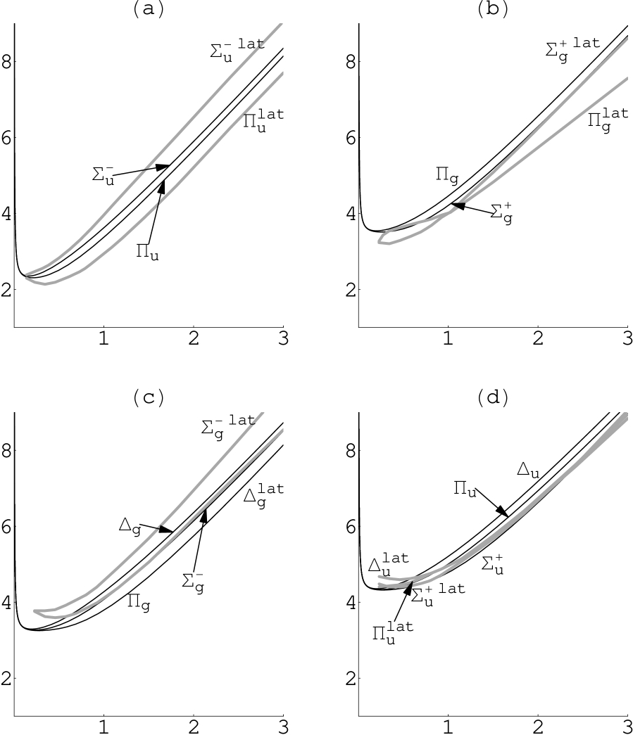
Figure 4: Hybrid potentials in full QCD string model (thin solid curves) compared to lattice results (thick light curves). $Q\bar{Q}$ distance $R$ is in units $2r_{0}\approx$ 1 fm and potentials $V$ are in units $1/r_{0}$.

Varying over $\mu_{i}$ with result $\mu_{1,2}=\sigma r_{1,2}$, we obtain the Hamiltonian in the form

$$\tilde{H}=\frac{\mu}{2}+\frac{p^{2}}{2\mu}+\sigma(r_{1}+r_{2})-\frac{3\alpha_{s}}{2}\left(\frac{1}{r_{1}}+\frac{1}{r_{2}}\right)+\frac{\alpha_{s}}{6R}.$$ (20)

We calculate unperturbed adiabatic energy levels variationally with Gaussian wave functions used,

$$E_{jl\Lambda}(\mu,R)=\langle\Psi_{jl\Lambda}(\vec{r})|\tilde{H}(\mu,\vec{r},\vec{R})|\Psi_{jl\Lambda}(\vec{r})\rangle\equiv\langle\tilde{H}\rangle_{jl\Lambda},$$ (21)

$$\Psi_{jl\Lambda}(\vec{r})=\phi_{l}(\vec{r})\sum_{\mu_{1}\mu_{2}}C^{j\Lambda}_{l\mu_{1}l\mu_{2}}Y_{l\mu_{1}}\left(\frac{\vec{r}}{r}\right)s_{1\mu_{2}},$$ (22)

where $s$ is the spin wave function. The unpertubed adiabatic potentials

$$V^{0}_{jl\Lambda}(R)=E_{jl\Lambda}(\mu^{*}(R),R),$$ (23)

depend on the extremal value $\mu^{*}$ defined from the condition $\frac{\partial E_{jl\Lambda}(\mu,R)}{\partial\mu}=0$.

The string correction Hamiltonian at $\nu\ll\mu$ after integrating out $\nu$ reads

$$H^{\mathrm{string}}=-\frac{\sigma}{6\mu^{2}}\left(\frac{1}{r_{1}}L_{1}^{2}+\frac{1}{r_{2}}L_{2}^{2}\right)=$$

$$-\frac{\sigma}{6\mu^{2}}\left\{\left(\frac{1}{r_{1}}+\frac{1}{r_{2}}\right)\left[L^{2}+\frac{1}{4}\left(R_{j}p_{k}R_{j}p_{k}-R_{j}p_{k}R_{k}p_{j}\right)\right]+\right.$$

$$\left.\frac{1}{2}\left(\frac{1}{r_{1}}-\frac{1}{r_{2}}\right)\left[r_{j}p_{k}R_{j}p_{k}-r_{j}p_{k}R_{k}p_{j}+R_{j}p_{k}r_{j}p_{k}-R_{j}p_{k}r_{k}p_{j}\right]\right\},$$ (24)

where $\vec{L}_{1,2}=\vec{r}_{1,2}\times\vec{p},~{}\vec{L}=\vec{r}\times\vec{p}$.

Here we estimate the contribution of the string correction (24) taking it at $R=0$, where it reads

$$V_{l}^{\mathrm{string}}=-\frac{\sigma l(l+1)}{3\mu_{l}^{*2}}\langle\frac{1}{r}\rangle_{l}.$$ (25)

By the same way we consider spin-orbit correction at $R=0$,

$$V^{\mathrm{SO}}_{jl}=-\frac{\sigma\vec{S}\vec{L}}{2\mu_{l}^{*2}}\langle\frac{1}{r}\rangle_{l},$$ (26)

where $\vec{S}\vec{L}=\frac{1}{2}(j(j+1)-l(l+1)-2)$. We also subtract a constant that corresponds to gluon self-energy. From comparison with lattice data [2] its value is found to be $\Sigma_{\mathrm{gl}}=473$ MeV.

In Fig.4 (a)-(d) potential

$$V_{jl\Lambda}(R)=V^{0}_{jl\Lambda}(R)+V_{l}^{\mathrm{string}}+V^{\mathrm{SO}}_{jl}-\Sigma_{\mathrm{gl}}$$ (27)

(solid curves) is compared to lattice potentials from [2] (thick grey curves). Parameters $\alpha_{s}=0.225,~{}\sigma=0.227$ GeV² are taken from fit of the lattice Coulomb+linear ground-state potential. In the Fig. 4 standard notations from the physics of atomic molecules are used.

In Table 1 the quantum numbers of levels, shown in Fig.4 (a)-(d), are listed, in terms of $j,l,\Lambda$, and atomic notations. Note, that in the QCD string model the gluon is effectively massive and has three polarizations [5], and only two of them are excited with magnetic components of field strength correlators, used in the lattice calculations. It is just these states which are listed in the Table 1. For more details justifying such correspondance see [5].

Table 1: Quantum numbers of levels of Fig. 4

(a)	$j=1,~{}l=1,~{}\Lambda=0,1$	$\Sigma_{u}^{-},~{}\Pi_{u}$
(b)	$j=1,~{}l=2,~{}\Lambda=0,1$	$\Sigma_{g}^{+},~{}\Pi_{g}$
(c)	$j=2,~{}l=2,~{}\Lambda=0,1,2$	$\Sigma_{g}^{-},~{}\Pi_{g},~{}\Delta_{g}$
(d)	$j=2,~{}l=3,~{}\Lambda=0,1,2$	$\Sigma_{u}^{+},~{}\Pi_{u},~{}\Delta_{u}$

6 Conclusions

The first results of the QCD string model for the hybrid adiabatic potentials look rather encouraging. We have obtained the reasonable agreement with lattice data at small and intermediate interquark distances. The most interesting feature of the QCD string model is the large distance behaviour of the adiabatic potentials, with potential-type longitudinal and string-type transverse vibrations. The full calculations of large distance behaviour with proper account of gluonic spin are in progress now.

7 Acknowledgements

Financial support of RFFI grants 00-02-17836, 00-15-96786, INTAS-RFFI grant IR-97-232 and INTAS CALL 2000-110 is gratefully acknowledged.

References

- [1] Foster, M. and Michael, C., Phys.Rev., D59, 094509 (1999)
- [2] Juge, K.J., Kuti, J., and Morningstar, C., Proc. LATTICE 98, Nucl. Phys. Proc. Suppl. 73, 590 (1999)
- [3] Simonov, Yu.A., Lectures at the XVII Int. School of Physics, Lisbon (1999)
- [4] Simonov, Yu.A., Phys.At.Nucl., 58, 107 (1995)
-
[5]
Simonov, Yu.A., Nucl.Phys., B592, 350 (2000)
Kaidalov, A.B. and Simonov, Yu.A., Phys.Lett. B477, 163 (2000) - [6] Kalashnikova, Yu.S. and Yufryakov, Yu.B., Phys.Lett. B359, 175 (1995); Phys.Atom.Nucl., 60, 307 (1995)
- [7] Kalashnikova, Yu.S. and Nefediev, A.V., Phys.At.Nucl., 60, 1389 (1997)
- [8] Dubin, A.Yu., Kaidalov, A.B. and Simonov, Yu.A., Phys.Lett., B323, 41 (1994); Phys.At.Nucl, 56, 1745 (1993)
- [9] Morgunov V.L., Nefediev, A.V. and Simonov, Yu.A., Phys.Lett., B459, 653 (1999)
- [10] Kalashnikova, Yu.S. and Kuzmenko, D.S., hep-ph/0006073
- [11] Isgur, N. and Paton, J., Phys.Rev., D31, 2910 91985)
- [12] Horn, D. and Mandula, J., Phys.Rev., D17, 537 (1978)