Theoretical progress in describing the $B$-meson lifetimes

Abstract:

The present status of the theoretical estimates of the difference between the widths of the neutral $B_{s}$-mesons and of the $B$-meson lifetime ratios is reviewed. In particular, the lattice results for the matrix elements of the relevant $\Delta B=2$ operators are updated and the first lattice QCD results for the matrix elements of $\Delta B=0$ operators are presented. In both cases, the NLO perturbative QCD corrections in the coefficient functions have been included. The theoretically updated results are: $(\Delta\Gamma/\Gamma)_{B_{s}}=7\pm 4\ \%$, ${\tau(B^{+})/\tau(B_{d})}=1.07(3)$ and ${\tau(B_{s})/\tau(B_{d})}=1.00(2)$.

To make it clear and simple, I split the discussion into two parts:

• $(\Delta\Gamma/\Gamma)_{B_{s}}$, the quantity that recently attracted quite a bit of attention among theorists and for which the experimental upper limit has been set at [1]:

  $$\left({\Delta\Gamma\over\Gamma}\right)_{B_{s}}<0.31\quad(95\%\ {\rm C.L.})\,.$$ (1)

• $\tau(B_{u(s)})/\tau(B_{d})$ have been measured quite accurately [1]

  $${\tau(B_{u})\over\tau(B_{d})}=1.07(2)\,,\quad{\tau(B_{s})\over\tau(B_{d})}=0.95(4)\;.$$ (2)

  Important theoretical progress in computing these ratios has been made this year. I will not discuss the theoretical predictions for the ratio ${\tau(\Lambda_{b})/\tau(B_{d})}$, where, in my opinion, substantial progress is yet to be made.

Theoretical set-up for both of the above topics relies on the hypothesis of the (global and local) quark–hadron duality [2]. The validity of that assumption is not totally clear, although the impressive agreement of many theoretical predictions in $\tau$-physics (for which the duality has been assumed) with the precise experimental data is very encouraging [3].

1 WIDTH DIFFERENCE OF THE $B_{S}^{0}$-SYSTEM

The Orsay group broke the duality problem a little bit open by demonstrating that in the combined $N_{c}\to\infty$ and SV limit , the quark–hadron duality for $\Delta\Gamma_{B_{s}}$ indeed works [4]. They actually showed that the two channels, $B_{s}^{0}\to D_{s}\overline{D}_{s}$, $D_{s}^{\ast}\overline{D}_{s}^{\ast}$ (S-wave), saturate the partonic expression for $\Delta\Gamma_{B_{s}}$. Out of that limit, however, the quark–hadron duality is again an assumption.

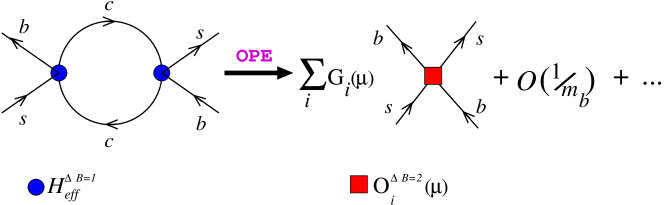
Figure 1: Heavy quark expansion: the non-local T-product of the l.h.s. (with the doubly inserted ${\cal H}_{eff}^{\Delta B=1}$) is expanded in the series in $1/m_{b}$, each coefficient being the sum of local ${\Delta B=2}$ operators.

The (modern) theoretical expression for $\Delta\Gamma_{B_{s}}$ has been derived in ref. [8], where the operator product expansion (OPE) has been applied to compute the absorptive amplitude for the $B_{s}\to\bar{B}_{s}$ transition.  The high energy scale is provided by the inverse $b$-quark mass, which is why this expansion is usually referred to as the heavy quark expansion (sketched in fig. 1). The final expression of ref. [8] looks as follows:

$$\Delta\Gamma_{B_{s}}={G_{F}^{2}m_{b}^{2}\over 12\pi m_{B_{s}}}|V_{cb}^{\ast}V_{cs}|^{2}\ \biggl{\{}G_{1}(\mu)\langle\bar{B}_{s}|O_{1}(\mu)|B_{s}\rangle+G_{2}(\mu)\langle\bar{B}_{s}|O_{2}(\mu)|B_{s}\rangle+\delta_{1/m_{b}}\biggr{\}}\ ,$$ (3)

where the flavour structure of the operators $O_{1,2}(\mu)$ is $\Delta B=2$; $\delta_{1/m_{b}}$ contains all the contributions from the $1/m_{b}$ corrections to the first two terms. Corrections $\propto 1/m_{b}^{n}$ ($n\geq 2$) are neglected.

• Short distance physics is encoded in the functions $G_{1,2}(\mu)$ which are the combinations of $\Delta B=1$ Wilson coefficients. The next-to-leading order (NLO) corrections to these functions have been computed in ref. [9], where the authors also kept the ratio $m_{c}/m_{b}$ different from zero. Of conceptual importance is the fact that they explicitly verified the infrared safety of the functions $G_{1,2}^{\rm NLO}(\mu)$, as anticipated years before, in ref. [10]. Phenomenologically, however, the (subleading) corrections are uncomfortably large. For example, the dominant term changes as

  $${G_{2}^{\rm NLO}(m_{b})-G_{2}^{\rm LO}(m_{b})\over G_{2}^{\rm LO}(m_{b})}\simeq-0.35\;,$$ (4)

  i.e. the radiative corrections lower $G_{2}(m_{b})$ by $35\%$. The residual scale dependence of $\Delta B=1$ Wilson coefficients entering the functions $G_{1,2}(m_{b})$ is customarily estimated by varying the renormalization scale from $\mu=m_{b}/2$ to $\mu=2m_{b}$, which amounts to an error of $-20\%$ and $+15\%$, respectively;

• Long distance QCD dynamics is described by the matrix elements, which are parametrized as

  $$\langle\bar{B}_{s}|O_{1}(\mu)|B_{s}\rangle\equiv\langle\bar{B}_{s}|(\bar{b}s)_{V-A}(\bar{b}s)_{V-A}|B_{s}\rangle={8\over 3}f_{B_{s}}^{2}m_{B_{s}}^{2}B_{1}(\mu)\,,$$ (5)

  (6)

  $$\langle\bar{B}_{s}|O_{2}(\mu)|B_{s}\rangle\equiv\langle\bar{B}_{s}|(\bar{b}s)_{S-P}(\bar{b}s)_{S-P}|B_{s}\rangle=-{5\over 3}\left({f_{B_{s}}m_{B_{s}}^{2}\over m_{b}(\mu)+m_{s}(\mu)}\right)^{2}B_{2}(\mu)\,,$$ (7)

  (8)

  $$\langle\bar{B}_{s}|O_{3}(\mu)|B_{s}\rangle\equiv\langle\bar{B}_{s}|(\bar{b}^{i}s^{j})_{S-P}(\bar{b}^{j}s^{i})_{S-P}|B_{s}\rangle={1\over 3}\left({f_{B_{s}}m_{B_{s}}^{2}\over m_{b}(\mu)+m_{s}(\mu)}\right)^{2}B_{3}(\mu)\,,$$ (9)

  where the third operator has the same Dirac structure as $O_{2}$ but with reversed colour indices ($i,j$), and hence mixes with $O_{2}$ under renormalization. The above $B$-parameters are all equal to unity in the vacuum saturation approximation (VSA). A priori, VSA gives a gross estimate and one has to include the (non-factorizable) non-perturbative QCD effects. QCD simulations on the lattice represent a suitable method for that part of the job, which I discuss in the next subsection.

1.1 $B$-parameters (novelties from the lattice)

I would like to stress that, in principle, lattice QCD approach allows the fully non-perturbative estimate of the hadronic quantities to an arbitrary accuracy. In practice, however, many approximations need to be made which, besides the statistical, introduce various systematic uncertainties in the final results. The steady progress in increasing the computational power, combined with various theoretical improvements, helps reducing ever more of those systematic uncertainties. This is why the lattice QCD approach is so attractive.

The ultimate goal in the study of the heavy quark physics on the lattice is to produce the results by simulating the $b$-quark directly, in the full QCD. Since we are still quite far from that point, as I will briefly explain in what follows, we use various ways to treat the heavy quark on the lattice and thus various ways to compute the $B$-parameters of eq. (5):

• HQET: After discretizing the HQET lagrangian (to make it tractable for a lattice study), the matrix elements from eq. (5) were computed in ref. [11], but only in the static limit ($m_{b}\to\infty$) .

• NRQCD: A step beyond the static limit has been made in ref. [12], where the $1/m_{b}$-corrections to the NRQCD lagrangian have been included, as well as a large part of $1/m_{b}$-corrections to the matrix elements of the four-fermion operators. A grain of salt, however, comes with the non-existence of the continuum limit of NRQCD on the lattice, so that one should find a window in which the discretization effects are simultaneously small for both, the light quark ${\cal O}(am_{q})$ and the heavy one ${\cal O}(1/(am_{b}))$ .

• QCD: It would be preferable to treat the $b$-quark relativistically too, but such a study requires a huge computational power (i.e. very fine lattices to resolve a tiny $b$-quark wavelength), which is well beyond the capabilities of currently available parallel computers. For that reason, in ref. [13], the matrix elements were computed in the region of masses close to the charm quark and then extrapolated to the $b$-quark sector by using the heavy quark scaling laws (HQSL). This extrapolation, however, is very long and introduces large systematic uncertainty.

As of now, none of the above approaches is good enough on its own and all of them should be used to check the consistency of the obtained results.

This year progress in reducing the systematics of the heavy quark extrapolation of the $B$-parameters (5) has been reported in ref. [14]. Besides several ‘minor’ (albeit important) improvements, we combined the static HQET results of ref. [11] with those of ref. [13], where lattice QCD is employed for three mesons of masses, $1.8\ {\rm GeV}\lesssim m_{P}\lesssim 2.4$ GeV. To use the HQSL we matched the QCD matrix elements with the HQET ones,  so that we could actually “interpolate” to the mass of the $B_{s}$-meson. The obtained results are then matched back to their full QCD values. This matching ${\rm HQET}\leftrightarrow{\rm QCD}$ ($C_{B}(m_{P})$ in fig. 2) is for the first time made at NLO in perturbation theory.

There is a point concerning the renormalization schemes that might look messy, which I would like to explain here. The $\overline{\rm MS}$(NDR) schemes are unambiguously specified only at NLO. For consistency, we need to compute the $B$-parameters precisely in the $\overline{\rm MS}$(NDR) scheme used to compute the functions $G_{i}(\mu)$ [9].

i)Operators computed in the static limit of HQET on the lattice have been matched onto the continuum ones at NLO (and thence renormalized in a well determined $\overline{\rm MS}$(NDR) scheme) by using the expressions derived in (boosted) perturbation theory [15]. The two-loop anomalous dimension matrices for all $\Delta B=2$ operators in HQET were computed in ref. [16], so that their evolution and matching to/from the QCD operators, renormalized in the $\overline{\rm MS}$(NDR) scheme of ref. [9], can be made unambiguously (at NLO).

ii) In lattice QCD, the operators are non-perturbatively renormalized in the so-called (Landau)RI/MOM renormalization scheme and then converted to the $\overline{\rm MS}$(NDR) scheme of ref. [9] by using the NLO conversion formulae.

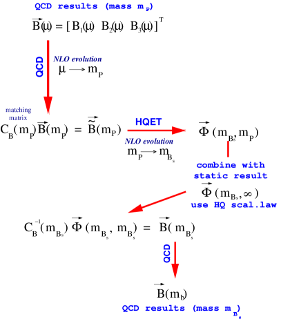
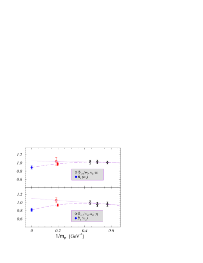
Figure 2: The procedure of matching $QCD\leftrightarrow HQET$ is sketched and the mass ‘interpolation’ illustrated. We combine the results obtained in QCD with three heavy–light mesons $m_{P}$, with the static HQET result, $m_{P}\to\infty$. The result of the linear extrapolation to $1/m_{B_{s}}$ is marked by the empty squares, whereas the “interpolation” is denoted by the filled squares. [1] and [2] are the components of the vector $\vec{\Phi}$, which are, after getting to $1/m_{B_{s}}$, matched back to the QCD parameters $B_{1,2}(m_{b})$, the results of which are given in eq. (10).

i) and ii) ensure that the final results for $B$-parameters are indeed the ones corresponding to the $\overline{\rm MS}$(NDR) scheme of ref. [9] in QCD. The schematic procedure of matching and the “interpolation” to $m_{B_{s}}$, are shown in fig. 2. We obtain the following results

$$B_{1}(m_{b})=0.87(2)(5)\;,\hskip 22.76219ptB_{2}(m_{b})=0.84(2)(4)\;,$$ (10)

where the first errors are statistical and the second include various sources of systematics. An important remark is that the above results are obtained in the quenched approximation ($n_{f}=0$), and the systematic error due to quenching could not be estimated. This year’s novelty is the research made in that direction by the JLQCD collaboration [17]. Within the NRQCD approach, they examined the effect of inclusion of the dynamical quarks. They conclude that the $B$-parameters are essentially insensitive to switching from $n_{f}=0$ to $n_{f}=2$. From their (high statistics) unquenched simulation, they quote

$$B_{1}(m_{b})=0.87(4)(7)\;,\hskip 22.76219ptB_{2}(m_{b})=0.86(3)(7)\;.$$ (11)

Notice that the two new lattice results (eqs. (10) and (11)) are in very good agreement.

1.2 Phenomenology: taking all pieces together

We can now either follow ref. [9] and write

$$\left({\Delta\Gamma\over\Gamma}\right)_{B_{s}}=\Bigl{(}5.03(32)\ {\rm GeV}^{-2}\Bigr{)}\cdot\;f_{B_{s}}^{2}B_{1}(m_{b})\;{\cal M}(m_{b})\;,$$ (12)

$${\rm where\;}\;\ {\cal M}(m_{b})=G_{1}(m_{b})-G_{2}(m_{b}){\langle\bar{B}_{s}|O_{2}(m_{b})|B_{s}\rangle\over\langle\bar{B}_{s}|O_{1}(m_{b})|B_{s}\rangle}+\delta_{1/m}\;,$$

or, as proposed in [13], we can write

$$\left({\Delta\Gamma\over\Gamma}\right)_{B_{s}}=\Bigl{(}1.09(10)\times 10^{-5}\Bigr{)}\cdot{\,\left(\tau_{B_{s}}\Delta m_{d}\right)^{\rm EXP.}\over\left|{V_{tb}V_{td}}\right|^{2}}\,\xi^{2}\,{\cal M}(m_{b})\;.$$ (13)

Indeed, by using $\xi^{2}$ and the experimental value for $\Delta m_{d}=0.519(20)(16)\ \mbox{ps}^{-1}$ [18], we avoid the multiplication by $f_{B_{s}}$, for which the uncertainty is much larger than the one for the ratio $\xi=f_{B_{s}}\sqrt{B_{1}^{(s)}}/f_{B_{d}}\sqrt{B_{1}^{(d)}}=1.15(6)$ [19], for which many of the systematic errors cancel. The critique has it that since the value for $|V_{tb}V_{td}|$ is needed to evaluate eq. (13), one has to have recourse to their values obtained from the unitarity triangle analysis [20], which implies that we assume the validity of the Standard Model (SM) [6]. I believe, however, that the assumed quark–hadron duality is more of an issue than the validity of the SM, and therefore we should rather focus our attention on testing the duality (hypothesis) within the SM (theory).

Moreover, I do not see sense in looking for the physics beyond the SM from this quantity before taming the $1/m_{b}$ corrections. To back this claim, let us use the parameters (10) and write the contributions to eq. (13) term by term

$$\left({\Delta\Gamma\over\Gamma}\right)_{B_{s}}=0.005(9)\ +\ 0.146(28)\ -\ 0.086(19)=6.5\pm 2.0^{+1.3}_{-2.1}=6.5^{+2.4}_{-2.9}\ \%\;,$$ (14)

where I also used $\delta_{1/m}=-0.5(1)$, as it can be obtained by applying the VSA to estimate the values of all the matrix elements that contribute at $1/m_{b}$ (identified in ref. [8]). The error in $\delta_{1/m}$ is an ad hoc estimate. Note that in (14) I added separately the error due to the residual scale dependence in the coefficient functions (as obtained after varying $m_{b}\leq\mu\leq 2m_{b}$). If, instead of the results (10), we take the values obtained by JLQCD (11), the final number becomes $\left({\Delta\Gamma/\Gamma}\right)_{B_{s}}=6.8^{+2.8}_{-3.4}\ \%$. So, the final values are numerically small (much below the experimental limit). From eq. (14) we also see why it is so: $1/m_{b}$ corrections are very large and are of the sign opposite w.r.t. the second term, which would otherwise dominate eq. (13). The matrix elements that are present in $\delta_{1/m}$ are very hard to compute and it will take quite some time before the lattice results for $\delta_{1/m}$ appear.

Finally, by using the same set of parameters and the results (10), plus the value $f_{B_{s}}\approx 230(30)$ MeV [19], from eq. (12) I obtain a slightly higher central value, but a result totally consistent with the above numbers, namely $\left({\Delta\Gamma/\Gamma}\right)_{B_{s}}=8.2^{+3.1}_{-5.0}\ \%$.

Before closing this part, I would like to mention ref. [21] in which it has been argued that the width difference $\left({\Delta\Gamma/\Gamma}\right)_{B_{d}}$ might be esential for the accurate determination of $\sin 2\beta$ at the LHC. For details on the theoretical estimate of that quantity please see ref. [21]. Notice that they do not include the effects of the charm quark mass in the NLO correction to the coefficient functions. A main comment, however, is that like in the case of $\left({\Delta\Gamma/\Gamma}\right)_{B_{s}}$ also in this case it is highly important to get a better control over $1/m_{b}$ corrections.

2 RATIOS OF THE $B$-MESON LIFETIMES

The hierarchy of the heavy meson lifetimes (for a given heavy quark),

$$\tau(D^{+})\ \gg\ \tau(D^{0})\ \gg\ \tau(D_{s})\;,$$ (15)

$$\tau(B^{+})\ \gtrsim\ \tau(B^{0})\ \gtrsim\ \tau(B_{s})\;,$$

can be explained by the effects of the spectator quark. Theoretically formal way of expressing that, as in the previous section, is to perform the OPE, which reduces to identifying the local operators of ${\cal O}(1/m_{b}^{3})$. Obviously, the goal is to have an accurate theoretical determination of the ratios of the $B$-meson lifetimes, confront them to the precise experimental measurements, and therefore to test the underlying assumption of quark–hadron duality. Although we are still a long way from that level of accuracy, the steady theoretical progress made over the last 10 years is rather encouraging. 

The spectator effects start showing up in OPE with the term $\propto 1/m_{b}^{3}$. Out of many $\Delta B=0$ local operators contributing at that order, only a few are expected to be relevant to the ratios $\tau(B_{u(s)})/\tau(B_{d})$. These have been identified in ref. [23], and parametrized as follows:

$$\langle B_{q}|(\bar{b}q)_{V-A}(\bar{q}b)_{V-A}|B_{q}\rangle=f_{B_{q}}^{2}m_{B_{q}}^{2}B_{1}(\mu)\,,$$ (16)

(17)

$$\langle B_{q}|\left(\bar{b}{\lambda^{i}\over 2}q\right)_{V-A}\left(\bar{q}{\lambda^{i}\over 2}b\right)_{V-A}|B_{q}\rangle=f_{B_{q}}^{2}m_{B_{q}}^{2}\varepsilon_{1}(\mu)\,,$$ (18)

(19)

$$\langle B_{q}|(\bar{b}q)_{S-P}(\bar{q}b)_{S+P}|B_{q}\rangle=f_{B_{q}}^{2}m_{B_{q}}^{2}B_{2}(\mu)\,,$$ (20)

(21)

$$\langle B_{q}|\left(\bar{b}{\lambda^{i}\over 2}q\right)_{S-P}\left(\bar{q}{\lambda^{i}\over 2}b\right)_{S+P}|B_{q}\rangle=f_{B_{q}}^{2}m_{B_{q}}^{2}\varepsilon_{2}(\mu)\,.$$ (22)

In the VSA, the colour singlet–singlet ($ss$) parameters are expected to be $B_{1}^{\rm VSA}=1$ and $B_{2}^{\rm VSA}=[m_{B_{q}}/(m_{b}+m_{q})]^{2}\approx 1.5$, whereas the octet–octet ($oo$) ones are expected to give $\varepsilon_{1,2}^{\rm VSA}=0$. The final expression for $\tau(B_{u})/\tau(B_{d})$ can be written as

$${\tau(B^{+})\over\tau(B^{0})} = 1\ +\ 16\pi^{2}{f_{B}^{2}m_{B}\over m_{b}^{3}c_{3}(m_{b})}\ \biggl{\{}\,G_{1}^{ss}(m_{b})\ B_{1}(m_{b})\ +\ G_{1}^{oo}(m_{b})\ \varepsilon_{1}(m_{b})$$ (25)

$$\hskip 88.20354pt+\ G_{2}^{ss}(m_{b})\ B_{2}(m_{b})\ +\ G_{2}^{oo}(m_{b})\ \varepsilon_{2}(m_{b})+\bar{\delta}_{1/m_{b}}\biggr{\}}\,.$$

The main ingredients in this formula are:

• $16\pi^{2}$ is the (“famous”) phase space enhancement of the spectator corrections ($\propto 1/m_{b}^{3}$);

• $c_{3}(m_{b})$ is the coefficient of the leading order term ($\propto 1/m_{b}^{0}$) which survives the cancellation of the operators $\langle B_{q}|\bar{b}b|B_{q}\rangle$ in the ratio (25). It consists of the phase space integrations in the total width of $B$-meson ($b$-quark), plus the QCD radiative corrections. The NLO computation for $c_{3}(m_{b})$ has been completed in ref. [24]. An easier way to obtain this value (see [8]) is to use the measured $b$-quark semileptonic branching fraction $B_{SL}^{\rm EXP.}=\Gamma(B\to Xe\nu)/\Gamma_{TOT}=10.6(3)\%$ [25], and combine it with the theoretical expression for $\Gamma(B\to Xe\nu)$ [26]. I obtain,

  $$c_{3}(m_{b})=3.8(1)(3)\,,$$ (26)

  where the last error comes from varying $m_{c}/m_{b}=0.30\pm 0.02$;

• $G_{1,2}(\mu)$ are the functions describing the short distance QCD dynamics of $\Delta B=0$ operators. The situation with the computation of these functions is as follows. At LO in QCD, and by neglecting the charm quark mass (i.e. $z=m_{c}^{2}/m_{b}^{2}=0$), they were first computed in ref. [27]. Inclusion of the finite charm-quark mass effects ($z\neq 0$) was made in ref. [23]. This year’s novelty is the computation of the NLO corrections. To get the final results, the authors of ref. [28] keep $z\neq 0$ in the LO term, and set $z=0$ in the NLO one. To better monitor the change in values for $G_{1,2}(\mu)$, I list all the functions needed in eq. (25), both at LO and after including the NLO QCD corrections.

  	$G_{1}^{ss}(m_{b})$	$-G_{1}^{oo}(m_{b})$	$G_{2}^{ss}(m_{b})$	$G_{2}^{oo}(m_{b})$
  LO($z=0$)	0.19	10.03	0.06	2.43
  LO($z=0.3^{2}$)	0.16	8.40	0.06	2.37
  NLO($z=0$)	0.52	9.60	0.03	1.86
  NLO($z=0.3^{2}$ and $z=0$)	0.55	8.08	0.03	1.80

  Table 1: The values of the functions $G_{i}(m_{b})$ appearing in eq. (25) as obtained in ref. [28]. The corresponding numbers relevant to the ratio $\tau(B_{s})/\tau(B_{d})$ can be found in that reference.

  Qualitatively, as in the case of $(\Delta\Gamma/\Gamma)_{B_{s}}$, the authors of ref [28] explicitly verify the infrared safety of $G^{\rm NLO}_{1,2}(\mu)$. However, they do not estimate the residual scale dependence of $G_{1,2}(m_{b})$. For the phenomenological considerations I will add (hopefully) conservative $\pm 20$% of that error. Concerning the change in value for each of the functions $G_{1,2}(m_{b})$, we see from table 1 that they all receive rather moderate radiative corrections except for the “dramatic” case of $G_{1}^{ss}(m_{b})$, whose central value changes as much as

  $${G_{1}^{ss\ \rm NLO}(m_{b})-G_{1}^{ss\ \rm LO}(m_{b})\over G_{1}^{ss\ \rm LO}(m_{b})}\simeq 2.5\;.$$ (27)

• $\bar{\delta}_{1/m_{b}}$ stands for the neglected terms $\propto 1/m_{b}^{3}$ which are not enhanced by “$16\pi^{2}$”, and for the terms in OPE that are $\propto 1/m_{b}^{4}$. A discussion of the former has been made in ref. [29], while for the latter no research has been made to date. It would be nice to follow the lines of ref. [8] and check whether the VSA indicates $\bar{\delta}_{1/m_{b}}$ to be small or large.

• Until this year, there was only one lattice study of the matrix elements (16), and that one was made in the static limit of HQET [30] (see also ref. [31]). This year, the first lattice QCD computation of $\Delta B=0$ operators has been performed [32], the main features of which will be explained in the next subsection. Besides lattice simulations, also the QCD sum rule methodology was employed in HQET to estimate the wanted bag parameters [33]. The compendium of the present results looks as follows:

  $${\underline{\rm Sum\ rules\ (HQET)}}~{}{\rm\cite[cite]{[\@@bibref{}{chung}{}{}]}}\hskip 39.83385pt{\underline{\rm Lattice\ HQET}}~{}{\rm\cite[cite]{[\@@bibref{}{massimo}{}{}]}}\hskip 45.5244pt{\underline{\rm Lattice\ QCD}}~{}{\rm\cite[cite]{[\@@bibref{}{damir2}{}{}]}}$$

  $$B_{1}(m_{b})=1.01(1)\,\hskip 64.01869ptB_{1}(m_{b})=1.06(8)\,\hskip 49.79231ptB_{1}(m_{b})=1.10(13)\left({}^{+.10}_{-.21}\right)\,$$

  $$B_{2}(m_{b})=0.99(1)\,\hskip 64.01869ptB_{2}(m_{b})=1.01(6)\,\hskip 49.79231ptB_{2}(m_{b})=0.79(5)(9)\,$$

  $$\varepsilon_{1}(m_{b})=-0.08(2)\,\hskip 59.75095pt\varepsilon_{1}(m_{b})=-0.01(3)\,\hskip 44.10185pt\varepsilon_{1}(m_{b})=-0.02(2)\left({}^{+.01}_{-.00}\right)\,$$

  $$\varepsilon_{2}(m_{b})=-0.01(3)\,\hskip 59.75095pt\varepsilon_{2}(m_{b})=-0.01(2)\,\hskip 44.10185pt\varepsilon_{2}(m_{b})=0.03(1)\left({}^{+.01}_{-.00}\right)\,$$

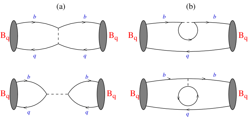
Figure 3: Graphs (a) are computed on the lattice. Graphs (b) are not. Dashed lines denote a $\Delta B=0$ four-quark operator (16).

Before updating the values for $\tau(B_{u,s})/\tau(B_{d})$, I stop here to give a few details concerning the lattice QCD computation of $\Delta B=0$ operators. The reader not interested in lattice QCD “cuisine” may skip the next subsection.

2.1 Lattice QCD estimate of $B_{1,2}(m_{b})$ and $\varepsilon_{1,2}(m_{b})$

Since the paper containing details about this computation has not been released [32], I feel it is fair to the lattice community (and wider) to explain a few elements involved in this computation. We employ the $24^{3}\times 48$ lattice at $\beta=6.2$ (i.e. $a^{-1}=2.7(1)$ GeV) and use the Wilson fermions to compute the diagrams shown in fig. 3(a). We have three values of the heavy and three values of the light quark masses. For easier orientation, our heavies are around the charm quark mass, while the lights are around the strange one. It is convenient to redefine the bag parameters for the operators as

$$B_{2}\to\overline{B}_{2}\cdot{m_{B_{q}}^{2}\over(m_{b}+m_{q})^{2}}\;,\quad\quad\varepsilon_{2}\to\overline{\varepsilon}_{2}\cdot{m_{B_{q}}^{2}\over(m_{b}+m_{q})^{2}}\;,$$ (29)

so that $\overline{B}_{2}^{VSA}=1$. To subtract the spurious mixings with other 6 dimension-six operators from the bare operators (peculiarity of the lattice computation with Wilson fermions), and to match them with the continuum ones, renormalized in the RI/MOM scheme, we used the 1-loop (boosted) perturbative expressions of ref. [34]. Since the NLO coefficients in this matching procedure are quite large it is desirable to renormalize the operators non-perturbatively and check the impact on the values presented in eq. ($\circledast$ ‣ 2). That work is in progress. The bag parameters ($B_{1}$, $\overline{B}_{2}$, $\varepsilon_{1}$, $\overline{\varepsilon}_{2}$) are extracted in the usual way, that is from the suitable ratios of the three-point and two-point correlation functions. We convert the extracted values from RI/MOM to the $\overline{\rm MS}$(NDR) renormalization scheme of ref. [35], to combine them with the coefficient functions $G_{1,2}(m_{b})$ from table 1.

The extrapolation of all the bag parameters in the light quark mass, to the physical $up/down$ quark, has been done linearly. Finally, these results are extrapolated in the inverse heavy meson mass, as shown in fig. 3. We matched the leading order anomalous dimension matrices in QCD with the ones in HQET ($\Phi(m_{P})$ in fig. 4), in such a way that the extrapolated quantity $\Phi(m_{B})$ leads directly to the desired bag parameters in QCD.

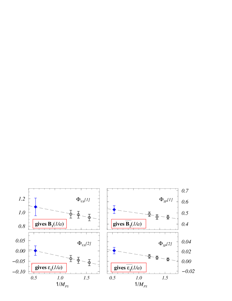
Figure 4: Extrapolation of the bag parameters of $\Delta B=0$ operators in inverse heavy meson mass (displayed in lattice units) from the masses accessible from our lattice study (empty symbols) to the $B$-meson mass (filled symbols). The plotted numbers correspond to the $\overline{\rm MS}$(NDR) scheme and $\mu=1/a=2.7(1)$ GeV.

To get the numbers given in eq. ($\circledast$ ‣ 2), we transform $\overline{B}_{2}\to B_{2}$ and $\overline{\varepsilon}_{2}\to\varepsilon_{2}$ as indicated in eq. (29). Many sources of systematic uncertainties are included in the second error in eq. ($\circledast$ ‣ 2). Please note that the parameter $B_{2}$ is quite far from its VSA value (our $B_{2}(m_{b})\approx 0.8(1)$, whereas $B_{2}^{VSA}\approx 1.5$).

2.2 Lifetime ratios: final touch

We are now ready to combine all the above results and update the theoretical prediction concerning the ratio of the heavy meson lifetimes. By using $f_{B}=0.198(30)$ GeV [19], I finally obtain

$${\tau(B^{+})\over\tau(B^{0})}\;=\;1.067(27)\;\simeq\;1.07(3)\;.$$ (30)

If we take for the bag parameters the results obtained from the lattice HQET (without the appropriate NLO matching to QCD!), we get ${\tau(B^{+})/\tau(B^{0})}=1.06(3)$.

As for the ratio ${\tau(B_{s})/\tau(B_{d})}$, I combine the NLO-corrected values for the coefficient functions [28] with the bag parameters obtained in lattice QCD ($\circledast$ ‣ 2), to arrive at

$${\tau(B_{s})\over\tau(B_{d})}\,=\,0.998(15)\,\simeq\,1.00(2)\;.$$ (31)

This result remains unchanged when the bag parameters are replaced by those determined from the lattice HQET.

2.3 Cum grano salis

In the computation of the bag parameters, we did not include the penguin-like contractions shown in fig. 3(b). The renormalization of such a diagram in QCD is very difficult, because the $\Delta B=0$ dimension-six operators may mix with the lower dimensional ones (e.g. $\bar{b}b$); we thus have to first make a power subtraction of such mixings , followed by the (standard) multiplicative renormalization. Up to now, there is no method allowing such a computation non-perturbatively. Notice that in ref. [30], the contractions from fig. 3(b) were omitted too.

A similar problem appears in perturbation theory when one computes the coefficient functions $G^{\rm NLO}_{1,2}(m_{b})$ by including penguins similar to those shown in fig. 3(b). The situation becomes even worse because, for dimensional reasons, the mixing with e.g. $\bar{b}b$ is $\propto\alpha_{s}(m_{b})m_{b}^{3}\bar{b}b$, so that the counting in the OPE breaks down. The way out is to match the QCD with the HQET, where the heavy quark is completely integrated out and the counting in $1/m_{b}$ is guaranteed from the first principles. In addition, no spurious mixings with lower dimensional operators appear in (dimensionally regularized) perturbation theory. A complete discussion of that point can be found in ref. [28].

After having made this important remark, one also needs to give a rationale for neglecting those (in)famous contractions. The argument, as presented in ref. [23], says that since these penguin-like contractions do not directly include the spectator quark effects, their presence in the ratio ${\tau(B_{u})/\tau(B_{d})}$ can be safely neglected, owing to the isospin symmetry. In other words, a given $\Delta B=0$ operator in fig. 3(b) does not feel a switch $u\leftrightarrow d$ on the spectator line, and since such contractions appear as a difference in the ratio ${\tau(B_{u})/\tau(B_{d})}$, their contributions cancel. The argument holds also for ${\tau(B_{s})/\tau(B_{d})}$, but in this case the assumption is somewhat stronger since the SU(3) light flavour symmetry has to be invoked.

Of course, this argument is not valid if one needs to estimate a combination $B_{1}(\mu)-B_{2}(\mu)$, which is relevant for the precision extraction of $|V_{ub}|$ from the inclusive semileptonic $B\to X_{u}\ell\nu_{\ell}$ decay [36]. For this study, the inclusion of the penguin-like contractions of fig. 3(b) is mandatory.

3 Summary and prospects

After several years of exciting research to reduce the theoretical uncertainty on $(\Delta\Gamma/\Gamma)_{B_{s}}$, the leading term in OPE for this quantity is in good shape: NLO perturbative corrections and quite reliable estimates of the matrix elements, obtained from new lattice studies, are available. However, a rough estimate of the subleading ($1/m_{b}$) corrections in the OPE indicates that such corrections, to a large extent, wash out the effect of the leading terms: the corrections are large and of opposite sign. Therefore, as of now, it does not seem reasonable to test the Standard Model (or to expect to see the signal of physics beyond the Standard Model) from this quantity. It is, in fact, necessary to improve the theoretical predictions by taming the dimension-seven operators (the ones that enter with $1/m_{b}$ corrections). From the present theoretical situation I conclude that

$$\left({\Delta\Gamma\over\Gamma}\right)_{B_{s}}\ =\ \left(\ 7\ \pm\ 4\ \right)\ \%\,.$$ (32)

This year, a further theoretical improvement in the lifetime ratios of the $B$-mesons has been made. QCD radiative corrections to the coefficient functions are now being calculated, and the first QCD computation of the bag parameters performed (which is complementary to the earlier lattice HQET results). Lattice predictions will certainly improve in many respects (e.g. non-perturbative renormalization will be carried out, the penguin-like contractions are likely to be included in the HQET lattice studies, unquenched simulations in HQET will become feasible,…) Note that the operators that give rise to $1/m_{b}$ corrections to the non-spectator effects in ${\tau(B_{u,s})/\tau(B_{d})}$ are yet to be identified and their effects estimated. Such a study would be very welcome. From the present theoretical information, for the ratios of the $B$-meson lifetimes I obtain

$${\tau(B^{+})\over\tau(B^{0})}\ =\ 1.07(3)\;,\hskip 34.1433pt{\tau(B_{s})\over\tau(B_{d})}\,=\,1.00(2)\;.$$ (33)

Acknowledgement

It is a pleasure to thank my friends and collaborators of refs. [13], [14] and also those of ref. [28], for sharing their insights in topics covered by this talk. Communication with S. Ryan, N. Yamada and the authors of ref. [30] is kindly acknowledged.

References

- [1] D. Abbaneo et al. [LEP, SLD, CDF], hep-ex/0009052; D. Abbaneo, hep-ex/0108030.
- [2] M. A. Shifman, hep-ph/0009131.
- [3] A. Pich, Nucl. Phys. Proc. Suppl. 98 (2001) 385, hep-ph/0012297.
- [4] R. Aleksan, A. Le Yaouanc, L. Oliver, O. Pene and J. C. Raynal, Phys. Lett. B 316 (1993) 567.
- [5] M. A. Shifman and M. B. Voloshin, Sov. J. Nucl. Phys. 47 (1988) 511.
- [6] M. Beneke and A. Lenz, J. Phys. G27 (2001) 1219, hep-ph/0012222.
- [7] U. Nierste, hep-ph/0105215.
- [8] M. Beneke, G. Buchalla and I. Dunietz, Phys. Rev. D 54 (1996) 4419, hep-ph/9605259.
- [9] M. Beneke, G. Buchalla, C. Greub, A. Lenz and U. Nierste, Phys. Lett. B 459 (1999) 631, hep-ph/9808385.
- [10] I. I. Bigi and N. G. Uraltsev, Phys. Lett. B 280 (1992) 271.
- [11] V. Gimenez and J. Reyes, Nucl. Phys. Proc. Suppl. 93 (2001) 95, hep-lat/0009007.
- [12] S. Hashimoto, K. I. Ishikawa, T. Onogi, M. Sakamoto, N. Tsutsui and N. Yamada, Phys. Rev. D 62 (2000) 114502, hep-lat/0004022.
-
[13]
D. Becirevic, D. Meloni, A. Retico, V. Gimenez, V. Lubicz and G. Martinelli,
Eur. Phys. J. C 18 (2000) 157,
hep-ph/0006135;
D. Becirevic, Nucl. Phys. Proc. Suppl. 94 (2001) 337, hep-lat/0011075. - [14] D. Becirevic, V. Gimenez, G. Martinelli, M. Papinutto and J. Reyes, hep-lat/0110091.
- [15] V. Gimenez and J. Reyes, Nucl. Phys. B 545 (1999) 576, hep-lat/9806023.
- [16] V. Gimenez and J. Reyes, “Two-loop HQET Anomalous Dimensions of all four-quark operators”, in preparation.
- [17] S. Hashimoto and N. Yamada [JLQCD collaboration], hep-ph/0104080; N. Yamada et al. [JLQCD Collaboration], hep-lat/0110087.
- [18] B. Aubert et al. [BABAR Collaboration], hep-ex/0107036.
-
[19]
C. W. Bernard,
Nucl. Phys. Proc. Suppl. 94 (2001) 159,
hep-lat/0011064;
S. Ryan, plenary talk at “Lattice 2001”. -
[20]
M. Ciuchini et al.,
JHEP 0107 (2001) 013,
hep-ph/0012308;
A. Hocker et al., Eur. Phys. J. C 21 (2001) 225, hep-ph/0104062. - [21] A. S. Dighe, T. Hurth, C. S. Kim and T. Yoshikawa, arXiv:hep-ph/0109088.
-
[22]
M. Neubert, hep-ph/9707217;
I. I. Bigi, hep-ph/0001003;
M. B. Voloshin, hep-ph/0004257. - [23] M. Neubert and C. T. Sachrajda, Nucl. Phys. B 483 (1997) 339, hep-ph/9603202.
-
[24]
E. Bagan, P. Ball, V. M. Braun and P. Gosdzinsky,
Phys. Lett. B 342 (1995) 362
[Erratum, ibid. B 374 (1995) 363], hep-ph/9409440,
E. Bagan, P. Ball, B. Fiol and P. Gosdzinsky, Phys. Lett. B 351 (1995) 546, hep-ph/9502338. - [25] C. S. Lin, hep-ex/0105025.
- [26] Y. Nir, Phys. Lett. B 221 (1989) 184.
- [27] I. I. Bigi, hep-ph/9508408.
- [28] M. Ciuchini, E. Franco, V. Lubicz and F. Mescia, hep-ph/0110375.
- [29] D. Pirjol and N. Uraltsev, Phys. Rev. D 59 (1999) 034012, hep-ph/9805488.
- [30] M. Di Pierro and C. T. Sachrajda, Nucl. Phys. B 534 (1998) 373, hep-lat/9805028.
- [31] J. Flynn and C. J. Lin, J. Phys. G G27 (2001) 1245, hep-ph/0012154.
- [32] D. Becirevic et al., “B-meson lifetime ratios: Lattice QCD estimate of operators”, in preparation.
- [33] M. S. Baek, J. Lee, C. Liu and H. S. Song, Phys. Rev. D 57 (1998) 4091, hep-ph/9709386.
- [34] R. Gupta, T. Bhattacharya and S. R. Sharpe, Phys. Rev. D 55 (1997) 4036, hep-lat/9611023.
-
[35]
A. J. Buras, M. Misiak and J. Urban,
Nucl. Phys. B 586 (2000) 397,
hep-ph/0005183;
M. Ciuchini, E. Franco, V. Lubicz, G. Martinelli, I. Scimemi and L. Silvestrini, Nucl. Phys. B 523 (1998) 501, hep-ph/9711402. - [36] M. B. Voloshin, Phys. Lett. B 515 (2001) 74, hep-ph/0106040.