Error Estimates on Parton Density Distributions

Abstract

Error estimates on parton density distributions are presently based on the traditional method of least squares minimisation and linear error propagation in global QCD fits. We review the underlying assumptions and the various mathematical representations of the method and address some technical issues encountered in such a global analysis. Parton distribution sets which contain error information are described.

1 Introduction

Parton density distributions are important ingredients in the calculation of hard scattering lepton-hadron and hadron-hadron cross sections. To judge the comparison of theory and experiment it is important to evaluate the experimental and theoretical uncertainties on the predicted cross sections which are often dominated by those on the input parton densities. These densities are non-perturbative and are obtained from QCD fits to a large body of scattering data. The errors which have to be propagated in such a fit are the statistical and correlated systematic errors on the measurements, errors on the input parameters (flavour thresholds, $\alpha_{s}$ etc.) and uncertainties in the theoretical modelling (scale errors, non-perturbative contributions like higher twists and nuclear effects, functional form of the parton densities and so on).

In the past the errors associated with the parton densities were often determined from the spread between different parton distribution sets. Such a spread is of course by no means a representation of the experimental and theoretical uncertainty. In recent years considerable progress is made on the proper error propagation in global QCD fits because the increasing accuracy of the HERA and Tevatron data demands reliable estimates of the uncertainties in the theory predictions. Parton density uncertainties are of course also important for the ongoing LHC simulation studies.

Two methods of error propagation are presently in use. One is based on the method of statistical inference using Monte Carlo integration techniques [1]. The more conventional approach makes use of the standard methods of least squares minimisation and linear error propagation. In this report we will restrict ourselves to a description of the latter method because it is, at present, the most developed and widely used in QCD fits by the various experimental collaborations and theory groups.

2 Least Squares Minimisation

The justification for using least squares lies in the assumption that the measurement errors are Gaussian distributed. To introduce the effect of point to point correlated systematic errors, the measurements ($\bi{m}$) are related to the theory prediction ($\bi{t}$) by

$$m_{i}=t_{i}(\bi{p})+r_{i}\sigma_{i}+\sum_{k}s_{k}\Delta_{ik}$$ (1)

where $m_{i}$ is the measurement of data point $i$, $t_{i}(\bi{p})$ is the model prediction depending on a set of parameters $\bi{p}$, $\sigma_{i}$ is the uncorrelated (statistical) error on data point $i$ and $\Delta_{ik}$ is the correlated (systematic) error from source $k$.

In (1), $r_{i}$ and $s_{k}$ denote Gaussian random variables with zero mean and unit variance. These random variables are assumed to be independent of each other:

$$\langle\Delta r_{i}\Delta r_{j}\rangle=\langle\Delta s_{i}\Delta s_{j}\rangle=\delta_{ij}\qquad\langle\Delta r_{i}\Delta s_{j}\rangle=0$$ (2)

where we have introduced the notation $\Delta x=x-\langle x\rangle$ and where the symbol $\langle\ \rangle$ denotes an average. The probability density function of the measurements can then be written as a multivariate Gaussian distribution

$$P=C\exp(-{\textstyle\frac{1}{2}}\chi^{2})$$ (3)

with $C$ a normalisation constant and $\chi^{2}$ defined by

$$\chi^{2}=\sum_{ij}(m_{i}-t_{i})V_{ij}^{-1}(m_{j}-t_{j}).$$ (4)

From (1) and (2) the covariance matrix $\bi{V}$ of the measurements is given by

$$V_{ij}=\langle\Delta m_{i}\Delta m_{j}\rangle=\delta_{ij}\sigma_{i}^{2}+\sum_{k}\Delta_{ik}\Delta_{jk}.$$ (5)

Optimal values for the parameters, $\bi{p}_{0}$, are found by maximising the probability density $P$ or, equivalently, by minimising $\chi^{2}$ defined by (4).

The standard method to calculate the covariance matrix of the fitted parameters is based on the assumption that the theory prediction varies approximately linearly with $\bi{p}$ near the minimum of $\chi^{2}$ at $\bi{p}_{0}$. Expanding $\chi^{2}$ up to second order in the variation $\Delta\bi{p}=\bi{p}-\bi{p}_{0}$ gives

$$\Delta\chi^{2}=\chi^{2}(\bi{p})-\chi^{2}(\bi{p}_{0})=\sum_{i}\frac{\partial\chi^{2}}{\partial p_{i}}\;\Delta p_{i}+\sum_{ij}\frac{1}{2}\frac{\partial^{2}\chi^{2}}{\partial p_{i}\partial p_{j}}\;\Delta p_{i}\Delta p_{j}.$$ (6)

Because the linear term in (6) vanishes at the minimum we find for the covariance matrix $\bi{V}_{p}$ of the parameters

$$V_{ij}^{p}=\langle\Delta p_{i}\Delta p_{j}\rangle=\Delta\chi^{2}\left(\frac{1}{2}\frac{\partial^{2}\chi^{2}}{\partial p_{i}\partial p_{j}}\right)^{-1}=\Delta\chi^{2}\;H^{-1}_{ij}$$ (7)

where we have introduced the Hessian matrix $\bi{H}$ of second order derivatives. Notice that the covariance matrix $\bi{V}_{p}$ depends on the choice of $\Delta\chi^{2}$ which usually, but not always, is taken to be $\Delta\chi^{2}=1$. With this choice the probability density given in (3) drops by a factor $\sqrt{e}$ when the parameters $\bi{p}$ are a distance $\Delta\bi{p}$ away from the optimum. This corresponds to the definition of the width of a Gaussian distribution.

Having obtained the best values and the covariance matrix of the parameters, the covariance of any two functions $F(\bi{p})$ and $G(\bi{p})$ can be calculated with the standard formula for linear error propagation

$$\langle\Delta F\Delta G\rangle=\sum_{ij}\frac{\partial F}{\partial p_{i}}\;V_{ij}^{p}\;\frac{\partial G}{\partial p_{j}}=\Delta\chi^{2}\sum_{ij}\frac{\partial F}{\partial p_{i}}\;H_{ij}^{-1}\;\frac{\partial G}{\partial p_{j}}.$$ (8)

Here it is assumed that both $F$ and $G$ vary approximately linearly with $\bi{p}$ in the neighbourhood of $\bi{p}_{0}$. Because $\langle\Delta F^{2}\rangle>0$ it follows from (8) that the Hessian (and its inverse) must be positive definite, that is, for arbitrary vectors $\bi{X}$,

$$\bi{XHX}>0.$$ (9)

Finally we remark that, for simplicity, we have tacitly assumed that all errors can be treated as offsets. Notice that multiplicative (normalisation) errors must be treated somewhat differently [2] to avoid possible large biases in the fit results [3].

3 The Hessian Matrix

In the quadratic approximation (6) a constant value of $\Delta\chi^{2}$ traces out an ellipsoid in parameter space as illustrated in figure 1a.

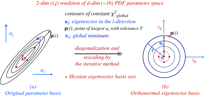
Figure 1: (a) Ellipsoid contours defined by constant values of $\chi^{2}$ in parameter space. (b) Hyper-sphere contours of constant $\chi^{2}$ after an orthogonal transformation of the parameters defined by the eigenvectors and eigenvalues of the Hessian matrix. Figure taken from [4].

When the directions of the major axes of this ellipsoid coincide with the directions of the parameter coordinate system the Hessian matrix is diagonal and the parameters are said to be uncorrelated. If this is not the case the Hessian can be made diagonal by a coordinate transformation to the major axes, that is, by a rotation in parameter space around the centre $\bi{p}_{0}$ of the ellipsoid. This transformation can be written as

$$\Delta y_{i}=\sum_{j}U_{ij}\;\Delta p_{j}\qquad\sum_{i}U_{ij}\;U_{ik}=\delta_{jk}$$ (10)

where the second equation states that $\bi{U}$ is an orthonormal transformation (rotation). The matrix $\bi{U}$ is given by the complete set of eigenvectors of the Hessian matrix as defined by the eigenvalue equation

$$\sum_{j}H_{ij}\;U_{kj}=\epsilon_{k}\;U_{ki}.$$ (11)

The errors on the transformed parameters $y_{i}$ are given by $1/\sqrt{\epsilon}_{i}$ so that all eigenvalues of $\bi{H}$ must be positive, which is another way to state that the Hessian is positive definite. We mention at this point that a non-positive definite Hessian encountered in a (QCD) fit is a sign of either numerical problems in the calculation of $\chi^{2}$ (no smooth behaviour around the minimum) or of large correlations between the fitted parameters ($\bi{H}$ cannot be inverted). In the latter case one or more parameters should be kept fixed in the fit or a different parameterisation of the theory prediction should be considered.

Rescaling $z_{i}=y_{i}\sqrt{\epsilon}_{i}$ maps the ellipsoid on a hyper-sphere in $z$-space as indicated in figure 1b. Notice that if $F$ and $G$ are given as functions of $\bi{y}$ or $\bi{z}$, instead of $\bi{p}$, equation (8) transforms to the expression

$$\langle\Delta F\Delta G\rangle=\Delta\chi^{2}\sum_{i}\frac{\partial F(\bi{y})}{\partial y_{i}}\;\frac{1}{\epsilon_{i}}\;\frac{\partial G(\bi{y})}{\partial y_{i}}=\Delta\chi^{2}\sum_{i}\frac{\partial F(\bi{z})}{\partial z_{i}}\;\frac{\partial G(\bi{z})}{\partial z_{i}}$$ (12)

which is of course easier to compute than (8) and, perhaps, is also numerically more accurate.

The spectrum of eigenvalues obtained from a typical QCD fit [4] is shown in the left-hand plot of figure 2.

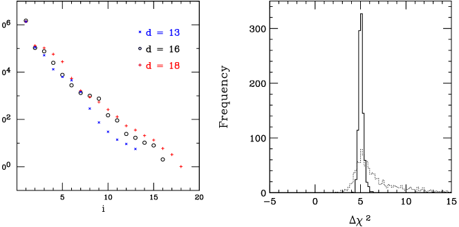
Figure 2: Left: The eigenvalue spectrum of the Hessian matrix from a typical global QCD fit with (13,16,18) free parameters. Taken from [4]. Right: Distribution of $\Delta\chi^{2}$ calculated by minuit (dashed histogram) and by an improved calculation from [6] (full histogram) on a 10-dimensional ellipsoid defined by $\Delta\chi^{2}=5$. The spread is caused by numerical errors in the calculation of the Hessian matrix.

Large (small) values of $\epsilon_{i}$ correspond to an accurate (inaccurate) determination of the transformed parameters $y_{i}$ by the fit. The large range in eigenvalues ($\approx 10^{6}$) implies that the numerical calculation of the Hessian matrix must be carried out with due attention to rounding errors. This is illustrated in the right-hand plot of figure 2 which shows the distribution of $\Delta\chi^{2}$ calculated from the Hessian by minuit [5] (dashed histogram) and by an improved algorithm [6] (full histogram) for parameter values randomly distributed on the hyper-surface $\Delta\chi^{2}=5$. The improvement in the calculation of the Hessian is achieved by using more sample points than minuit in the evaluation of the second derivatives. The algorithm is included in an update of the minuit code which can be obtained from the authors of [6].

4 Calculation of $\bi{\chi^{2}}$

Minimising $\chi^{2}$ defined by (4) is impractical because it involves the inversion of the measurement covariance matrix (5) which, in global fits, tends to become very large. Because the systematic errors of different data sets are in general uncorrelated (but not always, see [7]) this matrix takes a block diagonal form and each block could, in principle, be inverted once and for all. However, the dimension of these block matrices can still easily be larger than a few hundred. Furthermore, if the systematic errors dominate, the covariance matrix might, numerically, be uncomfortably close to a matrix with the simple structure $V_{ij}=\Delta_{i}\Delta_{j}$, which is singular.

Fortunately, the $\chi^{2}$ of (4) can be cast in an alternative form which avoids the inversion of large matrices (we refer to [8] for a derivation):

$$\eqalign{\chi^{2}&=\sum_{i}\left(\frac{m_{i}-t_{i}}{\sigma_{i}}\right)^{2}-\bi{B}\;\bi{A}^{-1}\;\bi{B}\\ B_{k}&=\sum_{i}\Delta_{ik}(m_{i}-t_{i})/\sigma_{i}^{2}\\ A_{kl}&=\delta_{kl}+\sum_{i}\Delta_{ik}\Delta_{il}/\sigma_{i}^{2}.}$$ (13)

The matrix $\bi{A}$ in (13) has the dimension of the number of systematic sources only and can be inverted at the initialisation phase of a fitting program once the number of data points included in the fit (i.e. after cuts) is known. An example of a global QCD fit with error calculations based on the covariance matrix approach can be found in [9].

It is remarkable that minimising (13) is equivalent to a fit where both the parameters $\bi{p}$ and $\bi{s}$ are left free. In such a fit $\chi^{2}$ is defined as follows. First, the effect of the systematic errors is incorporated in the model prediction

$$f_{i}(\bi{p},\bi{s})=t_{i}(\bi{p})+\sum_{k}s_{k}\Delta_{ik}.$$ (14)

Next, $\chi^{2}$ is defined by

$$\chi^{2}=\sum_{i}\left(\frac{m_{i}-f_{i}(\bi{p},\bi{s})}{\sigma_{i}}\right)^{2}+\sum_{k}s_{k}^{2}.$$ (15)

The second term in (15) serves to constrain the fitted values of $\bi{s}$. The presence of this term is easily understood if one takes the view that the calibration of each experiment yields a set of ‘measurements’ $s_{k}=0\pm 1$ [2].

Because $f$ is linear in $\bi{s}$ the minimisation with respect to the systematic parameters can be done analytically. It is easy to show, by solving the equations $\partial\chi^{2}/\partial ds_{k}=0$, that this leads to the $\chi^{2}$ given by (13) which, in turn, is equivalent to (4), see [8]. The relation between the optimal values of $\bi{s}$, the matrix $\bi{A}$ and the vector $\bi{B}$ of (13) is

$$\bi{s}=\bi{A}^{-1}\bi{B}.$$ (16)

A recent QCD analysis by the H1 collaboration [10] is based on a minimisation of (15) with the systematic parameters left free in the fit.

In the following we will use the term ‘Hessian method’ to refer to QCD fits based on the minimisation of the $\chi^{2}$ defined by (13) or (15), the alternative being the ‘offset method’ which we will describe in the next section.

5 Offset Method

There is another method to propagate the systematic errors which also has the property that the inversion of a large measurement covariance matrix is avoided. Like in the previous section $\chi^{2}$ is defined by (14) and (15) but now the systematic parameters are kept fixed to $\bi{s}=0$ in the fit. This results in minimising

$$\chi^{2}=\sum_{i}\left(\frac{m_{i}-t_{i}(\bi{p})}{\sigma_{i}}\right)^{2}$$ (17)

where only statistical errors are taken into account to get the best value $\bi{p}_{0}$ of the parameters. Because systematic errors are ignored in the $\chi^{2}$ such a fit forces the theory prediction to be as close as possible to the data.

The systematic errors on $\bi{p}$ are estimated from fits where each systematic parameter $s_{k}$ is offset by its assumed error ($\pm 1$) after which the resulting deviations $\Delta\bi{p}$ are added in quadrature. To first order this lengthy procedure can be replaced by a calculation of two Hessian matrices $\bi{M}$ and $\bi{C}$

$$M_{ij}=\frac{1}{2}\frac{\partial^{2}\chi^{2}}{\partial p_{i}\partial p_{j}}\qquad C_{ij}=\frac{1}{2}\frac{\partial^{2}\chi^{2}}{\partial p_{i}\partial s_{j}}.$$ (18)

The statistical covariance matrix of the fitted parameters is then given by

$$\bi{V}_{\rm stat}=\bi{M}^{-1}$$ (19)

while a systematic covariance matrix can be defined by [11]

$$\bi{V}_{\rm syst}=\bi{M}^{-1}\bi{CC}^{T}\bi{M}^{-1}$$ (20)

where $\bi{C}^{T}$ is the transpose of $\bi{C}$. The total covariance matrix $\bi{V}_{p}$ is given by the sum of the matrices $\bi{V}_{\rm stat}$ and $\bi{V}_{\rm syst}$.

Comparing equations (13) or (15) and (17) it is clear that the parameter values obtained by the Hessian and offset methods will, in general, be different. This difference is accounted for by the difference in the error estimates, those of the offset method being larger in most cases. In statistical language this means that the parameter estimation of the offset method is not efficient. The offset method has a further disadvantage that the goodness of fit cannot be judged from the $\chi^{2}$ which is calculated from statistical errors only. An ad hoc solution to this problem is to re-calculate, after the fit has converged, a $\chi^{2}$ with the statistical and systematic errors added in quadrature [12].

For a detailed comparison of the Hessian and offset methods we refer to [13] where it is shown that the error estimates from the two methods can differ by a large amount when the systematic errors dominate. This is illustrated in figure 3 which shows the error bands on the gluon density obtained from a LO QCD fit to the BCDMS data.

Figure 3: The gluon density versus the Bjorken scaling variable $x$ from a LO QCD fit to the BCDMS structure function data. The dotted curves show the statistical error band. The full curves indicate the systematic error band calculated using the offset method (a) and the Hessian method (b). Figure taken from [13].

This might also explain the difference in the error estimates on $\alpha_{s}$ from recent QCD fits by H1 [10] (Hessian method with free systematic parameters) and ZEUS [14] (offset method):

$$\alpha_{s}(M_{Z}^{2})=\left\{\begin{array}[]{ll}0.1150\pm 0.0017\ {\rm(exp.)}&{\rm H1}\\ 0.1172\pm 0.0055\ {\rm(exp.)}&{\rm ZEUS\ preliminary.}\end{array}\right.$$

Notice however that these fits differ in many other respects like the data sets included, kinematic cuts, treatment of charm mass effects and so on.

6 Exploring the $\bi{\chi^{2}}$ Profile

As mentioned above, the Hessian method is based on the assumption that the theory prediction is approximately linear in the vicinity of $\bi{p}_{0}$ which means that $\chi^{2}$ is a quadratic function of the parameters near the minimum. To check this quadratic dependence one can fix a parameter $p_{i}$, say, and optimise the remaining parameters for different input values of $p_{i}$. In this way $\chi^{2}$ is explored along the axes of the parameter coordinate system. The procedure is automatically carried out using the ‘Minos’ option in minuit.

The Lagrange multiplier method, developed in [8], allows to investigate the $\chi^{2}$ profile along any relevant direction in parameter space. Here the quantity

$$\chi^{2}(\bi{p},\lambda)=\chi^{2}_{g}(\bi{p})+\lambda X(\bi{p})$$ (21)

is minimised for several fixed values of the Lagrange multiplier $\lambda$. In (21) $\chi^{2}_{g}$ is the global $\chi^{2}$ calculated from the data included in the fit and $X$ is a physics quantity of interest (not included in the fit), for instance, the $W$ production cross-section $\sigma_{W}$ in $p\bar{p}$ collisions at the Tevatron. The results of such a lengthy analysis obtains the $\chi^{2}$ profile as a function of $X$ and thus the range of $X$ corresponding to a given value of $\Delta\chi^{2}$. This method does not make use of a quadratic approximation of the $\chi^{2}$ profile.

In the left-hand plot of figure 4 we show $\chi^{2}$ as function of $\sigma_{W}$ from the analysis of [8].

Figure 4: Left: The $\chi^{2}_{g}$ (see text) versus the cross-section $\sigma_{W}$ of inclusive $W$ production at Tevatron energies from the QCD analysis of [8]. Right: Optimal values of $\sigma_{W}$ (dots) and 90% confidence levels (bars) for each data set included in the fit. The full line shows the best prediction for $\sigma_{W}$ and the dashed lines represent the confidence bounds described in the text. Figures taken from [8].

In this analysis the 90% confidence levels of $\sigma_{W}$ were obtained from the $\chi^{2}$ profiles of each data set individually, see the right-hand plot of figure 4. The uncertainty on $\sigma_{W}$ was then defined as the intersection of these individual confidence levels (dashed lines in figure 4) giving $20.9<\sigma_{W}<22.6$ nb. A similar uncertainty of 4% on the $\sigma_{W}$ prediction is obtained from the Hessian method provided $\Delta\chi^{2}$ in (7) or (8) is set to 180 (for a fit of 1295 data points distributed over 15 data sets).

The origin of this large $\Delta\chi^{2}$ is unclear to us but the question which value of $\Delta\chi^{2}$ should be chosen in a global QCD analysis and which deviations from the expected $\chi^{2}$ value ($N\pm\sqrt{2N}$ for a fit with $N$ degrees of freedom) can be tolerated is clearly an important issue. For a discussion on this subject we refer to [15].

A bad $\chi^{2}$ in a global analysis may have several causes. First, it can be an indication of physics beyond the Standard Model. Second, the theoretical modelling may be inadequate because higher order terms in the perturbative expansion are missing or non-perturbative contributions like higher twists or nuclear effects are not, or only partially, taken into account. In addition, there is always the question if the parton densities are parameterised with sufficient flexibility. Third, the information on the experimental errors may be inaccurate, incomplete (not all correlations given) or even not be fully known. Finally, the data may very well not be Gaussian distributed.

Concerning the latter point we refer to an analysis [16] of a large sample of data from the Table of Particle Properties. It turns out that the probability distribution of this body of data is far from Gaussian. This may be due to uncertainties in the error estimates provided by the experiments which, as is shown in [16], can strongly affect the shape of the probability distribution of the data.

7 Parton Distribution Sets

Error calculations in global QCD fits are of little practical use if the results are not made available in the form of parton distribution sets which contain the full information on uncertainties and correlations. To our knowledge two such sets exist at present.

The set provided by Alekhin [9] gives as a function of $x$ and $Q^{2}$ the values of the parton densities and their covariance matrix as calculated with (8). This allows to compute the error on any function of the parton distributions but only at a given kinematic point. It is, for instance, not possible to evaluate the errors on (convolution) integrals since the information on the correlation between different kinematic points is lost. Notice that the errors from [9] are defined by the Hessian Method described in section 4.

The epdflib set [17] based on the QCD analysis of [12] gives the covariance matrix of the fitted parameters (from the offset method described in section 5) and, as functions of $x$ and $Q^{2}$, the parton densities as well as their derivatives to all the fitted parameters. From this information the error on any function of the parton densities can be calculated with (8). As an example let us consider a hadron-hadron cross section which can be written as a convolution of the parton densities and a hard scattering cross section, generically,

$$\sigma=\sum_{ij}f_{i}\otimes f_{j}\otimes\hat{\sigma}_{ij}.$$ (22)

To calculate the error on $\sigma$ with (8) it is sufficient to compute the derivatives

$$\frac{\partial\sigma}{\partial p_{\lambda}}=\sum_{ij}\left[\frac{\partial f_{i}}{\partial p_{\lambda}}\otimes f_{j}+f_{i}\otimes\frac{\partial f_{j}}{\partial p_{\lambda}}\right]\otimes\hat{\sigma}_{ij}$$ (23)

which is straight forward since both $f_{i}$ and the derivatives are available from epdflib. A practical example of the use of epdflib in an analysis of dijet production at HERA can be found in [18].

In figure 5 we show the parton densities from epdflib (left hand plot) and the relative error contributions to the gluon and singlet quark densities (right hand plot).

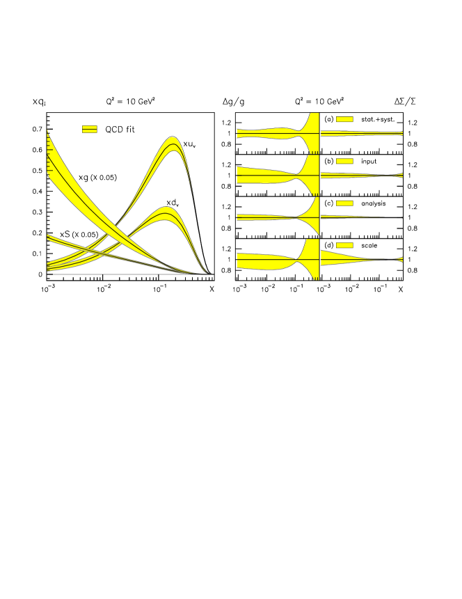
Figure 5: Left: The parton momentum densities from the QCD analysis of [12] versus $x$ at $Q^{2}=10$ GeV². Right: The errors on the gluon and quark densities from the various sources described in the text. Figures taken from [12].

The epdflib set provides, in addition to the experimental statistical and systematic errors, information on the following sources of uncertainty:

• Uncertainties due to those on the input parameters of the analysis like $\alpha_{s}$, heavy flavour thresholds, nuclear effects and so on. Parton densities are provided with each of these input parameters offset by their errors. These densities can be used to either define an error band or to obtain, by interpolation, densities with varying input conditions;

• Analysis error defined as the envelope of the central fit and 10 alternative fits (vary cuts, input scale etc.) which all gave acceptable values of $\chi^{2}$. This error band quantifies the stability of the QCD fit;

• Parton densities obtained from fits where the renormalisation and factorisation scales were independently varied in the range $Q^{2}/2<\mu^{2}_{R,F}<2Q^{2}$. Again, these densities can be used to define an error band or be interpolated to obtain the distributions for a particular choice of scale.

A simple but important check is provided by the calculation of the uncertainty on the total momentum fraction carried by quarks and gluons. This error should vanish because the momentum sum was constrained to unity in the analysis of [12]. Indeed we find with epdflib for the values and errors of these momentum fractions at $Q^{2}=4$ GeV²

$$\int_{0.001}^{1}xg\,dx\hskip 36.98857pt = 0.393\pm 0.018\ \ \mathrm{(stat.+syst.)}$$

$$\int_{0.001}^{1}x\Sigma\,dx\hskip 34.1433pt = 0.594\pm 0.018$$

$$\int_{0.001}^{1}(xg+x\Sigma)\,dx = 0.987\pm 0.002$$

where the error on the last integral is much smaller than that on the first two, as it should be. This example clearly illustrates the importance of taking into account the correlations between the errors on the parton densities.

8 Summary

In this report we have presented an overview of the least squares minimisation and error propagation techniques used in many recent global QCD fits. The aim of these global analyses is to determine from a large and diverse body of scattering data the parton density distributions as well as their errors and correlations.

Assuming that the measurement errors are Gaussian distributed the likelihood function can be written as a multivariate Gaussian distribution. This leads to a $\chi^{2}$ definition which can have different, but mathematically equivalent representations. In particular it turns out that a fit using the full covariance matrix of the data is equivalent to a fit where the systematic correlations are included in the model prediction together with the introduction of a set of free systematic parameters.

Error propagation based on shifting the data by the systematic errors and adding the deviations in quadrature is not equivalent to the method described above and leads to theory predictions which are as close as possible to the fitted data at the expense of larger error estimates, in particular when the systematic uncertainties dominate.

Several technical issues are addressed such as the numerical accuracy of the calculation of the Hessian matrix, the Lagrange multiplier method to explore the multi-dimensional $\chi^{2}$ profile in some physically relevant direction and the representation of the global QCD fit results in publically available parton distribution sets which contain the full information on errors and correlations.

I am grateful to D. Stump for providing me with mathematical proofs of the equivalence of several $\chi^{2}$ representations and to S. Alekhin, J. Pumplin, W.K. Tung and A. Vogt for discussions and comments on the manuscript. I thank the organisers for inviting me to an excellent and stimulating workshop.

references

references

- [1] Giele W T and Keller S 1998 Phys. Rev. D58 094023 (hep-ph/9803393)
- [2] D’Agostini G 1994 Nucl. Instr. Meth. A346 306
- [3] Takeuchi T 1996 Prog. Theor. Phys. Suppl. 123 247 (hep-ph/9603415)
- [4] Pumplin J et al 2001 Preprint hep-ph/0101032
- [5] James F and Roos M 1975 Comput. Phys. Comm. 10 343
- [6] Pumplin J et al 2000 Preprint hep-ph/0008191
- [7] NMC Arneodo M et al 1997 Nucl. Phys. B483 3 (hep-ph/9610231)
- [8] Stump D et al 2001 Preprint hep-ph/0101051
- [9] Alekhin S I 2001 Phys. Rev. D63 094022 (hep-ph/0011002)
- [10] H1 Collab. Adloff C et al 2001 Eur. Phys. J. C21 33 (hep-ex/0012053)
- [11] Pascaud C and Zomer F 1995 Preprint LAL-95-05
- [12] Botje M 2000 Eur. Phys. J. C14 285 (hep-ph/9912439)
- [13] Alekhin S I 2000 Preprint hep-ex/0005042
- [14] Nagano K 2001 Presented at DIS2001, Bologna, Italy, April 27–May 1 2001
- [15] Collins J C and Pumplin J 2001 Preprint hep-ph/0105207
- [16] Bukhvostov A P 1997 Preprint hep-ph/9705387
- [17] Botje M 1999 Preprint NIKHEF-99-034
- [18] Zeus Collab. Breitweg J et al 2001 Phys. Lett. B507 70 (hep-ex/0102042)