Instanton–Like Processes in Particle Collisions: a Numerical Study of the $SU(2)$-Higgs Theory below the Sphaleron Energy.

Abstract

We use semiclassical methods to calculate the probability of inducing a change of topology via a high-energy collision in the $SU(2)$-Higgs theory. This probability is determined by a complex solution to a classical boundary value problem on a contour in the complex time plane. In the case of small particle number it is the probability of instanton-like processes in particle collisions. We obtain numerically configurations with the correct topological features and expected properties in the complex time plane. Our work demonstrates the feasibility of the numerical approach to the calculation of instanton-like processes in gauge theories. We present our preliminary results for the suppression factor of topology changing processes, which cover a wide range of incoming particle numbers and energies below the sphaleron energy.

1 Introduction and Summary

Non-perturbative effects occur in many processes studied by quantum field theory. Well known examples are the decay of the false vacuum in scalar models and instanton-like transitions in gauge theories. The latter are accompanied by non-conservation of fermion quantum numbers [1], such as baryon number, and thus are of importance for particle physics and cosmology.

In weakly coupled theories, these processes are described at low energies by classical Euclidean solutions interpolating between initial and final states separated by an energy barrier. In the examples mentioned above such solutions are known as bounce [2] and instanton [3]. The Euclidean action of the solution determines the exponential part of the transition rate. It is inversely proportional to a small coupling constant present in the model and thus, in general, the rate is highly suppressed.

At energies comparable to the height of the barrier, the probabilities of the transitions between topologically distinct vacua may become unsuppressed. This takes place, for example, at finite temperature [4, 5, 6], finite fermion density [7, 8, 9], or in the presence of heavy fermions in the initial state [10, 11, 12]. In high energy particle collisions the situation is not quite the same.

As was first noted in [13, 14], at relatively low energies the corrections to the tunneling rate can be calculated by perturbative expansion in the background of the instanton (bounce). Further studies showed that the actual expansion parameter is $\varepsilon=E/E_{\mathrm{sph}}$ [15, 16, 17, 18] and the total cross section of induced tunneling has an exponential form

$$\sigma_{tot}(E)\sim\exp\left\{-\frac{16\pi^{2}}{g^{2}}F_{HG}(E/E_{\mathrm{sph}})\right\},$$

where $g$ is the small coupling constant and the function $F_{HG}(\varepsilon)$ is a series in powers of $\varepsilon\equiv E/E_{\mathrm{sph}}$ (for a review see [19]).

While the perturbation theory in $\varepsilon$ is limited to small $\varepsilon$, the general form of the total cross section implies that there might exist a semiclassical-type procedure which would allow, at least in principle, to calculate $F_{HG}(\varepsilon)$ at $\varepsilon\gtrsim 1$. Since the initial state of two highly energetic particles is not semiclassical, the standard semiclassical procedure does not apply and a proper generalization is needed, which was proposed in refs. [20, 21, 22]. The corresponding formalism reduces the calculation of the exponential suppression factor to a certain classical boundary value problem, whose analytical solution is not usually possible.

The semiclassical approach proposed in refs. [20, 21, 22] is based on the conjecture that, with exponential accuracy, the two-particle initial state can be substituted by a multiparticle one provided that the number of particles is not parametrically large. The few-particle initial state, in turn, can be considered as a limiting case of truly multiparticle one with the number of particles $N=\nu/g^{2}$ when the parameter $\nu$ is sent to zero. For the multiparticle initial state the transition rate is explicitly semiclassical and has the form

$$\sigma(E,N)\sim\exp\left\{-\frac{16\pi^{2}}{g^{2}}F(\varepsilon,\nu)\right\}.$$

According to the above conjecture, the function $F_{HG}(\varepsilon)$, corresponding to the two-particle incoming state, is reproduced in the limit $\nu\to 0$,

$$\lim\limits_{\nu\to 0}F(\varepsilon,\nu)=F_{HG}(\varepsilon).$$

Therefore, although indirectly, the function $F_{HG}(\varepsilon)$ is also calculable semiclassically. Although not proven rigorously, this conjecture was checked explicitly in field theory models in several orders of perturbation theory in $\varepsilon$ [23] and also in a quantum-mechanical model for all $\varepsilon$ [24].

Until now the only analyses of induced tunneling have been performed in a quantum mechanical model [24] and in a scalar field model of false vacuum decay [25]. A particularly interesting case to study is, however, the Electroweak Theory where different topological sectors are separated by a potential barrier of the height $E_{\mathrm{sph}}\sim 10\mathrm{TeV}$ [26, 27]. Whether the exponential suppression disappears in this theory at sufficiently high energy is still an open question. In this paper we consider an $SU(2)$ gauge theory with Higgs doublet, which corresponds to the Electroweak sector of the Standard Model with $\theta_{W}=0$.

Classically allowed over-barrier sphaleron transitions in this model were studied in ref. [28]. All solutions found in ref. [28] are configurations with large number of particles in the initial state and thus they do not correspond to few-particle collisions.

In the present work we adapt the prescription of [20, 21, 22] to theories with gauge degrees of freedom. The prescription requires the solution of field equations on a contour in complex time plane (see figure 1) with boundary conditions of a special form. Since the solutions cannot be found analytically, one has to invoke numerical techniques. Here we present solutions to this problem in a limited region of parameters. Our solutions possess all expected features, including correct topological structure and singularity structure in complex time plane. Thus, our results appear to validate the use of numerical methods for the study of instanton-like transitions in gauge theories at high energies.

In this work we explore the region of parameters with $E<E_{\mathrm{sph}}$ and $0.4\lesssim\nu<1$. We calculate the exponent of the suppression factors for a wide range of values of $E$ and $\nu$ within the above region. Not surprisingly, since we work at energies below the sphaleron energy, we find that topology changing processes remain exponentially suppressed throughout the region we studied. More relevant may be the fact that the trend of our results appears to indicate that topology changing processes with low initial particle number may remain suppressed well above $E_{\mathrm{sph}}$.

The paper is organized as follows. In section 2 we briefly review the boundary value problem for the semiclassical calculation of $\sigma(E,N)$. In section 3 we present the $SU(2)$ model used in our calculations. In section 4 we describe our numerical results and section 5 contains a few concluding remarks.

2 Semiclassical approach to induced tunneling probability

The inclusive multiparticle probability of a transition from a state with fixed energy $E$ and number of particles $N$ about one vacuum to any state about another vacuum can be written in the form:

$$\sigma(E,N)=\sum_{i,f}|\langle f|\hat{S}\hat{P}_{E}\hat{P}_{N}|i\rangle|^{2}\;,$$

where $\hat{S}$ is the $S$-matrix, $\hat{P}_{E,N}$ are projectors onto subspaces of fixed energy $E$ and fixed number of particles $N$, and the states $|i\rangle$ and $|f\rangle$ are perturbative excitations about topologically distinct vacua. The method of semiclassical calculation of this probability $\sigma(E,N)$ was formulated in refs. [20, 21, 22, 25]. Here we only review the prescription.

Figure 1: The contour in complex time plane used in the formulation of the boundary value problem (3). Crossed circles represent singularities of the field at $r=0$, for larger $r$ the singularities generally move to larger times.

For small coupling constant $g$, the semiclassical approximation is applicable. It boils down to the classical boundary value problem specified on the contour in complex time plane shown in figure 1. In the initial part of the contour (AB) at sufficiently large negative times the fields have to be in the linear regime. Let us denote the fields collectively as $\varphi({\boldsymbol{x}},t)$. The frequency components at distant past (part A of the contour), $f^{\vphantom{*}}_{\boldsymbol{k}}$ and $g^{\vphantom{*}}_{\boldsymbol{k}}$, are defined as follows,

$$\varphi({\boldsymbol{x}},t)\big{|}_{T_{i}}=\int\frac{d{\boldsymbol{k}}}{(2\pi)^{3/2}{\sqrt{2\omega_{{\boldsymbol{k}}}}}}{\left(f^{\vphantom{*}}_{\boldsymbol{k}}\mathrm{e}^{-i\omega_{\boldsymbol{k}}(t-iT/2)+i{\boldsymbol{kx}}}+g_{{\boldsymbol{k}}}^{*}\mathrm{e}^{i\omega_{\boldsymbol{k}}(t-iT/2)-i{\boldsymbol{kx}}}\right)}$$

The tunneling probability reads (after proper rescaling of the fields)

$$\sigma(E,N)\sim\exp\left\{-\frac{16\pi^{2}}{g^{2}}F(\varepsilon,\nu)\right\}$$ (1)

$$-\frac{16\pi^{2}}{g^{2}}F(\varepsilon,\nu)=N\Theta+ET-2\mathop{\mathrm{missing}}{Im}\nolimits[S_{ABCD}(\varphi)]+\mathop{\mathrm{missing}}{Re}\nolimits\mathcal{B}_{i}\;,$$ (2)

where

$$\mathcal{B}_{i}=\frac{1}{2}\int\!d{\boldsymbol{k}}(f^{\vphantom{*}}_{\boldsymbol{k}}f^{\vphantom{*}}_{-{\boldsymbol{k}}}\mathrm{e}^{-2i\omega_{k}(T_{i}-iT/2)}-g_{{\boldsymbol{k}}}^{*}g_{-{\boldsymbol{k}}}^{*}\mathrm{e}^{2i\omega_{k}(T_{i}-iT/2)})$$

(it is easy to check that the expression (2) for $F(\varepsilon,\nu)$ is independent of $T_{i}$ if the system is in linear regime at initial time). Here the field $\varphi$ interpolates between neighborhoods of topologically distinct vacua and satisfies the field equation:

$$\frac{\delta S}{\delta\varphi}=0$$ (3a)

At initial time the frequency components of the solution should satisfy the following equations (“$$\Theta$$ boundary condition”)

$$f^{\vphantom{*}}_{\boldsymbol{k}}=\mathrm{e}^{-\Theta}g_{{\boldsymbol{k}}}\;.$$ (3b)

On the final part of the contour (CD), the field is real, so that

$$\mathop{\mathrm{missing}}{Im}\nolimits\dot{\varphi}(\boldsymbol{x},0)=\mathop{\mathrm{missing}}{Im}\nolimits\varphi(\boldsymbol{x},0)=0\;.$$ (3c)

Equations (3a)–(3c) specify the boundary value problem corresponding to the induced topological transition.

The quantities entering equation (2) are defined as follows. $S_{ABCD}$ is the action for the solution of equations (3), energy and number of incoming particles are

$$E=\int d{\boldsymbol{k}}\,\omega^{\vphantom{*}}_{\boldsymbol{k}}f^{\vphantom{*}}_{\boldsymbol{k}}g^{*}_{\boldsymbol{k}}\;,\qquad N=\int d{\boldsymbol{k}}\,f^{\vphantom{*}}_{\boldsymbol{k}}g^{*}_{\boldsymbol{k}}\;.$$ (4)

These equations indirectly fix the values of the auxiliary variables $T$ and $\Theta$ for given energy and number of particles. Alternatively, one can fix $T$ and $\Theta$, solve the boundary value problem (3) and obtain the corresponding values of $E$ and $N$ using (4). This is especially convenient in numerical calculations.

The interpretation of solutions to the boundary value problem (3) is as follows. On the part CD of the contour the saddle-point field is real; it describes the evolution of the system after tunneling. On the contrary, it follows from boundary conditions (3b) that in the initial asymptotic region, the saddle-point field is complex provided that $\Theta\neq 0$. Thus, the initial state which maximizes the probability (1) is not described by a real classical field, i.e. the classical field must be analytically continued to complex values and this stage of the evolution is essentially quantum even at $N\sim 1/g^{2}$.

The picture described implies that there exist singular points of the solution in the complex time plane, as shown in figure 1. To understand this, one notices that on the negative part of the real time axis, the solution (at least for energies below the sphaleron energy) “bounces back” to the same vacuum, as in the CD part. On the other hand, the solution in the AB part of the contour and its analytic continuation to the real axis is close to a different vacuum. This may happen only if a branch cut exists between the real axis and AB part of the contour. Similar arguments require a singularity to exist to the right of the BC part of the contour too.

The case $\Theta=0$ is exceptional. In this case, the boundary condition (3b) reduces to the reality condition imposed at $\mathop{\mathrm{missing}}{Im}\nolimits t=T/2$. The solution to the resulting boundary value problem is a periodic instanton of ref.[29]. The periodic instanton is a real periodic solution to the Euclidean field equations with period $T$ and two turning points at $t=0$ and $t=iT/2$. Being analytically continued to the Minkowskian domain through the turning points, periodic instanton is real at the lines $\mathop{\mathrm{missing}}{Im}\nolimits t=0$ and $\mathop{\mathrm{missing}}{Im}\nolimits t=T/2$ and therefore satisfies the boundary value problem (3) with $\Theta=0$. Periodic instanton solutions have been studied with a computational approach similar to the one used in this paper in ref.[30].

3 The model

In this paper we study the four-dimensional model which captures all the important features of the Standard Model—an $SU(2)$ gauge theory with the Higgs doublet. This model corresponds to the bosonic sector of the Standard Model with $\theta_{W}=0$. Also, according to ref. [31] we ignore the back reaction of fermions on the gauge and Higgs fields dynamics. The action of the model is

$$S=\int d^{4}x\left\{\vphantom{\frac{1}{2}}-\frac{1}{2}\mathop{\mathrm{missing}}{Tr}\nolimits F_{\mu\nu}F^{\mu\nu}+(D_{\mu}\Phi)^{\dagger}D^{\mu}\Phi-\lambda(\Phi^{\dagger}\Phi-1)^{2}\right\}\;,$$ (5)

where

$$F_{\mu\nu} =\partial_{\mu}A_{\nu}-\partial_{\nu}A_{\mu}-i[A_{\mu},A_{\nu}]$$

$$D_{\mu}\Phi =(\partial_{\mu}-iA_{\mu})\Phi$$

with $A_{\mu}=A_{\mu}^{a}\sigma^{a}/2$. Here we have eliminated some inessential constants by an appropriate choice of units. We have also set the gauge coupling constant $g=1$ by proper rescaling of the fields and action, but it can be easily restored in the final result (see (2)). The Higgs self-coupling $\lambda$ was set equal to $\lambda=0.125$ in all calculations, which corresponds to $m_{H}=m_{W}$.

This theory is still too complicated for numerical study because of large number of variables. To make the problem computationally manageable we consider only configurations spherically symmetric in space [32], which reduces the system to an effective 2-dimensional theory. It still possesses many features of the full 4-dimensional model, such as a similar topological structure. Moreover, for large times the energy disperses along the radial direction as it would do in the full 4-dimensional theory. This guarantees that the system linearizes with time making it possible to impose boundary conditions (3b) in the asymptotic region.

The spherical Ansatz is given by expressing the fields in terms of six real functions $a_{0}$, $a_{1}$, $\alpha$, $\beta$, $\mu$ and $\nu$:

$$A_{0}(\boldsymbol{x},t) =\frac{1}{2}a_{0}(r,t)\boldsymbol{\sigma\cdot n}$$ (6a)

$$A_{i}(\boldsymbol{x},t) =\frac{1}{2}\left[a_{1}(r,t)\boldsymbol{\sigma\cdot n}n_{i}+\frac{\alpha(r,t)}{r}(\sigma_{i}-\boldsymbol{\sigma\cdot n}n_{i})+\frac{1+\beta(r,t)}{r}\epsilon_{ijk}n_{j}\sigma_{k}\right]$$ (6b)

$$\Phi(\boldsymbol{x},t) =[\mu(r,t)+i\nu(r,t)\boldsymbol{\sigma\cdot n}]\xi\;,$$ (6c)

where $\boldsymbol{n}$ is the unit three-vector in the radial direction and $\xi$ is an arbitrary constant two-component complex unit vector. The action (5) expressed in terms of the new fields becomes

$$\begin{split}S=4\pi\int dt\int_{0}^{\infty}dr\left[\vphantom{\frac{1}{2}}\right.&\frac{1}{4}r^{2}f_{\mu\nu}f_{\mu\nu}+(\bar{D}_{\mu}\bar{\chi})D_{\mu}\chi+r^{2}(\bar{D}_{\mu}\bar{\phi})D_{\mu}\phi\\ &-\frac{1}{2r^{2}}\left(~{}\bar{\chi}\chi-1\right)^{2}-\frac{1}{2}(\bar{\chi}\chi+1)\bar{\phi}\phi\\ &\left.\vphantom{\frac{1}{2}}-\frac{i}{2}\bar{\chi}\phi^{2}+\frac{i}{2}\chi\bar{\phi}^{2}-{\lambda}r^{2}(\bar{\phi}\phi-1)^{2}\right]\end{split}$$

where the indices $\mu$, $\nu$ run from 0 to 1 and

$$f_{\mu\nu}=\partial_{\mu}a_{\nu}-\partial_{\nu}a_{\mu}$$ (7a)

$$\chi =\alpha+i\beta \bar{\chi} =\alpha-i\beta$$ (7b)

$$\phi =\mu+i\nu \bar{\phi} =\mu-i\nu$$ (7c)

$$D_{\mu}\chi =(\partial_{\mu}-ia_{\mu})\chi \bar{D}_{\mu}\bar{\chi} =(\partial_{\mu}+ia_{\mu})\bar{\chi}$$ (7d)

$$D_{\mu}\phi =(\partial_{\mu}-\frac{i}{2}a_{\mu})\phi \bar{D}_{\mu}\bar{\phi} =(\partial_{\mu}+\frac{i}{2}a_{\mu})\bar{\phi}\;.$$ (7e)

Note that the overbar on $\phi$, $\chi$ and $D_{\mu}$ denotes changing $i\to-i$ in the definitions (7) above, which is the same as complex conjugation only if the six fields $a_{\mu}$, $\alpha$, $\beta$, $\mu$ and $\nu$ are real. In the boundary value problem (3) these fields become complex and overbar no longer corresponds to normal complex conjugation.

Vacuum structure.

The spherical Ansatz (6) has a residual $U(1)$ gauge invariance

$$a_{\mu} \to a_{\mu}+\partial_{\mu}\Omega$$

$$\chi \to\mathrm{e}^{i\Omega}\chi$$

$$\phi \to\mathrm{e}^{i\Omega/2}\phi\;,$$

with gauge function $\Omega(r,t)$. The complex “scalar” fields $\chi$ and $\phi$ have $U(1)$ charges $1$ and $1/2$ respectively, $a_{\mu}$ is the $U(1)$ gauge field, $f_{\mu\nu}$ is the field strength, and $D_{\mu}$ in (7) is the covariant derivative. The residual $U(1)$ gauge invariance must be fixed when solving the equations numerically. In our work we chose the temporal gauge $a_{0}=0$ and impose Gauss’ law (the equation corresponding to variation over $a_{0}$) at the initial moment of time.

The trivial space-independent vacuum of the model has the form

$$\chi_{\mathrm{vac}}=-i\;,\quad\phi_{\mathrm{vac}}=\pm 1\;,\quad a_{1\,\mathrm{vac}}=0\;.$$

Other vacua can be obtained from the trivial one by the gauge transformations:

$$a_{\mu\,\mathrm{vac}} =\partial_{\mu}\Omega$$

$$\chi_{\mathrm{vac}} =-i\mathrm{e}^{i\Omega}$$

$$\phi_{\mathrm{vac}} =\pm\mathrm{e}^{i\Omega/2}\;.$$

$\Omega$ should be zero at origin. Vacua with different winding numbers correspond to $\Omega\to 2n\pi$ as $r\to\infty$. For such values of $\Omega$, the fields of the original four-dimensional model are constant at spatial infinity, which is the standard choice. It allows for a standard description of the topological properties of vacua—since the sphere $S^{2}$ at spatial infinity is mapped to one point in field space, one can compactify the space to $S^{3}$ and consider mappings $S^{3}\to SU(2)$ (the latter correspond to pure gauge field configurations).

One can also make any other choice of fields at spatial infinity (as long as the fields are pure gauge and constant in time there). In our case it is convenient to set $\Omega\to(2n-1)\pi$ at $r\to\infty$. This is equivalent to the requirement that the fields satisfy the following boundary conditions at the “boundaries” of space:

$$\chi|_{r\to 0} \to-i \chi|_{r\to\infty} \to i$$

$$\mathop{\mathrm{missing}}{Re}\nolimits\partial_{r}\phi|_{r\to 0} \to 0 \phi|_{r\to\infty} \to i$$

$$\mathop{\mathrm{missing}}{Im}\nolimits\phi|_{r\to 0} \to 0\;.$$

In the original 4-dimensional theory this means that the sphere $S^{2}$ at spatial infinity is mapped onto the equatorial sphere of $SU(2)$ parameterizing the gauge vacua.

In this gauge no $r$-independent vacuum exists, but transition from vacua with $n=0$ and $n=1$ is described in a very symmetric way. The behavior of the fields $\chi$ and $\phi$ for such transition is shown in fig. 2. In the original 4-dimensional model this topology changing process corresponds to a transition where the fields wind over the lower hemisphere of $SU(2)$ before the transition and over the upper hemisphere after the transition.

Figure 2: Topological transition in the $SU(2)$ Higgs model: behavior of the fields $\phi$ and $\chi$. Bold arrows show the change of the field as the radial coordinate increases from $r=0$ to $r=\infty$. The configurations are shown: (a) at initial time, (b) in the middle of the process and (c) at final time.

Boundary conditions.

The formulation of the $\Theta$ boundary conditions (3b) requires additional effort in this model, as compared to the case of single scalar field. The reason is that one of the fields is not really a physical field in $A_{0}=0$ gauge—if fixed at some time, it can be expressed in terms of other fields at any other moment of time using Gauss’ law, which is a first order equation (in time). The corresponding expression is quite complicated, so it is comfortable instead to solve the second order equations only and impose Gauss’ law at one moment of time. Then the Gauss’ law is automatically satisfied at all other times.

So, we have to impose $\Theta$ boundary conditions (3b) only on four of the five fields $a_{1}$, $\alpha$, $\beta$, $\mu$, $\nu$ (or, to be more precise, on four combinations of these fields). At one moment of time we also have to impose Gauss’ law constraint and fix the gauge freedom to make the boundary value problem properly defined. The two latter constraints are equations on complex functions of spatial coordinate $r$ (recall that all fields in our problem are complex and gauge function $\Omega$ may be complex too). Half of these equations are not needed—they are duplicated by the reality conditions at the CD part of the contour. Reality implies that imaginary part of Gauss’ law is zero and forbids gauge transformations with imaginary $\Omega$. So we are left only with the real part of Gauss’ law and have to fix invariance under real gauge transformations at the initial time moment. The latter can be done by setting a certain combination of fields corresponding to unphysical perturbation of the initial vacuum to zero. This gives us the needed number of boundary conditions to determine unique (in general) solution.

Zero mode.

One more complication is that, in continuous formulation, the boundary value problem (3) does have an invariance under translations along real time (both field equations and the boundary conditions are invariant under such translation). To properly define the boundary value problem one has to fix the position of the solution in time. In the lattice version this invariance is violated by the discretization and finite volume effects.

A possible modification of the equations is the following. One of the equations (3b) (in lattice case ${\boldsymbol{k}}$ takes discrete values) is changed to

$$|f^{\vphantom{*}}_{\boldsymbol{k}}|=\mathrm{e}^{-\Theta}|g_{{\boldsymbol{k}}}|\;.$$

If the field is in linear regime at initial time relative phase between $f^{\vphantom{*}}_{\boldsymbol{k}}$ and $g_{\boldsymbol{k}}$ is zero because total energy is real. So in linear regime we get the solution to the original boundary value problem.

Instead of the equation for the relative phase any (real) equation which is not invariant under time translations can be used. It fixes the position of the solution. We fix the center of spatial distribution of field $\chi$ at part A of the contour, which corresponds to fixing of the position of incoming wave.

4 Numerical results

There are several peculiar features of the boundary value problem (3) that make solving it numerically a computational challenge. First, equation (3a) is non-linear. Second, at $\Theta\neq 0$ the fields are necessarily complex and the solution is not a maximum of (2) but only a saddle point. Third, the time contour contains both Minkowskian (AB and CD) and Euclidean (BC) parts, so the problem is both of hyperbolic and elliptic type. Finally, the initial boundary conditions (3b) should be imposed when the system is already close to linearity which requires large spatial volume of the configuration.

These factors constrain lattice parameters and applicable numerical techniques. In the lattice version the boundary value problem (3) becomes a set of non-linear algebraic equations for the field values $\varphi_{iJ}=\{a_{1},\alpha,\beta,\mu,\nu\}(t_{i},r_{j})$ at the lattice sites with coordinates $(t_{i},r_{j})$, where $r_{0},\dots,r_{N}$ corresponds to spatial radial direction, $t_{-1},\dots,t_{N_{t}+1}$ are complex time coordinates on contour ABCD, index $J$ is a combination of the spatial index $j$ and field type $\{a_{1},\alpha,\beta,\mu,\nu\}$ and runs from $1$ to $5N-4$. The lattice size is characterized by the lengths of AB, BC and CD parts of the time contour ($T_{M{\text{initial}}}$, $T_{E}$ and $T_{M\text{final}}$ respectively), and spatial size $L$. While on the Euclidean part the solution is compact in space (and has characteristic size of order of 1), it is generally evolving along the light cone in the Minkowskian regions. This requires that $L\gtrsim T_{M\text{inital}}$. In calculations we chose $L=8$ and $T_{M\text{inital}}=6$ (in units of Higgs boson mass).

The numerical method to solve the set of equations which constitute the lattice version of the boundary value problem (3) is to be chosen according to the specifics of the problem described above. To get rid of the non-linearity we employ a multidimensional Newton–Raphson method which approaches the desired solution iteratively. At each iteration, the linearized equations in the background of the current approximation are solved. The next approximation is obtained by adding the solution to the background, and the procedure is repeated. The advantage of the algorithm is that it does not require positive-definiteness of the matrix of second derivatives. It is, however, sensitive to zero modes. In the absence of zero modes, the algorithm converges quadratically; the accuracy of $10^{-9}$ is typically reached in 3-5 iterations. The convergence slows down in the presence of very soft modes, as typically happens near bifurcation points.

At each Newton-Raphson iteration one solves the set of $N_{t}\times 5N$ linear equations of the general form

$$L\cdot u=d,$$

where $u$ is the vector formed of $N_{t}\cdot 5N$ unknowns, $L$ is the matrix of dimension $N_{t}\cdot 5N\times N_{t}\cdot 5N$ (first variation of the full non-linear equations) and $d$ is a constant vector (full equations evaluated at the current background; at the desired solution $d=0$). The inversion of this matrix is the most time consuming part of the calculation; its efficiency determines how large $N_{t}$ and $N$ can be used. The matrix $L$ is neither positive-definite nor even symmetric, but has a special sparse structure as it originates from the second order differential equation. The linear equations relate only adjacent time slices $i-1$, $i$, $i+1$, so one can eliminate equations for alternate time slices [24, 30]. Moreover, one can do that in parallel, making use of the power of multiprocessor computers. The algorithm requires $\sim N_{t}(5N)^{3}$ multiplications. Note, that it is highly asymmetric in $N_{t}$ and $N$—one can use large $N_{t}$ but is very constrained with the choice of $N$. The calculations were performed with $N=64$ and $N_{t}=350$.

The Newton-Raphson method requires a good initial approximation for the solution. This favors the following general strategy. We first find the periodic instanton solution (which corresponds to $\Theta=0$) [30]. After the periodic instanton is found, we change parameters $T$ and $\Theta$ by small steps, using the solution from the previous run as a starting configuration for the next one. At each step we calculate the energy $E$, number of particles $N$ and the exponential suppression factor $F(\varepsilon,\nu)$.

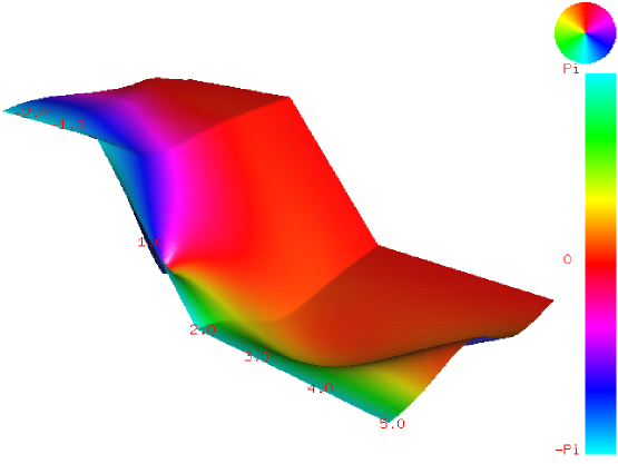
Figure 3: Configuration for $T/2=1.98$ and $\Theta=2.74$. $\varepsilon=0.711$. Height and color represent $|\chi|$ and the phase of $\chi$, respectively. For visualization purposes the Euclidean part of the contour is inclined.

A typical configuration is shown in figure 3. One can clearly see that the phase of the field $\chi$ behaves as shown in figure 2, going from $-\pi$ at $r=0$ to $\pi$ at $r=L$ along different sides of the circle in the initial and final states. In the middle of the Euclidean region, a zero of the field $\chi$ is present (center of the “instanton”). Also the incoming/outgoing wave is observed at initial/final Minkowskian part.

It is fairly straightforward to check that the singularities shown in figure (1) are indeed present, by continuing the solution from the part BC of the contour to the whole complex time plane. The left singularity is approximately at the same distance from the Euclidean part of the contour for all solutions. The right singularity moves to larger positive times as the energy increases.

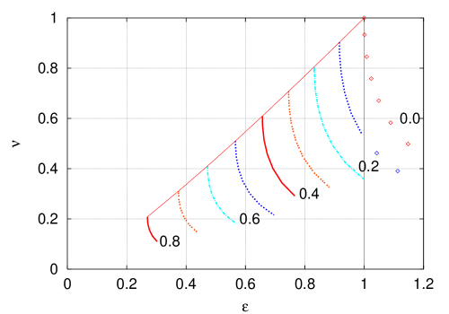
Figure 4: Lines of $F(\varepsilon,\nu)=\mathrm{const}$. $F$ is normalized to be unity at $\nu=\varepsilon=0$ (instanton). Diagonal line directed from sphaleron ($\nu=\varepsilon=1$) towards the origin is the line of periodic instantons. Open symbols correspond to configurations with wrong topology. Numbers near the curves show the suppression factor $F$.

Summary of the results is given in figure 4. Lines of constant suppression factor $F$ are shown on $\varepsilon$–$\nu$ plane. Units are normalized to the sphaleron: $\nu_{\mathrm{sph}}=\varepsilon_{\mathrm{sph}}=1$.

Behavior of the constant suppression lines has the following features. Near the periodic instanton ($\Theta=0$), the dependence of $F$ on $\nu$ is weak. This can be seen analytically from the boundary problem (3) itself. Making use of the fact that $F$ is stationary with respect to $T$ and $\Theta$ one finds

$$\left.\frac{dN}{dE}\right|_{F=\mathrm{const}}=-\frac{T}{\Theta}\;,$$

which is infinite as $\Theta\to 0$.

When one moves away from the periodic instantons, lines of constant $F$ flatten out; in other words, increase of energy in this region leads to smaller decrease of the suppression exponent than in the vicinity of the periodic instanton.

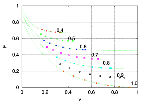
Figure 5: Dependence of the suppression factor $F$ on $\nu$ for different energies. Numbers near the curves show values of $\varepsilon$. Lines are extrapolations of data with functions of the form $ae^{-b\nu}-c$.

The quantity of primary interest is the two-particle cross section

$$\sigma_{\mathrm{tot}}(E)\sim\exp\left\{-\frac{16\pi^{2}}{g^{2}}F\left({E}/{E_{\mathrm{sph}}},0\right)\right\}$$

We can plot $F(\varepsilon,\nu)$ as a function of $\nu$ for different values of energy (fig. 5). Extrapolation of the data for $\varepsilon=0.4,\dots,1.0$ crosses the line $\nu=0$ at $F\sim 0.8,\dots,1$. So we conclude that for energies below the sphaleron, the exponent of the suppression factor of the tunneling processes is only about 20% less than for zero energy (instanton case).

Finally, the open symbols in fig. 4 correspond to evolutions where the field configuration, after having undergone a topological transition (marked by the zero of the $\chi$ field on BC part of the time contour—see fig. 3), goes trough a reverse transition on the CD part of the contour and returns to the original topological sector. We will discuss these solutions in the next section.

5 Conclusions and Outlook

Of course, the point of major interest is whether at sufficiently high energy particle collisions can induce unsuppressed topological transitions and baryon number violation in the Electroweak Theory. In terms of the graph of fig. 4 the question is whether the line corresponding to $F(\varepsilon,\nu)=0$ does approach the $\nu=0$ axis asymptotically for increasing $\varepsilon$ and, if it does, at what rate.

It should be noted that in our study we have not yet been able to obtain topology changing solutions with $F=0$. As we described, the exploration of the space of solutions is done through a deformation procedure, by which the parameters $T$ and $\Theta$ are gradually changed. This in turn moves the solutions in the $\varepsilon,\nu$ plane. We observed that as one goes beyond the sphaleron energy, the solutions become unstable. The field configurations linger for longer and longer times in the neighborhood of the sphaleron and then return to the original topological sector. One thus obtains solutions satisfying the equations of motion and all the boundary conditions, but for the requirement that the topology changes. This instability is not unexpected. It was observed by the authors of ref. [24] in their study of transitions across a potential barrier in a quantum mechanical model. It indicates a likely bifurcation in the space of semiclassical solutions as one reaches the barrier energy. In ref. [24] the problem was solved by deforming the time contour for the evolution (see fig. 1) to make it go below the real axis (the segment CD in fig. 1) before returning to the real time axis. This helped pinpoint a set of solutions with transition across the barrier. We are pursuing a similar strategy in our current search. The computational problems one faces are nevertheless daunting. The most crucial factor is the ability of following the solutions for negative and positive time well into the linear regime, where they are settled in the two different different topological sectors. This in turn requires the use of a grid of large extent in the radial direction and makes the computation quite demanding. We are making progress and hope that we will be able to report on topology changing solutions above the sphaleron energy in the near future. For the moment, we believe that the detailed information we obtained for the lines of constant suppression factor below the sphaleron energy can also be of value. In particular, the marked bending of the lines toward increasing energy as one lowers the incoming particle number seems to indicate that topology changing transitions in particle collisions will occur, if at all, only for energy substantially higher than $E_{\mathrm{sph}}$.

6 Acknowledgements

The authors are grateful to A.Kuznetsov for numerous discussions at different stages of the work.

This work has supported in part under DOE grant DE-FG02-91ER40676 and by Award RP1-2103 of the U.S. Civilian Research & Development Foundation (CRDF). F.B. and V.R. are supported also by Russian Foundation for Basic Research (RFBR) grant 99-01-18410; Council for Presidential Grants and State Support of Leading Scientific Schools, grant 00-15-96626. P.T. is supported by the Swiss Science Foundation, grant 21-58947.99.

References

- [1] G. ’t Hooft, Phys. Rev. D14 (1976) 3432,
- [2] S. Coleman, Phys. Rev. D15 (1977) 2929,
- [3] A.A. Belavin et al., Phys. Lett. B59 (1975) 85,
- [4] V.A. Kuzmin, V.A. Rubakov and M.E. Shaposhnikov, Phys. Lett. 155B (1985) 36,
- [5] P. Arnold and L. McLerran, Phys. Rev. D36 (1987) 581,
- [6] P. Arnold and L. McLerran, Phys. Rev. D37 (1988) 1020,
- [7] V.A. Rubakov and A.N. Tavkhelidze, Phys. Lett. B165 (1985) 109,
- [8] V.A. Matveev et al., Nucl. Phys. B282 (1987) 700,
- [9] D.V. Deryagin, D.Y. Grigoriev and V.A. Rubakov, Phys. Lett. B178 (1986) 385,
- [10] V.A. Rubakov, JETP Lett. 41 (1985) 266,
- [11] J. Ambjorn and V.A. Rubakov, Nucl. Phys. B256 (1985) 434,
- [12] V.A. Rubakov, B.E. Stern and P.G. Tinyakov, Phys. Lett. 160B (1985) 292,
- [13] A. Ringwald, Nucl. Phys. B330 (1990) 1,
- [14] O. Espinosa, Nucl. Phys. B343 (1990) 310,
- [15] L. McLerran, A. Vainshtein and M. Voloshin, Phys. Rev. D42 (1990) 171,
- [16] S.Y. Khlebnikov, V.A. Rubakov and P.G. Tinyakov, Nucl. Phys. B350 (1991) 441,
- [17] L.G. Yaffe, Talk given at Santa Fe Workshop on Baryon Violation at the SSC, Santa Fe, NM, Apr 27-30, 1990.
- [18] P.B. Arnold and M.P. Mattis, Mod. Phys. Lett. A6 (1991) 2059,
- [19] P.G. Tinyakov, Int. J. Mod. Phys. A8 (1993) 1823,
- [20] V.A. Rubakov and P.G. Tinyakov, Phys. Lett. B279 (1992) 165,
- [21] P.G. Tinyakov, Phys. Lett. B284 (1992) 410,
- [22] V.A. Rubakov, D.T. Son and P.G. Tinyakov, Phys. Lett. B287 (1992) 342,
- [23] A.H. Mueller, Nucl. Phys. B401 (1993) 93,
- [24] G.F. Bonini et al., Phys. Rev. D60 (1999) 076004, hep-ph/9901226,
- [25] A.N. Kuznetsov and P.G. Tinyakov, Phys. Rev. D56 (1997) 1156, hep-ph/9703256,
- [26] N.S. Manton, Phys. Rev. D28 (1983) 2019,
- [27] F.R. Klinkhamer and N.S. Manton, Phys. Rev. D30 (1984) 2212,
- [28] C. Rebbi and J. Robert Singleton, Phys. Rev. D54 (1996) 1020, hep-ph/9601260,
- [29] S.Y. Khlebnikov, V.A. Rubakov and P.G. Tinyakov, Nucl. Phys. B367 (1991) 334,
- [30] G.F. Bonini et al., (1999), hep-ph/9905243,
- [31] J.R. Espinosa and M. Quiros, Phys. Lett. B266 (1991) 389,
- [32] B. Ratra and L.G. Yaffe, Phys. Lett. B205 (1988) 57,