Spin Correlations in Monte Carlo Simulations

Abstract:

We show that the algorithm originally proposed by Collins and Knowles for spin correlations in the QCD parton shower can be used in order to include spin correlations between the production and decay of heavy particles in Monte Carlo event generators. This allows correlations to be included while maintaining the step-by-step approach of the Monte Carlo event generation process.

We present examples of this approach for both the Standard and Minimal Supersymmetric Standard Models. A merger of this algorithm and that used in the parton shower is discussed in order to include all correlations in the perturbative phase of event generation. Finally we present all the results needed to implement this algorithm for the Standard and Minimal Supersymmetric Standard Models.

1 Introduction

In modern particle physics experiments it is important to have a Monte Carlo simulation which accurately predicts the results of the experiment for both those processes which have already been observed and any new physics which may be discovered. As higher energies are probed this often means the production of heavy particles which decay before hadronizing giving decay products which are detected, e.g.  the top quark.

As these particles are often fermions the distributions of the decay products are affected by correlations between the production and decay of the fermion. In most Monte Carlo event generators these correlations are neglected. In the Standard Model (SM) this only applies to the top quark and tau lepton. However, in most models of new physics, for example supersymmetry, there are heavy fermions which decay and correlations between the production and decay of these fermions may be important [1, 2, 3, 4].

There have been a number of calculations of the spin correlation effects for specific processes, but these calculations all require the hard collision process and the decay of the heavy fermions to be performed in the same step which is problematic in Monte Carlo event generators.

There are however methods [5, 6, 7, 8] which have previously been used in order to correlate all the partons produced in the QCD parton shower. In this paper we shall show how a very similar algorithm can be used in order to correlate the spins of all the heavy particle decays in the event while still maintaining both the step-by-step approach of the Monte Carlo event generator and an algorithm whose complexity grows only linearly with the number of particles.

In the next section we will review the ideas of Monte Carlo simulations and discuss the current implementation of heavy particle decays in event generators. This is followed by a discussion of the algorithm we will use in Section 3. We provide several examples of the results of this algorithm for both Standard Model and supersymmetric (SUSY) processes in Section 4. We then discuss how to incorporate spin correlations in the decay of heavy particles as well as the spin correlations inside and between jets which are already included in some Monte Carlo event generators [9, 10] using the algorithm of [5, 6, 7, 8]. Finally, we present the necessary results in order to implement this algorithm for both Standard and Minimal Supersymmetric Standard Model processes.

2 Monte Carlo Event Generation

There are a number of general purpose Monte Carlo event generators available [11, 12, 13, 9, 10]. The structure of the event generation procedure is basically the same in all these programs. The differences are in the algorithms used in the different steps of generating the event. In general the Monte Carlo event generation process can be divided into five phases:

1. The hard process where the particles in the hard collision and their momenta are generated, usually according to the leading-order matrix element. This can be of either the incoming fundamental particles in lepton collisions or of a parton extracted from a hadron in hadron-initiated processes. In the example event shown in Fig. 1 the hard process is $\mathrm{e^{+}e^{-}\rightarrow t\bar{t}}$.

2. The parton-shower phase where the coloured particles in the event are perturbatively evolved from the hard scale of the collision to the infrared cut-off. This is done for both the particles produced in the collision, the final-state shower, and the initial partons involved in the collision for processes with incoming hadrons, the initial-state shower. In the example shown in Fig. 1 the top quarks radiate gluons and the gluons branch.

3. Those particles which decay before hadronizing, e.g.  the top quark and SUSY particles, are then decayed. Any coloured particles produced in these secondary decays are evolved by the parton-shower algorithm. These decays are usually performed according to a calculated branching ratio and often use a matrix element to give the momenta of the decay products. The example in Fig. 1 shows the semi-leptonic decay of both top quarks.

4. A hadronization phase in which the partons left after the perturbative evolution are formed into the observed hadrons. For processes with hadrons in the initial state after the removal of the partons in the hard process, we are left with a hadron remnant. This remnant is also formed into hadrons by the hadronization model. In the example shown in Fig. 1 the cluster model [14], which is used in HERWIG [9, 10], is shown.

5. Those unstable hadrons which are produced in the hadronization phase must also be decayed. These decays are usually performed using the experimentally measured branching ratios and a phase-space distribution for the momenta of the decay products. Any coloured particles produced in these decays are evolved according to the parton-shower algorithm and hadronized. This procedure is repeated until all the unstable particles have been decayed.

Figure 1: Example of a Monte Carlo event. This example shows the production of $\mathrm{t\bar{t}}$ in $\mathrm{e}^{+}\mathrm{e}^{-}$ collisions followed by the semi-leptonic decay of the top quarks. The cluster hadronization model [14] is shown where the gluons left after the parton-shower phase are non-perturbatively split into quark-antiquark pairs. The quarks and antiquarks are then paired into colour-singlet clusters using the colour flow information in the event. These clusters decay to give the observed hadrons.

In the Standard Model the only quark which decays before hadronizing is the top quark. It is therefore possible to include $\mathrm{t\bar{t}}$ production, including spin effects, as a $2\to 6$ process, i.e. including the decay of the top quarks, in a Monte Carlo event generator. However this leads to problems when including QCD radiation from the top quark before it decays.

In all Monte Carlo event generators the particles are produced and then QCD radiation is generated via the parton-shower algorithm. Any unstable particles are then decayed. This is the main problem for the inclusion of spin correlations, i.e. we want to be able generate the production and decay of the particles as separate processes rather than in one step so that QCD radiation can be generated for the particles before they decay.

The problem is somewhat different for the inclusion of tau decays due to the large number of tau decay modes. This makes it impossible to include all the possible decay channels as $2\to n$ body processes.

The situation in SUSY models is similar to that for tau decays. In order to facilitate the experimental search for supersymmetry a number of Monte Carlo event generators have either been extended to include supersymmetric processes [15, 11, 12, 13, 16, 9, 10], or written specifically for the study of supersymmetry [17, 18].

These event generators have become increasingly sophisticated in their treatment of supersymmetric processes. In general, the decays of the supersymmetric particles produced in the hard collision process are assumed to take place independently. The event generators differ in how these decays are performed. While HERWIG [16, 9, 10] continues to use a phase-space distribution for the three-body decays of the supersymmetric particles ISAJET [13], PYTHIA [15, 11, 12] and SUSYGEN [17, 18] use the full three-body matrix element.

A number of studies have also been performed in which spin correlation effects are included, and these have been shown to be important for a future linear collider [1, 2, 3, 4]. Some spin correlation effects have been included in SUSYGEN[17, 18]. However in order to accomplished this both the production process and decays must be generated at the same time which limits both the number of processes and final-state particles that can be simulated in this way.

In general SUSY models, particularly in hadron collisions, very complicated decay chains can occur and it is impossible to generate them all as $2\to n$ particle processes. We therefore need an algorithm which both preserves the step-by-step approach of the traditional Monte Carlo event generators and a complexity which does not grow exponentially with the number of final-state particles.

In this paper we will show that a completely general algorithm can be implemented which takes all these effects into account while still maintaining the step-by-step approach of the Monte Carlo event generation process. The results from the implementation of this algorithm in the HERWIG event generator are then compared to matrix element calculations from a number of observables.

3 Spin Correlation Algorithm

The spin correlation algorithm we will use is essentially identical to that presented in [5, 6, 7, 8] for the case of spin correlations in the QCD parton-shower phase of the Monte Carlo event generation process. However, the algorithm presented in [5, 6, 7, 8] only considers the case of $1\to 2$ branchings, as these are all that occur in the QCD parton shower.

The algorithm can be formulated entirely in terms of the matrix elements for the hard process and the various decays, spin density and decay matrices. The algorithm is defined as follows:

1. The momenta of the particles in the hard process are generated according to the matrix element

   $$\rho^{1}_{\kappa_{1}\kappa^{\prime}_{1}}\rho^{2}_{\kappa_{2}\kappa^{\prime}_{2}}\mathcal{M}_{\kappa_{1}\kappa_{2};\lambda_{1}\ldots\lambda_{n}}\mathcal{M}^{*}_{\kappa^{\prime}_{1}\kappa^{\prime}_{2};\lambda^{\prime}_{1}\ldots\lambda^{\prime}_{n}}\prod_{i=1,n}D^{i}_{\lambda_{i}\lambda^{\prime}_{i}},$$ (1)

   where $\mathcal{M}_{\kappa_{1},\kappa_{2};\lambda_{1}\ldots\lambda_{n}}$ is the matrix element for the $2\to n$ body process, $\kappa_{i}$ is the helicity of the $i$th incoming particle, $\lambda_{i}$ is the helicity of the $i$th outgoing particle, $\rho^{i}_{\kappa_{i}\kappa^{\prime}_{i}}$ is the spin density matrix for the $i$th incoming particle and $D^{i}_{\lambda_{i}\lambda^{\prime}_{i}}$ is the decay matrix for the $i$th outgoing particle.

   In the initial stage of the algorithm the momenta of the particles involved in the hard collision are generated according to Eqn. 1 with $D^{i}_{\lambda_{i}\lambda^{\prime}_{i}}=\delta_{\lambda_{i}\lambda^{\prime}_{i}}$ and $\rho^{i}_{\kappa_{i}\kappa^{\prime}_{i}}=\frac{1}{2}\delta_{\kappa_{i}\kappa^{\prime}_{i}}$ for unpolarized incoming particles. For polarized incoming particles

   $$\rho_{\kappa\kappa^{\prime}}=\left(\begin{array}[]{cc}\frac{1}{2}(1+\mathcal{P}_{3})&0\\ 0&\frac{1}{2}(1-\mathcal{P}_{3})\end{array}\right),$$ (2)

   where $\mathcal{P}_{3}$ is the component of the polarization vector parallel to the beam direction. For incoming antiparticles the sign of $\mathcal{P}_{3}$ must be changed.

2. One of the outgoing particles is chosen at random and a spin density matrix

   $$\rho_{\lambda_{j}\lambda^{\prime}_{j}}=\frac{1}{N_{\rho}}\rho^{1}_{\kappa_{1}\kappa^{\prime}_{1}}\rho^{2}_{\kappa_{2}\kappa^{\prime}_{2}}\mathcal{M}_{\kappa_{1}\kappa_{2};\lambda_{1}\ldots\lambda_{j}\ldots\lambda_{n}}\mathcal{M}^{*}_{\kappa^{\prime}_{1}\kappa^{\prime}_{2};\lambda^{\prime}_{1}\ldots\lambda^{\prime}_{j}\ldots\lambda^{\prime}_{n}}\prod_{i\neq j}D^{i}_{\lambda_{i}\lambda^{\prime}_{i}},$$ (3)

   calculated for the decay of this particle. The normalization

   $$N_{\rho}=\rho^{1}_{\kappa_{1}\kappa^{\prime}_{1}}\rho^{2}_{\kappa_{2}\kappa^{\prime}_{2}}\mathcal{M}_{\kappa_{1}\kappa_{2};\lambda_{1}\ldots\lambda_{j}\ldots\lambda_{n}}\mathcal{M}^{*}_{\kappa^{\prime}_{1}\kappa^{\prime}_{2};\lambda^{\prime}_{1}\ldots\lambda_{j}\ldots\lambda^{\prime}_{n}}\prod_{i\neq j}D^{i}_{\lambda_{i}\lambda^{\prime}_{i}},$$ (4)

   is chosen so that the trace of the spin density matrix is one.

3. The decay mode of this particle is selected according to the branching ratios and the momenta of the particles produced in the $n$-body decay generated according to

   $$\rho_{\lambda_{0}\lambda^{\prime}_{0}}\mathcal{M}_{\lambda_{0};\lambda_{1}\ldots\lambda_{n}}\mathcal{M}^{*}_{\lambda^{\prime}_{0};\lambda^{\prime}_{1}\ldots\lambda^{\prime}_{n}}\prod_{i=1,n}D^{i}_{\lambda_{i}\lambda^{\prime}_{i}},$$ (5)

   where $\lambda_{0}$ is the helicity of the decaying particle and $\lambda_{i}$ is the helicity of the $i$th decay product. As before the decay matrices are taken to be $D^{i}_{\lambda_{i}\lambda^{\prime}_{i}}=\delta_{\lambda_{i}\lambda^{\prime}_{i}}$ for the initial step of the algorithm.

4. One of the particles produced in this decay is selected and a spin density matrix

   $$\rho_{\lambda_{j}\lambda^{\prime}_{j}}=\frac{1}{N_{D\rho}}\rho_{\lambda_{0}\lambda^{\prime}_{0}}\mathcal{M}_{\lambda_{0};\lambda_{1}\ldots\lambda_{j}\ldots\lambda_{n}}\mathcal{M}^{*}_{\lambda^{\prime}_{0};\lambda^{\prime}_{1}\ldots\lambda^{\prime}_{j}\ldots\lambda^{\prime}_{n}}\prod_{i\neq j}D^{i}_{\lambda_{i}\lambda^{\prime}_{i}}$$ (6)

   calculated. Again the normalization

   $$N_{D\rho}=\rho_{\lambda_{0}\lambda^{\prime}_{0}}\mathcal{M}_{\lambda_{0};\lambda_{1}\ldots\lambda_{j}\ldots\lambda_{n}}\mathcal{M}^{*}_{\lambda^{\prime}_{0};\lambda^{\prime}_{1}\ldots\lambda_{j}\ldots\lambda^{\prime}_{n}}\prod_{i\neq j}D^{i}_{\lambda_{i}\lambda^{\prime}_{i}},$$ (7)

   is chosen such that the spin density matrix has unit trace. This spin density matrix is used as the input to the third step of the algorithm.

5. The third and fourth steps are repeated until the particle selected in step four is stable. When this occurs the decay matrix for this stable particle is set to $D^{i}_{\lambda_{i}\lambda^{\prime}_{i}}=\delta_{\lambda_{i}\lambda^{\prime}_{i}}$ and another particle from that decay selected to be decayed next using a spin density matrix for this particle calculated using Eqn. 6. When all the particles produced in a given decay have been developed a decay matrix

   $$D_{\lambda_{0}\lambda^{\prime}_{0}}=\frac{1}{N_{D}}\mathcal{M}_{\lambda_{0};\lambda_{1}\ldots\lambda_{n}}\mathcal{M}^{*}_{\lambda^{\prime}_{0};\lambda^{\prime}_{1}\ldots\lambda^{\prime}_{n}}\prod_{i=1,n}D^{i}_{\lambda_{i}\lambda^{\prime}_{i}},$$ (8)

   is calculated for the decay. Again the normalization

   $$N_{D}=\mathcal{M}_{\lambda_{0};\lambda_{1}\ldots\lambda_{n}}\mathcal{M}^{*}_{\lambda_{0};\lambda^{\prime}_{1}\ldots\lambda^{\prime}_{n}}\prod_{i=1,n}D^{i}_{\lambda_{i}\lambda^{\prime}_{i}},$$ (9)

   is chosen such that the trace of the decay matrix is one.

6. A new particle is selected from the decay which produced the decaying particle. This new particle has a spin density matrix given by Eqn. 6 using the decay matrix calculated from Eqn. 8 for the particles which have already been decayed rather than the identity. In this way the decay products of this particle will have the correct correlations with the decay products of the other particles produced in the same decay. This step is repeated until all the particles produced in a decay are developed. Eqn. 8 is then used to compute the decay matrix for this decay and the previous decay in the chain is developed.

7. Eventually this will give a decay matrix for the particle produced in the hard process. At this point a new particle from the hard process is selected to be decayed with a spin density matrix given by Eqn. 3 with the identity replaced by the calculated decay matrix for those particles which have already been decayed. In this way the correlations between the decays of the particles produced in the hard process are generated. This is repeated until all the particles produced in the hard process have been decayed.

At each point in the algorithm the normalization is chosen such that the trace of the spin density and decay matrices is one. This is necessary in order to maintain the probabilistic interpretation of the spin density matrices and proves to be usefully for the decay matrices.

4 Examples

There are many quantities for which it is interesting to calculate the spin correlations. In this section we will merely show a few examples of the method we propose for including the spin correlations and comparisons with the full analytic result for these quantities. Due to the complexities in calculating these full results this will limit us to relatively simple observables, although in principle much more complicated quantities can be calculated. The quantities have been chosen to both illustrate the technique and be phenomenogically important.

4.1 ${\mathrm{\tilde{q}}}_{L}\rightarrow{\rm q}\tilde{\chi}^{0}_{2}\rightarrow{\rm q}\ell^{\pm}\tilde{\ell}_{R}^{\mp}$

In hadron-hadron collisions the coloured SUSY particles, i.e. the squarks and gluinos, are preferentially produced and therefore the main source of electroweak gaugino and slepton production can be in the cascade decays of the coloured sparticles.

In many models the decay chain ${\mathrm{\tilde{q}}}_{L}\rightarrow{\rm q}\tilde{\chi}^{0}_{2}\rightarrow{\rm q}\ell^{\pm}\tilde{\ell}_{R}^{\mp}\rightarrow{\rm q}\ell^{+}\ell^{-}\tilde{\chi}^{0}_{1}$, Fig. 2, is important because by studying edges in the $\ell^{+}\ell^{-}$, ${\rm q}\ell^{\pm}$ and ${\rm q}\ell^{+}\ell^{-}$ mass distributions the masses of the lightest two neutralinos, squark and slepton can be reconstructed [19, 20, 22, 21, 23].

Figure 2: Feynman Diagrams for the decay ${\rm\tilde{q}}_{L}\rightarrow{\rm q}\tilde{\chi}^{0}_{2}\rightarrow{\rm q}\ell^{\pm}\tilde{\ell}^{\mp}_{R}$.

However, if we consider the spins of the particles involved the quark produced in the squark decay will be left-handed in the massless limit. The lepton produced in the neutralino decay will be right-handed. This will lead to very different decay distributions for the charge conjugate decay modes of the neutralino.

This difference is most noticeable in distribution of the mass of the quark and the lepton produced in the neutralino decay, Fig. 3. The results in Fig. 3 were generated at SUGRA point 5 [20, 24], i.e. $M_{0}=200\,\rm{\,GeV}$, $M_{1/2}=300\,\rm{\,GeV}$, $A_{0}=300\,\rm{\,GeV}$, $\tan\beta=2.1$ and $\mathrm{sgn}\,\mu+$, where $M_{0}$ is the universal SUSY breaking scalar mass at the Grand Unified Theory (GUT) scale, $M_{1/2}$ is the universal SUSY breaking gaugino mass at the GUT scale, $A_{0}$ is the universal tri-linear soft SUSY breaking parameter at the GUT scale, $\mathrm{sgn}\,\mu$ is the sign of the $\mu$ parameter and $\tan\beta$ is the ratio of the two Higgs vacuum expectation values. At this SUGRA point the squark mass $M_{{\rm\tilde{q}}_{L}}=833.8\,\rm{\,GeV}$, the lightest neutralino mass $M_{\tilde{\chi}^{0}_{1}}=115.5\,\rm{\,GeV}$ and the next-to-lightest neutralino mass $M_{\tilde{\chi}^{0}_{2}}=213.2\,\rm{\,GeV}$. The SUSY spectrum was generated using ISAJET7.51 [13].

The differences in the shapes of the two distributions in Fig. 3 can be understood by considering the helicities of the particles, the quark is left-handed while the produced lepton/antilepton is right-handed. In the case of an antilepton this means that if the antilepton and the quark are back-to-back they have no net spin and therefore this configuration which gives the edge in the mass distribution shown in Fig. 3a is favoured. However, if a lepton is produced this configuration has net spin one and therefore cannot be produced in the decay of a scalar so the distribution in Fig. 3b vanishes at the end point.

Unfortunately in any experiment there is no way to distinguish between a quark and an antiquark. Hence the average of the distributions in Fig. 3 will be observed. This average is in good agreement with the phase-space distribution.

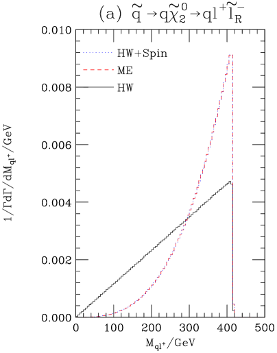
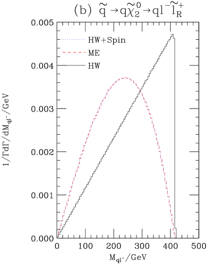
Figure 3: Distribution of the mass of quark and lepton produced in the decay ${\rm\tilde{q}}_{L}\rightarrow{\rm q}\tilde{\chi}^{0}_{2}\rightarrow{\rm q}\ell^{\pm}\tilde{\ell}^{\mp}_{R}$. The solid line gives the result of phase space, the dashed line gives the full result and the dotted line the result of the spin correlation algorithm.

This is the simplest, non-trivial, application of the spin correlation algorithm. Here all that is necessary is that the spin density matrix for the production of the neutralino in the scalar decay is used to perform the decay of the neutralino to a scalar and a fermion. The matrix elements are therefore relatively simple. Indeed the matrix elements are simple enough to allow us to compare the results of the algorithm and the full result analytically. The matrix element for the 3-body process ${\rm\tilde{q}}_{L}\rightarrow{\rm q}\tilde{\chi}^{0}_{2}\rightarrow{\rm q}\ell^{+}\tilde{\ell}_{R}^{-}$ is given by

$$\mathcal{M}_{{\rm\tilde{q}}_{L}\rightarrow{\rm q}\tilde{\chi}^{0}_{2}\rightarrow{\rm q}\ell^{+}\tilde{\ell}_{R}^{-}} = \bar{u}(p_{{\rm q}})a^{\lambda}P_{\lambda}\left(p\!\!\!\!\!\not\>\>\!_{\chi}-M_{\chi}\right)b^{\lambda^{\prime}}P_{\lambda^{\prime}}v(p_{\ell}),$$ (10)

where $p_{\tilde{\chi}}$ is the four-momentum of the neutralino, $p_{{\rm q}}$ is the four-momentum of the quark, $p_{\ell}$ is the four-momentum of the produced lepton, $P_{\lambda}=\frac{1}{2}(1+\lambda\gamma_{5})$ , $a^{\lambda}$ and $b^{\lambda}$ are the couplings for the production and decay of the neutralino, respectively. In the notation used in Appendix B, $a^{\lambda}=a^{*-\lambda}_{\tilde{\chi}^{0}_{2}{\rm\tilde{q}}_{i1}{\rm q}_{i}}$ and $b^{\lambda}=a^{\lambda}_{\tilde{\chi}^{0}_{2}\tilde{\ell}_{i2}\ell_{i}}$ where in the limit that we neglect left/right sfermion mixing $Q^{i}_{\alpha\beta}=\delta_{\alpha,\beta=1}$ for left squarks and $L^{i}_{\alpha\beta}=\delta_{\alpha,\beta=2}$ for right sleptons. As the width of the neutralino is small compared to its mass we have assumed that it is on-mass-shell.

We can now consider how the spin correlation algorithm attempts to reproduce this result. The matrix element for the first step of the process is

$$\mathcal{M}_{{\rm\tilde{q}}_{L}\rightarrow{\rm q}\tilde{\chi}^{0}_{2}} = \bar{u}(p_{{\rm q}})a^{\lambda}P_{\lambda}v(p_{\tilde{\chi}}),$$ (11a)

$$= -\frac{1}{2\sqrt{p_{\tilde{\chi}}\cdot l_{\tilde{\chi}}p_{{\rm q}}\cdot l_{{\rm q}}}}\bar{u}_{-\lambda_{{\rm q}}}(l_{{\rm q}})\left(p\!\!\!\!\!\not\>\>\!_{{\rm q}}a^{\lambda_{{\rm q}}}+m_{{\rm q}}a^{-\lambda_{{\rm q}}}\right)(p_{\tilde{\chi}}-m_{\tilde{\chi}})u_{\lambda_{\tilde{\chi}}}(l_{\tilde{\chi}}),\ \ \$$ (11b)

where $\lambda_{\tilde{\chi}}$ is the helicity of the neutralino, $\lambda_{{\rm q}}$ is the helicity of the quark, $l_{{\rm q}}$ and $l_{\tilde{\chi}}$ are the reference vectors for the quark and neutralino, respectively. The use of these reference vectors in defining the spinors for massive fermions is described in Appendix A. The sign of the helicity of the neutralino has be chosen in order for the outgoing neutralino to be considered as a particle rather than an antiparticle.

In the first stage of the algorithm the momenta of the neutralino and quark are generated according to the spin averaged matrix element

$$\sum_{\rm{spins}}|\mathcal{M}_{{\rm\tilde{q}}_{L}\rightarrow{\rm q}\tilde{\chi}^{0}_{2}}|^{2}=2\left[p_{{\rm q}}\cdot p_{\tilde{\chi}}\left({a^{+}}^{2}+{a^{-}}^{2}\right)-2a^{+}a^{-}m_{{\rm q}}m_{\tilde{\chi}}\right].$$ (12)

As the quark is stable we can average over its spin and produce the spin density matrix needed to perform the decay of the neutralino,

$$\rho_{\lambda_{\tilde{\chi}}\lambda^{\prime}_{\tilde{\chi}}} = \frac{1}{N}\frac{1}{2p_{\tilde{\chi}}\cdot l_{\tilde{\chi}}}\bar{u}_{\lambda^{\prime}_{\tilde{\chi}}}(l_{\tilde{\chi}})(p\!\!\!\!\!\not\>\>\!_{\tilde{\chi}}-m_{\tilde{\chi}})$$

$$\left[\left(p\!\!\!\!\!\not\>\>\!_{{\rm q}}{a^{-}}^{2}+m_{{\rm q}}a^{+}a^{-}\right)P_{+}+\left(p\!\!\!\!\!\not\>\>\!_{{\rm q}}{a^{+}}^{2}+m_{{\rm q}}a^{+}a^{-}\right)P_{-}\right](p\!\!\!\!\!\not\>\>\!_{\tilde{\chi}}-m_{\tilde{\chi}})u_{\lambda_{\tilde{\chi}}}(l_{\tilde{\chi}}),$$

where the normalization $N$ is chosen to give $\sum_{\lambda}\rho_{\lambda\lambda}=1$ and is therefore equal to the spin averaged matrix element, Eqn. 12.

The matrix element for the decay of the neutralino is given by

$$\mathcal{M}^{\lambda_{\tilde{\chi}}}_{\tilde{\chi}^{0}_{2}\rightarrow\ell^{+}\tilde{\ell}_{R}^{-}} = \bar{u}(p_{\tilde{\chi}})b^{\lambda}P_{\lambda}v(p_{\ell}),$$ (14a)

$$= -\frac{1}{2\sqrt{p_{\tilde{\chi}}\cdot l_{\tilde{\chi}}p_{\ell}\cdot l_{\ell}}}\bar{u}_{\lambda_{\tilde{\chi}}}(l_{\tilde{\chi}})\left(p\!\!\!\!\!\not\>\>\!_{\tilde{\chi}}-m_{\tilde{\chi}}\right)\left[p\!\!\!\!\!\not\>\>\!_{\ell}b^{\lambda_{\ell}}-m_{\ell}b^{-\lambda_{\ell}}\right]u_{\lambda_{\ell}}(l_{\ell}),\ \ \ \$$ (14b)

where $p_{\ell}$ is the four-momentum of the lepton, $l_{\ell}$ is the reference vector used to define the direction of the lepton’s spin and $\lambda_{\ell}$ is the helicity of the lepton.

As with the quark because the produced lepton is stable we can average over its helicities giving

$$\mathcal{M}_{\tilde{\chi}^{0}_{2}\rightarrow\ell^{+}\tilde{\ell}_{R}^{-}}^{\lambda_{\tilde{\chi}}}\mathcal{M}_{\tilde{\chi}^{0}_{2}\rightarrow\ell^{+}\tilde{\ell}_{R}^{-}}^{\lambda^{\prime}_{\tilde{\chi}}*} = \frac{1}{2p_{\tilde{\chi}}\cdot l_{\tilde{\chi}}}\bar{u}_{\lambda_{\tilde{\chi}}}(l_{\tilde{\chi}})\left(p\!\!\!\!\!\not\>\>\!_{\tilde{\chi}}-m_{\tilde{\chi}}\right)$$

$$\left[\left(p\!\!\!\!\!\not\>\>\!_{\ell}{b^{+}}^{2}-m_{\ell}b^{+}b^{-}\right)P_{-}+\left(p\!\!\!\!\!\not\>\>\!_{\ell}{b^{-}}^{2}-m_{\ell}b^{+}b^{-}\right)P_{+}\right]$$

$$\left(p\!\!\!\!\!\not\>\>\!_{\tilde{\chi}}-m_{\tilde{\chi}}\right)u_{\lambda^{\prime}_{\tilde{\chi}}}(l_{\tilde{\chi}}).$$

This can now be contracted with the spin density matrix and the sum over the helicities of the neutralino performed giving

$$\rho_{\lambda_{\tilde{\chi}}\lambda^{\prime}_{\tilde{\chi}}}\hbox to0.0pt{$\displaystyle\mathcal{M}_{\tilde{\chi}^{0}_{2}\rightarrow\ell^{+}\tilde{\ell}_{R}^{-}}^{\lambda_{\tilde{\chi}}}\mathcal{M}_{\tilde{\chi}^{0}_{2}\rightarrow\ell^{+}\tilde{\ell}_{R}^{-}}^{\lambda^{\prime}_{\tilde{\chi}}*}=$\hss}$$

$$\frac{1}{N}{\rm Tr}\,\left\{\left(p\!\!\!\!\!\not\>\>\!_{\tilde{\chi}}-m_{\tilde{\chi}}\right)\left[\left(p\!\!\!\!\!\not\>\>\!_{{\rm q}}{a^{-}}^{2}+m_{{\rm q}}a^{+}a^{-}\right)P_{+}+\left(p\!\!\!\!\!\not\>\>\!_{{\rm q}}{a^{+}}^{2}+m_{{\rm q}}a^{+}a^{-}\right)P_{-}\right]\right.$$

$$\ \ \ \ \ \ \,\ \left.\left(p\!\!\!\!\!\not\>\>\!_{\tilde{\chi}}-m_{\tilde{\chi}}\right)\left[\left(p\!\!\!\!\!\not\>\>\!_{\ell}{b^{+}}^{2}-m_{\ell}b^{+}b^{-}\right)P_{-}+\left(p\!\!\!\!\!\not\>\>\!_{\ell}{b^{-}}^{2}-m_{\ell}b^{+}b^{-}\right)P_{+}\right]\right\}.$$

The second decay is generated according to this formula. The normalization of the spin density matrix is cancelled by the matrix element which is used to generate the first decay. If we compare the above result with the matrix element for the full 3-body process we can see that it agrees with the amplitude squared. Hence, the decay products will have the same distribution as the full three-body matrix element. This can be seen in Fig. 3 where the result of the full 3-body matrix element and the spin correlation algorithm are in very good agreement.

4.2 $\rm{e^{+}e^{-}}\rightarrow\tilde{\chi}^{0}_{2}\tilde{\chi}^{0}_{1}$

Figure 4: Feynman diagrams for the production of $\tilde{\chi}^{0}_{2}\tilde{\chi}^{0}_{1}$ in $\rm{e}^{+}\rm{e}^{-}$ collisions.

In the MSSM the lightest supersymmetric particle (LSP), usually taken to be the lightest neutralino, is stable and weakly interacting. It therefore escapes from the detector without interacting giving missing transverse energy. This means that in a future linear collider the production of $\tilde{\chi}^{0}_{2}\tilde{\chi}^{0}_{1}$, Fig. 4, may well be the detectable supersymmetric final state which requires the smallest centre-of-mass energy. The production of the second-to-lightest-neutralino will be followed by its decay to the lightest neutralino. This decay will be $\tilde{\chi}^{0}_{2}\rightarrow\tilde{\chi}^{0}_{1}\rm{f}\rm{\bar{f}}$ via either real or virtual sfermions, Higgs or Z bosons, Fig. 5.

There have been a number of studies of spin correlations for this process both with [3, 4] and without [1] beam polarization. The study of both the decay correlations and polarization effects is important because it would allow the nature of the neutralinos to be determined.

This is a more complicated example of the use of the spin correlation algorithm than the squark decay we studied in the previous section. Instead of being produced in a scalar decay the neutralino is produced in a $2\to 2$ process where there are a number of Feynman diagrams and the possibility of polarizing the incoming particles. However, as before the spin correlation algorithm only has to compute the spin density matrix for the production and use this to generate the decay of the neutralino which may be via either a two or three body process, Fig. 5.

The easiest case to consider first is the decay of the neutralino to a lepton and a right-handed slepton, as in Section 4.1, again using SUGRA Point 5. As can be seen in Fig. 6 there is a correlation between the direction of the produced lepton and the beam direction and this correlation is affected by the polarization of the beam. It should be noted that fully polarized beams are not achievable in practice and are only shown in order to illustrate the results of the algorithm. As with the results in Section 4.1 the result of the spin correlation algorithm is in good agreement with the result from a 4-body matrix element including the decay of both the neutralino and slepton.

Figure 5: Feynman diagrams for the decay $\tilde{\chi}^{0}_{2}\rightarrow\rm{f}\bar{\rm{f}}\tilde{\chi}^{0}_{1}$. The exchange of the MSSM Higgs bosons is only important for the third generation of fermions.

It is also possible that neither the gauge boson or sleptons in the diagrams in Fig. 5 can be real. As an example we considered a SUGRA point with non-universal gaugino masses at the GUT scale in order to decrease the mass difference between the lightest two neutralinos. We used the point $M_{0}=210\,\rm{\,GeV}$, $A_{0}=0\,\rm{\,GeV}$, $\tan\beta=10$, $M_{1}=450\,\rm{\,GeV}$, $M_{2}=350\,\rm{\,GeV}$, $M_{3}=350\,\rm{\,GeV}$, where $M_{1}$ is the soft SUSY breaking mass for the bino at the GUT scale, $M_{2}$ is the soft SUSY breaking mass for the wino at the GUT scale and $M_{3}$ is the soft SUSY breaking mass for the gluino at the GUT scale. At this point the lightest neutralino is dominantly bino-like and the next-to-lightest neutralino is dominantly wino-like, the lightest neutralino mass is $M_{\tilde{\chi}^{0}_{1}}=182.4\,\rm{\,GeV}$, the next-to-lightest neutralino mass is $M_{\tilde{\chi}^{0}_{2}}=264.2\,\rm{\,GeV}$, the right-slepton mass is $M_{\tilde{\ell}_{R}}=271.3\,\rm{\,GeV}$ and the left-slepton mass is $M_{\tilde{\ell}_{L}}=322.5\,\rm{\,GeV}$. This point was chosen so that both the right-handed slepton and the Z boson could be almost on mass-shell in the three body decay $\tilde{\chi}^{0}_{2}\rightarrow\tilde{\chi}^{0}_{1}\ell^{+}\ell^{-}$.

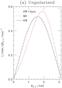
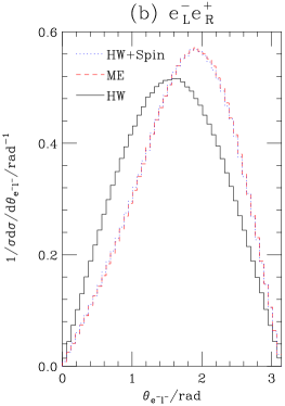
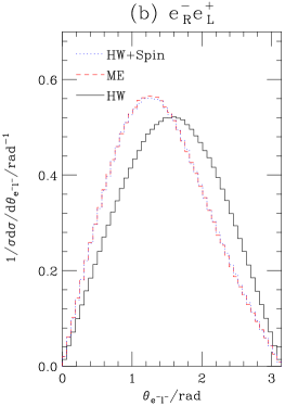
Figure 6: Angle between the lepton produced in $\rm{e}^{+}\rm{e}^{-}\rightarrow\tilde{\chi}^{0}_{2}\tilde{\chi}^{0}_{1}\rightarrow\tilde{\ell}^{+}_{R}\ell^{-}\tilde{\chi}^{0}_{1}$ and the incoming electron beam in the laboratory frame for a centre-of-mass energy of 500 GeV with (a) no polarization, (b) negatively polarized electrons and positively polarized positrons and (c) positively polarized electrons and negatively polarized positrons. The solid line shows the default result from HERWIG which treats the production and decay as independent, the dashed line gives the full result from the 4-body matrix element and the dotted line the result of the spin correlation algorithm.

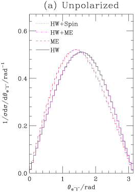
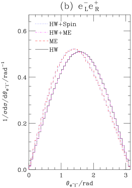
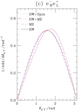
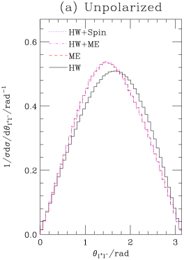
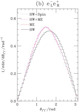
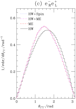
Figure 7: Angle between the lepton produced in $\rm{e}^{+}\rm{e}^{-}\rightarrow\tilde{\chi}^{0}_{2}\tilde{\chi}^{0}_{1}\rightarrow\ell^{+}\ell^{-}\tilde{\chi}^{0}_{1}\tilde{\chi}^{0}_{1}$ and the incoming electron beam in the laboratory frame for a centre-of-mass energy of 500 GeV with (a) no polarization, (b) negatively polarized electrons and positively polarized positrons and (c) positively polarized electrons and negatively polarized positrons. The solid line shows the default result from HERWIG which treats the production and decay as independent and uses a phase-space distribution for the decay products of the neutralino, the dot-dashed line also includes a matrix element for the neutralino decay, the dashed line gives the full result from the 4-body matrix element and the dotted line the result of the spin correlation algorithm.

Figure 8: Angle between the lepton and antilepton produced in $\rm{e}^{+}\rm{e}^{-}\rightarrow\tilde{\chi}^{0}_{2}\tilde{\chi}^{0}_{1}\rightarrow\ell^{+}\ell^{-}\tilde{\chi}^{0}_{1}\tilde{\chi}^{0}_{1}$ in the laboratory frame for a centre-of-mass energy of 500 GeV with (a) no polarization, (b) negatively polarized electrons and positively polarized positrons and (c) positively polarized electrons and negatively polarized positrons. The lines are described in the caption of Fig. 8.

The angle between the lepton produced in the $\tilde{\chi}^{0}_{2}$ decay and the beam is shown in Fig. 8 for a three choices of polarization for the incoming beams. The angle between the produced leptons is shown in Fig. 8 for the same choices of beam polarization. The default treatment of this process in the HERWIG event generator is that the production and decay of the next-to-lightest neutralino take place independently and the neutralino is decayed using a phase-space distribution for the decay products. We have therefore shown the result of using a matrix element to perform this decay, while still treating the production and decay as independent, as well as the result of the spin correlation algorithm and a full calculation of the process in Figs. 8 and 8.

As can be seen in Fig. 8 the inclusion of the matrix element for the decay on its own has no effect on the angle between the lepton and the beam, whereas the inclusion of this matrix element significantly improves the agreement between the result of HERWIG and the full result for the distribution of the angles between the produced lepton and antilepton, Fig. 8. Indeed the inclusion of the matrix element seems to be all that is required in order for the Monte Carlo simulation to reproduce the full result for this distribution. The full spin correlation algorithm is necessary to reproduce the correlation between the beam direction and the direction of the produced lepton. Again, there is good agreement between the full 4-body matrix element result and the spin correlation algorithm for both distributions.

4.3 $\rm{e^{+}e^{-}\rightarrow t\bar{t}}$

A future linear collider will have both the energy to produce top quark pairs and the possibility of polarized incoming beams. An accurate measurement of the top quark mass by either scanning the threshold or reconstructing the decay products will be a goal of such an experiment. There have been a number of studies of spin correlations in top quark production at such a machine [25].

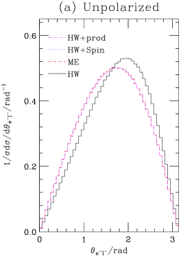
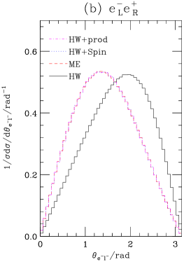
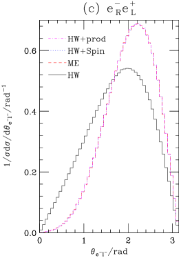
Figure 9: Angle between the lepton produced in $\rm{e}^{+}\rm{e}^{-}\rightarrow\rm{t}\rm{\bar{t}}\rightarrow\rm{b}\rm{\bar{b}}\ell^{+}\nu_{\ell}\ell^{-}\bar{\nu}_{\ell}$ and the incoming electron beam in the laboratory frame for a centre-of-mass energy of 500 GeV with (a) no polarization, (b) negatively polarized electrons and positively polarized positrons and (c) positively polarized electrons and negatively polarized positrons. The solid line shows the default result from HERWIG which treats the production and decay as independent but includes a matrix element for the weak decay of the top, the dashed line gives the full result from the 6-body matrix element, the dotted line the result of the spin correlation algorithm and the dot-dashed line the result of the spin correlation algorithm when the decay matrix for the first quark is neglected.

Here we are mainly concerned with this process as an example of the application of the spin correlation algorithm. In this process in addition to the complications of the $2\to 2$ process, which can have polarization of the incoming particles, there is the problem of correlating the decay of the top quarks with each other. In addition to using the spin density matrix for the top production to perform the decays the decay matrix from the first decay must be used in calculating the spin density matrix used for the decay of the second quark. In the default treatment of this process HERWIG performs the production and decay of the quarks independently but uses the full 3-body matrix element for the quark decays.

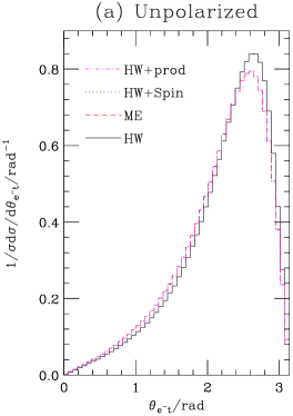
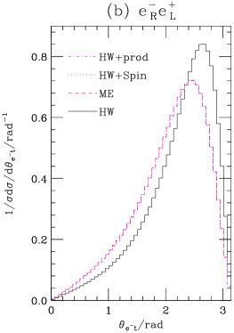
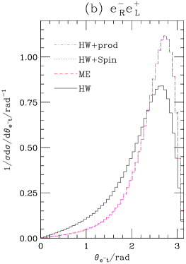
Figure 10: Angle between the lepton and top quark produced in $\rm{e}^{+}\rm{e}^{-}\rightarrow\rm{t}\rm{\bar{t}}\rightarrow\rm{b}\rm{\bar{b}}\ell^{+}\nu_{\ell}\ell^{-}\bar{\nu}_{\ell}$ in the laboratory frame for a centre-of-mass energy of 500 GeV with (a) no polarization, (b) negatively polarized electrons and positively polarized positrons and (c) positively polarized electrons and negatively polarized positrons. The lines are described in the caption of Fig. 9.

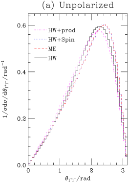
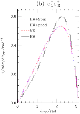
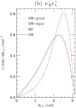
Figure 11: Angle between the leptons produced in $\rm{e}^{+}\rm{e}^{-}\rightarrow\rm{t}\rm{\bar{t}}\rightarrow\rm{b}\rm{\bar{b}}\ell^{+}\nu_{\ell}\ell^{-}\bar{\nu}_{\ell}$ in the laboratory frame for a centre-of-mass energy of 500 GeV  with (a) no polarization, (b) negatively polarized electrons and positively polarized positrons and (c) positively polarized electrons and negatively polarized positrons. The lines are described in the caption of Fig. 9.

Fig. 9 shows the angle of the lepton produced in the top antiquark decay with respect to the incoming electron beam, Fig. 10 shows the angle between the lepton and the top quark and Fig. 11 shows the angle between the lepton and the antilepton. The result of the spin correlation algorithm agrees well with the full 6-body matrix element for all these distributions. Again the major discrepancies between the default treatment in HERWIG and the full result are for the correlation of the direction of the outgoing leptons with the beam and the correlation between the direction of the produced lepton and the second quark in the event.

In addition to the full result of the spin correlation algorithm we have also included the results of the algorithm where the identity is used rather than the decay matrix calculated for the decay of the first quark when calculating the spin density matrix for the decay of the second quark. Neglecting this step of the algorithm still gives good agreement with the matrix-element calculation for the correlation between the direction of the produced lepton and the beam direction, Fig. 9, and the correlation between the direction of the top quark and the lepton, Fig. 10. This is because these correlations mainly depend on the details of the hard production process and not how the first quark decayed.

However, in order to reproduce the result of the matrix element for the angle between the produced lepton and antilepton, Fig. 11, it is essential to include the decay matrix from the first quark as this is a correlation between the two decays. This effect is most noticeable when there is no beam polarization and both possible initial-state spin configurations contribute to the result.

4.4 $\rm{t\bar{t}}$ production in Hadron-Hadron Collisions

Since the discovery of the top quark at the Tevatron there have been a number of studies of spin correlations in top quark pair production for both Run II of the Tevatron and the LHC. There are two processes which contribute to $\rm{t\bar{t}}$ production in hadron collisions

$$\rm{q}\rm{\bar{q}} \longrightarrow \rm{t\bar{t}},$$ (17a)

$$\rm{g}\rm{g} \longrightarrow \rm{t\bar{t}}.$$ (17b)

The $\rm{q}\rm{\bar{q}}$ annihilation process presents no additional complications and is very similar to the $\rm{e}^{+}\rm{e}^{-}$ annihilation we discussed in the previous section.

However the colour flows in the three diagrams for $\rm{t\bar{t}}$ production via gluon scattering, Fig. 12, are very different. It is easiest to extract the colour matrices from the helicity amplitudes and perform the colour sum/averages separately. The colour matrices for the three diagrams, shown in Fig. 12, are

$${C_{t}}^{ab}_{c_{1}c_{2}}= t^{a}_{c_{1}c^{\prime}}t^{b}_{c^{\prime}c_{2}} \ \ \ \ \ \ \ \ \ t\rm{-channel},$$ (18a)

$${C_{u}}^{ab}_{c_{1}c_{2}}= t^{b}_{c_{1}c^{\prime}}t^{a}_{c^{\prime}c_{2}} \ \ \ \ \ \ \ \ \ u\rm{-channel},$$ (18b)

$${C_{s}}^{ab}_{c_{1}c_{2}}= if^{abc}t^{c}_{c_{1}c_{2}} \ \ \ \ \ \ \ \ \ s\rm{-channel},$$ (18c)

where $f^{abc}$ is the $SU(3)$ structure constant, $t^{a}$ is the $SU(3)$ colour matrix in the fundamental representation, ${C_{s,t,u}}^{ab}_{c_{1}c_{2}}$ are the colour matrices for the $s$-, $t$- and $u$-channel colour flows respectively, $a$ is the colour of the first incoming gluon, $b$ is the colour of the second incoming gluon, $c_{1}$ is the colour of the outgoing quark, $c^{\prime}$ is the colour of the intermediate quark and $c_{2}$ is the colour of the outgoing antiquark.

In general the colour flow for diagrams involving the triple gluon vertex, i.e. the $s$-channel diagram, is not unique and can be rewritten in terms of the $t$- and $u$-channel colour flows using the definition of the structure constants

$$if^{abc}t^{c}_{c_{1}c_{2}}=t^{a}_{c_{1}c^{\prime}}t^{b}_{c^{\prime}c_{2}}-t^{b}_{c_{1}c^{\prime}}t^{a}_{c^{\prime}c_{2}},$$ (19)

giving

$${C_{s}}^{ab}_{c_{1}c_{2}}={C_{t}}^{ab}_{c_{1}c_{2}}-{C_{u}}^{ab}_{c_{1}c_{2}},$$ (20)

so that we only have two different colour flows to deal with.

Figure 12: Feynman diagrams for $\rm{g}\rm{g}\rightarrow\rm{t}\rm{\bar{t}}$.

In principle the presence of different colour flows could be a significant problem to the algorithm we are using. We should keep track of the colour flow in the production processes and decays and calculate spin density matrices for each of the flows and sum over them. If the decays have one than one colour flow, in addition to the different colour flows in the hard process, this could lead to an increase in the complexity of the algorithm with the number of final state particles, i.e. the number of colour flows would grow exponentially. However, in both the Standard and Minimal Supersymmetric Standard Models, provided we only consider three-body decays as we are doing, there can only be different colour flows in the hard production process and it is therefore sufficient to replace Eqn. 1 with

$$\sum_{a,b=1,C_{N}}C_{ab}\rho^{1}_{\kappa_{1}\kappa^{\prime}_{1}}\rho^{2}_{\kappa_{2}\kappa^{\prime}_{2}}\mathcal{M}^{a}_{\kappa_{1}\kappa_{2};\lambda_{1}\ldots\lambda_{n}}\mathcal{M}^{b*}_{\kappa^{\prime}_{1}\kappa^{\prime}_{2};\lambda^{\prime}_{1}\ldots\lambda^{\prime}_{n}}\prod_{i=1,n}D^{i}_{\lambda_{i}\lambda^{\prime}_{i}},$$ (21)

where $\mathcal{M}^{a}$ is the matrix element for colour flow $a$, $C_{N}$ is the number of colour flows and $C_{ab}$ is the colour factor for the matrix elements. Eqns. 3 and 4 must also be modified in the same way.

For example in ${\rm t}{\rm\bar{t}}$ collisions

$$C_{tt}= \frac{1}{(N^{2}_{c}-1)^{2}}t^{a}_{c_{1}c^{\prime}}t^{b}_{c^{\prime}c_{2}}t^{a}_{c^{\prime\prime}c_{1}}t^{b}_{c_{2}c^{\prime\prime}} =\phantom{-}\frac{1}{4N_{c}},$$ (22a)

$$C_{uu}= \frac{1}{(N^{2}_{c}-1)^{2}}t^{b}_{c_{1}c^{\prime}}t^{a}_{c^{\prime}c_{2}}t^{b}_{c^{\prime\prime}c_{1}}t^{a}_{c_{2}c^{\prime\prime}} =\phantom{-}\frac{1}{4N_{c}},$$ (22b)

$$C_{tu}= \frac{1}{(N^{2}_{c}-1)^{2}}t^{a}_{c_{1}c^{\prime}}t^{b}_{c^{\prime}c_{2}}t^{b}_{c^{\prime\prime}c_{1}}t^{a}_{c_{2}c^{\prime\prime}} =-\frac{1}{4N_{c}(N^{2}_{c}-1)},$$ (22c)

the colour factor $$C_{ut}=C_{ut}$$.

Another option which would be necessary if the decays have more than one possible colour flow, in for example R-parity violating SUSY models [26, 27], is to select one of the colour flows in the same way as is already done for the production of QCD radiation [28]. In this procedure we would first select a colour flow, $a$, using [28]

$$C_{aa}\rho^{1}_{\kappa_{1}\kappa^{\prime}_{1}}\rho^{2}_{\kappa_{2}\kappa^{\prime}_{2}}\mathcal{M}^{a}_{\kappa_{1}\kappa_{2};\lambda_{1}\ldots\lambda_{n}}\mathcal{M}^{a*}_{\kappa^{\prime}_{1}\kappa^{\prime}_{2};\lambda_{1}\ldots\lambda_{n}}A_{a},$$ (23)

where

$$A_{a}=\frac{\sum_{b,c=1,C_{N}}C_{bc}\rho^{1}_{\kappa_{1}\kappa^{\prime}_{1}}\rho^{2}_{\kappa_{2}\kappa^{\prime}_{2}}\mathcal{M}^{b}_{\kappa_{1}\kappa_{2};\lambda_{1}\ldots\lambda_{n}}\mathcal{M}^{c*}_{\kappa^{\prime}_{1}\kappa^{\prime}_{2};\lambda_{1}\ldots\lambda_{n}}}{\sum_{b=1,C_{N}}C_{bb}\mathcal{M}^{b}_{\kappa_{1}\kappa_{2};\lambda_{1}\ldots\lambda_{n}}\mathcal{M}^{b*}_{\kappa^{\prime}_{1}\kappa^{\prime}_{2};\lambda_{1}\ldots\lambda_{n}}}.$$ (24)

This procedure ensures that the sum over the redefined colour flows reproduces the full result, Eqn. 21. This is used to select the colour flow $a$ for the process and instead of Eqn. 1 to give the distributions of the particles produced in the hard process. The matrix element for the selected colour flow is then used with Eqn. 3 to calculate the spin density matrices for the decays of the particles produced in the hard process.

In models where there is more than one colour flow in a decay we would select the colour flow for the decay and generate the momenta of the decay products according to

$$\rho_{\lambda_{0}\lambda^{\prime}_{0}}C_{aa}\mathcal{M}^{a}_{\lambda_{0};\lambda_{1}\ldots\lambda_{n}}\mathcal{M}^{a*}_{\lambda^{\prime}_{0};\lambda_{1}\ldots\lambda_{n}}E_{a},$$ (25)

where

$$E_{a}=\frac{\sum_{b,c=1,C_{N}}C_{bc}\mathcal{M}^{b}_{\lambda_{0};\lambda_{1}\ldots\lambda_{n}}\mathcal{M}^{c*}_{\lambda^{\prime}_{0};\lambda_{1}\ldots\lambda_{n}}}{\sum_{b=1,C_{N}}C_{bb}\mathcal{M}^{b}_{\lambda_{0};\lambda_{1}\ldots\lambda_{n}}\mathcal{M}^{b*}_{\lambda^{\prime}_{0};\lambda_{1}\ldots\lambda_{n}}}.$$ (26)

The matrix element for the selected colour flow is then used to calculate the spin density matrices for the particles produced in the decay and the decay matrix for this decay once all the particles produced in the decay have been developed.

This approach neglects the interference between the different colour flows in generating the spin correlations, just as they are neglected when generating the QCD radiation. As this procedure is not necessary for the processes we are considering we will use the first procedure in processes where the hard process has more than one colour flow.

There have been many studies of spin correlations in hadron-hadron collisions. In order to study the results of the spin correlation algorithm we have chosen to follow the approach of [29, 30] in which the following observables were defined for top quark pair production followed by $\rm{t}\rightarrow{\rm b}{\rm W}^{+}\rightarrow{\rm b}\rm{q}\rm{\bar{q}}$ and $\rm{\bar{t}}\rightarrow{\rm\bar{b}}{\rm W}^{-}\rightarrow{\rm\bar{b}}\ell^{-}\bar{\nu}$:

$$\mathcal{O}_{1} = \hat{{\bf q}}^{*}_{b}\cdot\hat{{\bf q}}_{\ell^{-}};$$ (27a)

$$\mathcal{O}_{2} = \left(\hat{{\bf q}}^{*}_{b}\cdot\hat{{\bf p}}_{p}\right)\left(\hat{{\bf q}}_{\ell^{-}}\cdot\hat{{\bf p}}_{p}\right);$$ (27b)

$$\mathcal{O}_{3} = \left(\hat{{\bf q}}^{*}_{b}\cdot\hat{{\bf k}}_{t}\right)\left(\hat{{\bf q}}_{\ell^{-}}\cdot\hat{{\bf k}}_{t}\right);$$ (27c)

$$\mathcal{O}_{4} = \frac{1}{2}\left[\left(\hat{{\bf q}}^{*}_{b}\cdot\hat{{\bf p}}_{p}\right)\left(\hat{{\bf q}}_{\ell^{-}}\cdot\hat{{\bf k}}_{t}\right)+\left(\hat{{\bf q}}^{*}_{b}\cdot\hat{{\bf k}}_{t}\right)\left(\hat{{\bf q}}_{\ell^{-}}\cdot\hat{{\bf p}}_{p}\right)\right];$$ (27d)

$$\mathcal{O}_{5} = \mathrm{sgn}\,y_{t}\,\,\mathcal{O}_{4};$$ (27e)

$$\mathcal{O}_{6} = \left(\hat{{\bf p}}_{p}\times\hat{{\bf q}}^{*}_{b}\right)\cdot\left(\hat{{\bf p}}_{p}\times\hat{{\bf q}}_{\ell^{-}}\right)=\mathcal{O}_{1}-\mathcal{O}_{2}.$$ (27f)

All the hatted vectors are unit vectors and the quantities without an asterisk are measured in the laboratory frame, $\hat{{\bf p}}_{p}$ is the beam direction, $\hat{{\bf q}}_{\ell^{-}}$ is the direction of the charged lepton, $\hat{{\bf k}}_{t}$ is the direction of the top quark and $y_{t}$ is the rapidity of the top quark. The asterisked quantities are measured in the top quark rest frame and $\hat{{\bf q}}^{*}_{b}$ is the direction of the bottom quark. In a similar way the quantities $\bar{\mathcal{O}}_{1-6}$ are defined for the charge conjugate decay modes. The observable $\mathcal{O}_{4}$ is zero when integrated over a symmetric rapidity interval which is why the observable $\mathcal{O}_{5}$ is defined.

	$\mathcal{O}$/%			$\bar{\mathcal{O}}$/%
	Full	Spin 1	Spin 2	Full	Spin 1	Spin 2
$\mathcal{O}_{1}$	$\phantom{-}2.46\pm 0.04$	$\phantom{-}2.45\pm 0.02$	$\phantom{-}2.41\pm 0.02$	$\phantom{-}2.42\pm 0.04$	$\phantom{-}2.46\pm 0.02$	$\phantom{-}2.44\pm 0.02$
$\mathcal{O}_{2}$	$\phantom{-}2.94\pm 0.02$	$\phantom{-}2.92\pm 0.01$	$\phantom{-}2.90\pm 0.01$	$\phantom{-}2.91\pm 0.02$	$\phantom{-}2.91\pm 0.01$	$\phantom{-}2.89\pm 0.01$
$\mathcal{O}_{3}$	$\phantom{-}1.68\pm 0.02$	$\phantom{-}1.67\pm 0.01$	$\phantom{-}1.64\pm 0.01$	$\phantom{-}1.67\pm 0.02$	$\phantom{-}1.68\pm 0.01$	$\phantom{-}1.65\pm 0.01$
$\mathcal{O}_{4}$	$\phantom{-}0.03\pm 0.02$	$\phantom{-}0.01\pm 0.01$	$\phantom{-}0.01\pm 0.01$	$-0.01\pm 0.02$	$\phantom{-}0.00\pm 0.01$	$-0.01\pm 0.01$
$\mathcal{O}_{5}$	$\phantom{-}1.95\pm 0.02$	$\phantom{-}1.94\pm 0.01$	$\phantom{-}1.92\pm 0.01$	$\phantom{-}1.92\pm 0.02$	$\phantom{-}1.93\pm 0.01$	$\phantom{-}1.92\pm 0.01$
$\mathcal{O}_{6}$	$-0.48\pm 0.03$	$-0.47\pm 0.02$	$-0.46\pm 0.02$	$-0.49\pm 0.03$	$-0.45\pm 0.02$	$-0.48\pm 0.02$

Table 1: Average values of the observables $\mathcal{O}_{1-6}$ and $\bar{\mathcal{O}}_{1-6}$ at Run II of the Tevatron. The top (antitop) quark was required to have rapidity $|y|<2.0$ and transverse momentum $p_{T}>15$ GeV for the observables $\mathcal{O}_{1-6}$ and $\bar{\mathcal{O}}_{1-6}$, respectively. Spin 1 gives the results of the spin correlation algorithm using Eqn. 21 and spin 2 gives the results of the spin correlation algorithm using Eqn. 23.

The results for these observables at Run II of the Tevatron with a centre-of-mass energy of 2 TeV are shown in Table 1 where for events with $\rm{t}\rightarrow{\rm b}{\rm W}^{+}\rightarrow{\rm b}\rm{q}\rm{\bar{q}}$ and $\rm{\bar{t}}\rightarrow{\rm\bar{b}}{\rm W}^{-}\rightarrow{\rm\bar{b}}\ell^{-}\bar{\nu}$ we have required the top quark to have rapidity $|y_{t}|<2.0$ and transverse momentum $p_{T}>15$ GeV. For the charge conjugate decay modes the antitop quark was required to have rapidity $|y_{\bar{t}}|<2.0$ and transverse momentum $p_{T}>15$ GeV.

The results for the same observables at the LHC with a centre-of-mass energy of 14 TeV are shown in Table 2. For events with $\rm{t}\rightarrow{\rm b}{\rm W}^{+}\rightarrow{\rm b}\rm{q}\rm{\bar{q}}$ and $\rm{\bar{t}}\rightarrow{\rm\bar{b}}{\rm W}^{-}\rightarrow{\rm\bar{b}}\ell^{-}\bar{\nu}$ we have required the top quark to have rapidity $|y_{t}|<3.0$ and transverse momentum $p_{T}>20$ GeV. For the charge conjugate decay modes the antitop quark was required to have rapidity $|y_{\bar{t}}|<3.0$ and transverse momentum $p_{T}>20$ GeV.

	$\mathcal{O}$/%			$\bar{\mathcal{O}}$/%
	Full	Spin 1	Spin 2	Full	Spin 1	Spin 2
$\mathcal{O}_{1}$	$-2.01\pm 0.02$	$-2.04\pm 0.02$	$-2.04\pm 0.02$	$-2.03\pm 0.02$	$-2.04\pm 0.02$	$-2.02\pm 0.02$
$\mathcal{O}_{2}$	$-0.16\pm 0.02$	$-0.16\pm 0.02$	$-0.18\pm 0.02$	$-0.18\pm 0.02$	$-0.19\pm 0.02$	$-0.16\pm 0.02$
$\mathcal{O}_{3}$	$-0.55\pm 0.02$	$-0.56\pm 0.02$	$-0.57\pm 0.01$	$-0.57\pm 0.02$	$-0.59\pm 0.02$	$-0.57\pm 0.01$
$\mathcal{O}_{4}$	$\phantom{-}0.00\pm 0.02$	$-0.01\pm 0.01$	$-0.02\pm 0.01$	$-0.02\pm 0.02$	$\phantom{-}0.00\pm 0.01$	$\phantom{-}0.01\pm 0.01$
$\mathcal{O}_{5}$	$-0.23\pm 0.02$	$-0.25\pm 0.01$	$-0.25\pm 0.01$	$-0.26\pm 0.02$	$-0.28\pm 0.01$	$-0.25\pm 0.01$
$\mathcal{O}_{6}$	$-1.85\pm 0.02$	$-1.87\pm 0.02$	$-1.86\pm 0.01$	$-1.85\pm 0.02$	$-1.85\pm 0.02$	$-1.85\pm 0.01$

Table 2: Average values of the observables $\mathcal{O}_{1-6}$ and $\bar{\mathcal{O}}_{1-6}$ at the LHC. The top (antitop) quark was required to have rapidity $|y|<3.0$ and transverse momentum $p_{T}>20$ GeV for the observables $\mathcal{O}_{1-6}$ and $\bar{\mathcal{O}}_{1-6}$, respectively. Spin 1 gives the results of the spin correlation algorithm using Eqn. 21 and spin 2 gives the results of the spin correlation algorithm using Eqn. 23.

All the results were generated using a top quark mass of 175 GeV and the default parton distribution functions in HERWIG6.3 [10] which are the average of the central and higher gluon leading-order fits of [31].

As can be seen in both Tables 1 and 2 the results of the spin correlation algorithm, with either method of handling the different colour flows, are in good agreement with the result of the 6-body matrix element. The default result from HERWIG for all these observables was consistent with zero. This is because these observables are designed to be sensitive to the spin correlations and zero in the absence of such correlations.

At the Tevatron the most significant of these observables is $\mathcal{O}_{2}$ whereas the observable $\mathcal{O}_{6}$ is the most important at the LHC. At the LHC this is because while the average value of $\mathcal{O}_{1}$ is greater the fluctuations are also greater which gives a greater statistical sensitivity for $\mathcal{O}_{6}$ [29, 30].

4.5 $\rm{e^{+}e^{-}\rightarrow\tilde{\chi}^{+}\tilde{\chi}^{-}}$

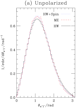
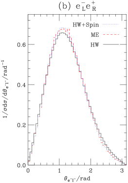
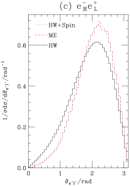
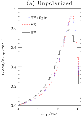
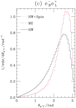
Figure 13: Angle between the lepton produced in $\rm{e}^{+}\rm{e}^{-}\rightarrow\tilde{\chi}^{+}_{1}\tilde{\chi}^{-}_{1}\rightarrow\ell^{+}\nu_{\ell}\tilde{\chi}^{0}_{1}\ell^{-}\bar{\nu}_{\ell}\tilde{\chi}^{0}_{1}$ and the incoming electron beam in the laboratory frame for a centre-of-mass energy of 500 GeV  with (a) no polarization, (b) negatively polarized electrons and positively polarized positrons and (c) positively polarized electrons and negatively polarized positrons. The solid line shows the default result from HERWIG, the dashed line gives the full result from the 6-body matrix element and the dotted line the result of the spin correlation algorithm.

Figure 14: Angle between the leptons produced in $\rm{e}^{+}\rm{e}^{-}\rightarrow\tilde{\chi}^{+}_{1}\tilde{\chi}^{-}_{1}\rightarrow\ell^{+}\nu_{\ell}\tilde{\chi}^{0}_{1}\ell^{-}\bar{\nu}_{\ell}\tilde{\chi}^{0}_{1}$ in the laboratory frame for a centre-of-mass energy of 500 GeV  with (a) no polarization, (b) negatively polarized electrons and positively polarized positrons and (c) positively polarized electrons and negatively polarized positrons. The solid line shows the default result from HERWIG, the dashed line gives the full result from the 6-body matrix element and the dotted line the result of the spin correlation algorithm.

So far we have only considered processes in which the fermions have small widths relative to their masses, the next-to-lightest neutralino in most SUSY models has a width of less than one hundred MeV and the top quark width is about one GeV. We can therefore neglect the width in top quark and neutralino production processes. In the limit that the width of the decaying fermion can be neglected the helicity amplitudes for the production processes, including the fermion decays, can be factorized into a production and decay helicity amplitude. The spin correlation algorithm is in good agreement with the full matrix element in these cases.

However, if the decaying fermion is not on mass-shell the process cannot be factorized and the result of the spin correlation algorithm may not give such good agreement with the $2\to n$ body matrix elements. This should not be a serious problem because even in SUSY models the electroweak gauginos tend to have widths of at most a few GeV, for the heavier gauginos. The gluino width tends to be larger, but the gluino is heavier, and therefore the effect is the same. The particles which usually have the largest widths in most SUSY models are the squarks and these effects can be taken into account because they are scalars.

In order to study the effects of the widths of the decaying fermions it is easiest to study chargino production in ${\rm e}^{+}{\rm e}^{-}$ collisions because this allows us to consider the production of $\tilde{\chi}^{\pm}_{1}\tilde{\chi}^{\mp}_{2}$ in which the lighter chargino has a very small width and the heavier chargino has a much greater width. Spin and polarization effects in chargino pair production in ${\rm e}^{+}{\rm e}^{-}$ collisions have been previously considered in [2, 4].

We used the following SUSY parameters in this study: $M_{1}=78$ GeV, $M_{2}=158$ GeV, $\mu=330$ GeV, $\tan\beta=3$, $M_{L_{L}}=171$ GeV and $M_{e_{R}}=180$ GeV, where the soft SUSY breaking masses for the gauginos and the $\mu$ parameter are given at the electroweak scale, $M_{L_{L}}$ is the soft SUSY breaking mass for the lepton doublet at the electroweak scale and $M_{e_{R}}$ is the soft SUSY breaking mass for the right-handed electron singlet at the electroweak scale.

At this point the lightest neutralino mass is $M_{\tilde{\chi}^{0}_{1}}=71.6$ GeV, the lightest chargino mass is $M_{\tilde{\chi}^{+}_{1}}=127.8$ GeV, the heaviest chargino mass is $M_{\tilde{\chi}^{+}_{2}}=357.6$ GeV, the sneutrino mass is $M_{\tilde{\nu}_{L}}=160.9$ GeV, the left selectron mass is $M_{\tilde{\ell}_{L}}=176.1$ GeV and the right selectron mass is $M_{\tilde{\ell}_{R}}=184.2$ GeV. The width of the lightest chargino is $\Gamma_{\tilde{\chi}^{+}_{1}}=73$ MeV and the heaviest chargino is $\Gamma_{\tilde{\chi}^{+}_{2}}=2.9$ GeV.

This point was chosen to have a negligible lightest chargino width and a variety of leptonic decay modes, i.e. $\tilde{\chi}^{+}_{2}\rightarrow\ell^{+}\tilde{\nu}_{L}\rightarrow\ell^{+}\ell^{-}\tilde{\chi}^{0}_{1}$, $\tilde{\chi}^{+}_{2}\rightarrow\tilde{\ell}^{+}_{L}\nu\rightarrow\ell^{+}\ell^{-}\tilde{\chi}^{0}_{1}$ and $\tilde{\chi}^{+}_{2}\rightarrow\tilde{\chi}^{0}_{1}W^{+}\rightarrow\ell^{+}\ell^{-}\tilde{\chi}^{0}_{1}$, of the heaviest chargino.

It is interesting to first consider $\tilde{\chi}^{+}_{1}\tilde{\chi}^{-}_{1}$ production, where there are no width effects. Fig. 14 shows the angle between the lepton produced in ${\rm e}^{+}{\rm e}^{-}\rightarrow\tilde{\chi}^{+}_{1}\tilde{\chi}^{-}_{1}\rightarrow\tilde{\chi}^{0}_{1}\ell^{+}\nu\tilde{\chi}^{0}_{1}\ell^{-}\bar{\nu}$ and the beam direction and Fig. 14 shows the angle between the lepton and the antilepton. As before there is good agreement between the full result and the spin correlation algorithm.

In a Monte Carlo simulation however we need to include the widths of the unstable particles as these widths can potentially be measured. When we include the effect of the width in the spin correlation algorithm we have two choices. We can use the off-mass shell momentum in Eqn. 38 for the spinor of the massive particle together with either the physical mass of the particle or the off-shell mass of the particle.

In the first case this gives

$$\sum_{\lambda}u_{\lambda}(p)\bar{u}_{\lambda}(p)=p\!\!\!\!\!\not\>\>\!+m+\frac{l\!\!\!\!\!\not\>\>\!}{2p\cdot l}(m^{2}-p^{2}),$$ (28)

where $p$ is the off-shell four-momentum, $m$ is the on-shell mass and $l$ is the reference vector. This form reduces to the correct spin sum if the particle is on-mass shell. However for off-mass shell particles there is an additional component which depends on the choice of the reference vector and is related to how off-mass shell the particle is.

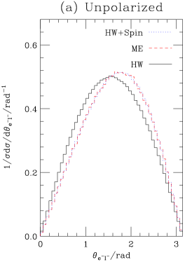
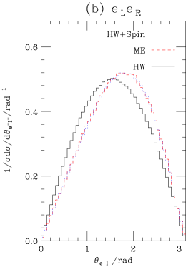
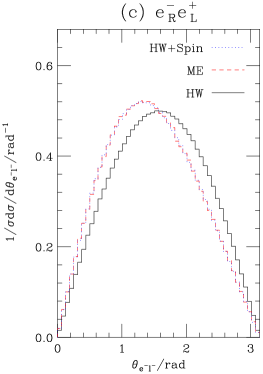
Figure 15: Angle between the lepton produced in $\rm{e}^{+}\rm{e}^{-}\rightarrow\tilde{\chi}^{+}_{1}\tilde{\chi}^{-}_{2}\rightarrow\ell^{+}\nu_{\ell}\tilde{\chi}^{0}_{1}\ell^{-}\bar{\nu}_{\ell}\tilde{\chi}^{0}_{1}$ and the incoming electron beam in the laboratory frame for a centre-of-mass energy of 500 GeV  with (a) no polarization, (b) negatively polarized electrons and positively polarized positrons and (c) positively polarized electrons and negatively polarized positrons. The solid line shows the default result from HERWIG, the dashed line gives the full result from the 6-body matrix element and the dotted line the result of the spin correlation algorithm.

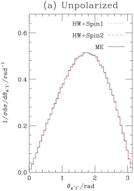
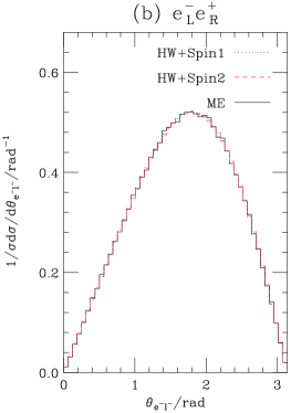
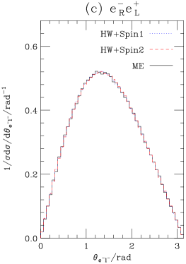
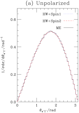
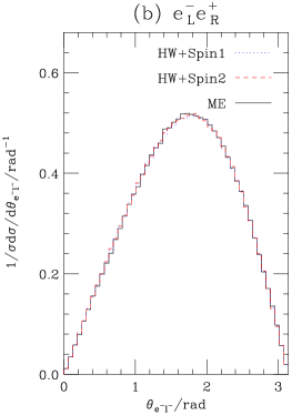
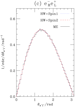
Figure 16: Angle between the lepton produced in $\rm{e}^{+}\rm{e}^{-}\rightarrow\tilde{\chi}^{+}_{1}\tilde{\chi}^{-}_{2}\rightarrow\ell^{+}\nu_{\ell}\tilde{\chi}^{0}_{1}\ell^{-}\bar{\nu}_{\ell}\tilde{\chi}^{0}_{1}$ and the incoming electron beam in the laboratory frame for a centre-of-mass energy of 500 GeV  with (a) no polarization, (b) negatively polarized electrons and positively polarized positrons and (c) positively polarized electrons and negatively polarized positrons. The physical $\tilde{\chi}^{\pm}_{2}$ width was used. The solid line shows the full result, the dotted line shows the result of the spin correlation algorithm with the physical mass and the dashed line shows the result of the spin correlation algorithm with the off-shell mass of the chargino.

Figure 17: Angle between the lepton produced in $\rm{e}^{+}\rm{e}^{-}\rightarrow\tilde{\chi}^{+}_{1}\tilde{\chi}^{-}_{2}\rightarrow\ell^{+}\nu_{\ell}\tilde{\chi}^{0}_{1}\ell^{-}\bar{\nu}_{\ell}\tilde{\chi}^{0}_{1}$ and the incoming electron beam in the laboratory frame for a centre-of-mass energy of 500 GeV  with (a) no polarization, (b) negatively polarized electrons and positively polarized positrons and (c) positively polarized electrons and negatively polarized positrons. Ten times the physical $\tilde{\chi}^{\pm}_{2}$ width was used. The lines are described in the caption on Fig. 17.

If we choose to use the off-shell mass rather than the physical mass in Eqn. 38 we obtain

$$\sum_{\lambda}u_{\lambda}(p)\bar{u}_{\lambda}(p)=p\!\!\!\!\!\not\>\>\!+m_{\rm off},$$ (29)

where $m_{\rm off}$ is the off-shell mass. Here the result again fails to reproduce the correct result by an amount which depends on the how far off-shell the particle is, however it does not depend on the arbitrary reference vector. We have studied the effects of both these choices.

We considered $\tilde{\chi}^{\pm}_{1}\tilde{\chi}^{\mp}_{2}$ production followed by the decay of the lightest chargino $\tilde{\chi}^{\pm}_{1}\rightarrow\ell^{\pm}\nu\tilde{\chi}^{0}_{1}$ via a three-body decay and heaviest chargino $\tilde{\chi}^{\pm}_{1}\rightarrow{\rm W}^{\pm}\tilde{\chi}^{0}_{1}\rightarrow\ell^{\pm}\nu\tilde{\chi}^{0}_{1}$. The angle of the lepton produced in the $\tilde{\chi}^{\pm}_{2}$ decay with respect to the beam direction is shown in Fig. 15 where we have neglected the widths of the decaying charginos.

We then considered the effect of including the width of the decay chargino. Fig. 17 shows the result for the physical width of the heaviest chargino and Fig. 17 shows the effect of increasing the width by a factor of ten.

These results show that there is still good agreement between the full result and the spin correlation algorithm even when particles with fairly large widths are included, despite the potential problems. The result does not significantly depend on the choice of the spinor for the unstable particle and therefore we will use the second choice in order to avoid any dependence on the reference vector used to define the particle’s spin.

5 Tau Decays

So far we have only discussed spin correlations in the SM for the top quark which is the only quark which decays before hadronization. However spin correlations can also be important for the decay of the tau. The tau will undergo a weak decay to a tau neutrino and either an electron/muon and its associated antineutrino or hadrons. Due to the relatively small mass of the tau only a small number of hadrons can be produced in its decay.

The matrix elements for the leptonic decay of the tau and many of the hadronic decay modes are known, either theoretically or from experimental measurements of the distributions of the decay products. The helicity of the decaying tau can affect the distribution of the decay products. There is a package TAUOLA [32] which includes the matrix elements for the leptonic and many of the hadronic modes and includes the helicity of the decaying tau.

In order to implement the algorithm we have suggested in full for tau decays we would need to completely rewrite the TAUOLA package to use the spin density matrices for the decays and return the decay matrix after performing the decays. Given the number of decay modes and the sophisticated treatment of the decays in TAUOLA this would be a major project and is beyond the scope of this study.

However as TAUOLA makes use of the helicity of the decay tau to perform the decays we can use the diagonal entries of the spin density matrices, which give the probability the tau has a given helicity, to select the helicity of the decaying tau.

6 Including Correlations with the Parton Shower

Given the similarities between the algorithm we are using in order to include spin correlations from heavy particle decays and the algorithm of [5, 6, 7, 8] for spin correlations in the QCD parton shower it should be possible to produce an algorithm which includes both effects, i.e. correctly includes correlations from both heavy particle decays and in the QCD shower.

In order to construct such an algorithm it is helpful to first review the algorithm of [5, 6, 7, 8] for correlations in the QCD parton shower. The full algorithm is given for both forward and backward evolution in [7]. The algorithm proceeds in the following way:

1. The momenta of the particles in the hard collision process are generated according to Eqn. 1.

2. One of the outgoing partons is chosen at random and given a spin density matrix according to Eqn. 3.

3. The type of the branching, $i\to j+k$, together with the azimuthal angle $\phi$ and momentum fraction $z$, are generated according to

   $$\rho^{i}_{\lambda_{i}\lambda^{\prime}_{i}}V^{jk}_{\lambda_{i}\lambda_{j}\lambda_{k}}(z,\phi)V^{jk*}_{\lambda^{\prime}_{i}\lambda^{\prime}_{j}\lambda^{\prime}_{k}}(z,\phi)D^{j}_{\lambda_{j}\lambda^{\prime}_{j}}D^{k}_{\lambda_{k}\lambda^{\prime}_{k}},$$ (30)

   where $V^{jk}_{\lambda_{i}\lambda_{j}\lambda_{k}}(z,\phi)$ is the splitting function for the branching given the helicities, $\lambda_{i},\lambda_{j},\lambda_{k}$ of the partons, $\rho^{i}_{\lambda_{i}\lambda^{\prime}_{i}}$ is the spin density matrix of the parton entering the vertex and $D^{j}_{\lambda_{j}\lambda^{\prime}_{j}}$ is the decay matrix for the partons leaving the vertex. As before in the first stage of the algorithm the decay matrix is taken to be $D^{j}_{\lambda_{j}\lambda^{\prime}_{j}}=\delta_{\lambda_{j}\lambda^{\prime}_{j}}$.

4. One of the outgoing partons is selected to be developed and a spin density matrix calculated for this parton using

   $$\rho^{j}_{\lambda_{j}\lambda^{\prime}_{j}}=\frac{1}{N_{\rho\rm{QCD}}}\rho^{i}_{\lambda_{i}\lambda^{\prime}_{i}}V^{jk}_{\lambda_{i}\lambda_{j}\lambda_{k}}(z,\phi)V^{jk*}_{\lambda^{\prime}_{i}\lambda^{\prime}_{j}\lambda^{\prime}_{k}}(z,\phi)D^{k}_{\lambda_{k}\lambda^{\prime}_{k}},$$ (31)

   where the normalization

   $$N_{\rho\rm{QCD}}=\rho^{i}_{\lambda_{i}\lambda^{\prime}_{i}}V^{jk}_{\lambda_{i}\lambda_{j}\lambda_{k}}(z,\phi)V^{jk*}_{\lambda^{\prime}_{i}\lambda_{j}\lambda^{\prime}_{k}}(z,\phi)D^{k}_{\lambda_{k}\lambda^{\prime}_{k}},$$ (32)

   is chosen so that the spin density matrix has unit trace. This procedure is repeated until the parton to be developed reaches the cut-off scale. As before the decay matrix for this parton is then set to $\delta_{\lambda_{i}\lambda^{\prime}_{i}}$.

5. Another parton from the branching which produced the parton which reached the cut-off scale is now developed with a spin density matrix calculated for this parton using Eqn. 31. When all the outgoing partons in a branching have been developed a decay matrix for that branching is calculated using

   $$D^{i}_{\lambda_{i}\lambda^{\prime}_{i}}=\frac{1}{N_{D{\rm QCD}}}V^{jk}_{\lambda_{i}\lambda_{j}\lambda_{k}}(z,\phi)V^{jk*}_{\lambda^{\prime}_{i}\lambda^{\prime}_{j}\lambda^{\prime}_{k}}(z,\phi)D^{j}_{\lambda_{j}\lambda^{\prime}_{j}}D^{k}_{\lambda_{k}\lambda^{\prime}_{k}},$$ (33)

   where the normalization

   $$N_{D{\rm QCD}}=V^{jk}_{\lambda_{i}\lambda_{j}\lambda_{k}}(z,\phi)V^{jk*}_{\lambda_{i}\lambda^{\prime}_{j}\lambda^{\prime}_{k}}(z,\phi)D^{j}_{\lambda_{j}\lambda^{\prime}_{j}}D^{k}_{\lambda_{k}\lambda^{\prime}_{k}}$$ (34)

   is chosen so that the trace of the decay matrix is one. The other outgoing partons from the previous branching are now developed with a spin density matrix calculated using Eqn. 31 and the calculated decay matrix rather than the identity for those partons which have been developed.

6. This procedure is repeated until the hard process is reached. Another outgoing parton is selected and a spin density matrix calculated for it using Eqn. 3 and the calculated decay matrices for those particles which have already been developed rather than the identity. Step three of the algorithm is then performed for this particle. This procedure is repeated until all the outgoing particles in the hard process have been developed.

This is the algorithm for the forward evolution of outgoing time-like partons. A similar algorithm [7] can be used to develop the incoming space-like partons. This algorithm starts the development with a decay matrix calculated according to

$$D_{\kappa_{j}\kappa^{\prime}_{j}}=\frac{1}{N_{I}}\rho^{i\neq j}_{\kappa_{i}\kappa^{\prime}_{i}}\mathcal{M}_{\kappa_{i}\kappa_{j};\lambda_{1}\ldots\lambda_{n}}\mathcal{M}^{*}_{\kappa^{\prime}_{i}\kappa^{\prime}_{j};\lambda^{\prime}_{1}\ldots\lambda^{\prime}_{n}}\prod_{k=1,n}D^{k}_{\lambda_{k}\lambda^{\prime}_{k}}.$$ (35)

The normalization

$$N_{I}=\rho^{i\neq j}_{\kappa_{i}\kappa^{\prime}_{i}}\mathcal{M}_{\kappa_{i}\kappa_{j};\lambda_{1}\ldots\lambda_{n}}\mathcal{M}^{*}_{\kappa^{\prime}_{i}\kappa_{j};\lambda^{\prime}_{1}\ldots\lambda^{\prime}_{n}}\prod_{k=1,n}D^{i}_{\lambda_{k}\lambda^{\prime}_{k}}$$ (36)

is again chosen such that the decay matrix has unit trace. We will not discuss the details of this backward evolution algorithm here, it is described in [7]. It is sufficient to note that when a space-like parton has been completely developed the algorithm returns a spin density matrix for the developed parton. So the full algorithm for spin correlations in the QCD shower is that the outgoing time-like partons are developed according to the algorithm described above and then using the decay matrices returned by this algorithm the incoming space-like partons are developed according to the algorithm of [7].

In order to treat the spin correlations the best possible approach would be as follows:

1. The momenta of the particles in the hard collision are generated according to Eqn. 1.

2. One of the outgoing particles is selected at random and a spin density matrix calculated for it according to Eqn. 3.

3. If the particle is colourless and unstable step four is performed, if the particle is coloured step five is performed, otherwise the decay matrix for this particle is set to $\delta_{\lambda_{i}\lambda^{\prime}_{i}}$, another particle selected and this step repeated.

4. The decay mode of the particle is selected according to the branching ratios and the momenta of the particles produced in the $n-$body decay generated according to Eqn. 5.

   1. A particle from this decay is selected and a spin density matrix calculated for it using Eqn. 6.

   2. If this particle is unstable and colourless we perform step four.

   3. If the particle is coloured step five is performed.

   4. If the particle is stable and colourless its decay matrix is set to $\delta_{\lambda_{i}\lambda^{\prime}_{i}}$ and another particle from the decay which produced it is selected to be developed. Once all the particles in a given decay have been developed a decay matrix is calculated for the decay using Eqn. 8 and another particle from the decay or branching which produced this particle selected to be developed. A spin density matrix is calculated for the development of this particle with the calculated decay matrix rather than the identity for those particles which have been developed. Step three is then performed for this particle.

5. If the particle is coloured and has not reached the cut-off scale its branching, $i\rightarrow jk$, is generated according to Eqn. 30. If the parton has reached the cut-off scale then:

   1. If the particle is stable its decay matrix is set to $\delta_{\lambda_{i}\lambda^{\prime}_{i}}$ and another particle from the branching or decay which produced this parton selected to be developed. If all the particles in a branching have been developed a decay matrix for the parton which branches is calculated using Eqn. 33 and another particle from the decay or branching which produced it selected to be developed. Similarly if all the particles in a decay have been developed a decay matrix is calculated for the decay using Eqn. 8 and another particle from the decay or branching which produced it selected to be developed. A spin density matrix is calculated for the development of this particle with the calculated decay matrix rather than the identity for those particles which have been developed. Step three is then performed for this particle.

   2. If the particle is unstable step four is performed for the particle.

   If a branching occurs the following procedure is performed:

   1. One of the outgoing particles is selected to be developed and a spin density matrix calculated using Eqn. 31.

   2. Step five is then performed for this particle.

6. Eventually this algorithm will return a decay matrix for one of the particles produced in the hard process. If there are still outgoing particles which have not been developed then another outgoing particle is selected to be developed and step two performed for this particle.

7. If all the outgoing particles have been developed then one of the incoming particles is selected and a decay matrix calculated using Eqn. 35. The algorithm described in [7] is used to develop the incoming particle. This is repeated until all the incoming particles have been developed.

As with both the QCD and heavy particle decay algorithms we have already described the decay matrix for any particle which has not been developed is taken to be $\delta_{\lambda_{i}\lambda^{\prime}_{i}}$.

While this algorithm is the most efficient way in which to include the spin correlations it presents problems in generating the parton shower. This is because the parton shower algorithm needs to produce the QCD radiation from all the particles produced in the same hard collision or decay at the same time. There are several reasons for this:

1. The scale used for the strong coupling constant in the parton shower algorithm depends on the energy of the collision, or mass of the decaying particle.

2. In the angular-ordered parton shower used in HERWIG [33, 34, 35] the maximum angle for the emission of QCD radiation from a parton is determined by the direction of its colour partner, which is defined by the colour flow in the hard process or decay.

3. The parton-shower algorithm does not conserve energy and momentum. Therefore after the radiation from all the partons in a process has been generated the momenta of the resulting jets must be adjusted in order to ensure energy and momentum conservation.

We need to consider an algorithm in which this is possible. While this algorithm will be less efficient in the way it implements the spin correlations it should prove much easier to interface with the QCD parton shower. The algorithm will proceed in the following way:

1. First the algorithm for spin correlations in the both the initial- and final-state QCD parton shower is run as before.

2. Then if there are any unstable particles produced one of them is selected at random and a spin density matrix calculated in the following way:

   1. The decay matrices for the other undecayed particles are set to $\delta_{\lambda_{i}\lambda^{\prime}_{i}}$.

   2. We then use the matrix elements of all the vertices to produce the decay matrices of the particles in the hard process, apart from the particle which produced the one we have selected, and the spin density matrices for the incoming partons. This should be straightforward as these decay matrices will have already been calculated by the QCD spin correlation algorithm.

   3. Using these decay matrices and Eqn. 3 we construct the spin density matrix for the parton which initiated the shower which produced the selected particle.

   4. We then move down the branch that produced the particle we have selected using Eqn. 31 and the decay matrices which have already been calculated for the side-branches.

   5. Eventually we will reach the particle we have selected with a spin density matrix calculated according to Eqn. 31.

3. The decay mode of this particle is selected according to the branching ratios and the momenta of the decay products generated according to Eqn. 5.

4. If any coloured particles are produced the QCD parton-shower algorithm is run. If the decay produces unstable particles we perform steps two and three for this decay, using Eqn. 6 rather than Eqn. 3.

5. Eventually we will perform a decay in which only stable particles are produced. When this happens we set the decay matrices for the stable particles to $\delta_{\lambda_{i}\lambda^{\prime}_{i}}$ and use the decay matrices calculated by the QCD algorithm and Eqn. 8 to calculate a decay matrix for this decay.

6. We then select another unstable particle produced in the previous decay, or the parton shower initiated by that decay, and repeat the procedure with the decay matrix calculated from Eqn. 8 for the particles for which the decays have been performed. If there are no further unstable particles to decay we use Eqn. 8 to calculate the decay matrix and move up the chain.

7. Eventually we will reach a particle which was produced in the parton shower after the hard collision. We then select another unstable particle and repeat the process using the calculated decay matrix rather than the identity for those particles which have been decayed.

8. This procedure is repeated until all the unstable particles produced in the parton shower initiated by the hard process have been decayed.

This procedure is more complicated as additional spin density and decay matrices have to be stored and recalculated but it should prove easier to implement the parton shower with this procedure.

The implementation of either of the algorithms we have described in this section would involve a major rewrite of the HERWIG, or any other, event generator. As there are currently projects under way to rewrite the current generation of FORTRAN event generators in C++[36, 37] it would be pointless to undertake this rewrite. Hopefully, one of the algorithms we have described here can be implemented in the next generation of C++ event generators.

7 Conclusions

We have shown that it is possible to construct an algorithm for spin correlations in a Monte Carlo event generator that both allows us to generate the production and decay of the heavy particles as separate steps and has a complexity which only grows linearly with the number of final-state particles. An additional advantage of this algorithm is that we only have to calculate the helicity amplitudes for $2\to 2$ collision processes and, at least for the processes we have studied, at most three body decays rather than the calculation of $n-$body matrix elements.

This algorithm gives results that are in good agreement with the full calculations of the $n-$body matrix elements for all the processes we have studied. In the appendix we have given the helicity amplitudes necessary to implement this algorithm in a Monte Carlo event generator. These results have been incorporated into the HERWIG event generator and will be available in the next version.

Finally, we have proposed an algorithm to include both the spin correlations in heavy particle decays which we have considered here as well the correlations in and between jets which are already included in the HERWIG event generator. This algorithm, which would require a major rewrite of the current generation of FORTRAN event generators, can hopefully be included in the next generation of C++ event generators which are currently being written [36, 37].

Appendix A Spinor Conventions

In general we will use the conventions of [38, 39] for the spinors in the helicity amplitudes for the matrix elements. However it is more convenient for us to define

$$s_{\lambda}(p_{1},p_{2})=\bar{u}_{\lambda}(p_{1})u_{-\lambda}(p_{2}),$$ (37)

rather than the $s$ and $t$ functions of [38].

We will use the following notation for massive fermions,

$$u(p,\lambda) = \phantom{-}\frac{1}{\sqrt{2p\cdot\ell}}\left(p\!\!\!\!\!\not\>\>\!+m\right)u_{-\lambda}(l),$$ (38a)

$$v(p,\lambda) = -\frac{1}{\sqrt{2p\cdot\ell}}\left(p\!\!\!\!\!\not\>\>\!-m\right)u_{-\lambda}(l),$$ (38b)

where $p$ is the four-momentum of the fermion, $m$ is its mass, $\lambda$ is the spin of the fermion and $\ell^{\mu}$ is a light-like four-vector. This choice for the massive fermions both reproduces the standard spin sums for Dirac particles

$$\sum_{\lambda}u_{\lambda}(p)\bar{u}_{\lambda}(p) = \left(p\!\!\!\!\!\not\>\>\!+m\right),$$ (39a)

$$\sum_{\lambda}v_{\lambda}(p)\bar{v}_{\lambda}(p) = \left(p\!\!\!\!\!\not\>\>\!-m\right),$$ (39b)

and the additional spin sums required in SUSY models which have Majorana fermions [40]

$$\sum_{\lambda}u_{\lambda}(p)v^{T}_{\lambda}(p) = \left(p\!\!\!\!\!\not\>\>\!+m\right)C^{T},$$ (40a)

$$\sum_{\lambda}\bar{u}^{T}_{\lambda}(p)\bar{v}_{\lambda}(p) = C^{-1}\left(p\!\!\!\!\!\not\>\>\!-m\right),$$ (40b)

$$\sum_{\lambda}\bar{v}^{T}_{\lambda}(p)\bar{u}_{\lambda}(p) = C^{-1}\left(p\!\!\!\!\!\not\>\>\!+m\right),$$ (40c)

$$\sum_{\lambda}v_{\lambda}(p)u^{T}_{\lambda}(p) = \left(p\!\!\!\!\!\not\>\>\!-m\right)C^{T}.$$ (40d)

Given this choice it is useful to define

$$p^{\mu}=\tilde{p}^{\mu}+\ell^{\mu},$$ (41)

where $\tilde{p}^{2}=0$ and $\ell^{2}=0$. In this notation the spin vector for the particle is given by

$$s^{\mu}=\frac{1}{m}(\tilde{p}^{\mu}-l^{\mu}).$$ (42)

The choice of the spin vector is completely arbitrary in our case provided that we are consistent, i.e. we use the same choice for the production and decay of the particle.

In the expressions for the amplitudes it will often be convenient to express the results in terms of the function

$$F(\lambda_{1},p_{1},k,m,\lambda_{2},p_{2})=\bar{u}_{\lambda_{1}}(p_{1})\left(k\!\!\!\!\!\!\not\>\>\!\,+m\right)u_{\lambda_{2}}(p_{2}),$$ (43)

where $p_{1,2}$ are massless four vectors, $\lambda_{1,2}$ are helicities and $k$ is an arbitrary four-vector. This function can be evaluated in terms of spinors as follows [39]

$$F(\lambda,p_{1},k,m,-\lambda,p_{2}) = ms_{\lambda}(p_{1},p_{2})$$ (44a)

$$F(\lambda,p_{1},k,m,\phantom{-}\lambda,p_{2}) = s_{\lambda}(p_{1},\tilde{k})s_{-\lambda}(\tilde{k},p_{2}),$$ (44b)

where

$$\tilde{k}^{\mu}=k^{\mu}-\frac{k^{2}}{2k\cdot p_{2}}p^{\mu}_{2}.$$ (45)

We will use the same notation as [38] for the polarization vectors of the massless gauge bosons

$$\epsilon_{\lambda}^{\mu}(p)=\frac{1}{2\sqrt{p\cdot l}}\bar{u}_{\lambda}(p)\gamma^{\mu}u_{\lambda}(l),$$ (46)

where $p$ is the four-momentum of the gauge boson and $l$ is an arbitrary light-like four-vector which is not collinear to $p$. The choice of this light-like vector corresponds to the making a choice of gauge and therefore we can either chose $l^{\mu}$ in order to simplify the calculation or vary it in order to test the gauge invariance of the results.

The choice of the representation for the polarizations of the massive gauge bosons is discussed in [38]. However, as this representation basically replaces the gauge boson with two massless fermions, into which the boson decays, we will not include any on-shell massive gauge bosons but replace them with their decay products.

Appendix B Couplings

In this section we will give the couplings for both the SM and MSSM in a format suitable for use in the helicity amplitudes for both the production and decay of the particles.

In order to specify the matrix elements we need the couplings for the vertices involved. In general we have taken the form of a vector-fermion-fermion vertex to be

$$ia^{\lambda}\gamma^{\mu}P_{\lambda}.$$ (47)

The couplings of the gauge bosons to the Standard Model fermions are given in Table 3 where $e$ is the magnitude of the electron’s charge, $g$ the weak coupling and $\theta_{W}$ the weak mixing angle.

$a_{{\rm B}{\rm f}{\rm\bar{f}}}$	$a_{{\rm B}{\rm f}{\rm\bar{f}}}^{+}$	$a_{{\rm B}{\rm f}{\rm\bar{f}}}^{-}$
$a_{{\rm W}{\rm f}{\rm\bar{f^{\prime}}}}$	0	$-\frac{g}{\sqrt{2}}V_{{\rm f}{\rm f}^{\prime}}$
$a_{{\rm Z}{\rm f}{\rm\bar{f}}}$	$\frac{ge_{\rm f}\sin^{2}\theta_{W}}{\cos\theta_{W}}$	$-\frac{g}{\cos\theta_{W}}(t^{3}_{\rm f}-e_{\rm f}\sin^{2}\theta_{W})$

Table 3: Couplings of the SM fermions to the gauge bosons, where $t^{3}_{\rm f}$ is the weak isospin of the fermion and $e_{\rm f}$ is its electric charge in units of the magnitude of the electron’s charge. The isospin partner of the fermion f is denoted by ${\rm f^{\prime}}$. $V_{{\rm f}{\rm f}^{\prime}}$ is the relevant element of the Cabibbo-Kobayashi-Maskawa (CKM) matrix.

In the MSSM there are a lot more couplings which must be specified and this is complicated by the mixing of the particles involved. The physical electroweak gauginos are mixings of the interaction eigenstates. There are mixing matrices: $N$ for the neutralinos; and $U$ and $V$ for the charginos. In general our conventions for the mixing of the gauginos follow those of [40, 41, 42]. In performing the diagonalization to go from the interaction to mass eigenstates there is a choice: we can either take the mixing matrices to be complex, in which case the masses are positive; or the mixing matrices to be real and let the masses be positive or negative, in which case we must redefine the field $\tilde{\chi}\rightarrow\gamma_{5}\tilde{\chi}$ if the mass is negative [40, 41, 42]. As the calculations will be implemented numerically it is more convenient to deal with real mixing matrices and we must therefore keep track of the sign of the gaugino masses and change the sign of certain couplings. We will denote the sign of the mass of the $i$th neutralino by $\epsilon_{i}$ and the $i$th chargino by $\eta_{i}$. The couplings of the gauge bosons to the gauginos of the MSSM are given in Table 4.

$a_{{\rm B}\tilde{\chi}\tilde{\chi}}$	$a^{+}_{{\rm B}\tilde{\chi}\tilde{\chi}}$	$a^{-}_{{\rm B}\tilde{\chi}\tilde{\chi}}$
$a_{{\rm Z}\tilde{\chi}^{+}_{i}\tilde{\chi}^{-}_{j}}$	$-\frac{g}{\cos\theta_{W}}\left(U^{*}_{i1}U_{j1}+\frac{1}{2}U^{*}_{i2}U_{j2}-\delta_{ij}\sin^{2}\theta_{W}\right)$	$-\frac{g\eta_{i}\eta_{j}}{\cos\theta_{W}}\left(V_{i1}V^{*}_{j1}+\frac{1}{2}V_{i2}V^{*}_{j2}-\delta_{ij}\sin^{2}\theta_{W}\right)$
$a_{{\rm Z}\tilde{\chi}^{0}_{i}\tilde{\chi}^{0}_{j}}$	$\frac{g}{2\cos\theta_{W}}\left(N^{*}_{i3}N_{j3}-N^{*}_{i4}N_{j4}\right)$	$-\epsilon_{i}\epsilon_{j}a^{+*}_{Z\tilde{\chi}^{0}_{i}\tilde{\chi}^{0}_{j}}$
$a_{{\rm W}\tilde{\chi}^{0}_{i}\tilde{\chi}^{-}_{j}}$	$g\left(\frac{1}{\sqrt{2}}N^{*}_{i3}U_{j2}+N^{*}_{i2}U_{j1}\right)$	$-g\epsilon_{i}\eta_{j}\left(\frac{1}{\sqrt{2}}N_{i4}V^{*}_{j2}-N_{i2}V^{*}_{j1}\right)$

Table 4: Couplings of the gauge bosons to the electroweak gauginos. The mixing matrices for the neutralinos, $N$, and charginos, $U$ and $V$, are defined in the notation of [40, 41, 42].

$a_{{\rm B}\mathrm{\tilde{f}}\mathrm{\tilde{f}}^{*}}$		$a_{{\rm B}\mathrm{\tilde{f}}\mathrm{\tilde{f}}^{*}}$
$a_{{\rm Z}{\rm\tilde{q}}_{i\alpha}{\rm\tilde{q}}^{*}_{i\beta}}$	$-\frac{g}{\cos\theta_{W}}\left(t^{3}_{q}Q^{i}_{1\alpha}Q^{i*}_{1\beta}-e_{q}\sin^{2}\theta_{W}\delta_{\alpha\beta}\right)$	$a_{{\rm W}{\rm\tilde{d}}_{i\alpha}{\rm\tilde{u}}^{*}_{i\beta}}$	$-\frac{g}{\sqrt{2}}Q^{2i-1}_{1\alpha}Q^{2i*}_{1\beta}$
$a_{{\rm Z}\tilde{\ell}_{i\alpha}\tilde{\ell}^{*}_{i\beta}}$	$-\frac{g}{\cos\theta_{W}}\left(t^{3}_{\ell}L^{i}_{1\alpha}L^{i*}_{1\beta}-e_{\ell}\sin^{2}\theta_{W}\delta_{\alpha\beta}\right)$	$a_{{\rm W}\tilde{\ell}_{i\alpha}\tilde{\nu}_{iL}}$	$-\frac{g}{\sqrt{2}}L^{2i-1}_{1\alpha}$
$a_{\gamma\mathrm{\tilde{f}}\mathrm{\tilde{f}}^{*}}$	$-iee_{\rm f}$

Table 5: Couplings of the sfermions to the electroweak gauge bosons. These couplings are taken from [40]. The flavour of the sfermion is denoted by $i$ and $\alpha,\beta$ gives the mass eigenstate.

In general there can be mixing between all the sfermions with the same electric and colour charges. However, we will only consider mixing between the left and right scalar partners of the same fermion. We use the same convention as the HERWIG event generator for this left/right mixing, this is discussed in [26, 27, 16]. In this notation the mixing matrix for the squarks is $Q^{i}_{\alpha\beta}$, where $i=1-6$ for the d, u, s, c, b and t squarks, $\alpha$ is the left/right eigenstate and $\beta$ is the mass eigenstate. Similarly the mixing matrix for the sleptons is $L^{i}_{\alpha\beta}$, where $i=1-6$ for the $\rm{e}$, $\nu_{\rm{e}}$, $\mu$, $\nu_{\mu}$, $\tau,\nu_{\tau}$ sleptons, $\alpha$ is the left/right eigenstate and $\beta$ is the mass eigenstate.

The form of the boson-scalar-scalar vertex is taken to be

$$ia(p+p^{\prime})^{\mu},$$ (48)

where the momentum $p$ is taken to be flowing into the vertex and $p^{\prime}$ is taken to be flowing out of the vertex. The couplings of the sfermions to the electroweak gauge bosons are given in Table 5 and of the Higgs bosons to the gauge bosons in Table 6.

$a_{{\rm B}{\rm H}{\rm H}}$		$a_{{\rm B}{\rm H}{\rm H}}$
$a_{{\rm W}^{\pm}{\rm H}^{\pm}{\rm h}^{0}}$	$\mp\frac{g}{2}\cos(\beta-\alpha)$	$a_{{\rm W}^{\pm}{\rm H}^{\pm}{\rm A}^{0}}$	$-i\frac{g}{2}$
$a_{{\rm W}^{\pm}{\rm H}^{\pm}{\rm H}^{0}}$	$\pm\frac{g}{2}\sin(\beta-\alpha)$	$a_{{\rm Z}{\rm A}^{0}{\rm h}^{0}}$	$-i\frac{g\cos(\beta-\alpha)}{2\cos\theta_{W}}$
$a_{{\rm Z}{\rm A}^{0}{\rm H}^{0}}$	$i\frac{g\sin(\beta-\alpha)}{2\cos\theta_{W}}$

Table 6: Couplings of the Higgs bosons to the electroweak gauge bosons. These couplings are taken from [43, 44]. The angle $\alpha$ is the mixing between interaction and mass eigenstates of the two neutral scalar Higgs bosons.

The form of the scalar-fermion-fermion vertex is

$$ia^{\lambda}P_{\lambda}.$$ (49)

The couplings of the neutralinos to the sfermions are given in Table 7, of the charginos to the sfermions in Table 11 and of the gluino to the squarks in Table 11. In order to define the couplings of the sfermions to the neutralinos it is useful to define the following functions

$$S^{+}_{{\rm f}\tilde{\chi}^{0}_{i}} = -N^{\prime}_{i1}ee_{\rm f}+N^{\prime}_{i2}a^{+}_{{\rm Z}{\rm f}{\rm\bar{f}}},$$ (50a)

$$S^{-}_{{\rm f}\tilde{\chi}^{0}_{i}} = \phantom{-}N^{\prime*}_{i1}ee_{\rm f}-N^{\prime*}_{i2}a^{-}_{{\rm Z}{\rm f}{\rm\bar{f}}},$$ (50b)

for the couplings of the gaugino part of the neutralinos to the fermions. The functions

$$H_{{\rm f}\tilde{\chi}^{0}_{i}} = \left\{\begin{array}[]{cl}\frac{gm_{\rm f}N_{i4}}{2M_{\mathrm{W}}\sin\beta}&\rm{for\ up-type\ quarks\ and\ neutrinos,}\\ &\\ \frac{gm_{\rm f}N_{i3}}{2M_{\mathrm{W}}\cos\beta}&\rm{for\ down-type\ quarks\ and\ charged\ leptons,}\\ \end{array}\right.$$ (54)

give the couplings of the fermions to the Higgsino part of the neutralinos.

$a_{\tilde{\chi}^{0}_{l}\mathrm{\tilde{f}}{\rm f}}$	$a^{+}_{\tilde{\chi}^{0}_{l}\mathrm{\tilde{f}}{\rm f}}$	$a^{-}_{\tilde{\chi}^{0}_{l}\mathrm{\tilde{f}}{\rm f}}$
$a_{\tilde{\chi}^{0}_{l}{\rm\tilde{q}}_{i\alpha}{\rm q}_{i}}$	$-\sqrt{2}\epsilon_{l}\left(Q^{i}_{1\alpha}H_{{\rm q}_{i}\tilde{\chi}^{0}_{l}}+Q^{i}_{2\alpha}S^{+}_{{\rm q}_{i}\tilde{\chi}^{0}_{l}}\right)$	$-\sqrt{2}\left(Q^{i}_{2\alpha}H^{*}_{{\rm q}_{i}\tilde{\chi}^{0}_{l}}+Q^{i}_{1\alpha}S^{-}_{{\rm q}_{i}\tilde{\chi}^{0}_{l}}\right)$
$a_{\tilde{\chi}^{0}_{l}\tilde{\ell}_{i\alpha}\ell_{i}}$	$-\sqrt{2}\epsilon_{l}\left(L^{i}_{1\alpha}H_{\ell_{i}\tilde{\chi}^{0}_{l}}+L^{i}_{2\alpha}S^{+}_{\ell_{i}\tilde{\chi}^{0}_{l}}\right)$	$-\sqrt{2}\left(L^{i}_{2\alpha}H^{*}_{\ell_{i}\tilde{\chi}^{0}_{l}}+L^{i}_{1\alpha}S^{-}_{\ell_{i}\tilde{\chi}^{0}_{l}}\right)$

Table 7: Couplings of the neutralinos to the sfermions and fermions. The flavour of the sfermion is denoted by $i$ and $\alpha$ gives the mass eigenstate.

$a_{\tilde{\chi}^{+}_{l}{\rm\tilde{f}}{\rm f}}$	$a^{+}_{\tilde{\chi}^{+}_{i}{\rm\tilde{f}}{\rm f}}$	$a^{-}_{\tilde{\chi}^{+}_{i}{\rm\tilde{f}}{\rm f}}$
$a_{\tilde{\chi}^{+}_{l}{\rm\tilde{u}}_{i\alpha}{\rm d}_{i}}$	$\frac{g}{\sqrt{2}M_{W}\cos\beta}m_{{\rm d}_{i}}U_{l2}Q^{2i}_{1\alpha}$	$-g\eta_{l}\left(V^{*}_{l1}Q^{2i}_{1\alpha}-\frac{1}{\sqrt{2}M_{W}\sin\beta}m_{{\rm u}_{i}}V^{*}_{l2}Q^{2i}_{2\alpha}\right)$
$a_{\tilde{\chi}^{+}_{l}{\rm\tilde{d}}_{i\alpha}{\rm u}_{i}}$	$\frac{g\eta_{l}}{\sqrt{2}M_{W}\sin\beta}m_{{\rm u}_{i}}V_{l2}Q^{2i-1}_{1\alpha}$	$-g\left(U^{*}_{l1}Q^{2i-1}_{1\alpha}-\frac{1}{\sqrt{2}M_{W}\cos\beta}m_{{\rm d}_{i}}U^{*}_{l2}Q^{2i-1}_{2\alpha}\right)$
$a_{\tilde{\chi}^{+}_{l}\tilde{\nu}_{iL}\ell_{i}}$	$\frac{g}{\sqrt{2}M_{W}\cos\beta}m_{\ell_{i}}U_{l2}$	$-g\eta_{l}V^{*}_{l1}$
$a_{\tilde{\chi}^{+}_{l}\tilde{\ell}_{i\alpha}\nu_{i}}$	$0$	$-g\left(U^{*}_{l1}L^{2i-1}_{1\alpha}-\frac{1}{\sqrt{2}M_{W}\cos\beta}m_{\ell_{i}}U^{*}_{l2}L^{2i-1}_{2\alpha}\right)$

Table 8: Couplings of the sfermions to the charginos. The generation of the sfermion is given by $i$ and $\alpha$ is its mass eigenstate.

$a_{{\rm\tilde{g}}{\rm\tilde{q}}{\rm q}}$	$a^{+}_{{\rm\tilde{g}}{\rm\tilde{q}}{\rm q}}$	$a^{-}_{{\rm\tilde{g}}{\rm\tilde{q}}{\rm q}}$
$a_{{\rm\tilde{g}}{\rm\tilde{u}}_{i}{\rm u}_{i}}$	$g_{s}\sqrt{2}Q^{2i}_{2\alpha}$	$-g_{s}\sqrt{2}Q^{2i}_{1\alpha}$
$a_{{\rm\tilde{g}}{\rm\tilde{d}}_{i}{\rm d}_{i}}$	$g_{s}\sqrt{2}Q^{2i-1}_{2\alpha}$	$-g_{s}\sqrt{2}Q^{2i-1}_{1\alpha}$

Table 9: Couplings of the squarks to the gluino. The flavour of the squark is given by $i$ and $\alpha$ is the mass eigenstate of the squark.

$a_{{\rm H}\tilde{\chi}\tilde{\chi}}$	$a^{+}_{{\rm H}\tilde{\chi}\tilde{\chi}}$	$a^{-}_{{\rm H}\tilde{\chi}\tilde{\chi}}$
$a_{{\rm h}_{0}\tilde{\chi}^{0}_{i}\tilde{\chi}^{0}_{j}}$	$g\left(Q^{\prime\prime}_{ij}\sin\alpha+S^{\prime\prime}_{ij}\cos\alpha\right)$	$g\left(Q^{\prime\prime*}_{ji}\sin\alpha+S^{\prime\prime*}_{ji}\cos\alpha\right)$
$a_{{\rm H}_{0}\tilde{\chi}^{0}_{i}\tilde{\chi}^{0}_{j}}$	$g\left(S^{\prime\prime}_{ij}\sin\alpha-Q^{\prime\prime}_{ij}\cos\alpha\right)$	$g\left(S^{\prime\prime*}_{ji}\sin\alpha-Q^{\prime\prime*}_{ji}\cos\alpha\right)$
$a_{{\rm A}_{0}\tilde{\chi}^{0}_{i}\tilde{\chi}^{0}_{j}}$	$-ig\left(Q^{\prime\prime}_{ij}\sin\beta-S^{\prime\prime}_{ij}\cos\beta\right)$	$ig\left(Q^{\prime\prime*}_{ji}\sin\beta-S^{\prime\prime*}_{ji}\cos\beta\right)$
$a_{{\rm h}_{0}\tilde{\chi}^{+}_{i}\tilde{\chi}^{-}_{j}}$	$g\left(Q_{ij}\sin\alpha-S_{ij}\cos\alpha\right)$	$g\left(Q^{*}_{ji}\sin\alpha-S^{*}_{ji}\cos\alpha\right)$
$a_{{\rm H}_{0}\tilde{\chi}^{+}_{i}\tilde{\chi}^{-}_{j}}$	$-g\left(Q_{ij}\cos\alpha+S_{ij}\sin\alpha\right)$	$-g\left(Q^{*}_{ji}\cos\alpha+S^{*}_{ji}\sin\alpha\right)$
$a_{{\rm A}_{0}\tilde{\chi}^{+}_{i}\tilde{\chi}^{-}_{j}}$	$-ig\left(Q_{ij}\sin\beta+S_{ij}\cos\beta\right)$	$ig\left(Q^{*}_{ji}\sin\beta+S^{*}_{ji}\cos\beta\right)$
$a_{{\rm H}^{-}\tilde{\chi}^{0}_{i}\tilde{\chi}^{-}_{j}}$	$-gQ^{\prime R}_{ij}\sin\beta$	$-gQ^{\prime L}_{ij}\cos\beta$

Table 10: Couplings of the MSSM Higgs bosons to the gauginos.

$a_{{\rm H}{\rm f}{\rm\bar{f}}}$	$a^{+}_{{\rm H}{\rm f}{\rm\bar{f}}}$	$a^{-}_{{\rm H}{\rm f}{\rm\bar{f}}}$	$a_{{\rm H}{\rm f}{\rm\bar{f}}}$	$a^{+}_{{\rm H}{\rm f}{\rm\bar{f}}}$	$a^{-}_{{\rm H}{\rm f}{\rm\bar{f}}}$
$a_{{\rm h}^{0}{\rm u}_{i}{\rm\bar{u}}_{i}}$	$-\frac{gm_{{\rm u}_{i}}\cos\alpha}{2M_{\mathrm{W}}\sin\beta}$	$a^{+}_{{\rm h}^{0}{\rm u}_{i}{\rm\bar{u}}_{i}}$	$a_{{\rm H}^{0}{\rm u}_{i}{\rm\bar{u}}_{i}}$	$-\frac{gm_{{\rm u}_{i}}\sin\alpha}{2M_{\mathrm{W}}\sin\beta}$	$a^{+}_{{\rm H}^{0}{\rm u}_{i}{\rm\bar{u}}_{i}}$
$a_{{\rm h}^{0}{\rm d}_{i}{\rm\bar{d}}_{i}}$	$\frac{gm_{{\rm d}_{i}}\sin\alpha}{2M_{\mathrm{W}}\cos\beta}$	$a^{+}_{{\rm h}^{0}{\rm d}_{i}{\rm\bar{d}}_{i}}$	$a_{{\rm H}^{0}{\rm d}_{i}{\rm\bar{d}}_{i}}$	$-\frac{gm_{{\rm d}_{i}}\cos\alpha}{2M_{\mathrm{W}}\cos\beta}$	$a^{+}_{{\rm H}^{0}{\rm d}_{i}{\rm\bar{d}}_{i}}$
$a_{{\rm h}^{0}\ell_{i}\bar{\ell}_{i}}$	$\frac{gm_{\ell_{i}}\sin\alpha}{2M_{\mathrm{W}}\cos\beta}$	$a^{+}_{{\rm h}^{0}\ell_{i}\bar{\ell}_{i}}$	$a_{{\rm H}^{0}\ell_{i}\bar{\ell}_{i}}$	$-\frac{gm_{\ell_{i}}\cos\alpha}{2M_{\mathrm{W}}\cos\beta}$	$a^{+}_{{\rm H}^{0}\ell_{i}\bar{\ell}_{i}}$
$a_{{\rm A}^{0}{\rm u}_{i}{\rm\bar{u}}_{i}}$	$i\frac{gm_{{\rm u}_{i}}\cot\beta}{2M_{\mathrm{W}}}$	$-a^{+}_{{\rm A}^{0}{\rm u}_{i}{\rm\bar{u}}_{i}}$	$a_{{\rm H}^{+}{\rm u}_{i}{\rm\bar{d}}_{i}}$	$\frac{gm_{{\rm d}_{i}}\tan\beta}{\sqrt{2}M_{\mathrm{W}}}$	$\frac{gm_{{\rm u}_{i}}\cot\beta}{\sqrt{2}M_{\mathrm{W}}}$
$a_{{\rm A}^{0}{\rm d}_{i}{\rm\bar{d}}_{i}}$	$i\frac{gm_{{\rm d}_{i}}\tan\beta}{2M_{\mathrm{W}}}$	$-a^{+}_{{\rm A}^{0}{\rm d}_{i}{\rm\bar{d}}_{i}}$	$a_{{\rm H}^{+}\nu_{i}\bar{\ell}_{i}}$	$\frac{gm_{\ell_{i}}\tan\beta}{\sqrt{2}M_{\mathrm{W}}}$	$0$
$a_{{\rm A}^{0}\ell_{i}\bar{\ell}_{i}}$	$i\frac{gm_{\ell_{i}}\tan\beta}{2M_{\mathrm{W}}}$	$-a^{+}_{{\rm A}^{0}\ell_{i}\bar{\ell}_{i}}$

Table 11: Couplings of the MSSM Higgs bosons to the Standard Model fermions.

The couplings of the Higgs boson of the MSSM to the electroweak gauginos are given in Table 11 where

$$Q_{ij} = \frac{\eta_{i}}{\sqrt{2}}V_{i1}U_{j2},$$ (55a)

$$S_{ij} = \frac{\eta_{i}}{\sqrt{2}}V_{i2}U_{j1},$$ (55b)

$$Q^{\prime L}_{ij} = \eta_{j}\left[N_{i4}V_{j1}+\frac{1}{\sqrt{2}}V_{j2}\left(N_{i2}+N_{i1}\tan\theta_{W}\right)\right],$$ (55c)

$$Q^{\prime R}_{ij} = \epsilon_{i}\left[N_{i3}U_{j1}-\frac{1}{\sqrt{2}}U_{j2}\left(N_{i2}+N_{i1}\tan\theta_{W}\right)\right],$$ (55d)

$$Q^{\prime\prime}_{ij} = \frac{\epsilon_{i}}{2}\left[N_{i3}\left(N_{j2}-N_{j1}\tan\theta_{W}\right)+N_{j3}\left(N_{i2}-N_{i1}\tan\theta_{W}\right)\right],$$ (55e)

$$S^{\prime\prime}_{ij} = \frac{\epsilon_{i}}{2}\left[N_{i4}\left(N_{j2}-N_{j1}\tan\theta_{W}\right)+N_{j4}\left(N_{i2}-N_{i1}\tan\theta_{W}\right)\right],$$ (55f)

taken from [43].

The couplings of the Higgs bosons to the Standard Model fermions are given in Table 11.

We also need the couplings of the MSSM Higgs bosons to gauge boson pairs. The coupling has the form $iag^{\mu\nu}$ with the couplings $gM_{\mathrm{W}}\sin(\beta-\alpha)$ for the lightest Higgs boson to a pair of either W or Z bosons. The coupling of the heavier scalar Higgs boson is $gM_{\mathrm{W}}\cos(\beta-\alpha)$.

Appendix C Production Matrix Elements

There are a large number of both SM and MSSM processes implemented in most general purpose Monte Carlo event generators. In the case of the Standard Model most of these processes do not involve the production of the top quark or tau lepton which are the only fermions for which the spin correlations are relevant. There are a number of other processes involving three or four particles in the final state, for example production of a gauge or Higgs boson in association with a $\rm{t}\rm{\bar{t}}$ pair which have much smaller cross sections.

A large number of the MSSM production processes involve the production of a pair of scalar particles, and therefore we do not need the matrix elements for these processes. This leaves a reasonably small number of $2\to 2$ processes for which we must calculate the matrix elements.

In this section we will first present the helicity amplitude expressions for all the Feynman diagrams which occur in the $2\to 2$ processes we are considering. These amplitudes can then be combined to give all the matrix elements we will need. In all the matrix elements $p_{i}$ and $m_{i}$ are the four-momentum and mass of the $i$th particle, respectively. The vector $l_{i}$ is used to define the direction of the particle’s spin and $\lambda_{i}$ is the helicity of the $i$th particle.

C.1 Feynman Diagrams

C.1.1 Diagram 1

Figure 18: Feynman diagram for $\rm{f}(p_{1})\rm{\bar{f}}(p_{2})\rightarrow\rm{f^{\prime}}(p_{3})\rm{\bar{f^{\prime}}}(p_{4})$ via $s$-channel gauge boson exchange, where ${\rm f}$ and ${\rm f^{\prime}}$ can be any fermion.

The Feynman diagram for $\rm{f}\rm{\bar{f}}\rightarrow\rm{f^{\prime}}\rm{\bar{f^{\prime}}}$ via $s$-channel gauge boson exchange is shown in Fig. 18. The form of the first and second vertices are taken to be $ia^{\lambda}\gamma^{\mu}P_{\lambda}$ and $ib^{\lambda}\gamma^{\mu}P_{\lambda}$. The amplitude is given by

$$\mathcal{M} = -\frac{\delta_{\lambda_{1}\lambda_{2}}a^{\lambda_{1}}}{\sqrt{p_{3}\cdot l_{3}p_{4}\cdot l_{4}}}\frac{1}{\hat{s}-M_{B}^{2}+i\Gamma_{B}M_{B}}$$

$$\left[\phantom{+}b^{-\lambda_{1}}F(-\lambda_{3},l_{3},p_{3},m_{3},\phantom{-}\lambda_{1},p_{1})F(\phantom{-}\lambda_{1},p_{2},p_{4},-m_{4},-\lambda_{4},l_{4})\right.$$

$$\left.\ +b^{\lambda_{1}\phantom{-}}F(-\lambda_{3},l_{3},p_{3},m_{3},-\lambda_{1},p_{2})F(-\lambda_{1},p_{1},p_{4},-m_{4},-\lambda_{4},l_{4})\right],$$

where $\hat{s}=(p_{1}+p_{2})^{2}$, $M_{B}$ is the mass of the exchanged boson and $\Gamma_{B}$ is the width of the exchanged boson. The masses of the incoming particles have been neglected. If we wish to consider both the outgoing particles to be fermions rather than a fermion and an antifermion, in for example gaugino pair production, the sign of $\lambda_{4}$ should be changed.

C.1.2 Diagram 2

Figure 19: Feynman diagram for $\rm{f}(p_{1})\rm{\bar{f}}(p_{2})\rightarrow\rm{f^{\prime}}(p_{3})\rm{\bar{f^{\prime}}}(p_{4})$ via $t$-channel scalar exchange, where ${\rm f}$ and ${\rm f^{\prime}}$ can be any fermion.

The Feynman diagram for $\rm{f}\rm{\bar{f}}\rightarrow\rm{f^{\prime}}\rm{\bar{f^{\prime}}}$ via $t$-channel scalar exchange is shown in Fig. 19. We will take the form of the upper vertex to be $ia^{\lambda}P_{\lambda}$ and the lower vertex to be $ib^{\lambda}P_{\lambda}$. The matrix element is given by

$$\mathcal{M} = -\frac{a^{\lambda_{1}}b^{-\lambda_{2}}}{2\sqrt{p_{3}\cdot l_{3}p_{4}\cdot l_{4}}}\frac{1}{\hat{t}-M^{2}_{\Phi}}$$

$$F(-\lambda_{3},l_{3},p_{3},m_{3},\lambda_{1},p_{1})F(\lambda_{2},p_{2},p_{4},-m_{4},-\lambda_{4},l_{4}),$$

where $\hat{t}=(p_{1}-p_{3})^{2}$ and $M_{\Phi}$ is the mass of the exchanged scalar. The incoming particles have been taken to be massless. As before if we wish to regard particle four as a fermion rather than an antifermion the sign of its helicity should be changed.

C.1.3 Diagram 3

Figure 20: Feynman diagram for $\rm{f}(p_{1})\rm{\bar{f}}(p_{2})\rightarrow\rm{f^{\prime}}(p_{3})\rm{\bar{f^{\prime}}}(p_{4})$ via $u$-channel scalar exchange, where ${\rm f}$ and ${\rm f^{\prime}}$ can be any fermion.

The Feynman diagram for $\rm{f}\rm{\bar{f}}\rightarrow\rm{f^{\prime}}\rm{\bar{f^{\prime}}}$ via $u$-channel scalar exchange is shown in Fig. 20. As for the previous diagram we will take the form of the upper vertex to be $ia^{\lambda}P_{\lambda}$ and the lower vertex to be $ib^{\lambda}P_{\lambda}$. The amplitude is given by

$$\mathcal{M} = \frac{a^{\lambda_{1}}b^{-\lambda_{2}}}{2\sqrt{p_{3}\cdot l_{3}p_{4}\cdot l_{4}}}\frac{1}{\hat{u}-M^{2}_{\Phi}}$$

$$F(\lambda_{4},l_{4},p_{4},m_{4},\lambda_{1},p_{1})F(p_{2},\lambda_{2},p_{3},-m_{3},\lambda_{3},l_{3}),$$

where $\hat{u}=(p_{1}-p_{4})^{2}$, $M_{\Phi}$ is the mass of the exchanged sfermion and we have assumed the incoming particles are massless. The sign of $\lambda_{4}$ should be changed if we wish to consider both outgoing particles as fermions.

C.1.4 Diagram 4

Figure 21: Feynman diagram for $\rm{g}(p_{1})\rm{g}(p_{2})\rightarrow\rm{f}(p_{3})\rm{\bar{f}}(p_{4})$ via $t$-channel fermion exchange.

The Feynman diagram for $\rm{g}\rm{g}\rightarrow\rm{f}\rm{\bar{f}}$ via $t$-channel fermion exchange is shown in Fig. 21. In this case the form of the gluon-quark-quark vertex is taken to be $-ig_{s}\gamma^{\mu}$, where $g_{s}$ is the strong coupling. The colour matrices are not included as it is easier to handle the colour sums/averages for the diagrams separately. This would also allow us to use the same matrix elements for fermion-antifermion production in photon-photon collisions by replacing the strong coupling with the electric charge. The matrix element is given by

$$\mathcal{M} = \frac{g_{s}^{2}}{2\sqrt{p_{1}\cdot l_{1}p_{2}\cdot l_{2}p_{3}\cdot l_{3}p_{4}\cdot l_{4}}}\frac{1}{\hat{t}-m^{2}_{3}}$$

$$\left[\phantom{+}F(-\lambda_{3},l_{3},p_{3},m_{3},\phantom{-}\lambda_{1},l_{1})\right.$$

$$\ \ \ \ \ \ \ \ \ \ \ \ \ \ \ \ \ \left\{\phantom{+}F(\phantom{-}\lambda_{1},p_{1},p_{2}-p_{4},m_{3},\phantom{-}\lambda_{2},l_{2})F(\phantom{-}\lambda_{2},p_{2},p_{4},-m_{4},-\lambda_{4},l_{4})\right.$$

$$\ \ \ \ \ \ \ \ \ \ \ \ \ \ \ \ \ \ \left.\,+F(\phantom{-}\lambda_{1},p_{1},p_{2}-p_{4},m_{3},-\lambda_{2},p_{2})F(-\lambda_{2},l_{2},p_{4},-m_{4},-\lambda_{4},l_{4})\right\}$$

$$\ +F(-\lambda_{3},l_{3},p_{3},m_{3},-\lambda_{1},p_{1})$$

$$\ \ \ \ \ \ \ \ \ \ \ \ \ \ \ \ \ \left\{\phantom{+}F(-\lambda_{1},l_{1},p_{2}-p_{4},m_{3},\phantom{-}\lambda_{2},l_{2})F(\phantom{-}\lambda_{2},p_{2},p_{4},-m_{4},-\lambda_{4},l_{4})\right.$$

$$\ \ \ \ \ \ \ \ \ \ \ \ \ \ \ \ \ \,\left.\left.\,+F(-\lambda_{1},l_{1},p_{2}-p_{4},m_{3},-\lambda_{2},p_{2})F(-\lambda_{2},l_{2},p_{4},-m_{4},-\lambda_{4},l_{4})\right\}\right].$$

As before if we wish to regard the outgoing antifermion as a fermion, in for example gluino pair production, then we must change the sign of $\lambda_{4}$.

C.1.5 Diagram 5

Figure 22: Feynman diagram for $\rm{g}(p_{1})\rm{g}(p_{2})\rightarrow\rm{f}(p_{3})\rm{\bar{f}}(p_{4})$ via $u$-channel fermion exchange.

The Feynman diagram for $\rm{g}\rm{g}\rightarrow\rm{f}\rm{\bar{f}}$ via $u$-channel fermion exchange is shown in Fig. 22. As with the previous diagram we have not included the colour matrices in the expression for the helicity amplitude. In this case the form of the gluon-quark-quark vertex is taken to be $-ig_{s}\gamma^{\mu}$. The matrix element is given by

$$\mathcal{M} = -\frac{g_{s}^{2}}{2\sqrt{p_{1}\cdot l_{1}p_{2}\cdot l_{2}p_{3}\cdot l_{3}p_{4}\cdot l_{4}}}\frac{1}{\hat{u}-m^{2}_{3}}$$

$$\left[\phantom{+}F(-\lambda_{3},l_{3},p_{3},m_{3},\phantom{-}\lambda_{2},l_{2})\right.$$

$$\ \ \ \ \ \ \ \ \ \ \ \ \ \ \ \ \ \left\{\phantom{+}F(\phantom{-}\lambda_{2},p_{2},p_{1}-p_{4},m_{3},\phantom{-}\lambda_{1},l_{1})F(\phantom{-}\lambda_{1},p_{1},p_{4},-m_{4},-\lambda_{4},l_{4})\right.$$

$$\ \ \ \ \ \ \ \ \ \ \ \ \ \ \ \ \ \,\left.\,+F(\phantom{-}\lambda_{2},p_{2},p_{1}-p_{4},m_{3},-\lambda_{1},p_{1})F(-\lambda_{1},l_{1},p_{4},-m_{4},-\lambda_{4},l_{4})\right\}$$

$$+F(-\lambda_{3},l_{3},p_{3},m_{3},-\lambda_{2},p_{2})$$

$$\ \ \ \ \ \ \ \ \ \ \ \ \ \ \ \ \ \,\left\{\phantom{+}F(-\lambda_{2},l_{2},p_{1}-p_{4},m_{3},\phantom{-}\lambda_{1},l_{1})F(\phantom{-}\lambda_{1},p_{1},p_{4},-m_{4},-\lambda_{4},l_{4})\right.$$

$$\ \ \ \ \ \ \ \ \ \ \ \ \ \ \ \ \ \,\left.\left.\,+F(-\lambda_{2},l_{2},p_{1}-p_{4},m_{3},-\lambda_{1},p_{1})F(-\lambda_{1},l_{1},p_{4},-m_{4},-\lambda_{4},l_{4})\right\}\right].$$

As before if we wish to regard the outgoing antifermion as a fermion, in for example gluino pair production, then we must change the sign of $\lambda_{4}$. The sign of this matrix element has been changed in order to simplify the combination of the matrix elements with the colour factors.

C.1.6 Diagram 6

Figure 23: Feynman diagram for $\rm{g}(p_{1})\rm{g}(p_{2})\rightarrow\rm{f}(p_{3})\rm{\bar{f}}(p_{4})$ via $s$-channel gluon exchange.

The Feynman diagram for $\rm{g}\rm{g}\rightarrow\rm{f}\rm{\bar{f}}$ via $s$-channel gluon exchange is shown in Fig. 23. In this case the form gluon-quark-quark vertex is taken to be $-ig_{s}\gamma^{\mu}$ and the triple gluon vertex to be $ig_{s}\left[(p_{1}-p_{2})^{\gamma}g^{\alpha\beta}+(p_{1}+2p_{2})^{\alpha}g^{\beta\gamma}-(2p_{1}+p_{2})^{\beta}g^{\alpha\gamma}\right]$, where $p_{1},\alpha$, $p_{2},\beta$ and $p_{1}+p_{2},\gamma$ are the momenta and Lorentz indices of the three gluons. The colour matrices are not included in the expression for the amplitude in order to allow us to use the same matrix element for both quark and gluino production. The matrix element is given by

$$\mathcal{M} = \frac{g_{s}^{2}}{4\sqrt{p_{1}\cdot l_{1}p_{2}\cdot l_{2}p_{3}\cdot l_{3}p_{4}\cdot l_{4}}}\frac{1}{\hat{s}}$$

$$\left[\left(\phantom{+}\delta_{\lambda_{1}-\lambda_{2}}s_{\lambda_{1}}(p_{1},l_{2})s_{-\lambda_{1}}(p_{2},l_{1})+\delta_{\lambda_{1}\lambda_{2}}s_{\lambda_{1}}(p_{1},p_{2})s_{-\lambda_{1}}(l_{2},l_{1})\right)\right.$$

$$\ \ \ \ \ \ \ \ \ \ \ \ \ \ \ \left(\phantom{-}F(-\lambda_{3},l_{3},p_{3},m_{3},\lambda,p_{1})F(\lambda,p_{1},p_{4},-m_{4},-\lambda_{4},l_{4})\right.$$

$$\ \ \ \ \ \ \ \ \ \ \ \ \ \ \ \,\left.\,-F(-\lambda_{3},l_{3},p_{3},m_{3},\lambda,p_{2})F(\lambda,p_{2},p_{4},-m_{4},-\lambda_{4},l_{4})\right)$$

$$+2s_{\lambda_{1}}(p_{1},p_{2})s_{-\lambda_{1}}(p_{2},l_{1})$$

$$\ \ \ \ \ \ \ \ \ \ \ \ \ \ \ \left(\phantom{+}F(-\lambda_{3},l_{3},p_{3},m_{3},\phantom{-}\lambda_{2},l_{2})F(\phantom{-}\lambda_{2},p_{2},p_{4},-m_{4},-\lambda_{4},l_{4})\right.$$

$$\ \ \ \ \ \ \ \ \ \ \ \ \ \ \ \,\left.\,+F(-\lambda_{3},l_{3},p_{3},m_{3},-\lambda_{2},p_{2})F(-\lambda_{2},l_{2},p_{4},-m_{4},-\lambda_{4},l_{4})\right)$$

$$-2s_{\lambda_{2}}(p_{2},p_{1})s_{-\lambda_{2}}(p_{1},l_{2})$$

$$\ \ \ \ \ \ \ \ \ \ \ \ \ \ \ \left(\phantom{+}F(-\lambda_{3},l_{3},p_{3},m_{3},\phantom{-}\lambda_{1},l_{1})F(\phantom{-}\lambda_{1},p_{1},p_{4},-m_{4},-\lambda_{4},l_{4})\right.$$

$$\ \ \ \ \ \ \ \ \ \ \ \ \ \ \ \,\left.\left.\,+F(-\lambda_{3},l_{3},p_{3},m_{3},-\lambda_{1},p_{1})F(-\lambda_{1},l_{1},p_{4},-m_{4},-\lambda_{4},l_{4})\right)\right].$$

As before if we wish to regard the outgoing antifermion as a fermion, in for example gluino pair production, then we must change the sign of $\lambda_{4}$.

The expressions we have given for ${\rm g}{\rm g}\rightarrow{\rm f}{\rm\bar{f}}$ via $t$- and $u$-channel fermion exchange and $s$-channel gluon exchange are given in a general gauge. While we used these results to check the gauge invariance of the various production processes, in HERWIG we made the gauge choice $l_{1}=p_{2}$ and $l_{2}=p_{1}$ which simplifies the expression given in Eqn. C.1.6 for the $s$-channel gluon exchange which involves the triple gluon vertex [38].

C.1.7 Diagram 7

Figure 24: Feynman diagram for $\rm{f}(p_{1})\rm{g}(p_{2})\rightarrow\rm{\tilde{\chi}}(p_{3})\rm{\tilde{f}}(p_{4})$ via $t$-channel sfermion exchange.

The Feynman diagram for $\rm{f}\rm{g}\rightarrow\rm{\tilde{\chi}}\rm{\tilde{f}}$ via $t$-channel sfermion exchange, where $\tilde{\chi}$ can be any of the gauginos, is given in Fig. 24. The form of the fermion-gaugino-scalar coupling is $ia^{\lambda}P_{\lambda}$ and the form of the scalar-scalar-gauge boson vertex is $-ig_{s}(p+p^{\prime})^{\mu}$. As before the colour matrices are not included in the amplitude. The helicity amplitude is given by

$$\mathcal{M}=\frac{g_{s}}{\sqrt{2p_{2}\cdot l_{2}p_{3}\cdot l_{3}}}\frac{a^{\lambda_{1}}}{\hat{t}-m_{4}^{2}}F(-\lambda_{3},l_{3},p_{3},m_{3},\lambda_{1},p_{1})F(\lambda_{2},p_{2},p_{4},0,\lambda_{2},l_{2}),$$ (62)

where the incoming fermion is assumed to be massless.

C.1.8 Diagram 8

Figure 25: Feynman diagram for $\rm{f}(p_{1})\rm{g}(p_{2})\rightarrow\rm{\tilde{\chi}}(p_{3})\rm{\tilde{f}}(p_{4})$ via $s$-channel quark exchange.

The Feynman diagram for $\rm{f}\rm{g}\rightarrow\rm{\tilde{\chi}}\rm{\tilde{f}}$ via $s$-channel quark exchange is shown in Fig. 25. The form of the fermion-fermion-gauge boson vertex is $-ig_{s}\gamma^{\mu}$ and the form of the fermion-fermion-scalar vertex is $ia^{\lambda}P_{\lambda}$. Again $\tilde{\chi}$ can be any of the gauginos and the colour matrices are not included in the amplitude. The helicity amplitude is given by

$$\mathcal{M} = \frac{g_{s}}{\sqrt{2p_{2}\cdot l_{2}p_{3}\cdot l_{3}}}\frac{1}{\hat{s}}$$

$$\left[\phantom{+}\delta_{\lambda_{1}\lambda_{2}}a^{\lambda_{2}}s_{\lambda_{2}}(p_{1},p_{2})F(-\lambda_{3},l_{3},p_{3},m_{3},\lambda_{2},p_{1})s_{-\lambda_{2}}(l_{2},p_{1})\right.$$

$$\,\,+\delta_{\lambda_{1}-\lambda_{2}}a^{-\lambda_{2}}s_{\lambda_{2}}(p_{2},p_{1})\left(\phantom{+}F(-\lambda_{3},l_{3},p_{3},m_{3},-\lambda_{2},p_{1})s_{-\lambda_{2}}(p_{1},l_{2})\right.$$

$$\left.\left.\,\,\phantom{+\delta_{\lambda_{1}-\lambda_{2}}a^{-\lambda_{2}}s_{\lambda_{2}}(p_{2},p_{1})}+F(-\lambda_{3},l_{3},p_{3},m_{3},-\lambda_{2},p_{2})s_{-\lambda_{2}}(p_{2},l_{2})\right)\right],$$

where the incoming fermion is assumed to be massless.

C.1.9 Diagram 9

Figure 26: Feynman diagram for $\rm{f}(p_{1})\rm{g}(p_{2})\rightarrow\rm{\tilde{\chi}}(p_{3})\rm{\tilde{f}}(p_{4})$ via $u$-channel gaugino exchange.

The Feynman diagram for $\rm{f}\rm{g}\rightarrow\rm{\tilde{\chi}}\rm{\tilde{f}}$ via $u$-channel gaugino exchange is shown in Fig. 26, due to the couplings this diagram only occurs when the outgoing gaugino is the gluino. The form of the fermion-fermion-scalar vertex is taken to be $ia^{\lambda}P_{\lambda}$ and the form of the gaugino-gaugino-gauge boson vertex is taken to be $ig_{S}\gamma^{\mu}$. As before the colour matrices are not included in the amplitude. The helicity amplitude is given by

$$\mathcal{M} = -\frac{g_{s}}{\sqrt{2p_{2}\cdot l_{2}p_{3}\cdot l_{3}}}\frac{a^{\lambda_{1}}}{\hat{u}-m_{3}^{2}}$$

$$\left[\phantom{+}F(-\lambda_{3},l_{3},p_{3},m_{3},\phantom{-}\lambda_{2},l_{2})F(\phantom{-}\lambda_{2},p_{2},p_{1}-p_{4},m_{3},\lambda_{1},p_{1})\right.$$

$$\left.\,+F(-\lambda_{3},l_{3},p_{3},m_{3},-\lambda_{2},p_{2})F(-\lambda_{2},l_{2},p_{1}-p_{4},m_{3},\lambda_{1},p_{1})\right],$$

where the incoming fermion is assumed to be massless.

As with the diagrams for $\rm{g}\rm{g}\rightarrow\rm{f}\rm{\bar{f}}$ the amplitudes were implemented with a general choice of the gauge vector for the incoming gluon and checked for gauge invariance. However it is again convenient to make the gauge choice $l_{2}=p_{1}$ in order to simplify the Feynman diagrams.

C.1.10 Diagram 10

Figure 27: Feynman diagram for $\rm{\bar{f}}(p_{1})\rm{g}(p_{2})\rightarrow\rm{\tilde{\chi}}(p_{3})\rm{\tilde{f}}^{*}(p_{4})$ via $t$-channel sfermion exchange.

The Feynman diagram for $\rm{\bar{f}}\rm{g}\rightarrow\rm{\tilde{\chi}}\rm{\tilde{f}}^{*}$ via $t$-channel sfermion exchange is shown in Fig. 27. The outgoing gaugino can be any of the gauginos. The form of the fermion-fermion-scalar vertex is taken to be $ia^{\lambda}P_{\lambda}$ and the scalar-scalar-gauge boson vertex is taken to be $-ig_{s}(p+p^{\prime})^{\mu}$, where we have not included the colour matrices in the amplitude. The helicity amplitude is given by

$$\mathcal{M}=\frac{g_{s}}{\sqrt{2p_{2}\cdot l_{2}p_{3}\cdot l_{3}}}\frac{a^{-\lambda_{1}}}{\hat{t}-m^{2}_{4}}F(\lambda_{1},p_{1},p_{3},-m_{3},\lambda_{3},l_{3})F(\lambda_{2},p_{2},p_{4},0,\lambda_{2},p_{2}),$$ (65)

where the incoming antifermion is assume to be massless.

C.1.11 Diagram 11

Figure 28: Feynman diagram for $\rm{\bar{f}}(p_{1})\rm{g}(p_{2})\rightarrow\tilde{\chi}(p_{3})\rm{\tilde{f}}^{*}(p_{4})$ via $s$-channel quark exchange.

The Feynman diagram for $\rm{\bar{f}}\rm{g}\rightarrow\rm{\tilde{\chi}}\rm{\tilde{f}}^{*}$ via $s$-channel fermion exchange is shown in Fig. 28. The outgoing gaugino can be any of the gauginos. The form of the fermion-fermion-gauge boson vertex is taken to be $-ig_{s}\gamma^{\mu}$ and the form of the fermion-fermion-scalar vertex is taken to be $ia^{\lambda}P_{\lambda}$. As before the colour matrices are not included in the amplitude. The helicity amplitude is given by

$$\mathcal{M} = \frac{g_{s}}{\sqrt{2p_{2}\cdot l_{2}p_{3}\cdot l_{3}}}\frac{1}{\hat{s}}$$

$$\left[\phantom{+}\delta_{\lambda_{1}\lambda_{2}}a^{-\lambda_{2}}s_{\lambda_{1}}(p_{1},p_{2})\left(\phantom{+}s_{-\lambda_{2}}(l_{2},p_{1})F(\lambda_{2},p_{1},p_{3},-m_{3},\lambda_{3},l_{3})\right.\right.$$

$$\phantom{+\delta_{\lambda_{1}\lambda_{2}}a^{-\lambda_{2}}s_{\lambda_{1}}(p_{1},p_{2})}\,\,\,\,\,\left.+s_{-\lambda_{2}}(l_{2},p_{2})F(\lambda_{2},p_{2},p_{3},-m_{3},\lambda_{3},l_{3})\right)$$

$$\left.\,\,+\delta_{\lambda_{1}-\lambda_{2}}a^{\lambda_{2}}s_{\lambda_{1}}(p_{1},l_{2})s_{\lambda_{2}}(p_{2},p_{1})F(-\lambda_{2},p_{1},p_{3},-m_{3},\lambda_{3},l_{3})\right],$$

where the incoming antifermion is assumed to be massless.

C.1.12 Diagram 12

Figure 29: Feynman diagram for $\rm{\bar{f}}(p_{1})\rm{g}(p_{2})\rightarrow\tilde{\chi}(p_{3})\rm{\tilde{f}}^{*}(p_{4})$ via $u$-channel gaugino exchange.

The Feynman diagram for $\rm{\bar{f}}\rm{g}\rightarrow\rm{\tilde{\chi}}\rm{\tilde{f}}^{*}$ via $u$-channel gaugino exchange is shown in Fig. 29, due to the couplings in this case the outgoing gaugino must be the gluino. The form of the fermion-fermion-scalar vertex is taken to be $ia^{\lambda}P_{\lambda}$ and the form of the gaugino-gaugino-gauge boson vertex is taken to be $ig_{s}\gamma^{\mu}$. The colour matrices are not included in the expression for the amplitude. The helicity amplitude is given by

$$\mathcal{M} = -\frac{g_{s}}{\sqrt{2p_{2}\cdot l_{2}p_{3}\cdot l_{3}}}\frac{a^{-\lambda_{1}}}{\hat{u}-m^{2}_{3}}$$

$$\left[\phantom{+}F(\lambda_{1},p_{1},p_{1}-p_{4},-m_{3},\phantom{-}\lambda_{2},l_{2})F(\phantom{-}\lambda_{2},p_{2},p_{3},-m_{3},\lambda_{3},l_{3})\right.$$

$$\left.+F(\lambda_{1},p_{1},p_{1}-p_{4},-m_{3},-\lambda_{2},p_{2})F(-\lambda_{2},l_{2},p_{3},-m_{3},\lambda_{3},l_{3})\right],$$

where the incoming antifermion is assumed to be massless.

As with the diagrams for $\rm{g}\rm{g}\rightarrow\rm{f}\rm{\bar{f}}$ and $\rm{f}\rm{g}\rightarrow\rm{\tilde{\chi}}\rm{\tilde{f}}$ the amplitudes were implemented with a general choice of the gauge vector for the incoming gluon and checked for gauge invariance. However it is again convenient to make the gauge choice $l_{2}=p_{1}$ in order to simplify the Feynman diagrams.

C.1.13 Diagram 13

Figure 30: Feynman diagram for $\rm{f}(p_{1})\rm{f^{\prime}}(p_{2})\rightarrow\rm{f}(p_{3})\rm{f^{\prime}}(p_{4})$ via $t$-channel gauge boson exchange.

The Feynman diagram for $\rm{f}\rm{f^{\prime}}\rightarrow\rm{f}\rm{f^{\prime}}$ via $t$-channel gauge boson exchange is shown in Fig. 30. This diagram occurs in single top quark production via $t$-channel W exchange. The helicity amplitude is

$$\mathcal{M} = \frac{\sqrt{2}a^{\lambda_{1}}b^{\lambda_{2}}\delta_{\lambda_{2}\lambda_{4}}}{\hat{t}-M_{\mathrm{W}}^{2}}\frac{1}{\sqrt{p_{3}\cdot l_{3}}}\left[\phantom{+}\delta_{\lambda_{1}-\lambda_{2}}F(-\lambda_{3},l_{3},p_{3},m_{3},\phantom{-}\lambda_{2},p_{2})s_{\lambda_{2}}(p_{4},p_{1})\right.$$

$$\left.\ \ \ \ \ \ \ \ \ \ \ \ \ \ \ \ \ \ \ \ \ \ \ \ \ \ \ \ \ \ \,+\delta_{\lambda_{1}\lambda_{2}}F(-\lambda_{3},l_{3},p_{3},m_{3},-\lambda_{2},p_{4})s_{-\lambda_{2}}(p_{2},p_{1})\right],$$

where in addition to neglecting the masses of the incoming particles the mass of particle four, which will be a light quark in single top production, has also been neglected.

C.1.14 Diagram 14

Figure 31: Feynman diagram for $\rm{f}(p_{1})\rm{\bar{f}^{\prime}}(p_{2})\rightarrow\rm{f}(p_{3})\rm{\bar{f}^{\prime}}(p_{4})$ via $t$-channel gauge boson exchange.

The Feynman diagram for $\rm{f}\rm{\bar{f}^{\prime}}\rightarrow\rm{f}\rm{\bar{f}^{\prime}}$ via $t$-channel gauge boson exchange is shown in Fig. 31. This diagram occurs in single top quark production via $t$-channel W exchange. The helicity amplitude is

$$\mathcal{M} = \frac{\sqrt{2}a^{\lambda_{1}}b^{\lambda_{2}}\delta_{\lambda_{2}\lambda_{4}}}{\hat{t}-M_{\mathrm{W}}^{2}}\frac{1}{\sqrt{p_{3}\cdot l_{3}}}\left[\phantom{+}\delta_{\lambda_{1}-\lambda_{2}}F(-\lambda_{3},l_{3},p_{3},m_{3},\phantom{-}\lambda_{2},p_{4})s_{\lambda_{2}}(p_{2},p_{1})\right.$$

$$\left.\ \ \ \ \ \ \ \ \ \ \ \ \ \ \ \ \ \ \ \ \ \ \ \ \ \ \ \ \ \ +\delta_{\lambda_{1}\lambda_{2}}F(-\lambda_{3},l_{3},p_{3},m_{3},-\lambda_{2},p_{2})s_{-\lambda_{2}}(p_{4},p_{1})\right],$$

where in addition to neglecting the masses of the incoming particles the mass of particle four, which will be a light quark in single top production, has also been neglected.

C.1.15 Diagram 15

Figure 32: Feynman diagram for ${\rm\bar{f}}(p_{1})\rm{f^{\prime}}(p_{2})\rightarrow\rm{\bar{f}}(p_{3})\rm{f^{\prime}}(p_{4})$ via $t$-channel gauge boson exchange.

The Feynman diagram for $\rm{\bar{f}}\rm{f^{\prime}}\rightarrow\rm{\bar{f}}\rm{f^{\prime}}$ via $t$-channel gauge boson exchange is shown in Fig. 32. This process occurs in single top quark production via $t$-channel W exchange. The helicity amplitude is

$$\mathcal{M} = \frac{\sqrt{2}a^{\lambda_{1}}b^{\lambda_{2}}\delta_{\lambda_{2}\lambda_{4}}}{\hat{t}-M_{\mathrm{W}}^{2}}\frac{1}{\sqrt{p_{3}\cdot l_{3}}}\left[\phantom{+}\delta_{\lambda_{1}-\lambda_{2}}s_{\lambda_{1}}(p_{1},p_{2})F(\phantom{-}\lambda_{2},p_{4},p_{3},-m_{3},-\lambda_{3},l_{3})\right.\ \ \ \ \$$

$$\left.\ \ \ \ \ \ \ \ \ \ \ \ \ \ \ \ \ \ \ \ \ \ \ \ \ \ \ \ \ \ +\delta_{\lambda_{1}\lambda_{2}}s_{\lambda_{1}}(p_{1},p_{4})F(-\lambda_{2},p_{2},p_{3},-m_{3},-\lambda_{3},l_{3})\right],$$

where in addition to neglecting the masses of the incoming particles the mass of particle four, which will be a light quark in single top production, has also been neglected.

C.1.16 Diagram 16

Figure 33: Feynman diagram for ${\rm\bar{f}}(p_{1})\rm{\bar{f}^{\prime}}(p_{2})\rightarrow\rm{\bar{f}}(p_{3})\rm{\bar{f}^{\prime}}(p_{4})$ via $t$-channel gauge boson exchange.

The Feynman diagram for $\rm{\bar{f}}\rm{\bar{f}^{\prime}}\rightarrow\rm{\bar{f}}\rm{\bar{f}^{\prime}}$ via $t$-channel gauge boson exchange is shown in Fig. 33. This diagram occurs in single top quark production via $t$-channel W exchange. The helicity amplitude is

$$\mathcal{M} = \frac{\sqrt{2}a^{\lambda_{1}}b^{\lambda_{2}}\delta_{\lambda_{2}\lambda_{4}}}{\hat{t}-M_{\mathrm{W}}^{2}}\frac{1}{\sqrt{p_{3}\cdot l_{3}}}\left[\phantom{+}\delta_{\lambda_{1}-\lambda_{2}}s_{\lambda_{1}}(p_{1},p_{4})F(\phantom{-}\lambda_{2},p_{2},p_{3},-m_{3},-\lambda_{3},l_{3})\right.\ \ \ \ \$$

$$\left.\ \ \ \ \ \ \ \ \ \ \ \ \ \ \ \ \ \ \ \ \ \ \ \ \ \ \ \ \ \ +\delta_{\lambda_{1}\lambda_{2}}s_{\lambda_{1}}(p_{1},p_{2})F(-\lambda_{2},p_{4},p_{3},-m_{3},-\lambda_{3},l_{3})\right],$$

where in addition to neglecting the masses of the incoming particles the mass of particle four, which will be a light quark in single top production, has also been neglected.

C.2 Matrix Elements

We can now combine the amplitudes given in the previous section to give the matrix elements for the various processes.

The matrix elements for the $2\to 2$ Standard Model top quark and tau lepton production processes are given in Table 12. It is easiest to extract the colour matrices from the diagrams and perform the traces separately. This leads to matrix elements for the different colour flows in the process and colour factors of the squares of the helicity amplitudes for the individual colour flows and the interferences between them. The colour flows for $\rm{g}\rm{g}\rightarrow\rm{t}\rm{\bar{t}}$ are discussed in Section 4.4.

Process	$N_{CF}$	Colour Factors			ID	CF	VP	$a^{\lambda}$	$b^{\lambda}$
		$C_{11}$	$C_{22}$	$C_{12}$
$\rm{f}\rm{\bar{f}}\rightarrow\rm{n}\rm{\bar{n}}$	1	1	-	-	1	1	$\gamma$	$-ee_{\rm f}$	$-ee_{{\rm n}}$
					1	1	Z	$a^{\lambda}_{{\rm Z}{\rm f}{\rm\bar{f}}}$	$a^{\lambda}_{{\rm Z}{\rm n}{\rm\bar{n}}}$
${\rm q}{\rm\bar{q}^{\prime}}\rightarrow{\rm f}\rm{\bar{f}^{\prime}}$	1	1	-	-	1	1	${\rm W}^{\pm}$	$a^{\lambda}_{{\rm W}{\rm q}{\rm\bar{q}^{\prime}}}$	$a^{\lambda}_{{\rm W}{\rm f}\rm{\bar{f}^{\prime}}}$
${\rm q}\rm{\bar{q}}\rightarrow\rm{t}\rm{\bar{t}}$	1	$\frac{N^{2}_{c}-1}{4N^{2}_{c}}$	-	-	1	1	g	$1$	$1$
$\rm{g}\rm{g}\rightarrow\rm{t}\rm{\bar{t}}$	2	$\frac{1}{4N_{c}}$	$\frac{1}{4N_{c}}$	$\frac{1}{4N_{c}(N_{c}^{2}-1)}$	4	1	t	-	-
					5	2	t	-	-
					6	1	g	-	-
					6	2	g	-	-
${\rm b}{\rm u}\rightarrow{\rm t}{\rm d}$	1	1	-	-	13	1	W	$a^{\lambda}_{{\rm W}{\rm t}{\rm\bar{b}}}$	$a^{\lambda}_{{\rm W}{\rm d}{\rm\bar{u}}}$
${\rm b}{\rm\bar{d}}\rightarrow{\rm t}{\rm{\bar{u}}}$	1	1	-	-	14	1	W	$a^{\lambda}_{{\rm W}{\rm t}{\rm\bar{b}}}$	$a^{\lambda}_{{\rm W}{\rm d}{\rm\bar{u}}}$
${\rm\bar{b}}{\rm d}\rightarrow{\rm\bar{t}}{\rm u}$	1	1	-	-	15	1	W	$a^{\lambda}_{{\rm W}{\rm t}{\rm\bar{b}}}$	$a^{\lambda}_{{\rm W}{\rm d}{\rm\bar{u}}}$
${\rm\bar{b}}{\rm\bar{u}}\rightarrow{\rm\bar{t}}{\rm\bar{d}}$	1	1	-	-	16	1	W	$a^{\lambda}_{{\rm W}{\rm t}{\rm\bar{b}}}$	$a^{\lambda}_{{\rm W}{\rm d}{\rm\bar{u}}}$

Table 12: Matrix elements for the Standard Model production processes. The number of different colour flows is given by $N_{CF}$, ID gives the type of diagram, CF gives the colour flow for a given diagram and VP gives the virtual particle exchanged in the $s$-, $t$- or $u$-channels depending on the diagram. The isospin partner of a fermion is denoted with a prime and ${\rm n}$ can be any fermion. The colour factor given for ${\rm f}{\rm\bar{f}}\rightarrow{\rm n}{\rm\bar{n}}$ is for tau production in lepton collisions or electroweak production of top quark pairs in ${\rm q}{\rm\bar{q}}$ annihilation. The corresponding colour factor is $1/{N_{c}}$ for tau production in ${\rm q}{\rm\bar{q}}$ annihilation. The colour factor given for ${\rm f}{\rm\bar{f}^{\prime}}$ production is for the production of ${\rm t}{\rm\bar{b}}$ or ${\rm b}{\rm\bar{t}}$, the corresponding colour factor for $\tau^{-}\bar{\nu}_{\tau}$ or $\tau^{+}\nu_{\tau}$ production is $1/{N_{c}}$. In the single top quark production processes the up and down quarks can be any of the quarks with the same weak isospin.

The matrix elements for the $2\to 2$ MSSM electroweak gaugino pair, electroweak gaugino and gluino, and gluino pair production processes are given in Tables 13, 15 and 15, respectively. The discussion in Section 4.4 on the colour flows also applies to $\rm{q}\rm{\bar{q}}\rightarrow\rm{\tilde{g}}\rm{\tilde{g}}$ which has the same colour structure as $\rm{g}\rm{g}\rightarrow\rm{t}\rm{\bar{t}}$, after crossing.

The situation is slightly different for $\rm{g}\rm{g}\rightarrow\rm{\tilde{g}}\rm{\tilde{g}}$. As with $\rm{q}\rm{\bar{q}}\rightarrow\rm{\tilde{g}}\rm{\tilde{g}}$ the $s$-channel diagram which again involves the triple gluon vertex contributes to both colour flows. In this case the colour matrices which occur in the $s$-channel diagram can be rewritten using the Jacobi identity

$$f^{abe}f^{ecd}=f^{bce}f^{aed}-f^{bed}f^{ace},$$ (72)

where $a$ is the colour of the first incoming gluon, $b$ is the colour of the second incoming gluon, $c$ is the colour of the first outgoing gluino and $d$ is the colour of the second outgoing gluino. This allows us to write the colour matrices for the $s$-channel diagram in terms of those for the $t$- and $u$-channel diagrams which means we can write the $s$-channel diagram as a piece which contributes to the $t$-channel colour flow and one which contributes to the $u$-channel colour flow.

	$N_{CF}$	Colour Factors			ID	CF	VP
Process								$a^{\lambda}$	$b^{\lambda}$
		$C_{11}$	$C_{22}$	$C_{12}$
${\rm f}{\rm\bar{f}}\rightarrow\tilde{\chi}^{0}_{i}\tilde{\chi}^{0}_{j}$	1	$1$	-	-	1	1	Z	$a^{\lambda}_{{\rm Z}{\rm f}{\rm\bar{f}}}$	$a^{\lambda}_{{\rm Z}\tilde{\chi}^{0}_{i}\tilde{\chi}^{0}_{j}}$
					2	1	$\mathrm{\tilde{f}}_{\alpha}$	$a^{\lambda}_{\tilde{\chi}^{0}_{i}\mathrm{\tilde{f}}_{\alpha}{\rm f}}$	$a^{*-\lambda}_{\tilde{\chi}^{0}_{j}\mathrm{\tilde{f}}_{\alpha}{\rm f}}$
					3	1	$\mathrm{\tilde{f}}_{\alpha}$	$\epsilon_{j}a^{\lambda}_{\tilde{\chi}^{0}_{j}\mathrm{\tilde{f}}_{\alpha}{\rm f}}$	$\epsilon_{i}a^{*-\lambda}_{\tilde{\chi}^{0}_{i}\mathrm{\tilde{f}}_{\alpha}{\rm f}}$
${\rm f}{\rm\bar{f}}\rightarrow\tilde{\chi}^{+}_{i}\tilde{\chi}^{-}_{j}$	1	$1$	-	-	1	1	$\gamma$	$-ee_{\rm f}$	$-e\delta_{ij}$
					1	1	Z	$a^{\lambda}_{{\rm Z}{\rm f}{\rm\bar{f}}}$	$a^{\lambda}_{{\rm Z}\tilde{\chi}^{+}_{i}\tilde{\chi}^{-}_{j}}$
	only u-type quarks				2	1	$\mathrm{\tilde{f}}^{\prime}_{\alpha}$	$a^{\lambda}_{\tilde{\chi}^{+}_{i}{\rm\tilde{f}}^{\prime}_{\alpha}{\rm f}}$	$a^{*-\lambda}_{\tilde{\chi}^{+}_{j}{\rm\tilde{f}}^{\prime}_{\alpha}{\rm f}}$
	only d-type quarks/leptons				3	1	$\mathrm{\tilde{f}}^{\prime}_{\alpha}$	$a^{\lambda}_{\tilde{\chi}^{+}_{j}{\rm\tilde{f}}^{\prime}_{\alpha}{\rm f}}$	$a^{*-\lambda}_{\tilde{\chi}^{+}_{i}{\rm\tilde{f}}^{\prime}_{\alpha}{\rm f}}$
${\rm u}{\rm\bar{d}}\rightarrow\tilde{\chi}^{+}_{i}\tilde{\chi}^{0}_{j}$	1	$\frac{1}{N_{c}}$	-	-	1	1	W	$a^{\lambda}_{{\rm W}{\rm u}{\rm\bar{d}}}$	$a^{*\lambda}_{{\rm W}\tilde{\chi}^{0}_{j}\tilde{\chi}^{-}_{i}}$
					2	1	${\rm\tilde{d}}_{\alpha}$	$a^{\lambda}_{\tilde{\chi}^{+}_{i}{\rm\tilde{d}}_{\alpha}{\rm u}}$	$a^{*-\lambda}_{\tilde{\chi}^{0}_{j}{\rm\tilde{d}}_{\alpha}{\rm d}}$
					3	1	${\rm\tilde{u}}_{\alpha}$	$\epsilon_{j}a^{\lambda}_{\tilde{\chi}^{0}_{j}{\rm\tilde{u}}_{\alpha}{\rm u}}$	$a^{*-\lambda}_{\tilde{\chi}^{+}_{i}{\rm\tilde{u}}_{\alpha}{\rm d}}$
${\rm d}{\rm\bar{u}}\rightarrow\tilde{\chi}^{0}_{j}\tilde{\chi}^{-}_{i}$	1	$\frac{1}{N_{c}}$	-	-	1	1	W	$a^{\lambda}_{{\rm W}{\rm d}{\rm\bar{u}}}$	$a^{\lambda}_{{\rm W}\tilde{\chi}^{0}_{j}\tilde{\chi}^{-}_{i}}$
					3	1	${\rm\tilde{u}}_{\alpha}$	$a^{\lambda}_{\tilde{\chi}^{+}_{i}{\rm\tilde{u}}_{\alpha}{\rm d}}$	$a^{*-\lambda}_{\tilde{\chi}^{0}_{j}{\rm\tilde{u}}_{\alpha}{\rm u}}$
					2	1	${\rm\tilde{d}}_{\alpha}$	$\epsilon_{j}a^{\lambda}_{\tilde{\chi}^{0}_{j}{\rm\tilde{d}}_{\alpha}{\rm d}}$	$a^{*-\lambda}_{\tilde{\chi}^{+}_{i}{\rm\tilde{d}}_{\alpha}{\rm u}}$

Table 13: Matrix elements for the Minimal Supersymmetric Standard Model electroweak gaugino pair production processes. The number of different colour flows is given by $N_{CF}$, ID gives the type of diagram, CF gives the colour flow for a given diagram and VP gives the virtual particle exchanged in the $s$-, $t$- or $u$-channels depending on the diagram. The colour factors given for $\tilde{\chi}^{0}\tilde{\chi}^{0}$ and $\tilde{\chi}^{+}\tilde{\chi}^{-}$ production are for incoming leptons, the colour factor is $1/N_{c}$ for incoming quarks. The mass eigenstate of the sfermion is given by $\alpha$ and where the sfermions appear in $u$- and $t$-channel propagators the mass eigenstates should be summed over. The isospin partner of a fermion, or sfermion, is denoted by a prime. An identical particle symmetry factor of one half must also be included for the production of $\tilde{\chi}^{0}_{i}\tilde{\chi}^{0}_{i}$.

	$N_{CF}$	Colour Factors			ID	CF	VP
Process								$a^{\lambda}$	$b^{\lambda}$
		$C_{11}$	$C_{22}$	$C_{12}$
${\rm q}{\rm\bar{q}}\rightarrow\tilde{\chi}^{0}_{i}{\rm\tilde{g}}$	1	$\frac{(N^{2}_{c}-1)}{2N^{2}_{c}}$	-	-	2	1	${\rm\tilde{q}}_{\alpha}$	$a^{\lambda}_{\tilde{\chi}^{0}_{i}{\rm\tilde{q}}_{\alpha}{\rm q}}$	$a^{*-\lambda}_{{\rm\tilde{g}}{\rm\tilde{q}}_{\alpha}{\rm q}}$
					3	1	${\rm\tilde{q}}_{\alpha}$	$a^{\lambda}_{{\rm\tilde{g}}{\rm\tilde{q}}_{\alpha}{\rm q}}$	$\epsilon_{i}a^{*-\lambda}_{\tilde{\chi}^{0}_{i}{\rm\tilde{q}}_{\alpha}{\rm q}}$
${\rm u}{\rm\bar{d}}\rightarrow\tilde{\chi}^{+}_{i}{\rm\tilde{g}}$	1	$\frac{(N^{2}_{c}-1)}{2N^{2}_{c}}$	-	-	2	1	${\rm\tilde{d}}_{\alpha}$	$a^{\lambda}_{\tilde{\chi}^{+}_{i}{\rm\tilde{d}}_{\alpha}{\rm u}}$	$a^{*-\lambda}_{{\rm\tilde{g}}{\rm\tilde{d}}_{\alpha}{\rm d}}$
					3	1	${\rm\tilde{u}}_{\alpha}$	$a^{\lambda}_{{\rm\tilde{g}}{\rm\tilde{u}}_{\alpha}{\rm u}}$	$a^{*-\lambda}_{\tilde{\chi}^{+}_{i}{\rm\tilde{u}}_{\alpha}{\rm d}}$
${\rm d}{\rm\bar{u}}\rightarrow\tilde{\chi}^{-}_{i}{\rm\tilde{g}}$	1	$\frac{(N^{2}_{c}-1)}{2N^{2}_{c}}$	-	-	2	1	${\rm\tilde{u}}_{\alpha}$	$a^{\lambda}_{\tilde{\chi}^{+}_{i}{\rm\tilde{u}}_{\alpha}{\rm d}}$	$a^{*-\lambda}_{{\rm\tilde{g}}{\rm\tilde{u}}_{\alpha}{\rm u}}$
					3	1	${\rm\tilde{d}}_{\alpha}$	$a^{\lambda}_{{\rm\tilde{g}}{\rm\tilde{d}}_{\alpha}{\rm d}}$	$a^{*-\lambda}_{\tilde{\chi}^{+}_{i}{\rm\tilde{d}}_{\alpha}{\rm u}}$

Table 14: Matrix elements for the Minimal Supersymmetric Standard Model electroweak gaugino production in association with a gluino. The number of different colour flows is given by $N_{CF}$, ID gives the type of diagram, CF gives the colour flow for a given diagram and VP gives the virtual particle exchanged in the $s$-, $t$- or $u$-channels depending on the diagram. The mass eigenstate of the squark is given by $\alpha$ and when the squarks appear in $u$- and $t$-channel propagators the mass eigenstates should be summed over. The isospin partner of a fermion, or sfermion, is denoted by a prime.

	$N_{CF}$	Colour Factors			ID	CF	VP
Process								$a^{\lambda}$	$b^{\lambda}$
		$C_{11}$	$C_{22}$	$C_{12}$
${\rm q}{\rm\bar{q}}\rightarrow{\rm\tilde{g}}{\rm\tilde{g}}$	2	$\frac{(N^{2}_{c}-1)^{2}}{8N^{3}_{c}}$	$\frac{(N^{2}_{c}-1)^{2}}{8N^{3}_{c}}$	$-\frac{(N^{2}_{c}-1)}{8N^{3}_{c}}$	1	1	g	$1$	$1$
					1	2	g	$-1$	$1$
					2	1	${\rm\tilde{q}}_{\alpha}$	$a^{\lambda}_{{\rm\tilde{g}}{\rm\tilde{q}}_{\alpha}{\rm q}}$	$a^{*-\lambda}_{{\rm\tilde{g}}{\rm\tilde{q}}_{\alpha}{\rm q}}$
					3	1	${\rm\tilde{q}}_{\alpha}$	$a^{\lambda}_{{\rm\tilde{g}}{\rm\tilde{q}}_{\alpha}{\rm q}}$	$a^{*-\lambda}_{{\rm\tilde{g}}{\rm\tilde{q}}_{\alpha}{\rm q}}$
$\rm{g}\rm{g}\rightarrow\tilde{g}\tilde{g}$	2	$\frac{N^{2}_{c}}{2(N^{2}_{c}-1)}$	$\frac{N^{2}_{c}}{2(N^{2}_{c}-1)}$	$-\frac{N^{2}_{c}}{4(N^{2}_{c}-1)}$	4	1	${\rm\tilde{g}}$	-	-
					5	2	${\rm\tilde{g}}$	-	-
					6	1	g	-	-
					6	2	g	-	-

Table 15: Matrix elements for the Minimal Supersymmetric Standard Model gluino pair production processes. The number of different colour flows is given by $N_{CF}$, ID gives the type of diagram, CF gives the colour flow for a given diagram and VP gives the virtual particle exchanged in the $s$-, $t$- or $u$-channels depending on the diagram. The mass eigenstate of the squark is given by $\alpha$ and where the squarks appear in $u$- and $t$-channel propagators the mass eigenstates should be summed over. The isospin partner of a quark, or squark, is denoted by a prime. The identical particle symmetry factor for ${\rm\tilde{g}}{\rm\tilde{g}}$ production has been included in the colour factor.

The matrix elements for the sfermion-gaugino production processes are given in Table 16. The colour flows of the gluino-squark production processes are the same, after crossing, as those in $\rm{g}\rm{g}\rightarrow\rm{t}\rm{\bar{t}}$.

	$N_{CF}$	Colour Factors			ID	CF	VP
Process								$a^{\lambda}$
		$C_{11}$	$C_{22}$	$C_{12}$
${\rm q}{\rm g}\rightarrow\tilde{\chi}^{0}_{i}{\rm\tilde{q}}_{\alpha}$	1	$\frac{1}{2N_{c}}$	-	-	7	1	${\rm\tilde{q}}_{\alpha}$	$a^{\lambda}_{\tilde{\chi}^{0}_{i}{\rm\tilde{q}}_{\alpha}{\rm q}}$
					8	1	q	$a^{\lambda}_{\tilde{\chi}^{0}_{i}{\rm\tilde{q}}_{\alpha}{\rm q}}$
${\rm u}{\rm g}\rightarrow\tilde{\chi}^{+}_{i}{\rm\tilde{d}}_{\alpha}$	1	$\frac{1}{2N_{c}}$	-	-	7	1	${\rm\tilde{d}}_{\alpha}$	$a^{\lambda}_{\tilde{\chi}^{+}_{i}{\rm\tilde{d}}_{\alpha}{\rm u}}$
					8	1	q	$a^{\lambda}_{\tilde{\chi}^{+}_{i}{\rm\tilde{d}}_{\alpha}{\rm u}}$
${\rm d}{\rm g}\rightarrow\tilde{\chi}^{-}_{i}{\rm\tilde{u}}_{\alpha}$	1	$\frac{1}{2N_{c}}$	-	-	7	1	${\rm\tilde{u}}_{\alpha}$	$a^{\lambda}_{\tilde{\chi}^{+}_{i}{\rm\tilde{u}}_{\alpha}{\rm d}}$
					8	1	q	$a^{\lambda}_{\tilde{\chi}^{+}_{i}{\rm\tilde{u}}_{\alpha}{\rm d}}$
${\rm q}{\rm g}\rightarrow{\rm\tilde{g}}{\rm\tilde{q}}_{\alpha}$	2	$\frac{(N^{2}_{c}-1)}{4N^{2}_{c}}$	$\frac{(N^{2}_{c}-1)}{4N^{2}_{c}}$	$-\frac{1}{4N^{2}_{c}}$	7	1	${\rm\tilde{q}}_{\alpha}$	$a^{\lambda}_{{\rm\tilde{g}}{\rm\tilde{q}}_{\alpha}{\rm q}}$
					8	2	q	$a^{\lambda}_{{\rm\tilde{g}}{\rm\tilde{q}}_{\alpha}{\rm q}}$
					9	1	${\rm\tilde{g}}$	$a^{\lambda}_{{\rm\tilde{g}}{\rm\tilde{q}}_{\alpha}{\rm q}}$
					9	2	${\rm\tilde{g}}$	$-a^{\lambda}_{{\rm\tilde{g}}{\rm\tilde{q}}_{\alpha}{\rm q}}$
${\rm\bar{q}}{\rm g}\rightarrow\tilde{\chi}^{0}_{i}{\rm\tilde{q}}^{*}_{\alpha}$	1	$\frac{1}{2N_{c}}$	-	-	10	1	${\rm\tilde{q}}^{*}_{\alpha}$	$a^{*-\lambda}_{\tilde{\chi}^{0}_{i}{\rm\tilde{q}}_{\alpha}{\rm q}}$
					11	1	${\rm\bar{q}}$	$a^{*-\lambda}_{\tilde{\chi}^{0}_{i}{\rm\tilde{q}}_{\alpha}{\rm q}}$
${\rm\bar{u}}{\rm g}\rightarrow\tilde{\chi}^{-}_{i}{\tilde{\rm{d}}}^{*}_{\alpha}$	1	$\frac{1}{2N_{c}}$	-	-	10	1	${\tilde{\rm{d}}}^{*}_{\alpha}$	$a^{*-\lambda}_{\tilde{\chi}^{+}_{i}{\rm\tilde{d}}_{\alpha}{\rm u}}$
					11	1	$\rm{\bar{u}}$	$a^{*-\lambda}_{\tilde{\chi}^{+}_{i}{\rm\tilde{d}}_{\alpha}{\rm u}}$
${\rm\bar{d}}{\rm g}\rightarrow\tilde{\chi}^{+}_{i}{\tilde{\rm{u}}}^{*}_{\alpha}$	1	$\frac{1}{2N_{c}}$	-	-	10	1	$\tilde{\rm{u}}^{*}_{\alpha}$	$a^{*-\lambda}_{\tilde{\chi}^{+}_{i}{\rm\tilde{u}}_{\alpha}{\rm d}}$
					11	1	$\rm{\bar{d}}$	$a^{*-\lambda}_{\tilde{\chi}^{+}_{i}{\rm\tilde{u}}_{\alpha}{\rm d}}$
${\rm\bar{q}}{\rm g}\rightarrow{\rm\tilde{g}}{\rm\tilde{q}}^{*}_{\alpha}$	2	$\frac{(N^{2}_{c}-1)}{4N^{2}_{c}}$	$\frac{(N^{2}_{c}-1)}{4N^{2}_{c}}$	$-\frac{1}{4N^{2}_{c}}$	10	1	${\rm\tilde{q}}^{*}_{\alpha}$	$a^{*-\lambda}_{{\rm\tilde{g}}{\rm\tilde{q}}_{\alpha}{\rm q}}$
					11	2	${\rm\bar{q}}$	$a^{*-\lambda}_{{\rm\tilde{g}}{\rm\tilde{q}}_{\alpha}{\rm q}}$
					12	1	${\rm\tilde{g}}$	$a^{*-\lambda}_{{\rm\tilde{g}}{\rm\tilde{q}}_{\alpha}{\rm q}}$
					12	2	${\rm\tilde{g}}$	$-a^{*-\lambda}_{{\rm\tilde{g}}{\rm\tilde{q}}_{\alpha}{\rm q}}$

Table 16: Matrix elements for the Minimal Supersymmetric Standard Model gaugino squark production processes. The number of different colour flows is given by $N_{CF}$, ID gives the type of diagram, CF gives the colour flow for a given diagram and VP gives the virtual particle exchanged in the $s$-, $t$- or $u$-channels depending on the diagram. As before the mass eigenstate of the squark is given by $\alpha$.

Appendix D Decay Matrix Elements

In the Standard Model, for the processes we are considering, there are only two decay modes, i.e. the decays of top and antitop quarks via a W boson. In the MSSM however, there are a large number of decay modes which must be calculated. As before we will only calculate those decay modes for which there are fermions and the use of the spin correlation algorithm becomes important.

Despite the large number of decay modes there are only a small number of Feynman diagrams. We have calculated these with arbitrary couplings which can then be specified for particular decay modes. We will first give the helicity amplitudes for these processes and then the diagrams and couplings involved for particular decay modes.

D.1 Two Body Decay Feynman Diagrams

There are only five two body decay processes for which we need the helicity amplitudes and most of these processes are relatively simple as they involve scalars. The four-momentum, mass, helicity and reference vector used to define the $i$th particle’s spin are $p_{i}$, $m_{i}$, $\lambda_{i}$ and $l_{i}$, respectively.

D.1.1 Diagram 1

Figure 34: Two body decay of a fermion to a fermion and a scalar.

The decay of a fermion to a fermion and a scalar is shown in Fig. 34. This process is common in SUSY models involving the decays of the gauginos to either a fermion and an antisfermion or to a gaugino and a Higgs boson. As before we will take the form of the vertex to be $ia^{\lambda}P_{\lambda}$. The helicity amplitude is given by

$$\mathcal{M} = \frac{1}{2\sqrt{p_{0}\cdot l_{0}p_{1}\cdot l_{1}}}$$

$$\left[a^{-\lambda_{1}}s_{-\lambda_{1}}(l_{1},\tilde{p}_{1})F(\lambda_{1},\tilde{p}_{1},p_{0},m_{0},-\lambda_{0},l_{0})+a^{\lambda_{1}}m_{1}F(-\lambda_{1},l_{1},p_{0},m_{0},-\lambda_{0},l_{0})\right].$$

D.1.2 Diagram 2

Figure 35: Two body decay of an antifermion to an antifermion and a scalar.

The decay of an antifermion to an antifermion and a scalar is shown in Fig. 35. In the MSSM this process occurs in the decay of a gaugino to an antifermion and a sfermion when we regard the incoming gaugino as an antifermion. The helicity amplitude is given by

$$\mathcal{M} = \frac{1}{2\sqrt{p_{0}\cdot l_{0}p_{1}\cdot l_{1}}}\left[\phantom{-}a^{-\lambda_{0}}s_{-\lambda_{0}}(l_{0},\tilde{p}_{0})F(\lambda_{0},\tilde{p}_{0},p_{1},-m_{1},-\lambda_{1},l_{1})\right.$$

$$\ \ \ \ \ \ \ \ \ \ \ \ \ \ \ \ \ \ \ \,\ \left.-a^{\lambda_{0}}m_{0}F(-\lambda_{0},l_{0},p_{1},-m_{1},-\lambda_{1},l_{1})\right].$$

As we will usually consider the incoming gaugino to be a particle rather than an antiparticle the sign of $\lambda_{0}$ will be opposite.

D.1.3 Diagram 3

Figure 36: Two body decay of a fermion to a fermion and a scalar.

The decay of a fermion to a fermion and a massless gauge boson, Fig. 36, cannot occur in either the Standard or Minimal Supersymmetric Standard Models at tree level. However, the processes $\tilde{\chi}^{0}_{i}\rightarrow\tilde{\chi}^{0}_{j}\gamma$ and $\tilde{g}\rightarrow\tilde{\chi}^{0}_{i}{\rm g}$ via loop diagrams can be important in the MSSM.

The matrix elements for these processes must have the following form [45]

$$\mathcal{M}=\frac{ig_{\rm eff}}{M_{0}}\bar{u}(p_{1})\left(P_{R}-\epsilon_{0}\epsilon_{1}P_{L}\right)\sigma^{\mu\nu}p_{2\mu}\epsilon^{*}_{\nu}u(p_{0}),$$ (75)

by gauge invariance, where $\epsilon_{0}$ is the sign of the mass of the decaying fermion, $\epsilon_{1}$ is the sign of the mass of the fermion produced in the decay, and $\sigma^{\mu\nu}=\frac{i}{2}\left(\gamma^{\mu}\gamma^{\nu}-\gamma^{\nu}\gamma^{\mu}\right)$. The effective coupling $g_{\rm eff}$ is given in [45] for the decays of the neutralino to a neutralino and a photon, and in [46] for the decay of a gluino to a neutralino and a gluon.

We can write the helicity amplitude for this decay in terms of the effective coupling giving

$$\mathcal{M} = \frac{g_{\rm eff}}{2M_{0}\sqrt{p_{0}\cdot l_{0}p_{1}\cdot l_{1}p_{2}\cdot l_{2}}}$$

$$\left[\delta_{\lambda_{2}-}F(-\lambda_{1},l_{1},p_{1},m_{1},+,p_{2})s_{+}(p_{2},l_{2})F(-,p_{2},p_{0},m_{0},-\lambda_{0},l_{0})\right.$$

$$\left.-\delta_{\lambda_{2}+}\epsilon_{0}\epsilon_{1}F(-\lambda_{1},l_{1},p_{1},m_{1},-,p_{2})s_{-}(p_{2},k_{2})F(+,p_{2},p_{0},m_{0},-\lambda_{0},l_{0})\right].$$

D.1.4 Diagram 4

Figure 37: Two body decay of a scalar to a fermion and an antifermion.

The decay of a scalar to a fermion and an antifermion occurs in the MSSM in either the decays of the Higgs bosons or the sfermions. The matrix element is given by

$$\mathcal{M} = -\frac{1}{2\sqrt{p_{1}\cdot l_{1}p_{2}\cdot l_{2}}}\left[\phantom{+}a^{-\lambda_{1}}s_{-\lambda_{1}}(l_{1},\tilde{p}_{1})F(\lambda_{1},\tilde{p}_{1},p_{2},-m_{2},-\lambda_{2},l_{2})\right.$$

$$\left.\,\ \ \ \ \ \ \ \ \ \ \ \ \ \ \ \ \ \ \ \ \ \ +a^{\lambda_{1}}m_{1}F(-\lambda_{1},l_{1},p_{2},-m_{2},-\lambda_{2},l_{2})\right].$$

For the decay of the Higgs bosons to two gauginos we will wish to treat both outgoing gauginos as particles in which case the sign of $\lambda_{4}$ must be changed.

D.1.5 Diagram 5

Figure 38: Feynman diagram for the decay $\tilde{\chi}^{\pm}_{j}\rightarrow\tilde{\chi}^{0}_{i}\pi^{\pm}$.

In anomaly mediated SUSY breaking (AMSB) models [47, 48] the mass splitting between the lightest neutralino and chargino can be very small. The dominant decay mode of the lightest chargino is $\tilde{\chi}^{\pm}_{1}\rightarrow\tilde{\chi}^{0}_{1}\pi^{\pm}$. The Monte Carlo event generators usually contain the three body decay modes $\tilde{\chi}^{+}\rightarrow\tilde{\chi}^{0}{\rm u}{\rm\bar{d}}$ and $\tilde{\chi}^{-}\rightarrow\tilde{\chi}^{0}{\rm d}{\rm\bar{u}}$ using the constituent quark masses. In AMSB models this decay mode, with constituent quark masses, is not kinematically accessible which means that the decay of the chargino to a pion cannot be described by the three body decay mode followed by the hadronization of the quarks.

The decay $\tilde{\chi}^{\pm}_{1}\rightarrow\tilde{\chi}^{0}_{1}\pi^{\pm}$ must therefore be included as a $1\to 2$ process using chiral perturbation theory. The matrix element for this process is

$$\mathcal{M}=\frac{gf_{\pi}}{2M_{\mathrm{W}}^{2}}\bar{u}(p_{1})p\!\!\!\!\!\not\>\>\!_{2}a^{\lambda}P_{\lambda}u(p_{0}),$$ (77)

where $f_{\pi}$ is the pion decay constant. The helicity amplitude for this process can be written as

$$\mathcal{M} = \frac{gf_{\pi}}{4M_{\mathrm{W}}^{2}\sqrt{p_{0}\cdot l_{0}p_{1}\cdot l_{1}}}$$

$$\left[m_{0}a^{-\lambda_{0}}\left\{s_{-\lambda_{1}}(l_{1},\tilde{p}_{1})F(\lambda_{1},\tilde{p}_{1},p_{2},0,-\lambda_{0},l_{0})+m_{1}F(-\lambda_{1},l_{1},p_{2},0,-\lambda_{0},l_{0})\right\}\right.$$

$$\left.+a^{\lambda_{0}}s_{\lambda_{0}}(\tilde{p}_{0},l_{0})\left\{s_{-\lambda_{1}}(l_{1},\tilde{p}_{1})F(\lambda_{1},\tilde{p}_{1},p_{2},0,\lambda_{0},\tilde{p}_{0})+m_{1}F(-\lambda_{1},l_{1},p_{2},0,\lambda_{0},\tilde{p}_{0})\right\}\right].$$

D.2 Three Body Decay Feynman Diagrams

There are six Feynman diagrams we will need for the SM and MSSM three body decays we consider. Four of these diagrams are for the decays of fermions via either virtual gauge boson or scalar exchange, one diagram for the decay of an antifermion via gauge boson exchange and one diagram for scalar decay via gauge boson exchange. As we are considering all the gauginos to be particles this means we do not need the diagrams for antifermion decay via virtual scalar exchange. In all these diagrams $p_{i}$ is the four-momentum of the $i$th particle, $l_{i}$ is the reference vector used to define the direction of the $i$th particle’s spin, $m_{i}$ is the the mass of the $i$th particle, $\lambda_{i}$ is the helicity of the $i$th particle and $m_{ij}^{2}=(p_{i}+p_{j})^{2}$.

D.2.1 Diagram 1

Figure 39: Feynman diagram for fermion decay via gauge boson exchange.

The Feynman diagram for fermion decay via gauge boson exchange is shown in Fig. 39. This process occurs for both the top quark, via W exchange, and the MSSM electroweak gauginos, via either W or Z exchange. The form of the first and second vertices are $ia^{\lambda}\gamma^{\mu}P_{\lambda}$ and $ib^{\lambda}\gamma^{\mu}P_{\lambda}$, respectively. It is useful to define a number of functions in order to simplify the expression for the amplitude

$$b^{12}_{++} = \delta_{\lambda_{1}\lambda_{2}}b^{\lambda_{2}}s_{-\lambda_{1}}(l_{1},\tilde{p}_{1})s_{\lambda_{1}}(\tilde{p}_{2},l_{2}),$$ (79a)

$$b^{12}_{+-} = \delta_{\lambda_{1}-\lambda_{2}}b^{\lambda_{2}}m_{1}s_{-\lambda_{1}}(\tilde{p}_{2},l_{2}),$$ (79b)

$$b^{12}_{-+} = -\delta_{\lambda_{1}-\lambda_{2}}b^{-\lambda_{2}}m_{2}s_{-\lambda_{1}}(l_{1},\tilde{p}_{1}),$$ (79c)

$$b^{12}_{--} = -\delta_{\lambda_{1}\lambda_{2}}b^{-\lambda_{2}}m_{1}m_{2},$$ (79d)

and

$$A^{01} = \phantom{+}\delta_{\lambda_{0}\lambda_{1}}\left\{\phantom{+}a^{\lambda_{0}}\left[m^{2}_{0}s_{-\lambda_{1}}(l_{1},\tilde{p}_{1})s_{\lambda_{1}}(\tilde{p}_{1},l_{0})-m^{2}_{1}s_{-\lambda_{1}}(l_{1},\tilde{p}_{0})s_{\lambda_{1}}(\tilde{p}_{0},l_{0})\right]\right.$$

$$\phantom{+}\left.\phantom{\delta_{\lambda_{0}\lambda_{1}}}\,\,+a^{-\lambda_{0}}m_{0}m_{1}\left[s_{-\lambda_{1}}(l_{1},\tilde{p}_{0})s_{\lambda_{1}}(\tilde{p}_{0},l_{0})-s_{-\lambda_{1}}(l_{1},\tilde{p}_{1})s_{\lambda_{1}}(\tilde{p}_{1},l_{0})\right]\right\}$$

$$+\delta_{\lambda_{0}-\lambda_{1}}\left\{\phantom{+}a^{\lambda_{0}}m_{1}\left[-s_{-\lambda_{1}}(l_{1},\tilde{p}_{1})s_{\lambda_{1}}(\tilde{p}_{1},\tilde{p}_{0})s_{-\lambda_{1}}(\tilde{p}_{0},l_{0})+m^{2}_{0}s_{-\lambda_{1}}(l_{1},l_{0})\right]\right.\ \ \ \ \ \ \ \ \$$

$$\left.\phantom{+\delta_{\lambda_{0}-\lambda_{1}}}\,\,+a^{-\lambda_{0}}m_{0}\left[s_{-\lambda_{1}}(l_{1},\tilde{p}_{1})s_{\lambda_{1}}(\tilde{p}_{1},\tilde{p}_{0})s_{-\lambda_{1}}(\tilde{p}_{0},l_{0})-m^{2}_{1}s_{-\lambda_{1}}(l_{1},l_{0})\right]\right\},$$

$$B^{12} = -\frac{1}{M_{\mathrm{W}}^{2}}\left[\rule{0.0pt}{14.22636pt}\right.\delta_{\lambda_{1}\lambda_{2}}\left\{b^{\lambda_{2}}\left[m^{2}_{1}s_{-\lambda_{1}}(l_{1},\tilde{p}_{2})s_{\lambda_{1}}(\tilde{p}_{2},l_{2})+m^{2}_{2}s_{-\lambda_{1}}(l_{1},\tilde{p}_{1})s_{\lambda_{1}}(\tilde{p}_{1},l_{2})\right]\right.$$

$$\left.\ \ \ \ \ \ \ \ \ \ \ \phantom{\delta_{\lambda_{1}\lambda_{2}}}\,\,-b^{-\lambda_{2}}m_{1}m_{2}\left[s_{-\lambda_{1}}(l_{1},\tilde{p}_{1})s_{\lambda_{1}}(\tilde{p}_{1},l_{2})+s_{-\lambda_{1}}(l_{1},\tilde{p}_{2})s_{\lambda_{1}}(\tilde{p}_{2},l_{2})\right]\right\}$$

$$\ \ \ \ \ \ \ \ \ \ \ +\delta_{\lambda_{1}-\lambda_{2}}\left\{\phantom{+}b^{\lambda_{2}}m_{1}\left[s_{-\lambda_{1}}(l_{1},\tilde{p}_{1})s_{\lambda_{1}}(\tilde{p}_{1},\tilde{p}_{2})s_{-\lambda_{1}}(\tilde{p}_{2},l_{2})+m^{2}_{2}s_{-\lambda_{1}}(l_{1},l_{2})\right]\right.$$

$$\ \ \ \ \ \ \ \ \ \left.\left.\phantom{\delta_{\lambda_{1}-\lambda_{2}}}\,\,-b^{-\lambda_{2}}m_{2}\left[s_{-\lambda_{1}}(l_{1},\tilde{p}_{1})s_{\lambda_{1}}(\tilde{p}_{1},\tilde{p}_{2})s_{-\lambda_{1}}(\tilde{p}_{2},l_{2})+m^{2}_{1}s_{-\lambda_{1}}(l_{1},l_{2})\right]\right\}\rule{0.0pt}{14.22636pt}\right],$$

where $M_{B}$ and $\Gamma_{B}$ are the mass and width the of the boson, respectively.

The amplitude is given by

$$\mathcal{M} = -\frac{1}{2\sqrt{p_{0}\cdot l_{0}p_{1}\cdot l_{1}p_{2}\cdot l_{2}p_{3}\cdot l_{3}}}\frac{1}{m^{2}_{23}-M^{2}_{B}+i\Gamma_{B}M_{B}}\left[\rule{0.0pt}{19.91692pt}\right.$$

$$\phantom{+}\,b^{23}_{++}\left\{\phantom{+}a^{-\lambda_{2}}F(-\lambda_{1},l_{1},p_{1},m_{1},\phantom{-}\lambda_{2},\tilde{p}_{3})F(\phantom{-}\lambda_{2},\tilde{p}_{2},p_{0},m_{0},-\lambda_{0},l_{0})\right.$$

$$\left.\phantom{+b^{23}_{++}}\,\,\,\,+a^{\lambda_{2}\phantom{-}}F(-\lambda_{1},l_{1},p_{1},m_{1},-\lambda_{2},\tilde{p}_{2})F(-\lambda_{2},\tilde{p}_{3},p_{0},m_{0},-\lambda_{0},l_{0})\right\}$$

$$\,\,\,+b^{23}_{+-}\left\{\phantom{+}a^{\lambda_{2}\phantom{-}}F(-\lambda_{1},l_{1},p_{1},m_{1},-\lambda_{2},\tilde{p}_{3})F(-\lambda_{2},l_{2},p_{0},m_{0},-\lambda_{0},l_{0})\right.$$

$$\left.\phantom{+b^{23}_{+-}}\,\,\,\,+a^{-\lambda_{2}}F(-\lambda_{1},l_{1},p_{1},m_{1},\phantom{-}\lambda_{2},l_{2})F(\phantom{-}\lambda_{2},\tilde{p}_{3},p_{0},m_{0},-\lambda_{0},l_{0})\right\}$$

$$\,\,\,+b^{23}_{-+}\left\{\phantom{+}a^{-\lambda_{2}}F(-\lambda_{1},l_{1},p_{1},m_{1},\phantom{-}\lambda_{2},l_{3})F(\phantom{-}\lambda_{2},\tilde{p}_{2},p_{0},m_{0},-\lambda_{0},l_{0})\right.$$

$$\left.\phantom{+b^{23}_{+-}}\,\,\,\,+a^{\lambda_{2}\phantom{-}}F(-\lambda_{1},l_{1},p_{1},m_{1},-\lambda_{2},\tilde{p}_{2})F(-\lambda_{2},l_{3},p_{0},m_{0},-\lambda_{0},l_{0})\right\}$$

$$\,\,\,+b^{23}_{--}\left\{\phantom{+}a^{\lambda_{2}\phantom{-}}F(-\lambda_{1},l_{1},p_{1},m_{1},-\lambda_{2},l_{3})F(-\lambda_{2},l_{2},p_{0},m_{0},-\lambda_{0},l_{0})\right.$$

$$\left.\phantom{+b^{23}_{+-}}\,\,\,\,+a^{-\lambda_{2}}F(-\lambda_{1},l_{1},p_{1},m_{1},\phantom{-}\lambda_{2},l_{2})F(\phantom{-}\lambda_{2},l_{3},p_{0},m_{0},-\lambda_{0},l_{0})\right\}$$

$$\left.+\frac{1}{2}A^{01}B^{23}\right].$$

D.2.2 Diagram 2

Figure 40: Feynman diagram for fermion decay via Higgs boson exchange.

The Feynman diagram for fermion decay via Higgs boson exchange is given in Fig. 40. This process occurs in the MSSM for electroweak gaugino decay into a different electroweak gaugino and SM fermions. The form of the first vertex is $ia^{\lambda}P_{\lambda}$ and the second vertex $ib^{\lambda}P_{\lambda}$. It is easiest to express the matrix element for this diagram in terms of a function of each of the two vertices

$$V_{1}^{\lambda_{0}\lambda_{1}} = a^{\lambda_{0}}F(-\lambda_{1},l_{1},p_{1},m_{1},\lambda_{0},\tilde{p}_{0})s_{\lambda_{0}}(\tilde{p}_{0},l_{0})$$

$$+a^{-\lambda_{0}}m_{0}F(-\lambda_{1},l_{1},p_{1},m_{1},-\lambda_{0},l_{0}),$$

$$V_{2}^{\lambda_{2}\lambda_{3}} = b^{\lambda_{3}}F(-\lambda_{2},l_{2},p_{2},m_{2},\lambda_{3},\tilde{p}_{3})s_{\lambda_{3}}(\tilde{p}_{3},l_{3})$$

$$-b^{-\lambda_{3}}m_{3}F(-\lambda_{2},l_{2},p_{2},m_{2},-\lambda_{3},l_{3}).$$

The matrix element is given by

$$\mathcal{M}=-\frac{1}{4\sqrt{p_{0}\cdot l_{0}p_{1}\cdot l_{1}p_{2}\cdot l_{2}p_{3}\cdot l_{3}}}\frac{1}{m_{23}^{2}-M^{2}_{\Phi}+i\Gamma_{\Phi}M_{\Phi}}V_{1}^{\lambda_{0}\lambda_{1}}V_{2}^{\lambda_{2}\lambda_{3}},$$ (83)

where $M_{\Phi}$ and $\Gamma_{\Phi}$ are the mass and width of the exchanged scalar, respectively.

D.2.3 Diagram 3

Figure 41: Feynman diagram for fermion decay via antisfermion exchange.

The Feynman diagram for fermion decay via antisfermion exchange is shown in Fig. 41. This process occurs in the MSSM for the decay of a gaugino to a different gaugino and SM fermions. As before we will take the first vertex to be $ia^{\lambda}P_{\lambda}$ and the second vertex to be $ib^{\lambda}P_{\lambda}$. As this diagram involves scalar exchange it can be written in terms of a function for each of the vertices

$$V_{1}^{\lambda_{0}\lambda_{2}} = a^{\lambda_{0}}F(-\lambda_{2},l_{2},p_{2},m_{2},\lambda_{0},\tilde{p}_{0})s_{\lambda_{0}}(\tilde{p}_{0},l_{0})$$

$$+a^{-\lambda_{0}}m_{0}F(-\lambda_{2},l_{2},p_{2},m_{2},-\lambda_{0},l_{0}),$$

$$V_{2}^{\lambda_{1}\lambda_{3}} = b^{\lambda_{3}}F(-\lambda_{1},l_{1},p_{1},m_{1},\lambda_{3},\tilde{p}_{3})s_{\lambda_{3}}(\tilde{p}_{3},l_{3})$$

$$-b^{-\lambda_{3}}m_{3}F(-\lambda_{1},l_{1},p_{1},m_{1},-\lambda_{3},l_{3}).$$

The matrix element is given by

$$\mathcal{M}=-\frac{1}{4\sqrt{p_{0}\cdot l_{0}p_{1}\cdot l_{1}p_{2}\cdot l_{2}p_{3}\cdot l_{3}}}\frac{1}{m_{13}^{2}-M^{2}_{\Phi}+i\Gamma_{\Phi}M_{\Phi}}V_{1}^{\lambda_{0}\lambda_{2}}V_{2}^{\lambda_{1}\lambda_{3}},$$ (85)

where $M_{\Phi}$ and $\Gamma_{\Phi}$ are the mass and width of the exchanged scalar, respectively.

D.2.4 Diagram 4

Figure 42: Feynman diagram for fermion decay via sfermion exchange.

The Feynman diagram for fermion decay via sfermion exchange is shown in Fig. 42. This process occurs in the decay of a gaugino to SM fermions and a different gaugino. As before we will take the first vertex to be $ia^{\lambda}P_{\lambda}$ and the second vertex to be $ib^{\lambda}P_{\lambda}$. As this diagram involves scalar exchange it can be written in terms of a function for each of the vertices

$$V_{1}^{\lambda_{0}\lambda_{3}} = a^{\lambda_{3}}F(\lambda_{0},l_{0},p_{0},-m_{0},\lambda_{3},\tilde{p}_{3})s_{\lambda_{3}}(\tilde{p}_{3},l_{3})$$

$$-a^{-\lambda_{3}}m_{3}F(\lambda_{0},l_{0},p_{0},-m_{0},-\lambda_{3},l_{3}),$$

$$V_{2}^{\lambda_{1}\lambda_{2}} = b^{-\lambda_{1}}F(-\lambda_{2},l_{2},p_{2},m_{2},-\lambda_{1},\tilde{p}_{1})s_{-\lambda_{1}}(\tilde{p}_{1},l_{1})$$

$$-b^{\lambda_{1}}m_{1}F(-\lambda_{2},l_{2},p_{2},m_{2},\lambda_{1},l_{1}).$$

The matrix element is given by

$$\mathcal{M}=\frac{1}{4\sqrt{p_{0}\cdot l_{0}p_{1}\cdot l_{1}p_{2}\cdot l_{2}p_{3}\cdot l_{3}}}\frac{1}{m_{12}^{2}-M^{2}_{\Phi}+i\Gamma_{\Phi}M_{\Phi}}V_{1}^{\lambda_{0}\lambda_{3}}V_{2}^{\lambda_{1}\lambda_{2}},$$ (87)

where $M_{\Phi}$ and $\Gamma_{\Phi}$ are the mass and width of the exchanged scalar, respectively.

D.2.5 Diagram 5

Figure 43: Feynman diagram for antifermion decay via gauge boson exchange.

The Feynman diagram for antifermion decay via gauge boson exchange is shown in Fig. 43. This diagram only occurs in the decay of a top antiquark via W exchange because we are treating all decaying gauginos as particles. The amplitude for this diagram can be expressed using many of the same functions as for diagram one except for

$$E^{01} = \phantom{+}\delta_{\lambda_{0}\lambda_{1}}\left\{\phantom{+}a^{\lambda_{1}}\left[m^{2}_{0}s_{-\lambda_{0}}(l_{0},\tilde{p}_{1})s_{\lambda_{0}}(\tilde{p}_{1},l_{1})-m^{2}_{1}s_{-\lambda_{0}}(l_{0},\tilde{p}_{0})s_{\lambda_{0}}(\tilde{p}_{0},l_{1})\right]\right.$$

$$\phantom{+\delta_{\lambda_{0}\lambda_{1}}}\left.\,\,+a^{-\lambda_{1}}m_{0}m_{1}\left[s_{-\lambda_{0}}(l_{0},\tilde{p}_{0})s_{\lambda_{0}}(\tilde{p}_{0},l_{1})-s_{-\lambda_{0}}(l_{0},\tilde{p}_{1})s_{\lambda_{0}}(\tilde{p}_{1},l_{1})\right]\right\}$$

$$+\delta_{\lambda_{0}-\lambda_{1}}\left\{\phantom{+}a^{\lambda_{1}}m_{0}\left[m^{2}_{1}s_{-\lambda_{0}}(l_{0},l_{1})-s_{-\lambda_{0}}(l_{0},\tilde{p}_{0})s_{\lambda_{0}}(\tilde{p}_{0},\tilde{p}_{1})s_{-\lambda_{0}}(\tilde{p}_{1},l_{1})\right]\right.$$

$$\phantom{+\delta_{\lambda_{0}\lambda_{1}}}\left.\,\,\ -a^{-\lambda_{1}}m_{1}\left[m^{2}_{0}s_{-\lambda_{0}}(l_{0},l_{1})-s_{-\lambda_{0}}(l_{0},\tilde{p}_{0})s_{\lambda_{0}}(\tilde{p}_{0},\tilde{p}_{1})s_{-\lambda_{0}}(\tilde{p}_{1},l_{1})\right]\right\}.$$

The amplitude is given by

$$\mathcal{M} = -\frac{1}{2\sqrt{p_{0}\cdot l_{0}p_{1}\cdot l_{1}p_{2}\cdot l_{2}p_{3}\cdot l_{3}}}\frac{1}{m^{2}_{23}-M^{2}_{B}+i\Gamma_{B}M_{B}}\left[\rule{0.0pt}{19.91692pt}\right.$$

$$\phantom{+}b^{23}_{++}\left[\phantom{+}a^{-\lambda_{2}}F(-\lambda_{0},l_{0},p_{0},-m_{0},\phantom{-}\lambda_{2},\tilde{p}_{3})F(\phantom{-}\lambda_{2},\tilde{p}_{2},p_{1},-m_{1},-\lambda_{1},l_{1})\right.$$

$$\left.\phantom{+b^{23}_{++}}+a^{\lambda_{2}\phantom{-}}F(-\lambda_{0},l_{0},p_{0},-m_{0},-\lambda_{2},\tilde{p}_{2})F(-\lambda_{2},\tilde{p}_{3},p_{1},-m_{1},-\lambda_{1},l_{1})\right]$$

$$+b^{23}_{+-}\left[\phantom{+}a^{\lambda_{2}\phantom{-}}F(-\lambda_{0},l_{0},p_{0},-m_{0},-\lambda_{2},\tilde{p}_{3})F(-\lambda_{2},l_{2},p_{1},-m_{1},-\lambda_{1},l_{1})\right.$$

$$\phantom{+b^{23}_{+-}}\left.\,+a^{-\lambda_{2}}F(-\lambda_{0},l_{0},p_{0},-m_{0},\phantom{-}\lambda_{2},l_{2})F(\phantom{-}\lambda_{2},\tilde{p}_{3},p_{1},-m_{1},-\lambda_{1},l_{1})\right]$$

$$+b^{23}_{-+}\left[\phantom{+}a^{-\lambda_{2}}F(-\lambda_{0},l_{0},p_{0},-m_{0},\phantom{-}\lambda_{2},l_{3})F(\phantom{-}\lambda_{2},\tilde{p}_{2},p_{1},-m_{1},-\lambda_{1},l_{1})\right.$$

$$\phantom{+b^{23}_{-+}}\,\left.+a^{\lambda_{2}\phantom{-}}F(-\lambda_{0},l_{0},p_{0},-m_{0},-\lambda_{2},\tilde{p}_{2})F(-\lambda_{2},l_{3},p_{1},-m_{1},-\lambda_{1},l_{1})\right]$$

$$+b^{23}_{--}\left[\phantom{+}a^{\lambda_{2}\phantom{-}}F(-\lambda_{0},l_{0},p_{0},-m_{0},-\lambda_{2},l_{3})F(-\lambda_{2},l_{2},p_{1},-m_{1},-\lambda_{1},l_{1})\right.$$

$$\phantom{+b^{23}_{--}}\left.\,+a^{-\lambda_{2}}F(-\lambda_{0},l_{0},p_{0},-m_{0},\phantom{-}\lambda_{2},l_{2})F(\phantom{-}\lambda_{2},l_{3},p_{1},-m_{1},-\lambda_{1},l_{1})\right]$$

$$\left.+\frac{1}{2}E^{01}B^{23}\right],$$

where $M_{B}$ and $\Gamma_{B}$ are the mass and width of the gauge boson, respectively.

D.2.6 Diagram 6

Figure 44: Feynman diagram for scalar decay via gauge boson exchange.

The Feynman diagram for scalar decay via gauge boson exchange is shown in Fig. 44. This process occurs in the decay of both the Higgs bosons of the MSSM, to another Higgs boson and SM fermions, and of the sfermions, to another sfermion and SM fermions. Again the amplitude for this diagram can be written using many of the same functions as for diagram one. The form of the first vertex is $ia(p_{0}+p_{1})^{\mu}$ and the second vertex $ib^{\lambda}\gamma^{\mu}P_{\lambda}$. The amplitude is

$$\mathcal{M} = -\frac{a}{2\sqrt{p_{2}\cdot l_{2}p_{3}\cdot l_{3}}}\frac{1}{m^{2}_{23}-M^{2}_{B}+i\Gamma_{B}M_{B}}$$

$$\left[\phantom{+}b^{23}_{++}F(\lambda_{2},\tilde{p}_{2},p_{0}+p_{1},0,\lambda_{2},\tilde{p}_{3})+b^{23}_{+-}F(-\lambda_{2},l_{2},p_{0}+p_{1},0,-\lambda_{2},\tilde{p}_{3})\right.$$

$$\,\,\,+b^{23}_{-+}F(\lambda_{2},\tilde{p}_{2},p_{0}+p_{1},0,\lambda_{2},l_{3})+b^{23}_{--}F(-\lambda_{2},l_{2},p_{0}+p_{1},0,-\lambda_{2},l_{3})$$

$$\left.\,\,\,+(p_{0}+p_{1})\cdot(p_{2}+p_{3})B^{23}\right].$$

D.3 Four Body Decay Feynman Diagrams

There is only one four body decay process which we consider. This is the decay of the MSSM Higgs bosons to gauge boson pairs, either W or Z, followed by the decay of the gauge bosons to fermions. As before $p_{i}$ is the four-momentum of the $i$th particle, $l_{i}$ is the reference vector for the $i$th particle, $m_{i}$ is the mass of the $i$th particle, $\lambda_{i}$ is the helicity of the $i$th particle and $m^{2}_{ij}=(p_{i}+p_{j})^{2}$.

Figure 45: Four body Higgs boson decay to a gauge pair followed by the decay of the gauge bosons.

The Feynman diagram for this process is shown in Fig. 45. We will take the form of the Higgs boson-gauge boson pair vertex to be $iag^{\mu\nu}$, the form of the vertex between the first gauge boson and fermion-antifermion to be $ib^{\lambda}\gamma^{\mu}P_{\lambda}$ and the form of the vertex between the second gauge boson and the fermion-antifermion to be $ic^{\lambda}\gamma^{\mu}P_{\lambda}$. It is useful to define the functions $c^{12}_{\pm\pm}$ and $C^{12}$ which are the functions $b^{12}_{\pm\pm}$ and $B^{12}$ with the coupling $b^{\lambda}$ replaced by $c^{\lambda}$.

The helicity amplitude is given by

$$\mathcal{M}=$$

$$\frac{a}{2\sqrt{p_{1}\cdot l_{1}p_{2}\cdot l_{2}p_{3}\cdot l_{3}p_{4}\cdot l_{4}}}\frac{1}{m^{2}_{12}-M^{2}_{B_{1}}+i\Gamma_{B_{1}}M_{B_{1}}}\frac{1}{m^{2}_{34}-M^{2}_{B_{2}}+i\Gamma_{B_{2}}M_{B_{2}}}$$

$$\left\{\delta_{\lambda_{1}\lambda_{3}}\left[\phantom{+}b^{12}_{++}\left(\phantom{+}s_{\lambda_{1}}(\tilde{p}_{1},\tilde{p}_{3})\left[c^{34}_{++}s_{-\lambda_{1}}(\tilde{p}_{4},\tilde{p}_{2})+c^{34}_{-+}s_{-\lambda_{1}}(l_{4},\tilde{p}_{2})\right]\right.\right.\right.$$

$$\phantom{\delta_{\lambda_{1}\lambda_{3}+}b^{12}_{++}\ \ \ \ \ }\left.\,+s_{-\lambda_{1}}(l_{3},\tilde{p_{2}})\left[c^{34}_{+-}s_{\lambda_{1}}(\tilde{p}_{1},\tilde{p}_{4})+c^{34}_{--}s_{\lambda_{1}}(\tilde{p}_{1},l_{4})\right]\right)$$

$$\ \ \ \phantom{\delta_{\lambda_{1}\lambda_{3}}}+b^{12}_{+-}\left(\phantom{+}s_{\lambda_{1}}(\tilde{p}_{3},\tilde{p}_{2})\left[c^{34}_{++}s_{-\lambda_{1}}(l_{1},\tilde{p}_{4})+c^{34}_{-+}s_{-\lambda_{1}}(l_{1},l_{4})\right]\right.$$

$$\ \ \ \phantom{\delta_{\lambda_{1}\lambda_{3}}+b^{12}_{++}\ }\,\left.+s_{-\lambda_{1}}(l_{1},l_{3})\left[c^{34}_{+-}s_{\lambda_{1}}(\tilde{p}_{4},\tilde{p}_{2})+c^{34}_{--}s_{\lambda_{1}}(l_{4},\tilde{p}_{2})\right]\right)$$

$$\ \ \ \phantom{\delta_{\lambda_{1}\lambda_{3}}}+b^{12}_{-+}\left(\phantom{+}s_{\lambda_{1}}(\tilde{p}_{1},\tilde{p}_{3})\left[c^{34}_{++}s_{-\lambda_{1}}(\tilde{p}_{4},l_{2})+c^{34}_{-+}s_{-\lambda_{1}}(l_{4},l_{2})\right]\right.$$

$$\ \ \ \left.\phantom{\delta_{\lambda_{1}\lambda_{3}}+b^{12}_{++}\ }+s_{-\lambda_{1}}(l_{3},l_{2})\left[c^{34}_{+-}s_{\lambda_{1}}(\tilde{p}_{1},\tilde{p}_{4})+c^{34}_{--}s_{\lambda_{1}}(\tilde{p}_{1},l_{4})\right]\right)$$

$$\ \ \ \phantom{\delta_{\lambda_{1}\lambda_{3}}}+b^{12}_{--}\left(\phantom{+}s_{\lambda_{1}}(\tilde{p}_{3},l_{2})\left[c^{34}_{++}s_{-\lambda_{1}}(l_{1},\tilde{p}_{4})+c^{34}_{-+}s_{-\lambda_{1}}(l_{1},l_{4})\right]\right.$$

$$\ \ \ \phantom{\delta_{\lambda_{1}\lambda_{3}}+b^{12}_{++}\ }\,\left.\left.+s_{-\lambda_{1}}(l_{1},l_{3})\left[c^{34}_{+-}s_{\lambda_{1}}(\tilde{p}_{4},l_{2})+c^{34}_{--}s_{\lambda_{1}}(l_{4},l_{2})\right]\right)\right]$$

$$+\delta_{\lambda_{1}-\lambda_{3}}\left[\phantom{+}b^{12}_{++}\left(\phantom{+}s_{-\lambda_{1}}(\tilde{p}_{3},\tilde{p}_{2})\left[c^{34}_{++}s_{\lambda_{1}}(\tilde{p}_{1},\tilde{p}_{4})+c^{34}_{-+}s_{\lambda_{1}}(\tilde{p}_{1},l_{4})\right]\right.\right.$$

$$\ \ \ \ \ \,\left.\phantom{\delta_{\lambda_{1}\lambda_{3}}+b^{12}_{+-}}+s_{\lambda_{1}}(\tilde{p}_{1},l_{3})\left[c^{34}_{+-}s_{-\lambda_{1}}(\tilde{p}_{4},\tilde{p}_{2})+c^{34}_{--}s_{-\lambda_{1}}(l_{4},\tilde{p}_{2})\right]\right)$$

$$\ \ \ \ \ \,\phantom{\delta_{\lambda_{1}\lambda_{3}}}+b^{12}_{+-}\left(\phantom{+}s_{-\lambda_{1}}(l_{1},\tilde{p}_{3})\left[c^{34}_{++}s_{\lambda_{1}}(\tilde{p}_{4},\tilde{p}_{2})+c^{34}_{-+}s_{\lambda_{1}}(l_{4},\tilde{p}_{2})\right]\right.$$

$$\ \ \ \ \ \,\phantom{\delta_{\lambda_{1}\lambda_{3}}+b^{12}_{++}\ }\,\left.+s_{\lambda_{1}}(l_{3},\tilde{p}_{2})\left[c^{34}_{+-}s_{-\lambda_{1}}(l_{1},\tilde{p}_{4})+c^{34}_{--}s_{-\lambda_{1}}(l_{1},l_{4})\right]\right)$$

$$\ \ \ \ \ \,\phantom{\delta_{\lambda_{1}\lambda_{3}}}+b^{12}_{-+}\left(\phantom{+}s_{-\lambda_{1}}(\tilde{p}_{3},l_{2})\left[c^{34}_{++}s_{\lambda_{1}}(\tilde{p}_{1},\tilde{p}_{4})+c^{34}_{-+}s_{\lambda_{1}}(\tilde{p}_{1},l_{4})\right]\right.$$

$$\ \ \ \ \ \,\left.\phantom{\delta_{\lambda_{1}\lambda_{3}}+b^{12}_{++}\ }\,+s_{\lambda_{1}}(\tilde{p}_{1},l_{3})\left[c^{34}_{+-}s_{-\lambda_{1}}(\tilde{p}_{4},l_{2})+c^{34}_{--}s_{-\lambda_{1}}(l_{4},l_{2})\right]\right)$$

$$\ \ \ \ \ \,\phantom{\delta_{\lambda_{1}\lambda_{3}}}+b^{12}_{--}\left(\phantom{+}s_{-\lambda_{1}}(l_{1},\tilde{p}_{3})\left[c^{34}_{++}s_{\lambda_{1}}(\tilde{p}_{4},l_{2})+c^{34}_{-+}s_{\lambda_{1}}(l_{4},l_{2})\right]\right.$$

$$\ \ \ \ \ \,\phantom{\delta_{\lambda_{1}\lambda_{3}}+b^{12}_{++}\ }\,\left.\left.+s_{\lambda_{1}}(l_{3},l_{2})\left[c^{34}_{+-}s_{-\lambda_{1}}(l_{1},\tilde{p}_{4})+c^{34}_{--}s_{-\lambda_{1}}(l_{1},l_{4})\right]\right)\right]$$

$$+\frac{1}{2}B^{12}\left[\phantom{+}c^{34}_{++}F(\lambda_{3},\tilde{p}_{3},p_{1}+p_{2},0,\lambda_{3},\tilde{p}_{4})+c^{34}_{+-}F(-\lambda_{3},l_{3},p_{1}+p_{2},0,-\lambda_{3},\tilde{p}_{4})\right.$$

$$\phantom{+B^{12}}\left.\ \ \ +c^{34}_{-+}F(\lambda_{3},\tilde{p}_{3},p_{1}+p_{2},0,\lambda_{3},l_{4})+c^{34}_{--}F(-\lambda_{3},l_{3},p_{1}+p_{2},0,-\lambda_{3},l_{4})\right]$$

$$+\frac{1}{2}C^{34}\left[\phantom{+}b^{12}_{++}F(\lambda_{1},\tilde{p}_{1},p_{3}+p_{4},0,\lambda_{1},\tilde{p}_{2})+b^{12}_{+-}F(-\lambda_{1},l_{1},p_{3}+p_{4},0,-\lambda_{1},\tilde{p}_{2})\right]$$

$$\phantom{+C^{34}}\left.\ \ \ +b^{12}_{-+}F(\lambda_{1},\tilde{p}_{1},p_{3}+p_{4},0,\lambda_{1},l_{2})+b^{12}_{--}F(-\lambda_{1},l_{1},p_{3}+p_{4},0,-\lambda_{1},l_{2})\right]$$

$$+\left.\frac{1}{2}(p_{1}+p_{2})\cdot(p_{3}+p_{4})B^{12}C^{34}\right\},$$

where $M_{B_{i}}$ and $\Gamma_{B_{i}}$ are the mass and width of the $i$th gauge boson.

D.4 Matrix Elements

Decay	Colour Factor	Diagram Type	$a^{\lambda}$
${\rm\tilde{g}}\rightarrow{\rm q}{\rm\tilde{q}}^{*}_{\alpha}$	$\frac{1}{2}$	1	$a^{*-\lambda}_{{\rm\tilde{g}}{\rm\tilde{q}}_{\alpha}{\rm q}}$
${\rm\tilde{g}}\rightarrow{\rm\bar{q}}{\rm\tilde{q}}_{\alpha}$	$\frac{1}{2}$	2	$a^{\lambda}_{{\rm\tilde{g}}{\rm\tilde{q}}_{\alpha}{\rm q}}$
${\rm\tilde{g}}\rightarrow\tilde{\chi}^{0}_{i}{\rm g}$	$\frac{1}{4}$	3	-

Table 17: Two body decays of the gluino. As we are treating the gluino as a particle the sign of the gluino’s helicity should be changed in the expression for the second decay amplitude. In the decays of the gluino to squarks $\alpha$ gives the mass eigenstate of the squark.

We can now use the amplitudes for the two and three body decays in order to express the matrix elements for decay processes we are interested in. As with the hard processes this is simply a matter of listing the Feynman diagrams which contribute to a given decay and the various colour factors. This is somewhat easier here because the SM and MSSM decays we are considering have only one colour flow so we do not have the additional complication of dealing with different colour flows as we did in the hard production processes.

The two body decays are particularly simple to specify because there is only one Feynman diagram for each decay mode. The two body decay modes of the gluino, neutralinos and charginos are given in Tables 17, 18 and 19, respectively. The two body decays of the Higgs bosons are given in Table 20 and of the sfermions in Table. 21.

Decay	Colour Factor	Diagram Type	$a^{\lambda}$
$\tilde{\chi}^{0}_{j}\rightarrow\tilde{\chi}^{0}_{i}{\rm h}^{0}$	1	1	$a^{\lambda}_{{\rm h}^{0}\tilde{\chi}^{0}_{i}\tilde{\chi}^{0}_{j}}$
$\tilde{\chi}^{0}_{j}\rightarrow\tilde{\chi}^{0}_{i}{\rm H}^{0}$	1	1	$a^{\lambda}_{{\rm H}^{0}\tilde{\chi}^{0}_{i}\tilde{\chi}^{0}_{j}}$
$\tilde{\chi}^{0}_{j}\rightarrow\tilde{\chi}^{0}_{i}{\rm A}^{0}$	1	1	$a^{\lambda}_{{\rm A}^{0}\tilde{\chi}^{0}_{i}\tilde{\chi}^{0}_{j}}$
$\tilde{\chi}^{0}_{i}\rightarrow\tilde{\chi}^{+}_{j}{\rm H}^{-}$	1	1	$a^{*-\lambda}_{{\rm H}^{-}\tilde{\chi}^{0}_{i}\tilde{\chi}^{-}_{j}}$
$\tilde{\chi}^{0}_{i}\rightarrow\tilde{\chi}^{-}_{j}{\rm H}^{+}$	1	1	$a^{\lambda}_{{\rm H}^{-}\tilde{\chi}^{0}_{i}\tilde{\chi}^{-}_{j}}$
$\tilde{\chi}^{0}_{i}\rightarrow{\rm f}\mathrm{\tilde{f}}^{*}_{\alpha}$	1	1	$a^{*-\lambda}_{\tilde{\chi}^{0}_{i}\mathrm{\tilde{f}}_{\alpha}{\rm f}}$
$\tilde{\chi}^{0}_{i}\rightarrow{\rm\bar{f}}\mathrm{\tilde{f}}_{\alpha}$	1	2	$a^{\lambda}_{\tilde{\chi}^{0}_{i}\mathrm{\tilde{f}}_{\alpha}{\rm f}}$
$\tilde{\chi}^{0}_{j}\rightarrow\tilde{\chi}^{0}_{i}\gamma$	1	3	-

Table 18: Two body decays of the neutralinos. As we are treating the neutralino as a particle the sign of the neutralino’s helicity should be changed in the expression for the second type of decay amplitude. In the decay modes of the neutralino to sfermions $\alpha$ gives the mass eigenstate of the sfermion. The colour factor given for sfermion production is for the production of sleptons, the corresponding colour factor is $N_{c}$ for the production of squarks.

Decay	Colour Factor	Diagram Type	$a^{\lambda}$
$\tilde{\chi}^{+}_{j}\rightarrow\tilde{\chi}^{+}_{i}{\rm h}^{0}$	1	1	$a^{\lambda}_{{\rm h}^{0}\tilde{\chi}^{+}_{i}\tilde{\chi}^{-}_{j}}$
$\tilde{\chi}^{+}_{j}\rightarrow\tilde{\chi}^{+}_{i}{\rm H}^{0}$	1	1	$a^{\lambda}_{{\rm H}^{0}\tilde{\chi}^{+}_{i}\tilde{\chi}^{-}_{j}}$
$\tilde{\chi}^{+}_{j}\rightarrow\tilde{\chi}^{+}_{i}{\rm A}^{0}$	1	1	$a^{\lambda}_{{\rm A}^{0}\tilde{\chi}^{+}_{i}\tilde{\chi}^{-}_{j}}$
$\tilde{\chi}^{+}_{j}\rightarrow\tilde{\chi}^{0}_{i}{\rm H}^{+}$	1	1	$a^{\lambda}_{{\rm H}^{-}\tilde{\chi}^{0}_{i}\tilde{\chi}^{-}_{j}}$
$\tilde{\chi}^{+}_{i}\rightarrow{\rm f}{\rm\tilde{f^{\prime}}}^{*}_{\alpha}$	1	1	$a^{*-\lambda}_{\tilde{\chi}^{+}_{i}\mathrm{\tilde{f}}^{\prime}_{\alpha}{\rm f}}$
$\tilde{\chi}^{+}_{i}\rightarrow{\rm\bar{f}}{\rm\tilde{f^{\prime}}}_{\alpha}$	1	2	$a^{\lambda}_{\tilde{\chi}^{+}_{i}\mathrm{\tilde{f}}^{\prime}_{\alpha}{\rm f}}$
$\tilde{\chi}^{+}_{j}\rightarrow\tilde{\chi}^{0}_{i}\pi^{+}$	$N_{c}$	5	$a^{\lambda}_{{\rm W}\tilde{\chi}^{0}_{i}\tilde{\chi}^{-}_{j}}$
$\tilde{\chi}^{-}_{j}\rightarrow\tilde{\chi}^{-}_{i}{\rm h}^{0}$	1	1	$a^{*-\lambda}_{{\rm h}^{0}\tilde{\chi}^{+}_{i}\tilde{\chi}^{-}_{j}}$
$\tilde{\chi}^{-}_{j}\rightarrow\tilde{\chi}^{-}_{i}{\rm H}^{0}$	1	1	$a^{*-\lambda}_{{\rm H}^{0}\tilde{\chi}^{+}_{i}\tilde{\chi}^{-}_{j}}$
$\tilde{\chi}^{-}_{j}\rightarrow\tilde{\chi}^{-}_{i}{\rm A}^{0}$	1	1	$a^{*-\lambda}_{{\rm A}^{0}\tilde{\chi}^{+}_{i}\tilde{\chi}^{-}_{j}}$
$\tilde{\chi}^{-}_{j}\rightarrow\tilde{\chi}^{0}_{i}{\rm H}^{+}$	1	1	$a^{*-\lambda}_{{\rm H}^{-}\tilde{\chi}^{0}_{i}\tilde{\chi}^{-}_{j}}$
$\tilde{\chi}^{-}_{i}\rightarrow{\rm f}{\rm\tilde{f^{\prime}}}^{*}_{\alpha}$	1	1	$a^{*-\lambda}_{\tilde{\chi}^{+}_{i}\mathrm{\tilde{f}}^{\prime}_{\alpha}{\rm f}}$
$\tilde{\chi}^{-}_{i}\rightarrow{\rm\bar{f}}{\rm\tilde{f^{\prime}}}_{\alpha}$	1	2	$a^{\lambda}_{\tilde{\chi}^{+}_{i}\mathrm{\tilde{f}}^{\prime}_{\alpha}{\rm f}}$
$\tilde{\chi}^{-}_{j}\rightarrow\tilde{\chi}^{0}_{i}\pi^{-}$	$N_{c}$	5	$-a^{\lambda}_{{\rm W}\tilde{\chi}^{0}_{i}\tilde{\chi}^{-}_{j}}$

Table 19: Two body decays of the charginos. As we are treating the chargino as a particle the sign of the chargino’s helicity should be changed in the expression for the second decay amplitude. As before the isospin partner of a fermion or sfermion is denoted with a prime and $\alpha$ gives the mass eigenstate of the sfermion. The colour factor given for sfermion production is for the production of sleptons, the corresponding colour factor is $N_{c}$ for the production of squarks.

Decay	Colour Factor	Diagram Type	$a^{\lambda}$
${\rm h}^{0}\rightarrow\tilde{\chi}^{0}_{i}\tilde{\chi}^{0}_{j}$	1	4	$a^{\lambda}_{{\rm h}^{0}\tilde{\chi}^{0}_{i}\tilde{\chi}^{0}_{j}}$
${\rm H}^{0}\rightarrow\tilde{\chi}^{0}_{i}\tilde{\chi}^{0}_{j}$	1	4	$a^{\lambda}_{{\rm H}^{0}\tilde{\chi}^{0}_{i}\tilde{\chi}^{0}_{j}}$
${\rm A}^{0}\rightarrow\tilde{\chi}^{0}_{i}\tilde{\chi}^{0}_{j}$	1	4	$a^{\lambda}_{{\rm A}^{0}\tilde{\chi}^{0}_{i}\tilde{\chi}^{0}_{j}}$
${\rm h}^{0}\rightarrow\tilde{\chi}^{+}_{i}\tilde{\chi}^{-}_{j}$	1	4	$a^{\lambda}_{{\rm h}^{0}\tilde{\chi}^{+}_{i}\tilde{\chi}^{-}_{j}}$
${\rm H}^{0}\rightarrow\tilde{\chi}^{+}_{i}\tilde{\chi}^{-}_{j}$	1	4	$a^{\lambda}_{{\rm H}^{0}\tilde{\chi}^{+}_{i}\tilde{\chi}^{-}_{j}}$
${\rm A}^{0}\rightarrow\tilde{\chi}^{+}_{i}\tilde{\chi}^{-}_{j}$	1	4	$a^{\lambda}_{{\rm A}^{0}\tilde{\chi}^{+}_{i}\tilde{\chi}^{-}_{j}}$
${\rm h}^{0}\rightarrow{\rm f}{\rm\bar{f}}$	1	4	$a^{\lambda}_{{\rm h}^{0}{\rm f}{\rm\bar{f}}}$
${\rm H}^{0}\rightarrow{\rm f}{\rm\bar{f}}$	1	4	$a^{\lambda}_{{\rm H}^{0}{\rm f}{\rm\bar{f}}}$
${\rm A}^{0}\rightarrow{\rm f}{\rm\bar{f}}$	1	4	$a^{\lambda}_{{\rm A}^{0}{\rm f}{\rm\bar{f}}}$
${\rm H}^{+}\rightarrow\tilde{\chi}^{+}_{j}\tilde{\chi}^{0}_{i}$	1	4	$a^{*-\lambda}_{{\rm H}^{-}\tilde{\chi}^{0}_{i}\tilde{\chi}^{-}_{j}}$
${\rm H}^{+}\rightarrow{\rm f}{\rm\bar{f^{\prime}}}$	1	4	$a^{*-\lambda}_{{\rm H}^{-}{\rm f}{\rm\bar{f^{\prime}}}}$
${\rm H}^{-}\rightarrow\tilde{\chi}^{-}_{j}\tilde{\chi}^{0}_{i}$	1	4	$a^{\lambda}_{{\rm H}^{-}\tilde{\chi}^{0}_{i}\tilde{\chi}^{-}_{j}}$
${\rm H}^{-}\rightarrow{\rm f}{\rm\bar{f^{\prime}}}$	1	4	$a^{\lambda}_{{\rm H}^{-}{\rm f}{\rm\bar{f^{\prime}}}}$

Table 20: Two body decays of the MSSM Higgs bosons. As we are treating the electroweak gauginos as particles the sign of the second outgoing particle’s helicity should be changed for the Higgs boson to two gaugino decay modes. The colour factor given for fermion production is for the production of leptons, the corresponding colour factor is $N_{c}$ for quark production.

Decay	Colour Factor	Diagram Type	$a^{\lambda}$
${\rm\tilde{q}}_{\alpha}\rightarrow{\rm q}{\rm\tilde{g}}$	$\frac{(N^{2}_{c}-1)}{2N_{c}}$	4	$a^{*-\lambda}_{{\rm\tilde{g}}{\rm\tilde{q}}_{\alpha}{\rm q}}$
${\rm\tilde{q}}^{*}_{\alpha}\rightarrow{\rm\tilde{g}}{\rm\bar{q}}$	$\frac{(N^{2}_{c}-1)}{2N_{c}}$	4	$a^{\lambda}_{{\rm\tilde{g}}{\rm\tilde{q}}_{\alpha}{\rm q}}$
$\mathrm{\tilde{f}}_{\alpha}\rightarrow{\rm f}\tilde{\chi}^{0}_{i}$	1	4	$a^{*-\lambda}_{\tilde{\chi}^{0}_{i}\mathrm{\tilde{f}}_{\alpha}{\rm f}}$
$\mathrm{\tilde{f}}^{*}_{\alpha}\rightarrow\tilde{\chi}^{0}_{i}{\rm\bar{f}}$	1	4	$a^{\lambda}_{\tilde{\chi}^{0}_{i}\mathrm{\tilde{f}}_{\alpha}{\rm f}}$
$\mathrm{\tilde{f}}_{\alpha}\rightarrow{\rm f^{\prime}}\tilde{\chi}^{\pm}_{i}$	1	4	$a^{*-\lambda}_{\tilde{\chi}^{+}_{i}\mathrm{\tilde{f}}_{\alpha}{\rm f}^{\prime}}$
$\mathrm{\tilde{f}}^{*}_{\alpha}\rightarrow\tilde{\chi}^{\pm}_{i}\bar{f}^{\prime}$	1	4	$a^{\lambda}_{\tilde{\chi}^{+}_{i}\mathrm{\tilde{f}}_{\alpha}{\rm f}^{\prime}}$

Table 21: Two body decays of the sfermions. Again as we are treating the gauginos as particles the sign of the second particle’s helicity should be changed in the sfermion to fermion gaugino processes. The mass eigenstate of the decaying sfermion is given by $\alpha$ and ${\rm f}^{\prime}$ is the isospin partner of ${\rm f}$.

The three body decays are more complicated as there is often more than one diagram contributing to a given decay mode. The three body SM decay modes of the top quarks and antiquarks are given in Table 22. The three body decays of the gluinos to quarks and electroweak gauginos are given in Table 23. The three body decays of the neutralinos to fermions and gauginos are given in Table 24. The chargino three body decay modes to gauginos are given in Table 26.

The decays of the MSSM Higgs bosons via gauge boson exchange are given in Table 26. The decays of the sfermions via gauge boson exchange are given in Table 28. It should be noted that for processes in which the fermions produced in these sfermion decays have the same flavour as the decaying sfermion there can be additional diagrams involving gaugino exchange which we have neglected.

Decay	Colour Factor	Diagram Type	Virtual Particle	$a^{\lambda}$	$b^{\lambda}$
${\rm t}\rightarrow{\rm b}{\rm f}{\rm\bar{f^{\prime}}}$	1	1	W	$a^{\lambda}_{{\rm W}{\rm t}{\rm\bar{b}}}$	$a^{\lambda}_{{\rm W}{\rm f}{\rm\bar{f^{\prime}}}}$
${\rm\bar{t}}\rightarrow{\rm\bar{b}}{\rm f}{\rm\bar{f^{\prime}}}$	1	5	W	$a^{\lambda}_{{\rm W}{\rm t}{\rm\bar{b}}}$	$a^{\lambda}_{{\rm W}{\rm f}{\rm\bar{f^{\prime}}}}$

Table 22: Three body top quark decay modes. The colour factors given are for the production of leptons in the decays, the colour factor is $N_{c}$ for the production of quarks. The isospin partner of ${\rm f}$ is ${\rm f^{\prime}}$.

Decay	Colour Factor	Diagram Type	Virtual Particle	$a^{\lambda}$	$b^{\lambda}$
${\rm\tilde{g}}\rightarrow\tilde{\chi}^{0}_{l}{\rm q}{\rm\bar{q}}$	$\frac{1}{2}$	3	${\rm\tilde{q}}^{*}_{\alpha}$	$a^{*-\lambda}_{{\rm\tilde{g}}{\rm\tilde{q}}_{\alpha}{\rm q}}$	$a^{\lambda}_{\tilde{\chi}^{0}_{l}{\rm\tilde{q}}_{\alpha}{\rm q}}$
		4	${\rm\tilde{q}}_{\alpha}$	$a^{\lambda}_{{\rm\tilde{g}}{\rm\tilde{q}}_{\alpha}{\rm q}}$	$\epsilon_{l}a^{*-\lambda}_{\tilde{\chi}^{0}_{l}{\rm\tilde{q}}_{\alpha}{\rm q}}$
${\rm\tilde{g}}\rightarrow\tilde{\chi}^{+}_{l}{\rm q}{\rm\bar{q}^{\prime}}$	$\frac{1}{2}$	3	${\rm\tilde{q}}^{*}_{\alpha}$	$a^{*-\lambda}_{{\rm\tilde{g}}{\rm\tilde{q}}_{\alpha}{\rm q}}$	$a^{\lambda}_{\tilde{\chi}^{+}_{l}{\rm\tilde{q}}_{\alpha}{\rm q}^{\prime}}$
		4	${\rm{\tilde{q}}}^{\prime*}_{\alpha}$	$a^{\lambda}_{{\rm\tilde{g}}{\rm\tilde{q}}^{\prime}_{\alpha}{\rm q}}$	$a^{*-\lambda}_{\tilde{\chi}^{+}_{l}{\rm\tilde{q}}^{\prime}{\rm q}}$
${\rm\tilde{g}}\rightarrow\tilde{\chi}^{-}_{l}{\rm q}{\rm\bar{q}^{\prime}}$	$\frac{1}{2}$	3	${\rm\tilde{q}}^{*}_{\alpha}$	$a^{*-\lambda}_{{\rm\tilde{g}}{\rm\tilde{q}}_{\alpha}{\rm q}}$	$a^{\lambda}_{\tilde{\chi}^{+}_{l}{\rm\tilde{q}}_{\alpha}{\rm q}^{\prime}}$
		4	${\rm{\tilde{q}}}^{\prime*}_{\alpha}$	$a^{\lambda}_{{\rm\tilde{g}}{\rm\tilde{q}}^{\prime}_{\alpha}{\rm q}}$	$a^{*-\lambda}_{\tilde{\chi}^{+}_{l}{\rm\tilde{q}}^{\prime}_{\alpha}{\rm q}}$

Table 23: Three body gluino decay modes. As with the hard production cross sections the mass eigenstates, $\alpha$, of the intermediate squarks should be summed over. The isospin partner of q is ${\rm q^{\prime}}$.

Decay	Colour Factor	Diagram Type	Virtual Particle	$a^{\lambda}$	$b^{\lambda}$
$\tilde{\chi}^{0}_{j}\rightarrow\tilde{\chi}^{0}_{i}{\rm f}{\rm\bar{f}}$	1 leptons	1	Z	$a^{\lambda}_{{\rm Z}\tilde{\chi}^{0}_{i}\tilde{\chi}^{0}_{j}}$	$a^{\lambda}_{{\rm Z}{\rm f}{\rm\bar{f}}}$
	$N_{c}$ quarks	2	$\rm{h}^{0}$	$a^{\lambda}_{{\rm h}^{0}\tilde{\chi}^{0}_{i}\tilde{\chi}^{0}_{j}}$	$a^{\lambda}_{{\rm h}^{0}{\rm f}{\rm\bar{f}}}$
		2	$\rm{H}^{0}$	$a^{\lambda}_{{\rm H}^{0}\tilde{\chi}^{0}_{i}\tilde{\chi}^{0}_{j}}$	$a^{\lambda}_{{\rm H}^{0}{\rm f}{\rm\bar{f}}}$
		2	$\rm{A}^{0}$	$a^{\lambda}_{{\rm A}^{0}\tilde{\chi}^{0}_{i}\tilde{\chi}^{0}_{j}}$	$a^{\lambda}_{{\rm A}^{0}{\rm f}{\rm\bar{f}}}$
		3	$\mathrm{\tilde{f}}^{*}_{\alpha}$	$a^{*-\lambda}_{\tilde{\chi}^{0}_{j}\mathrm{\tilde{f}}_{\alpha}{\rm f}}$	$a^{\lambda}_{\tilde{\chi}^{0}_{i}\mathrm{\tilde{f}}_{\alpha}{\rm f}}$
		4	$\mathrm{\tilde{f}}_{\alpha}$	$\epsilon_{j}a^{\lambda}_{\tilde{\chi}^{0}_{j}\mathrm{\tilde{f}}_{\alpha}{\rm f}}$	$\epsilon_{i}a^{*-\lambda}_{\tilde{\chi}^{0}_{i}\mathrm{\tilde{f}}_{\alpha}{\rm f}}$
$\tilde{\chi}^{0}_{i}\rightarrow\tilde{\chi}^{+}_{j}{\rm f}{\rm\bar{f^{\prime}}}$	1 leptons	1	W	$a^{*\lambda}_{{\rm W}\tilde{\chi}^{0}_{i}\tilde{\chi}^{-}_{j}}$	$a^{\lambda}_{{\rm W}{\rm f}{\rm\bar{f}}^{\prime}}$
	$N_{c}$ quarks	3	$\mathrm{\tilde{f}}^{*}_{\alpha}$	$a^{*-\lambda}_{\tilde{\chi}^{0}_{i}\mathrm{\tilde{f}}_{\alpha}{\rm f}}$	$a^{\lambda}_{\tilde{\chi}^{+}_{j}\mathrm{\tilde{f}}_{\alpha}{\rm f}^{\prime}}$
		4	$\mathrm{\tilde{f}}^{\prime}_{\alpha}$	$\epsilon_{i}a^{\lambda}_{\tilde{\chi}^{0}_{i}\mathrm{\tilde{f}}^{\prime}_{\alpha}{\rm f}^{\prime}}$	$a^{*-\lambda}_{\tilde{\chi}^{+}_{j}\mathrm{\tilde{f}}^{\prime}_{\alpha}{\rm f}}$
$\tilde{\chi}^{0}_{i}\rightarrow\tilde{\chi}^{-}_{j}{\rm f}{\rm\bar{f^{\prime}}}$	1 leptons	1	W	$-a^{\lambda}_{{\rm W}\tilde{\chi}^{0}_{i}\tilde{\chi}^{-}_{j}}$	$a^{\lambda}_{{\rm W}{\rm f}{\rm\bar{f}}^{\prime}}$
	$N_{c}$ quarks	3	$\mathrm{\tilde{f}}^{*}_{\alpha}$	$a^{*-\lambda}_{\tilde{\chi}^{0}_{i}\mathrm{\tilde{f}}_{\alpha}{\rm f}}$	$a^{\lambda}_{\tilde{\chi}^{+}_{j}\mathrm{\tilde{f}}_{\alpha}{\rm f}^{\prime}}$
		4	$\mathrm{\tilde{f}}^{\prime}_{\alpha}$	$\epsilon_{i}a^{\lambda}_{\tilde{\chi}^{0}_{i}\mathrm{\tilde{f}}^{\prime}_{\alpha}{\rm f}^{\prime}}$	$a^{*-\lambda}_{\tilde{\chi}^{+}_{j}\mathrm{\tilde{f}}^{\prime}_{\alpha}{\rm f}}$

Table 24: Three body neutralino decay modes. We have only included the Higgs boson exchange diagrams for neutralino decays. These diagrams are only important for the production of bottom and tau due to the Higgs couplings, the production of the top quark is is usually kinematically forbidden. In most SUSY models the gluino is heavier than the electroweak gauginos and we have therefore not included the modes $\tilde{\chi}^{0}_{l}\rightarrow{\rm\tilde{g}}{\rm q}{\rm\bar{q}}$. As with the hard production processes the mass eigenstates of the intermediate sfermions must be summed over. The isospin partner of f is ${\rm f}^{\prime}$.

Decay	Colour Factor	Diagram Type	Virtual Particle	$a^{\lambda}$	$b^{\lambda}$
$\tilde{\chi}^{+}_{j}\rightarrow\tilde{\chi}^{0}_{i}{\rm f}{\rm\bar{f}^{\prime}}$	1 leptons	1	W	$a^{\lambda}_{{\rm W}\tilde{\chi}^{0}_{i}\tilde{\chi}^{-}_{j}}$	$a^{\lambda}_{{\rm W}{\rm f}{\rm\bar{f}^{\prime}}}$
	$N_{c}$ quarks	3	$\mathrm{\tilde{f}}^{\prime*}_{\alpha}$	$a^{*-\lambda}_{\tilde{\chi}^{+}_{j}\mathrm{\tilde{f}}^{\prime}_{\alpha}{\rm f}}$	$a^{\lambda}_{\tilde{\chi}^{0}_{i}\mathrm{\tilde{f}}^{\prime}_{\alpha}{\rm f^{\prime}}}$
		4	$\mathrm{\tilde{f}}_{\alpha}$	$a^{\lambda}_{\tilde{\chi}^{+}_{j}\mathrm{\tilde{f}}_{\alpha}{\rm f}^{\prime}}$	$\epsilon_{i}a^{*-\lambda}_{\tilde{\chi}^{0}_{i}\mathrm{\tilde{f}}_{\alpha}{\rm f}}$
$\tilde{\chi}^{+}_{j}\rightarrow\tilde{\chi}^{+}_{i}{\rm f}{\rm\bar{f}}$	1 leptons	1	Z	$a^{\lambda}_{{\rm Z}\tilde{\chi}^{+}_{i}\tilde{\chi}^{-}_{j}}$	$a^{\lambda}_{{\rm Z}{\rm f}{\rm\bar{f}}}$
	$N_{c}$ quarks	3	$\mathrm{\tilde{f}}^{\prime*}_{\alpha}$	$a^{*-\lambda}_{\tilde{\chi}^{+}_{j}\mathrm{\tilde{f}}^{\prime}_{\alpha}{\rm f}}$	$a^{\lambda}_{\tilde{\chi}^{+}_{i}\mathrm{\tilde{f}}^{\prime}_{\alpha}{\rm f}}$
		4	$\mathrm{\tilde{f}}^{\prime}_{\alpha}$	$a^{\lambda}_{\tilde{\chi}^{+}_{j}\mathrm{\tilde{f}}^{\prime}_{\alpha}{\rm f}}$	$a^{*-\lambda}_{\tilde{\chi}^{+}_{i}\mathrm{\tilde{f}}^{\prime}_{\alpha}{\rm f}}$
$\tilde{\chi}^{-}_{j}\rightarrow\tilde{\chi}^{0}_{i}{\rm f}{\rm\bar{f}^{\prime}}$	1 leptons	1	W	$-a^{-\lambda}_{{\rm W}\tilde{\chi}^{0}_{i}\tilde{\chi}^{-}_{j}}$	$a^{\lambda}_{{\rm W}{\rm f}{\rm\bar{f}}^{\prime}}$
	$N_{c}$ quarks	3	$\mathrm{\tilde{f}}^{\prime*}_{\alpha}$	$a^{*-\lambda}_{\tilde{\chi}^{+}_{j}\mathrm{\tilde{f}}^{\prime}_{\alpha}{\rm f}}$	$a^{\lambda}_{\tilde{\chi}^{0}_{i}\mathrm{\tilde{f}}^{\prime}_{\alpha}{\rm f}^{\prime}}$
		4	$\mathrm{\tilde{f}}_{\alpha}$	$a^{\lambda}_{\tilde{\chi}^{+}_{j}\mathrm{\tilde{f}}_{\alpha}{\rm f}^{\prime}}$	$\epsilon_{i}a^{*-\lambda}_{\tilde{\chi}^{0}_{i}\mathrm{\tilde{f}}_{\alpha}{\rm f}}$
$\tilde{\chi}^{-}_{j}\rightarrow\tilde{\chi}^{-}_{i}{\rm f}{\rm\bar{f}}$	1 leptons	1	Z	$-a^{-\lambda}_{{\rm Z}\tilde{\chi}^{+}_{j}\tilde{\chi}^{-}_{i}}$	$a^{\lambda}_{{\rm Z}{\rm f}{\rm\bar{f}}}$
	$N_{c}$ quarks	3	$\mathrm{\tilde{f}}^{\prime*}_{\alpha}$	$a^{*-\lambda}_{\tilde{\chi}^{+}_{j}\mathrm{\tilde{f}}^{\prime}_{\alpha}{\rm f}}$	$a^{\lambda}_{\tilde{\chi}^{+}_{i}\mathrm{\tilde{f}}^{\prime}_{\alpha}{\rm f}}$
		4	$\mathrm{\tilde{f}}^{\prime}_{\alpha}$	$a^{\lambda}_{\tilde{\chi}^{+}_{j}\mathrm{\tilde{f}}^{\prime}_{\alpha}{\rm f}}$	$a^{*-\lambda}_{\tilde{\chi}^{+}_{i}\mathrm{\tilde{f}}^{\prime}_{\alpha}{\rm f}}$

Table 25: Three body chargino decay modes. The positive chargino can decay to $\tilde{\chi}^{0}_{l}{\rm u}{\rm\bar{d}}$ or $\tilde{\chi}^{0}_{l}\nu\ell^{+}$ and the negative chargino to $\tilde{\chi}^{0}_{l}{\rm d}{\rm\bar{u}}$ or $\tilde{\chi}^{0}_{l}\ell^{-}\bar{\nu}$. The gluinos are usually heavier than the charginos in SUSY models and we have therefore not included the decay modes $\tilde{\chi}^{\pm}_{j}\rightarrow{\rm\tilde{g}}{\rm q}{\rm\bar{q}}^{\prime}$. The mass eigenstate, $\alpha$, of the intermediate sfermions must be summed over. As before the isospin partner of a fermion or sfermion is denoted with a prime.

Decay	Colour Factor	Diagram Type	Virtual Particle	$a$	$b^{\lambda}$
$\rm{A}_{0}\rightarrow\rm{h}^{0}{\rm f}{\rm\bar{f}}$	1	6	Z	$-a_{{\rm A}^{0}{\rm h}^{0}{\rm Z}}$	$a^{\lambda}_{{\rm Z}{\rm f}{\rm\bar{f}}}$
$\rm{A}_{0}\rightarrow\rm{H}^{0}{\rm f}{\rm\bar{f}}$	1	6	Z	$-a_{{\rm A}^{0}{\rm H}^{0}{\rm Z}}$	$a^{\lambda}_{{\rm Z}{\rm f}{\rm\bar{f}}}$
$\rm{h}_{0}\rightarrow\rm{A}^{0}{\rm f}{\rm\bar{f}}$	1	6	Z	$a_{{\rm A}^{0}{\rm h}^{0}{\rm Z}}$	$a^{\lambda}_{{\rm Z}{\rm f}{\rm\bar{f}}}$
$\rm{H}_{0}\rightarrow\rm{A}^{0}{\rm f}{\rm\bar{f}}$	1	6	Z	$a_{{\rm A}^{0}{\rm H}^{0}{\rm Z}}$	$a^{\lambda}_{{\rm Z}{\rm f}{\rm\bar{f}}}$
$\rm{H}^{+}\rightarrow\rm{h}^{0}{\rm f}{\rm\bar{f}^{\prime}}$	1	6	${\rm W}^{+}$	$-a_{{\rm H}^{-}{\rm h}^{0}{\rm W}^{-}}$	$a^{\lambda}_{{\rm W}{\rm f}{\rm\bar{f}^{\prime}}}$
$\rm{H}^{+}\rightarrow\rm{H}^{0}{\rm f}{\rm\bar{f}^{\prime}}$	1	6	${\rm W}^{+}$	$-a_{{\rm H}^{-}{\rm H}^{0}{\rm W}^{-}}$	$a^{\lambda}_{{\rm W}{\rm f}{\rm\bar{f}^{\prime}}}$
$\rm{H}^{+}\rightarrow\rm{A}^{0}{\rm f}{\rm\bar{f}^{\prime}}$	1	6	${\rm W}^{+}$	$-a_{{\rm H}^{-}{\rm A}^{0}{\rm W}^{-}}$	$a^{\lambda}_{{\rm W}{\rm f}{\rm\bar{f}^{\prime}}}$
$\rm{H}^{-}\rightarrow\rm{h}^{0}{\rm f}{\rm\bar{f}^{\prime}}$	1	6	${\rm W}^{-}$	$-a_{{\rm H}^{+}{\rm h}^{0}{\rm W}^{+}}$	$a^{\lambda}_{{\rm W}{\rm f}{\rm\bar{f}}^{\prime}}$
$\rm{H}^{-}\rightarrow\rm{H}^{0}{\rm f}{\rm\bar{f}^{\prime}}$	1	6	${\rm W}^{-}$	$-a_{{\rm H}^{+}{\rm H}^{0}{\rm W}^{+}}$	$a^{\lambda}_{{\rm W}{\rm f}{\rm\bar{f}}^{\prime}}$
$\rm{H}^{-}\rightarrow\rm{A}^{0}{\rm f}{\rm\bar{f}^{\prime}}$	1	6	${\rm W}^{-}$	$-a_{{\rm H}^{+}{\rm A}^{0}{\rm W}^{+}}$	$a^{\lambda}_{{\rm W}{\rm f}{\rm\bar{f}}^{\prime}}$
$\rm{h}^{0}\rightarrow\rm{H}^{\pm}{\rm f}{\rm\bar{f}^{\prime}}$	1	6	${\rm W}^{\pm}$	$a_{{\rm H}^{\pm}{\rm h}^{0}{\rm W}^{\pm}}$	$a^{\lambda}_{{\rm W}{\rm f}{\rm\bar{f}}^{\prime}}$
$\rm{H}^{0}\rightarrow\rm{H}^{\pm}{\rm f}{\rm\bar{f}^{\prime}}$	1	6	${\rm W}^{\pm}$	$a_{{\rm H}^{\pm}{\rm H}^{0}{\rm W}^{\pm}}$	$a^{\lambda}_{{\rm W}{\rm f}{\rm\bar{f}}^{\prime}}$
$\rm{A}^{0}\rightarrow\rm{H}^{\pm}{\rm f}{\rm\bar{f}^{\prime}}$	1	6	${\rm W}^{\pm}$	$a_{{\rm H}^{\pm}{\rm A}^{0}{\rm W}^{\pm}}$	$a^{\lambda}_{{\rm W}{\rm f}{\rm\bar{f}}^{\prime}}$

Table 26: Three body MSSM Higgs boson decay modes. The colour factors given are for the decay of the Higgs boson to a different Higgs boson and leptons. For the decay of the Higgs boson to another Higgs boson and quarks the colour factor is $N_{c}$. As before ${\rm f}^{\prime}$ is the isospin partner of f.

We have only considered the four body decays of Higgs bosons, via either real or virtual gauge boson pairs. These decay modes are given in Table 28.

Decay	Colour Factor	Diagram Type	Virtual Particle	$a$	$b^{\lambda}$
$\mathrm{\tilde{f}}_{\alpha}\rightarrow\mathrm{\tilde{f}}_{\beta}{\rm n}{\rm\bar{n}}$	1	6	Z	$a_{{\rm Z}\mathrm{\tilde{f}}_{\beta}\mathrm{\tilde{f}}^{*}_{\alpha}}$	$a^{\lambda}_{{\rm Z}{\rm n}{\rm\bar{n}}}$
$\mathrm{\tilde{f}}^{*}_{\alpha}\rightarrow\mathrm{\tilde{f}}^{*}_{\beta}{\rm n}{\rm\bar{n}}$	1	6	Z	$a_{{\rm Z}\mathrm{\tilde{f}}_{\alpha}\mathrm{\tilde{f}}^{*}_{\beta}}$	$a^{\lambda}_{{\rm Z}{\rm n}{\rm\bar{n}}}$
$\mathrm{\tilde{f}}_{\alpha}\rightarrow\mathrm{\tilde{f}}^{\prime}_{\beta}{\rm n}{\rm\bar{n}}^{\prime}$	1	6	W	$a_{{\rm W}\mathrm{\tilde{f}}^{\prime}_{\beta}\mathrm{\tilde{f}}^{*}_{\alpha}}$	$a^{\lambda}_{{\rm W}{\rm n}{\rm\bar{n}}^{\prime}}$
$\mathrm{\tilde{f}}^{*}_{\alpha}\rightarrow\mathrm{\tilde{f}}^{\prime*}_{\beta}{\rm n}{\rm\bar{n}}^{\prime}$	1	6	W	$a_{{\rm W}\mathrm{\tilde{f}}_{\alpha}\mathrm{\tilde{f}}^{\prime*}_{\beta}}$	$a^{\lambda}_{{\rm W}{\rm n}{\rm\bar{n}}^{\prime}}$

Table 27: Three body decays modes of the sfermions. The fermion ${\rm n}$ and antifermion $\rm{\bar{n}}$ produced in the sfermion decay need not be the same as the flavour decaying sfermion. The isospin partner of ${\rm n}$ is denoted by ${\rm n}^{\prime}$. In fact if the produced fermion is of the same flavour as the decaying sfermion there are additional Feynman diagrams which we have not included. As before the colour factors given are for the production of leptons, the colour factor is $N_{c}$ for the production of quarks.

Decay	First	Second	$a$	$b^{\lambda}$	$c^{\lambda}$
	Virtual	Virtual
	Particle	Particle
$\rm{h}^{0}\rightarrow\rm{W}^{+}\rm{W}^{-}\rightarrow\rm{f}\rm{\bar{f}^{\prime}}{\rm n}\rm{\bar{n}^{\prime}}$	$\rm{W}^{+}$	$\rm{W}^{-}$	$gM_{\mathrm{W}}\sin(\beta-\alpha)$	$a^{\lambda}_{W\rm{f}\rm{\bar{f}^{\prime}}}$	$a^{\lambda}_{W{\rm n}\rm{\bar{n}^{\prime}}}$
$\rm{H}^{0}\rightarrow\rm{W}^{+}\rm{W}^{-}\rightarrow\rm{f}\rm{\bar{f}^{\prime}}{\rm n}\rm{\bar{n}^{\prime}}$	$\rm{W}^{+}$	$\rm{W}^{-}$	$gM_{\mathrm{W}}\cos(\beta-\alpha)$	$a^{\lambda}_{W\rm{f}\rm{\bar{f}^{\prime}}}$	$a^{\lambda}_{W{\rm n}\rm{\bar{n}^{\prime}}}$
$\rm{h}^{0}\rightarrow\rm{Z}\rm{Z}\rightarrow\rm{f}\rm{\bar{f}}{\rm n}\rm{\bar{n}}$	$\rm{Z}$	$\rm{Z}$	$gM_{\mathrm{W}}\sin(\beta-\alpha)$	$a^{\lambda}_{Z\rm{f}\rm{\bar{f}}}$	$a^{\lambda}_{Z{\rm n}\rm{\bar{n}}}$
$\rm{H}^{0}\rightarrow\rm{Z}\rm{Z}\rightarrow\rm{f}\rm{\bar{f}}{\rm n}\rm{\bar{n}}$	$\rm{Z}$	$\rm{Z}$	$gM_{\mathrm{W}}\cos(\beta-\alpha)$	$a^{\lambda}_{Z\rm{f}\rm{\bar{f}}}$	$a^{\lambda}_{Z{\rm n}\rm{\bar{n}}}$

Table 28: Four body Higgs boson decay modes. The colour factor is 1 if all the produced fermions are leptons, $N_{c}$ if a lepton and neutrino and a quark/antiquark pair are produced and $N^{2}_{c}$ is all the produced particles are quarks. The isospin partners of ${\rm n}$ and ${\rm f}$ are denoted by ${\rm n}^{\prime}$ and ${\rm f}^{\prime}$, respectively.

References

• [1] G. Moortgat-Pick and H. Fraas, Spin Correlations in Production and Subsequent Decay of Neutralinos, Phys. Rev. D59 (1999) 015016, [hep-ph/9708481].
• [2] G. Moortgat-Pick, H. Fraas, A. Bartl, and W. Majerotto, Spin Correlations in Production and Decay of Charginos, Eur. Phys. J. C7 (1999) 113, [hep-ph/9804306].
• [3] G. Moortgat-Pick, H. Fraas, A. Bartl, and W. Majerotto, Polarization and Spin Effects in Neutralino Production and Decay, Eur. Phys. J. C9 (1999) 521–534, Erratum-ibid. C9 (1999) 549, [hep-ph/9903220].
• [4] G. Moortgat-Pick, A. Bartl, H. Fraas, and W. Majerotto, Impact of $e^{+}$ and $e^{-}$ Beam Polarization on Chargino and Neutralino Production at a Linear Collider, Eur. Phys. J. C18 (2000) 379–391, [hep-ph/0007222].
• [5] J. C. Collins, Spin Correlations in Monte Carlo Event Generators, Nucl. Phys. B304 (1988) 794.
• [6] I. G. Knowles, Angular Correlations in QCD, Nucl. Phys. B304 (1988) 767.
• [7] I. G. Knowles, A Linear Algorithm for Calculating Spin Correlations in Hadronic Collisions, Comput. Phys. Commun. 58 (1990) 271.
• [8] I. G. Knowles, Spin Correlations in Parton-Parton Scattering, Nucl. Phys. B310 (1988) 571.
• [9] G. Corcella et. al., HERWIG 6: An Event Generator for Hadron Emission Reactions with Interfering Gluons (including Supersymmetric Processes), JHEP 01 (2001) 010, [hep-ph/0011363].
• [10] G. Corcella et. al., HERWIG 6.3 Release Note, hep-ph/0107071.
• [11] T. Sjostrand, High-Energy Physics Event Generation with PYTHIA 5.7 and JETSET 7.4, Comput. Phys. Commun. 82 (1994) 74–90.
• [12] T. Sjostrand et. al., High-Energy Physics Event Generation with PYTHIA 6.1, Comput. Phys. Commun. 135 (2001) 238–259, [hep-ph/0010017].
• [13] H. Baer, F. E. Paige, S. D. Protopopescu, and X. Tata, ISAJET 7.48: A Monte Carlo Event Generator for $pp$, $\bar{p}p$, and $e^{+}e^{-}$ reactions, hep-ph/0001086.
• [14] B. R. Webber, A QCD Model for Jet Fragmentation Including Soft Gluon Interference, Nucl. Phys. B238 (1984) 492.
• [15] S. Mrenna, SPYTHIA, A Supersymmetric Extension of PYTHIA 5.7, Comput. Phys. Commun. 101 (1997) 232–240, [hep-ph/9609360].
• [16] S. Moretti et. al., Implementation of Supersymmetric Processes in the HERWIG Event Generator, Cavendish-HEP-98-06, in preparation.
• [17] S. Katsanevas and P. Morawitz, SUSYGEN-2.2: A Monte Carlo Event Generator for MSSM Sparticle Production at $e^{+}e^{-}$ Colliders, Comput. Phys. Commun. 112 (1998) 227, [hep-ph/9711417].
• [18] N. Ghodbane, SUSYGEN3: An Event Generator for Linear Colliders, hep-ph/9909499.
• [19] I. Hinchliffe, F. E. Paige, M. D. Shapiro, J. Soderqvist, and W. Yao, Precision SUSY Measurements at LHC, Phys. Rev. D55 (1997) 5520–5540, [hep-ph/9610544].
• [20] ATLAS Detector and Physics Peformance TDR. CERN, 1999.
• [21] B. C. Allanach, C. G. Lester, M. A. Parker, and B. R. Webber, Measuring Sparticle Masses in Non-Universal String Inspired Models at the LHC, JHEP 09 (2000) 004, [hep-ph/0007009].
• [22] ATLAS Collaboration, CMS Collaboration, J. G. Branson, D. Denegri, I. Hinchliffe, F. Gianotti, F. E. Paige and P. Sphicas eds., High Transverse Momentum Physics at the Large Hadron Collider, [hep-ph/0110021].
• [23] I. Hinchliffe and P. Richardson, Supersymmetric Models and Collider Signatures, hep-ph/0106212.
• [24] CMS Collaboration, S. Abdullin et. al., Discovery Potential for Supersymmetry in CMS, hep-ph/9806366.
• [25] J. A. Aguilar-Saavedra et. al., TESLA Technical Design Report Part III: Physics at an $e^{+}e^{-}$ Linear Collider, hep-ph/0106315.
• [26] H. Dreiner, P. Richardson, and M. H. Seymour, Parton-Shower Simulations of R-parity Violating Supersymmetric Models, JHEP 04 (2000) 008, [hep-ph/9912407].
• [27] P. Richardson, Simulations of R-parity violating SUSY Models, hep-ph/0101105.
• [28] K. Odagiri, Color Connection Structure of Supersymmetric QCD (2 $\to$ 2) Processes, JHEP 10 (1998) 006, [hep-ph/9806531].
• [29] A. Brandenburg, Spin-Spin Correlations of Top Quark Pairs at Hadron Colliders, Phys. Lett. B388 (1996) 626–632, [hep-ph/9603333].
• [30] A. Brandenburg, Spin Physics with Top Quarks at Hadron Colliders, hep-ph/9610452.
• [31] A. D. Martin, R. G. Roberts, W. J. Stirling, and R. S. Thorne, Scheme Dependence, Leading Order and Higher Twist Studies of MRST Partons, Phys. Lett. B443 (1998) 301–307, [hep-ph/9808371].
• [32] S. Jadach, Z. Was, R. Decker, and J. H. Kuhn, The Tau Decay Library TAUOLA: Version 2.4, Comput. Phys. Commun. 76 (1993) 361–380.
• [33] G. Marchesini and B. R. Webber, Simulation of QCD Jets Including Soft Gluon Interference, Nucl. Phys. B238 (1984) 1.
• [34] G. Marchesini and B. R. Webber, Monte Carlo Simulation of General Hard Processes with Coherent QCD Radiation, Nucl. Phys. B310 (1988) 461.
• [35] G. Marchesini and B. R. Webber, Simulation of QCD Coherence in Heavy Quark Production and Decay, Nucl. Phys. B330 (1990) 261.
• [36] M. Bertini, L. Lonnblad, and T. Sjostrand, Pythia version 7-0.0: A proof-of-concept Version, Comput. Phys. Commun. 134 (2001) 365–391, [hep-ph/0006152].
• [37] A. Ribon, “Herwig++.” Talk given at the Run II Monte Carlo Workshop, Fermilab April 18-20, 2001 http://www-theory.fnal.gov/runiimc/talks/A_Ribon.ps.
• [38] R. Kleiss and W. J. Stirling, Spinor Techniques for Calculating $p\bar{p}$ $\to$ ${W}^{\pm}/{Z}^{0}$+ Jets, Nucl. Phys. B262 (1985) 235–262.
• [39] B. van Eijk and R. Kleiss, On the Calculation of the Exact $gg\to{Z}b\bar{b}$ cross-section including Z decay and b quark mass effects, CERN-90-10-B. In Proceedings of the Large Hadron Collider Workshop, Aachen.
• [40] H. E. Haber and G. L. Kane, The Search for Supersymmetry: Probing Physics Beyond the Standard Model, Phys. Rept. 117 (1985) 75.
• [41] J. F. Gunion and H. E. Haber, Higgs Bosons in Supersymmetric Models. 1, Nucl. Phys. B272 (1986) 1.
• [42] J. F. Gunion and H. E. Haber, Errata for Higgs bosons in Supersymmetric Models: 1, 2 and 3, hep-ph/9301205.
• [43] J. F. Gunion, H. E. Haber, G. L. Kane, and S. Dawson, The Higgs Hunter’s Guide. 1990.
• [44] J. F. Gunion, H. E. Haber, G. L. Kane, and S. Dawson, Errata for the Higgs Hunter’s Guide, hep-ph/9302272.
• [45] H. E. Haber and D. Wyler, Radiative Neutralino Decay, Nucl. Phys. B323 (1989) 267.
• [46] H. Baer, X. Tata, and J. Woodside, Phenomenology of Gluino Decays via Loops and Top Quark Yukawa Coupling, Phys. Rev. D42 (1990) 1568–1576.
• [47] L. J. Randall and R. Sundrum, Out of this World Supersymmetry Breaking, Nucl. Phys. B557 (1999) 79–118, [hep-th/9810155].
• [48] G. F. Giudice, M. A. Luty, H. Murayama, and R. Rattazzi, Gaugino Mass Without Singlets, JHEP 12 (1998) 027, [hep-ph/9810442].
• [49] Particle Data Group, D. E. Groom et. al., Review of Particle Physics, Eur. Phys. J. C15 (2000) 1–878.