QCD Matrix Elements + Parton Showers

Abstract:

We propose a method for combining QCD matrix elements and parton showers in Monte Carlo simulations of hadronic final states in $e^{+}e^{-}$ annihilation. The matrix element and parton shower domains are separated at some value $y_{\mbox{\scriptsize ini}}$ of the jet resolution, defined according to the $k_{T}$-clustering algorithm. The matrix elements are modified by Sudakov form factors and the parton showers are subjected to a veto procedure to cancel dependence on $y_{\mbox{\scriptsize ini}}$ to next-to-leading logarithmic accuracy. The method provides a leading-order description of hard multi-jet configurations together with jet fragmentation, while avoiding the most serious problems of double counting. We present first results of an approximate implementation using the event generator APACIC++.

1 Introduction

The Monte Carlo simulation of multi-jet hadronic final states is a challenging problem that has great practical importance in the search for new physics processes at present and future colliders. For example, the accurate simulation of 4-jet backgrounds was a central issue in the search for the Higgs boson at LEP2, and multi-jets will be a key ingredient in signatures of supersymmetry at the LHC.

Two extreme approaches to simulating multi-jets can be formulated as follows. One can use the corresponding matrix elements, which are available at leading, or in a few cases next-to-leading, order in $\alpha_{\mbox{\tiny S}}$, with bare partons representing jets. Alternatively one can use the parton model to generate the simplest possible final state (e.g. $e^{+}e^{-}\to q\bar{q}$) and produce additional jets by parton showering.

In the matrix-element approach, a full simulation of the final state is impossible unless one adds a model for the conversion of the produced partons into hadrons. Any realistic model will include parton showering, and then one has the problem of extra jet production during showering and potential double counting of jet configurations. On the other hand the pure parton shower approach gives a poor simulation of configurations with several widely separated jets.

The interfacing of matrix-element and parton-shower event generators is a topic of great current interest [1, 2, 3, 4]. For earlier work on combining these approaches see Refs. [5, 6, 7, 8, 9, 10, 11, 12]. Here we suggest a method in which the domains of applicability of matrix elements and parton showers are clearly separated at a given value $y_{\mbox{\scriptsize ini}}$ of the jet resolution variable $y_{\mbox{\scriptsize cut}}$, defined according to the $k_{T}$-algorithm [13, 14] for jet clustering (sometimes called the Durham algorithm). Recall that two objects $i$ and $j$ are resolved according to the $k_{T}$-algorithm if

$$y_{ij}\equiv 2\min\{E_{i}^{2},E_{j}^{2}\}(1-\cos\theta_{ij})/Q^{2}>y_{\mbox{\scriptsize cut}}$$ (1)

where $E_{i,j}$ are the energies of the objects, $\theta_{ij}$ is the angle between their momenta and $Q$ is the overall energy scale (the c.m. energy in $e^{+}e^{-}$ annihilation). Two objects that are not resolved are clustered by combining their four-momenta as $p_{(ij)}=p_{i}+p_{j}$.

The method we propose has the following features: At $y_{\mbox{\scriptsize cut}}>y_{\mbox{\scriptsize ini}}$ multi-jet cross sections and distributions are given by matrix elements modified by Sudakov form factors. At $y_{\mbox{\scriptsize cut}}<y_{\mbox{\scriptsize ini}}$ they are given by parton showers subjected to a ‘veto’ procedure, which cancels the $y_{\mbox{\scriptsize ini}}$ dependence of the modified matrix elements to next-to-leading logarithmic (NLL) accuracy.

Note that we do not attempt to give a complete description of any configuration to next-to-leading order (NLO) in $\alpha_{\mbox{\tiny S}}$, which is why we refer to “combined” rather than “matched” matrix elements and showers. Procedures to combine parton showers with the matrix element corrections due to the first (i.e. at the first relative order in $\alpha_{\mbox{\tiny S}}$) hard multi-jet configuration were considered in Refs. [5, 6, 7]. Such procedures might be improved by including first-order virtual corrections (see Refs. [9, 10, 11, 12]). For the present, our main objective is to describe any hard multi-jet configuration to leading order, i.e. ${\cal O}(\alpha_{\mbox{\tiny S}}^{n-2})$ for $n$ jets in $e^{+}e^{-}$ annihilation, together with jet fragmentation to NLL accuracy, while avoiding major problems of double counting and/or missed phase-space regions.

In the present paper we consider the case of $e^{+}e^{-}$ annihilation only. In Sect. 2 we recall the NLL expressions for $e^{+}e^{-}$ jet rates, and show how they can be used to develop a systematic procedure for improving the tree-level predictions of multi-parton configurations above some jet resolution $y_{\mbox{\scriptsize ini}}$. Then in Sect. 3 we show how to combine these modified matrix-element configurations with parton showers, in such a way that dependence on $y_{\mbox{\scriptsize ini}}$ is cancelled to NLL precision. In Sect. 4 we show results of an approximate Monte Carlo implementation of the above scheme, and finally in Sect. 5 we present brief comments and conclusions.

2 Modified matrix elements

2.1 NLL jet rates and Sudakov factors

The exclusive $e^{+}e^{-}$ $n$-jet fractions at c.m. energy $Q$ and $k_{T}$-resolution

$$y_{\mbox{\scriptsize ini}}=Q_{1}^{2}/Q^{2}$$ (2)

are given to NLL accuracy for $n=2,3,4$ by [14]

$$R_{2}(Q_{1},Q) = \left[\Delta_{q}(Q_{1},Q)\right]^{2}\;,$$ (3)

$$R_{3}(Q_{1},Q) = 2\left[\Delta_{q}(Q_{1},Q)\right]^{2}\int_{Q_{1}}^{Q}dq\,\Gamma_{q}(q,Q)\Delta_{g}(Q_{1},q)\;,$$ (4)

$$R_{4}(Q_{1},Q) = 2\left[\Delta_{q}(Q_{1},Q)\right]^{2}\Biggl{\{}$$ (5)

$$\int_{Q_{1}}^{Q}dq\,\Gamma_{q}(q,Q)\Delta_{g}(Q_{1},q)\int_{Q_{1}}^{Q}dq^{\prime}\,\Gamma_{q}(q^{\prime},Q)\Delta_{g}(Q_{1},q^{\prime})$$

$$+ \int_{Q_{1}}^{Q}dq\,\Gamma_{q}(q,Q)\Delta_{g}(Q_{1},q)\int_{Q_{1}}^{q}dq^{\prime}\,\Gamma_{g}(q^{\prime},q)\Delta_{g}(Q_{1},q^{\prime})$$

$$+ \int_{Q_{1}}^{Q}dq\,\Gamma_{q}(q,Q)\Delta_{g}(Q_{1},q)\int_{Q_{1}}^{q}dq^{\prime}\,\Gamma_{f}(q^{\prime})\Delta_{f}(Q_{1},q^{\prime})\Biggr{\}}$$

where $\Gamma_{q,g,f}$ are $q\to qg$, $g\to gg$ and $g\to q\bar{q}$ branching probabilities

$$\Gamma_{q}(q,Q) = \frac{2C_{F}}{\pi}\frac{\alpha_{\mbox{\tiny S}}(q)}{q}\left(\ln\frac{Q}{q}-\frac{3}{4}\right)$$ (6)

$$\Gamma_{g}(q,Q) = \frac{2C_{A}}{\pi}\frac{\alpha_{\mbox{\tiny S}}(q)}{q}\left(\ln\frac{Q}{q}-\frac{11}{12}\right)$$ (7)

$$\Gamma_{f}(q) = \frac{N_{f}}{3\pi}\frac{\alpha_{\mbox{\tiny S}}(q)}{q}\;,$$ (8)

$C_{F}=(N_{c}^{2}-1)/2N_{c}$ and $C_{A}=N_{c}$ for $N_{c}$ colours, $N_{f}$ is the number of active flavours, and $\Delta_{q,g}$ are the quark and gluon Sudakov form factors

$$\Delta_{q}(Q_{1},Q) = \exp\left(-\int_{Q_{1}}^{Q}dq\,\Gamma_{q}(q,Q)\right)$$ (9)

$$\Delta_{g}(Q_{1},Q) = \exp\left(-\int_{Q_{1}}^{Q}dq\,\left[\Gamma_{g}(q,Q)+\Gamma_{f}(q)\right]\right)$$ (10)

with

$$\Delta_{f}(Q_{1},Q)=\left[\Delta_{q}(Q_{1},Q)\right]^{2}/\Delta_{g}(Q_{1},Q)\;.$$ (11)

The QCD running coupling $\alpha_{\mbox{\tiny S}}(q)$ is defined in the $\overline{\rm MS}$ renormalization scheme. Part of the contributions beyond NLL order can be included in the calculation by using the definition of $\alpha_{\mbox{\tiny S}}(q)$ in the bremsstrahlung scheme of Ref. [15].

The Sudakov form factors $\Delta_{i}(Q_{1},Q)$ for $i=q,g$ represent the probability for a quark or gluon to evolve from scale $Q$ to scale $Q_{1}$ without any branching (resolvable at scale $Q_{1})$. Thus $R_{2}$ is simply the probability that the produced quark and antiquark both evolve without branching. More generally, the probability for a parton of type $i$ to evolve from scale $Q$ to $q\geq Q_{1}$ without branching (resolvable at scale $Q_{1}$) is $\Delta_{i}(Q_{1},Q)/\Delta_{i}(Q_{1},q)$.

In the expression (4) for $R_{3}$, a gluon jet is resolved at scale $q$ where

$$\min\{y_{qg},y_{\bar{q}g}\}=q^{2}/Q^{2}\;.$$ (12)

Recall that in coherent parton branching the evolution variable is the emission angle [16] and the corresponding scale is the parton energy times the angle [17]. In the contribution depicted in Fig. 1, the energy and angular regions of the phase space that dominate at NLL order are $Q\sim E_{q}\sim E_{\bar{q}}>E_{g}$ and $1\sim\theta_{q\bar{q}}>\theta_{\bar{q}g}$. The quark evolves from scale $E_{q}\theta_{q\bar{q}}\sim Q$ to $Q_{1}$ without branching, while the antiquark evolves from $E_{\bar{q}}\theta_{q\bar{q}}\sim Q$ to $\tilde{q}\sim E_{\bar{q}}\theta_{\bar{q}g}$ and then branches. The resulting antiquark evolves from $\tilde{q}$ to $Q_{1}$, while the gluon evolves from $q\sim E_{g}\theta_{\bar{q}g}$ to $Q_{1}$, both without branching.

Figure 1: Branching structure of three-jet final state.

Thus the overall NLL probability is

$$\Delta_{q}(Q_{1},Q)\frac{\Delta_{q}(Q_{1},Q)}{\Delta_{q}(Q_{1},\tilde{q})}\Gamma_{q}(q,Q)\Delta_{q}(Q_{1},\tilde{q})\Delta_{g}(Q_{1},q)=\Gamma_{q}(q,Q)\,F_{q\bar{q}g}(Q_{1},Q;q)$$ (13)

where the ‘Sudakov factor’ $F_{q\bar{q}g}$ is

$$F_{q\bar{q}g}(Q_{1},Q;q)=\left[\Delta_{q}(Q_{1},Q)\right]^{2}\Delta_{g}(Q_{1},q)\;.$$ (14)

Taken together with the contribution in which the quark branches instead of the antiquark, this gives Eq. (4) after integration over $Q_{1}<q<Q$.

Figure 2: An Abelian four-jet contribution.

For four or more jets, there are several branching configurations with different colour factors. The first term in the curly bracket of Eq. (5) comes from Abelian (QED-like) contributions such as Fig. 2, with associated probability

$$\frac{\Delta_{q}(Q_{1},Q)}{\Delta_{q}(Q_{1},\tilde{q})}\Gamma_{q}(q,Q)\Delta_{q}(Q_{1},\tilde{q})\Delta_{g}(Q_{1},q)\frac{\Delta_{q}(Q_{1},Q)}{\Delta_{q}(Q_{1},\tilde{q}^{\prime})}\Gamma_{q}(q^{\prime},Q)\Delta_{q}(Q_{1},\tilde{q}^{\prime})\Delta_{g}(Q_{1},q^{\prime})$$

$$\>=\>\Gamma_{q}(q,Q)\,\Gamma_{q}(q^{\prime},Q)\,F_{q\bar{q}gg}(Q_{1},Q;q,q^{\prime})$$ (15)

where the Sudakov factor is now

$$F_{q\bar{q}gg}(Q_{1},Q;q,q^{\prime})=\left[\Delta_{q}(Q_{1},Q)\right]^{2}\Delta_{g}(Q_{1},q)\Delta_{g}(Q_{1},q^{\prime})\;.$$ (16)

The second term in the curly bracket of Eq. (5) comes from contributions with a $q\to qg$ branching at scale $q$ followed by $g\to gg$ at scale $q^{\prime}$ (Fig. 3).

Figure 3: A non-Abelian four-jet contribution.

The probability of this is

$$\Delta_{q}(Q_{1},Q)\frac{\Delta_{q}(Q_{1},Q)}{\Delta_{q}(Q_{1},\tilde{q})}\Gamma_{q}(q,Q)\Delta_{q}(Q_{1},\tilde{q})\frac{\Delta_{g}(Q_{1},q)}{\Delta_{g}(Q_{1},\tilde{q}^{\prime})}\Gamma_{g}(q^{\prime},q)\Delta_{g}(Q_{1},q^{\prime})\Delta_{g}(Q_{1},\tilde{q}^{\prime})$$

$$\>=\>\Gamma_{q}(q,Q)\,\Gamma_{g}(q^{\prime},q)\,F_{q\bar{q}gg}(Q_{1},Q;q,q^{\prime})$$ (17)

where the factor $F_{q\bar{q}gg}$ is the same as that given in Eq. (16).

The final term in Eq. (5) corresponds to diagrams like Fig. 3 except that the branching at $q^{\prime}$ is $g\to q\bar{q}$ instead of $g\to gg$. The factor of $\Gamma_{g}(q^{\prime},q)$ is replaced by $\Gamma_{f}(q^{\prime})$ given by Eq. (8), and $\Delta_{g}(Q_{1},q^{\prime})$ becomes $\Delta_{f}(Q_{1},q^{\prime})$ given by Eq. (11). Thus the Sudakov factor becomes

$$F_{q\bar{q}q\bar{q}}(Q_{1},Q;q,q^{\prime})=\left[\Delta_{q}(Q_{1},Q)\right]^{2}\Delta_{g}(Q_{1},q)\Delta_{f}(Q_{1},q^{\prime})\;.$$ (18)

We see that in general the overall Sudakov factor depends on the nodal values of the $k_{T}$-scale $q,q^{\prime},\ldots$ at which branching occurs, and on the types of partons involved. There is an overall factor of $\left[\Delta_{q}(Q_{1},Q)\right]^{2}$ coming from $q\bar{q}$ production at scale $Q$, a factor of $\Delta_{g}(Q_{1},q)$ when a gluon is emitted at scale $q$, and a factor $\Delta_{f}(Q_{1},q)$ when a gluon branches to quark-antiquark at scale $q$. Although we have explicitly discussed only the $n=2,3,4$ jet rates, this structure of the Sudakov factor is valid for any $n$, as can be derived from the generating function given in Ref. [14].

2.2 Matrix element improvement

We can improve the description of the 3-jet distribution throughout the region $y_{q\bar{q}}>y_{qg},y_{\bar{q}g}>y_{\mbox{\scriptsize ini}}$ by using the full tree-level matrix element squared $|{\cal M}_{q\bar{q}g}|^{2}$ in place of the NLL branching probability $\Gamma_{q}(q,Q)$ in Eq. (13). More precisely, we generate $q\bar{q}g$ momentum configurations according to the matrix element squared, with resolution cutoff $y_{\mbox{\scriptsize ini}}=Q_{1}^{2}/Q^{2}$, and then weight each configuration by the Sudakov factor $F_{q\bar{q}g}(Q_{1},Q;q)$ in Eq. (14), where $q$ is given by Eq. (12). For consistency with Eqs. (6)–(8), we should also use $q$ as the argument of the running coupling in the matrix element squared.

Similarly in the four-jet case of Eq. (2.1) the product $\Gamma_{q}(q,Q)\Gamma_{q}(q^{\prime},Q)$ is an approximation to the full matrix element squared $|{\cal M}_{q\bar{q}gg}|^{2}$ in the kinematic region where $y_{qg}$ and $y_{\bar{q}g^{\prime}}$ are the smallest interparton separations. Thus it is legitimate in NLL approximation to replace it by $|{\cal M}_{q\bar{q}gg}|^{2}$ in that region. The remaining factor $F_{q\bar{q}gg}(Q_{1},Q;q,q^{\prime})$ in Eq. (2.1) is the extra Sudakov weight to be applied.

In general, we obtain an improved description of the jet rates and distributions, above the resolution value $y_{\mbox{\scriptsize ini}}$, by choosing the parton configurations according to the tree-level matrix elements squared and then weighting them by a product of Sudakov form factors. The arguments of the form factors and the running coupling are given by the nodal values of the $k_{T}$-resolution in the branching process, estimated by applying the $k_{T}$-clustering algorithm to the parton configuration.

2.3 General procedure

The proposed procedure for generating $e^{+}e^{-}\to n$-jet configurations at c.m. energy $Q$ and jet resolution $y_{\mbox{\scriptsize ini}}$ is thus as follows:

1. Select the jet multiplicity $n$ and parton identities $i$ with probability

   $$P^{(0)}(n,i)=\frac{\sigma^{(0)}_{n,i}}{\sum_{k,j}^{k=N}\sigma^{(0)}_{k,j}}$$ (19)

   where $\sigma^{(0)}_{n,i}$ is the tree-level $e^{+}e^{-}\to n$-jet cross section at resolution $y_{\mbox{\scriptsize ini}}=Q_{1}^{2}/Q^{2}$, calculated using a fixed value $\alpha_{\mbox{\tiny S}}(Q_{1})$ for the strong coupling. The label $i$ is to distinguish different parton identities with the same multiplicity, e.g. $i=q\bar{q}gg$ or $q\bar{q}q\bar{q}$ for $n=4$. $N$ is the largest jet multiplicity for which the calculation can realistically be performed ($N\sim 6$ currently). Errors will then be of relative order $\alpha_{\mbox{\tiny S}}^{N-1}$. Ideally, one should check that any given result is insensitive to $N$.

2. Distribute the jet momenta according to the corresponding $n$-parton matrix elements squared $|{\cal M}_{n,i}|^{2}$, again using fixed $\alpha_{\mbox{\tiny S}}(Q_{1})$.

3. Use the $k_{T}$-clustering algorithm to determine the resolution values $y_{2}=1>y_{3}>\ldots>y_{n}>y_{\mbox{\scriptsize ini}}$ at which $2,3,\ldots,n$ jets are resolved. These give the nodal values of $q_{j}=Q\sqrt{y_{j}}$ for a tree diagram that specifies the $k_{T}$-clustering sequence for that configuration.

4. Apply a coupling-constant weight of $\alpha_{\mbox{\tiny S}}(q_{3})\alpha_{\mbox{\tiny S}}(q_{4})\cdots\alpha_{\mbox{\tiny S}}(q_{n})/[\alpha_{\mbox{\tiny S}}(Q_{1})]^{n-2}<1$.

5. For each internal line of type $i$ from a node at scale $q_{j}$ to the next node at $q_{k}<q_{j}$, apply a Sudakov weight factor $\Delta_{i}(Q_{1},q_{j})/\Delta_{i}(Q_{1},q_{k})<1$. For an external line from a node at scale $q_{j}$, the weight factor is $\Delta_{i}(Q_{1},q_{j})$. This procedure gives the overall Sudakov factors $F_{i}(Q_{1},Q;q_{3},\ldots,q_{n})$ of Sect. 2.1.

6. Accept the configuration if the product of the coupling-constant weight and the Sudakov factor is greater than a random number ${\cal R}\in[0,1]$ times $[\Delta_{q}(Q_{1},Q)]^{2}$. Otherwise, return to step 1.

Note that the weight assignment is a fully gauge-invariant procedure relying only on the types (quark or gluon) and momenta of the final-state partons. The weight factor is actually independent of the detailed structure of the clustering tree and is the same as that for the Abelian (QED-like) graph with the same nodal scale values: see, for example, Eqs. (2.1) and (2.1).

An advantage of the above procedure is that it adjusts the jet multiplicity distribution to include the Sudakov and coupling-constant weights, without the need for separate numerical integrations. To prove this, note that the probability of accepting an $(n,i)$-parton final state, once selected, is $p_{n,i}=\sigma_{n,i}/\sigma^{(0)}_{n,i}$, where $\sigma_{n,i}$ includes the weight factors. The overall probability $P(n,i)$ of selecting an $(n,i)$-parton state is the probability of rejecting any state any number of times before finally accepting the $(n,i)$ state. Thus

$$P(n,i) = \sum_{m=0}^{\infty}\left[\sum_{k,j}^{k=N}P^{(0)}_{k,j}(1-p_{k,j})\right]^{m}P^{(0)}_{n,i}p_{n,i}$$ (20)

$$= \frac{P^{(0)}_{n,i}p_{n,i}}{\sum_{k,j}^{k=N}P^{(0)}_{k,j}p_{k,j}}\>=\>\frac{\sigma_{n,i}}{\sum_{k,j}^{k=N}\sigma_{k,j}}\;,$$

as required.

In the clustering step 3, attempted clustering of partons will sometimes be ‘wrong’: for example, a $q\bar{q}g$ final state may be clustered first as $(q\bar{q})g$. The nodal value for the $(q\bar{q})$ clustering is irrelevant to NLL accuracy since there is no associated soft or collinear enhancement. Hence the optimal procedure is to forbid such a clustering and continue until either $(qg)$ or $(\bar{q}g)$ is clustered. In more complicated cases, e.g. $q\bar{q}q\bar{q}$, the clustering $(q\bar{q})$ is allowed but $(qq)$ and $(\bar{q}\bar{q})$ should always be forbidden. This is simply achieved by moving to the pair of objects with the next-higher value of $y_{ij}$ whenever the lowest value belongs to a forbidden combination.

3 Vetoed Parton Showers

3.1 Angular ordering and veto procedure

Having generated multi-jet distributions above the resolution value $y_{\mbox{\scriptsize ini}}$ according to matrix elements modified by form factors, it remains to generate distributions at lower values of $y_{\mbox{\scriptsize cut}}$ by means of parton showers. This should be done in such a way that the dominant (LL and NLL) dependence on the arbitrary parameter $y_{\mbox{\scriptsize ini}}$ cancels. Any residual dependence on $y_{\mbox{\scriptsize ini}}$ could be exploited for tuning less singular terms to obtain optimal agreement with data.

Note that $y_{\mbox{\scriptsize ini}}$ must set an upper limit on interparton separations $y_{ij}$ generated in the showers. Otherwise the exclusive jet rates at resolution $y_{\mbox{\scriptsize ini}}$ could be changed by showering. At first sight, this might suggest that we should evolve the showers from the scale $Q_{1}=Q\sqrt{y_{\mbox{\scriptsize ini}}}$ instead of $Q$. However, this would correspond to using transverse momentum rather than angle as the evolution variable, and therefore it would not lead to cancellation of the dependence on $\ln y_{\mbox{\scriptsize ini}}$.

Consider, for example, the 2-jet rate at resolution $y_{0}=Q_{0}^{2}/Q^{2}<y_{\mbox{\scriptsize ini}}$. If we start from $R_{2}$ at scale $Q_{1}$ and then evolve from $Q_{1}$ to $Q_{0}$, we obtain a 2-jet rate of

$$\left[\Delta_{q}(Q_{1},Q)\Delta_{q}(Q_{0},Q_{1})\right]^{2}$$ (21)

instead of the correct result

$$R_{2}(Q_{0},Q)=\left[\Delta_{q}(Q_{0},Q)\right]^{2}\;.$$ (22)

This is because, although the $y_{ij}$ values in the showers are limited by $y_{\mbox{\scriptsize ini}}$, the angular regions in which they evolve should still correspond to scale (energy times angle) $Q$ rather than $Q_{1}$. Consequently we should allow the showers to evolve from scale $Q$ but veto any branching with transverse momentum $q>Q_{1}$, i.e. the selected parton branching is forbidden but that parton has its scale reset to the current value as an upper limit for subsequent branching.

Figure 4: Vetoed showers on two-jet contribution.

The 2-jet rate at any scale $Q_{0}<Q_{1}$ is now given by the sum of probabilities of $0,1,2,\ldots$ vetoed branchings (represented by crosses in Fig. 4) and no actual resolved branchings. The sum of these probabilities for the quark line is

$$\Delta_{q}(Q_{1},Q)\Delta_{q}(Q_{0},Q)\left\{1+\int_{Q_{1}}^{Q}dq\,\Gamma_{q}(q,Q)+\int_{Q_{1}}^{Q}dq\,\Gamma_{q}(q,Q)\int_{Q_{1}}^{q}dq^{\prime}\,\Gamma_{q}(q^{\prime},Q)+\cdots\right\}$$

$$\>=\>\Delta_{q}(Q_{1},Q)\Delta_{q}(Q_{0},Q)\exp\left(\int_{Q_{1}}^{Q}dq\,\Gamma_{q}(q,Q)\right)\;.$$ (23)

Comparing with Eq. (9), we see that the series sums to $1/\Delta_{q}(Q_{1},Q)$, cancelling the $y_{\mbox{\scriptsize ini}}$ dependence and giving $\Delta_{q}(Q_{0},Q)$. Similarly for the antiquark line, so that the product does indeed give Eq. (22).

For the 3-jet rate at scale $Q_{0}<Q_{1}$ there are two possibilities: either the event is a 2-jet at scale $Q_{1}$ and then has one branching resolved at scale $Q_{0}$, or it is a 3-jet at scale $Q_{1}$ and remains so at scale $Q_{0}$. The first case is depicted in Fig. 5.

Figure 5: Vetoed showers on contribution with two jets at scale $Q_{1}$ and three at scale $Q_{0}$.

Its probability is

$$2[\Delta_{q}(Q_{1},Q)]^{2}\left[\frac{\Delta_{q}(Q_{0},Q)}{\Delta_{q}(Q_{1},Q)}\right]^{2}\int_{Q_{0}}^{Q_{1}}dq\,\Gamma_{q}(q,Q)\Delta_{g}(Q_{0},q)$$ (24)

while that of the second case (Fig. 6) is

Figure 6: Vetoed showers on contribution with three jets at scales $Q_{1}$ and $Q_{0}$.

$$2[\Delta_{q}(Q_{1},Q)]^{2}\left[\frac{\Delta_{q}(Q_{0},Q)}{\Delta_{q}(Q_{1},Q)}\right]^{2}\int_{Q_{1}}^{Q}dq\,\Gamma_{q}(q,Q)\Delta_{g}(Q_{1},q)\frac{\Delta_{g}(Q_{0},q)}{\Delta_{g}(Q_{1},q)}\;.$$ (25)

The sum is indeed $y_{\mbox{\scriptsize ini}}$-independent and equal to $R_{3}(Q_{0},Q)$ as given in Eq. (4). Similarly for higher jet multiplicities. A general proof of the cancellation of $y_{\mbox{\scriptsize ini}}$-dependence to NLL accuracy is given in Sect. 3.3.

3.2 Initial conditions for showers

Notice in Eq. (25) that the vetoed parton shower from a gluon created in a branching at scale $q>Q_{1}$ starts at scale $q$ rather than $Q$ or $Q_{1}$. On the other hand, the shower from the quark line starts at scale $Q$. In general, each vetoed shower on an external parton line must start at the scale value of the node at which that parton was ‘created’, in order to cancel the $Q_{1}$ dependence of the associated Sudakov factor. In the case of the branching $g\to gg$, the softer of the two gluons should be regarded as the one ‘created’, the harder one being traced back to a node at a higher scale.

The correct treatment of the branching $g\to q\bar{q}$ is more subtle, although less crucial because this branching contributes only at NLL level. The associated factor $\Delta_{f}(Q_{1},q^{\prime})$ in Eq. (5) is a correction rather than a form factor, representing the conversion of a gluon jet into two quark jets at scale $q^{\prime}$. Consequently the optimal treatment would be as follows: for a $q\bar{q}$ pair clustered at scale $q^{\prime}$, coming from an internal gluon line ‘created’ at scale $q>q^{\prime}$, one should generate a vetoed shower from the gluon starting from scale $q$ and evolving the harder gluon at each branching down to scale $q^{\prime}$, then switch to separate showers from the quark and antiquark starting at scale $q^{\prime}$. If this seems unnecessarily complicated for a next-to-leading contribution, one may instead consider treating the quark and antiquark as being ‘created’ at the higher scale $q$ of their parent gluon. Then the colour factor which should be $C_{A}$ between scales $q$ and $q^{\prime}$ is approximated by $2C_{F}$, an error of relative order $1/N_{c}^{2}$ in a contribution that is already non-leading with respect to $\ln y_{\mbox{\scriptsize ini}}$.

3.3 Proof of cancellation of $y_{\mbox{\scriptsize ini}}$ dependence

Here we make use of the generating function formalism and results of Ref. [14] to prove the cancellation of $y_{\mbox{\scriptsize ini}}$-dependence at NLL order. Recall that the NLL jet fractions at $k_{T}$-resolution $y_{\mbox{\scriptsize ini}}=Q_{1}^{2}/Q^{2}$ in a quark jet initiated at scale $Q$ are given by

$$R^{(q)}_{n}(y_{\mbox{\scriptsize ini}}=Q_{1}^{2}/Q^{2})=\frac{1}{n!}\left(\frac{\partial}{\partial u}\right)^{n}\left.\phi_{q}(Q_{1},Q;u_{q}=u_{g}=u)\right|_{u=0}$$ (26)

where the quark-jet generating function $\phi_{q}$ is [14]

$$\phi_{q}(Q_{1},Q;u_{q},u_{g})=u_{q}\exp\left\{\int_{Q_{1}}^{Q}dq\,\Gamma_{q}(q,Q)\left[\phi_{g}(Q_{1},q;u_{q},u_{g})-1\right]\right\}\;,$$ (27)

$\phi_{g}$ being the corresponding gluon-jet generating function. Now we wish to generate the jet fractions at some lower resolution value $y_{\mbox{\scriptsize cut}}=Q_{0}^{2}/Q^{2}<y_{\mbox{\scriptsize ini}}$. This is to be done by replacing $u_{i}$ everywhere in Eq. (27) by a modified generating function $\tilde{\phi}_{i}(Q_{0},Q_{1},Q;u_{q},u_{g})$, representing the vetoed parton shower. To have the correct jet fractions at scale $Q_{0}$ we require that

$$\phi_{i}(Q_{1},Q;\tilde{\phi}_{q},\tilde{\phi}_{g})=\phi_{i}(Q_{0},Q;u_{q},u_{g})\;.$$ (28)

Consequently we must have

$$\phi_{q}(Q_{0},Q;u_{q},u_{g})=\tilde{\phi}_{q}(Q_{0},Q_{1},Q;u_{q},u_{g})\exp\left\{\int_{Q_{1}}^{Q}dq\,\Gamma_{q}(q,Q)\left[\phi_{g}(Q_{0},q;u_{q},u_{g})-1\right]\right\}\;.$$ (29)

Hence

$$\tilde{\phi}_{q}(Q_{0},Q_{1},Q;u_{q},u_{g}) = \phi_{q}(Q_{0},Q;u_{q},u_{g})\exp\left\{-\int_{Q_{1}}^{Q}dq\,\Gamma_{q}(q,Q)\left[\phi_{g}(Q_{0},q;u_{q},u_{g})-1\right]\right\}$$ (30)

$$= u_{q}\exp\left\{\int_{Q_{0}}^{Q_{1}}dq\,\Gamma_{q}(q,Q)\left[\phi_{g}(Q_{0},q;u_{q},u_{g})-1\right]\right\}\;,$$

using Eq. (27) with $Q_{1}$ replaced by $Q_{0}$ for $\phi_{q}(Q_{0},Q;u_{q},u_{g})$. Thus the modified generating function $\tilde{\phi}_{q}(Q_{0},Q_{1},Q;u_{q},u_{g})$ differs from the full generating function $\phi_{q}(Q_{0},Q;u_{q},u_{g})$ only by having $Q_{1}$ as the upper limit on the $q$-integration in place of $Q$, i.e. by having a veto, $q<Q_{1}$. Note that $Q$ remains $Q$ in the integrand $\Gamma_{q}$, so this is not equivalent to an unvetoed secondary shower starting at scale $Q_{1}$. Note also that $Q$ is the initial scale of the quark-jet generating function in Eq. (27): as pointed out in Sect. 3.2, this is the scale value of the node at which the external quark is ‘created’.

A similar result holds for gluon jets. The only difference between quark and gluon jets concerns the treatment of the branching $g\to q\bar{q}$, as discussed in Sect. 3.2.

3.4 Colour structure

The vetoed shower from each parton evolves in the phase space for angular-ordered branching [18]. This depends on the colour structure of the matrix element. As illustrated in Fig. 7, the angular region for parton $i$ is a cone bounded by the direction of parton $j$ (and vice-versa), where $i$ and $j$ are colour-connected. The upper limit on the scale in the vetoed shower for each parton is given by the energy of that parton times the relevant cone angle. This prescription identifies the cone angles for the ‘intrinsic’ radiation from each parton and is correct when the matrix element describes parton configurations at a hard scale $Q_{1}\sim Q$.

Figure 7: Parton shower cones.

However, in our case some of the hard partons are produced at the scale $Q$, which is much larger than the resolution scale $Q_{1}$, and the relevant cone angles are not set directly by the final state at scale $Q_{1}$. To cancel the dependence on the logarithms of $Q/Q_{1}$ to NLL precision, the vetoed shower has to include ‘interparton’ radiation [19], i.e. soft gluons emitted at angles that are larger than the cone angles for ‘intrinsic’ radiation. In the $q\bar{q}g$ case depicted in Fig. 1, for example, the nodal scale is $q\sim E_{g}\theta_{\bar{q}g}$. The vetoed shower from the antiquark has to include not only gluons emitted at smaller angles $\theta_{g}<\theta_{\bar{q}g}$ but also those emitted at larger angles, $\theta_{\bar{q}g}<\theta_{g}<\theta_{q\bar{q}}$, with energies less than $Q_{1}/\theta_{g}$. These soft gluons emitted at large angles are radiated coherently by the final-state gluon and antiquark. Thus the cone angle for the vetoed antiquark shower is $\theta_{q\bar{q}}$ and the initial scale is $E_{\bar{q}}\theta_{q\bar{q}}\sim Q$.

Notice that the starting conditions for the vetoed showers are deduced from the application of the $k_{T}$-clustering algorithm to the parton configurations generated from the modified matrix elements. It is not necessary to assign a colour structure explicitly to the final state at scale $Q_{1}$ for this purpose. The relevant colour structures are sampled with the correct probabilities to cancel $y_{\mbox{\scriptsize ini}}$-dependence to NLL order. On the other hand, if a hadronization model (cluster or string) is to be applied after the showers, a specific colour connection structure must be provided to the model.

If the colour structure is not unique, colour connections can be selected according to their relative contributions to the matrix element squared, which are well-defined in the limit that the number of colours $N_{c}$ is large. Corrections to the large-$N_{c}$ limit are normally of relative order $1/N_{c}^{2}$. For high parton multiplicity, when the colour structure is not easily computable even at large $N_{c}$, one may use the clustering scheme as a first approximation in assigning colour connections. This is the procedure we shall adopt in Sect. 4.

4 Results

An approximate version of the procedure described above has been implemented in version 1.1 of the event generator APACIC++ [20] as follows:

1. Cross sections $\sigma^{(0)}_{n}$ for the production of 2, 3, 4, and 5 jets according to some $y_{\mbox{\scriptsize ini}}$ are calculated at the tree–level. The tree–level cross sections are translated into rates via

   $${\cal R}_{3,4,5}(y_{\mbox{\scriptsize ini}})=\frac{\sigma^{(0)}_{3,4,5}(y_{\mbox{\scriptsize ini}})}{\sigma^{(0)}_{2}}\;,\;\;\;{\cal R}_{2}(y_{\mbox{\scriptsize ini}})=1-\sum\limits_{i=3}^{5}{\cal R}_{i}(y_{\mbox{\scriptsize ini}})\;.$$ (31)

   For each number 3, 4, and 5 of jets, the argument of $\alpha_{s}$ is chosen to be $\kappa_{i}Q^{2}$, where the factors $\kappa_{3,4,5}$ are adjustable parameters chosen to reproduce the measured jet rates. Note that this determination of the jet rates is slightly different from the one outlined in Sect. 2.3, for simplicity and to allow extra freedom in fitting the measured rates.

2. The number of partons and their flavours are now chosen according to the corresponding rates in Eq. (31).

3. The four–momenta of the jets are generated according to the appropriate tree–level matrix element.

4. The $k_{T}$–clustering algorithm is applied sequentially until only two jets remain. The event is accepted with probability equal to the weight assigned to the sequence of clustering, computed as described in points 4 and 5 of Sect. 2.3. As recommended there, the remaining two jets are ‘forced’ to be a quark–antiquark pair. When an event is rejected, a new configuration of momenta is chosen, i.e. the program returns to step 3.

5. Next the colour configuration is chosen to be identical to the topology obtained in the clustering step above.

6. Finally, parton showers are generated on external lines according to the APACIC++ algorithm described in Ref. [20], except that a veto on emission with transverse momentum greater than $Q_{1}$ is applied. In APACIC++, the evolution variable is virtuality and angular ordering is imposed. The initial conditions on the showers appear somewhat more restrictive than those proposed in Sect. 3.2, and so a slight reduction in QCD radiation is expected in this approximate implementation of the veto procedure.

Note that within APACIC++, more options for the steps outlined above exist, which are described in some detail in the manual [20]. For instance, jet rates can be chosen according to the NLL–rates of Eqs. (3–5), in clustering to two jets the configuration can be rejected if the two remaining jet flavours do not correspond to an quark–antiquark pair, and the colour configuration of the jets can be chosen in a probabilistic fashion following the prescription of Ref. [6].

However, we find at present that the procedure above yields the best agreement with experimental data. It leaves a number of parameters to be tuned, namely

1. The value of $\alpha_{s}$ at some reference scale. We have chosen the scale of LEP 1, the $Z$–pole. For the results displayed in the Figures, $\alpha_{\mbox{\tiny S}}=0.1127$ was found in the tune of Ref. [21].

2. The value of the jet resolution parameter $y_{\mbox{\scriptsize ini}}$ at which one divides the phase space into a region populated by the matrix elements and the region populated by the parton showers. The weak (beyond NLL) dependence on this parameter has been employed for optimizing agreement with data. In the tune, the value of $y_{\mbox{\scriptsize ini}}$ was fixed to $y_{\mbox{\scriptsize ini}}=10^{-2.4}$.

3. The values of the three scale factors $\kappa_{3,4,5}$. These are supposed to compensate to some extent for the absence of subleading corrections to jet rates at the parton level. The tune gave $\kappa_{3,4,5}=10^{-1.35,-1.48,-3.08}$.

The parameters above together with the infrared cut–off of the parton shower and some fragmentation parameters have been tuned recently; for more details we refer to [21]. In the following we display some illustrative results, comparing the performance of APACIC++ with the standard event generators HERWIG [22], PYTHIA [23], ARIADNE [24] and with data taken by the DELPHI collaboration. The parameters of HERWIG, PYTHIA and ARIADNE were tuned in Refs. [25], [26] and [27], respectively.

In Fig. 8 we depict the differential jet rates at the $Z$–pole as functions of the variable $y_{n}$, which is the value of $y_{\mbox{\scriptsize cut}}$ at which an $n$-jet event becomes an $(n-1)$-jet event. Clearly, all three event generators depicted here reproduce the shape of the distributions: deviations are on the level of at most $20\%$ in the statistically significant bins. In general, APACIC++ tends to underestimate the first bins of the $3\to 2$ and $4\to 3$ distributions with an overshoot in the higher bins. This behaviour is somewhat reversed for the $5\to 4$ distribution.

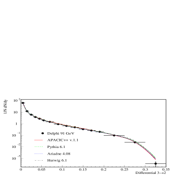
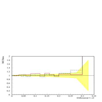
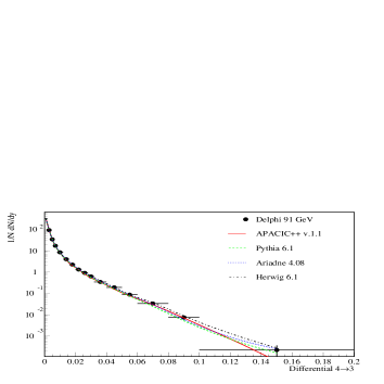
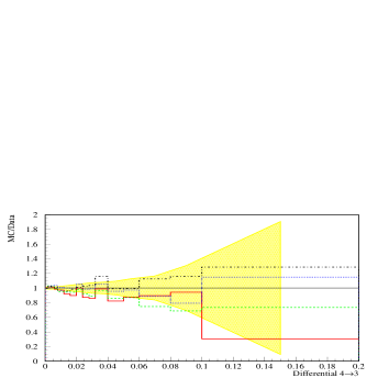
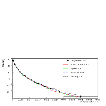
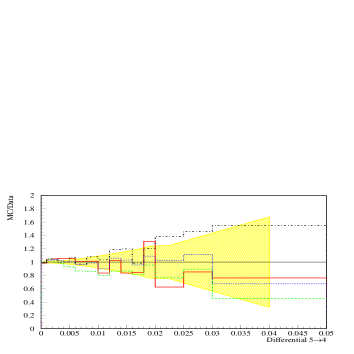
Figure 8: Differential $3\to 2$, $4\to 3$, and $5\to 4$ jet rates in the Durham algorithm at the $Z$–pole. DELPHI data (points) are compared to results (curves) of parton shower Monte Carlo generators. The shaded regions denote the size of the experimental errors.

Integrated jet rates taken at a c.m. energy of 189 GeV, defined here by the Cambridge algorithm [28], are displayed in Fig. 9. They demonstrate that APACIC++ extrapolates correctly to higher energies with all parameters fixed at the $Z$–pole.

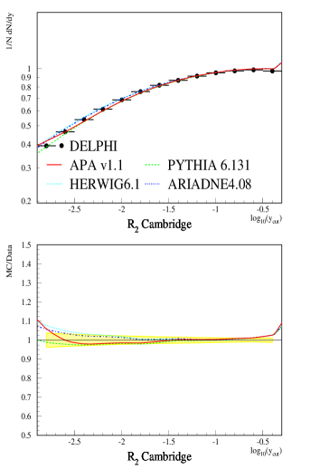
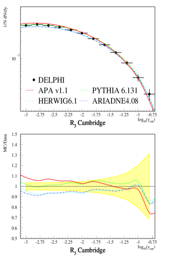
Figure 9: Integrated 2– and 3–jet rates defined by the Cambridge algorithm at ${\sqrt{s}}=189$ GeV. Note that the jet rates predicted by APACIC++ are in good agreement with the experimental ones in the regime of the matrix elements, i.e. to the right of $\log_{10}y_{\mbox{\scriptsize ini}}=-2.4$

To show that the approach outlined above does indeed reproduce not only the correct number of jets but also the overall shape of the events, we display some event shapes taken at the $Z$–pole (Fig. 10).

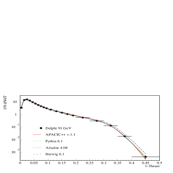
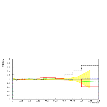
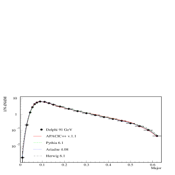
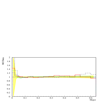
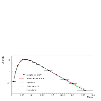
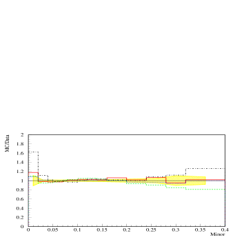
Figure 10: Some event shape (thrust, major and minor) distributions at the $Z$–pole.

In Fig. 11 we depict some momentum spectra. Here, all the event generators tend to underestimate the high-momentum regions. Given the fact that the overall shapes of the events tend to be reproduced fairly well by the generators, one is tempted to conclude that this reflects a lack of particle multiplicity in the high-momentum regions.

However, it should be stressed that the error bands in the right-hand plots consists of experimental errors – statistical and systematical – only. Monte–Carlo errors of the event generators are not included. To give some idea of the relative size of these errors, the numbers of events for the plots at 91 GeV are listed in Table 1.

DELPHI	Ariadne	Herwig	Pythia	APACIC++
350000	2000000	250000	2000000	500000

Table 1: Number of events used to generate the plots.

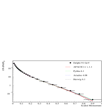
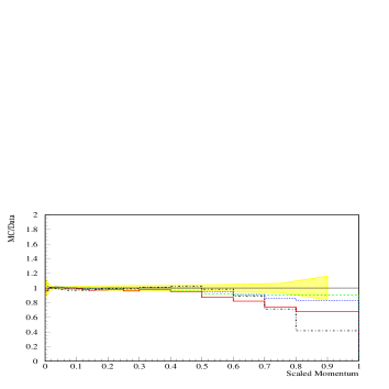
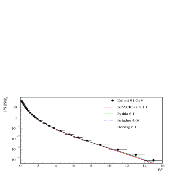
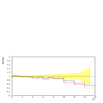
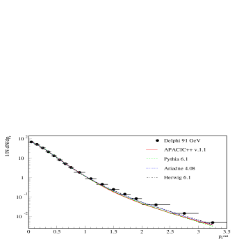
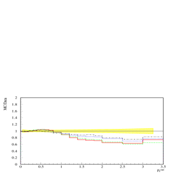
Figure 11: Scaled-momentum $(x=2p/{\sqrt{s}})$, $p_{t}^{\rm in}$ and $p_{t}^{\rm out}$ spectra at the $Z$–pole.

5 Comments/Conclusions

• Modified matrix elements plus vetoed parton showers, interfaced at some value $y_{\mbox{\scriptsize ini}}$ of the $k_{T}$-resolution parameter, provide a convenient way to describe simultaneously the hard multi-jet and jet fragmentation regions.

• The matrix element modifications are coupling-constant and Sudakov weights computed directly from the $k_{T}$-clustering sequence, which also serves to define the initial conditions for the parton showers.

• Dependence on $y_{\mbox{\scriptsize ini}}$ is cancelled to NLL accuracy by vetoing $y_{ij}>y_{\mbox{\scriptsize ini}}$ in the parton showers.

• This prescription avoids double-counting problems and missed phase-space regions.

• In principle one needs the tree–level matrix elements $|{\cal M}_{n,i}|^{2}$ for $y_{\mbox{\scriptsize cut}}>y_{\mbox{\scriptsize ini}}$ at all values of the parton multiplicity $n$. In practice, if we have $n\leq N$, then $y_{\mbox{\scriptsize ini}}$ must be chosen large enough for $R_{n>N}(y_{\mbox{\scriptsize ini}})$ to be negligible.

• An approximate version of this approach (with $N=5$) has been implemented in the event generator APACIC++ [20]. The results look promising: a rather good description of multi-jet observables can be achieved, and residual dependence on $y_{\mbox{\scriptsize ini}}$ is weak.

• It should be possible to extend this approach to lepton-hadron and hadron-hadron collisions. In particular, the procedure discussed in Sects. 2 and 3 can be extended to deep-inelastic lepton-hadron scattering by using the corresponding calculation of multi-jet rates performed in Ref. [29].

• Extension to NLO along the lines of Refs. [9, 10, 11, 12] may also be possible.

Taken together, the results show sufficient agreement with data to conclude that this approach to combining matrix elements and parton showers is successful and merges the benefits of both in a rather simple way. This approach can also be used to introduce corrections due to the finite mass of light (with respect to the c.m. energy) quarks, by combining the massive-quark matrix elements with the corresponding angular-ordered parton shower [30]. It has to be mentioned, however, that some significant deviations from the data remain. Therefore, additional improvements such as the inclusion of NLO matrix elements seem to be necessary to achieve better agreement.

References

- [1] A. S. Belyaev et al., hep-ph/0101232.
- [2] K. Sato, S. Tsuno, J. Fujimoto, T. Ishikawa, Y. Kurihara and S. Odaka, hep-ph/0104237.
- [3] M. L. Mangano, M. Moretti and R. Pittau, hep-ph/0108069.
- [4] E. Boos et al., hep-ph/0109068.
- [5] M. H. Seymour, Comput. Phys. Commun. 90 (1995) 95 [hep-ph/9410414], Nucl. Phys. B436 (1995) 443 [hep-ph/9410244].
- [6] J. Andre and T. Sjostrand, Phys. Rev. D57 (1998) 5767 [hep-ph/9708390]; G. Miu and T. Sjostrand, Phys. Lett. B449 (1999) 313 [hep-ph/9812455].
- [7] G. Corcella and M. H. Seymour, Phys. Lett. B442 (1998) 417 [hep-ph/9809451], Nucl. Phys. B565 (2000) 227 [hep-ph/9908388].
- [8] S. Mrenna, hep-ph/9902471.
- [9] C. Friberg and T. Sjostrand, hep-ph/9906316, in Proc. of Workshop on Monte Carlo Generators for HERA Physics, eds. T.A. Doyle, G. Grindhammer, G. Ingelman and H. Jung (DESY, Hamburg, 1999), p. 181.
- [10] J. Collins, JHEP 0005 (2000) 004 [hep-ph/0001040]; J. C. Collins and F. Hautmann, JHEP 0103 (2001) 016 [hep-ph/0009286]; Y. Chen, J. C. Collins and N. Tkachuk, JHEP 0106 (2001) 015 [hep-ph/0105291];
- [11] B. Potter, Phys. Rev. D 63, 114017 (2001) [hep-ph/0007172]; B. Potter and T. Schorner, Phys. Lett. B 517 (2001) 86 [hep-ph/0104261].
- [12] M. Dobbs, Phys. Rev. D 64, 034016 (2001) [hep-ph/0103174].
- [13] Y.L. Dokshitzer, in Workshop on Jet Studies at LEP and HERA, Durham 1990, see J. Phys. G17 (1991) 1572 ff.
- [14] S. Catani, Y. L. Dokshitzer, M. Olsson, G. Turnock and B. R. Webber, Phys. Lett. B269 (1991) 432.
- [15] S. Catani, B. R. Webber and G. Marchesini, Nucl. Phys. B 349, 635 (1991).
- [16] B. I. Ermolaev and V. S. Fadin, JETP Lett. 33 (1981) 269 [Pisma Zh. Eksp. Teor. Fiz. 33 (1981) 285]; A. H. Mueller, Phys. Lett. B 104 (1981) 161.
- [17] R. K. Ellis, W. J. Stirling and B. R. Webber, QCD and collider physics, (Cambridge University Press, Cambridge, 1996) and references therein.
- [18] G. Marchesini and B. R. Webber, Nucl. Phys. B310 (1988) 461.
- [19] Y. L. Dokshitzer, S. I. Troian and V. A. Khoze, Sov. J. Nucl. Phys. 47 (1988) 881 [Yad. Fiz. 47 (1988) 1384]; S. Catani, B. R. Webber, Y. L. Dokshitzer and F. Fiorani, Nucl. Phys. B 383 (1992) 419; P. Eden, G. Gustafson and V. Khoze, Eur. Phys. J. C 11 (1999) 345 [hep-ph/9904455].
- [20] F. Krauss, R. Kuhn and G. Soff, Acta Phys. Polon. B30 (1999) 3875 [hep-ph/9909572]; R. Kuhn, F. Krauss, B. Ivanyi and G. Soff, Comput. Phys. Commun. 134 (2001) 223 [hep-ph/0004270].
- [21] U. Flagmeyer, K. Hamacher, R. Kuhn, and F. Krauss, in preparation.
- [22] G. Marchesini, B. R. Webber, G. Abbiendi, I. G. Knowles, M. H. Seymour and L. Stanco, Comput. Phys. Commun. 67 (1992) 465; G. Corcella, I.G. Knowles, G. Marchesini, S. Moretti, K. Odagiri, P. Richardson, M.H. Seymour and B.R. Webber, JHEP 0101, 010 (2001) [hep-ph/0011363]; hep-ph/0107071.
- [23] T. Sjostrand, P. Eden, C. Friberg, L. Lonnblad, G. Miu, S. Mrenna and E. Norrbin, Comput. Phys. Commun. 135, 238 (2001) [hep-ph/0010017].
- [24] L. Lonnblad, Comput. Phys. Commun. 71 (1992) 15.
- [25] Maria Jose Mezquita Costa, private communications.
- [26] U. Flagmeyer, Masters–thesis (in German), 1996, WUD 96-25.
- [27] DELPHI collaboration, Z. Phys. C73 (1996) 11; M. Weierstall, PhD–thesis (in German), 1995, Bergische Univ.-GH Wuppertal, WU B DIS 95-11.
- [28] Y. L. Dokshitzer, G. D. Leder, S. Moretti and B. R. Webber, JHEP 9708 (1997) 001 [hep-ph/9707323].
- [29] S. Catani, Y. L. Dokshitzer and B. R. Webber, Phys. Lett. B285 (1992) 291.
- [30] G. Marchesini and B. R. Webber, Nucl. Phys. B330 (1990) 261.