CERN-TH/2001-254

hep-ph/0109230

Particle production from symmetry breaking
after inflation and leptogenesis

Juan García-Bellido  and  Ester Ruiz Morales

Theory Division, CERN, CH-1211 Genève 23, Switzerland

Recent studies suggest that the process of symmetry breaking after inflation typically occurs very fast, within a single oscillation of the symmetry-breaking field, due to the spinodal growth of its long-wave modes, otherwise known as ‘tachyonic preheating’. We show how this sudden transition from the false to the true vacuum can induce a significant production of particles, bosons and fermions, coupled to the symmetry-breaking field. We find that this new mechanism of particle production in the early Universe may have interesting consequences for the origin of supermassive dark matter and the generation of the observed baryon asymmetry through leptogenesis.

PACS numbers: 04.62.+v, 11.30.Qc, 11.15.Ex., 98.80.Cq

Keywords: Early Universe Cosmology, Particle Production, Dark Matter, Leptogenesis.

1 Introduction

Spontaneous symmetry breaking (SSB) is one of the basic ingredients of modern theories of elementary particles. It is usually assumed that SSB in Grand Unified and Electroweak theories took place in the early Universe through a thermal phase transition. However, it is also possible that some of these symmetries were broken at the end of a period of inflation [1], when the Universe had zero temperature and the negative mass term for the Higgs field appeared suddenly, i.e. in a time scale much shorter than the time required for SSB to occur. In this case, as was recently shown in Refs. [2], the process of symmetry breaking is extremely fast. The exponential growth of the Higgs quantum fluctuations is so efficient that SSB is typically completed within a single oscillation, while the field rolls down towards the minimum of its effective potential. This process, known as tachyonic preheating, leads to an almost instant conversion of the initial vacuum energy into classical waves of the scalar fields, in contrast with the process of ‘parametric preheating’, in which the inflaton field performs many oscillations before reheating the Universe [3].

In this letter we describe how this sudden transition from the false to the true vacuum can induce the non-adiabatic production of particles coupled to the Higgs. We also studied the consequences that this new process may have on the generation of the dark matter and the baryon asymmetry via leptogenesis. The phenomenon of particle production from symmetry breaking is analogous to the Schwinger mechanism [4], where the role of the external electric field pulse is played here by the time-dependent expectation value of the Higgs field. It is also similar to the well known process of particle production by a time-dependent gravitational background [5], responsible for the observed anisotropies of the microwave background, as well as for Hawking radiation [6]. The difference with respect to the standard mechanism of gravitational particle production in an expanding Universe is that, in our case, quantum excitations of fields coupled to the Higgs are produced due to the sharp change in their masses during the process of symmetry breaking, instead of due to the quick growth of the scale factor.

We will consider here a simplified model of SSB in which the Higgs instantly acquires a negative mass-squared term [2]. This ‘quench’ approximation corresponds to the limiting case of a hybrid inflation model [7] satisfying the so-called ‘waterfall’ condition. We therefore assume that the complex symmetry breaking field $\phi$ starts in the false vacuum at the top of its potential $V(\phi)=\lambda(|\phi|^{2}-v^{2})^{2}/4$, with zero mean, $\langle\phi\rangle=0$, and initial conditions given by vacuum quantum fluctuations. We will study the production of other fields, scalars $\chi$ and fermions $\psi$, coupled to the Higgs with the usual scalar $g^{2}|\phi|^{2}\chi^{2}$ and Yukawa $\,h\phi\bar{\psi}\psi\,$ interactions. As we will show later, the backreaction of the produced $\chi$ and $\psi$ modes on the evolution of the Higgs expectation value (vev) is negligible for the small $g$ and $h$ couplings we are considering, so that we can solve first the process of symmetry breaking, and then take the resulting evolution of the Higgs as a background field that induces particle production.

2 Symmetry Breaking

The dynamics of symmetry breaking has been studied in detail in Refs. [2]. Here we only summarise the main results needed for our analysis. At the initial stages of SSB, when re-scattering effects are still unimportant, the Higgs modes follow the linear equation $\ddot{\phi}_{k}+(k^{2}-m^{2})\,\phi_{k}=0$, where $m^{2}=\lambda\,v^{2}$. With vacuum initial conditions, $\phi_{k}(0)=1/\sqrt{2k},\ \dot{\phi}_{k}(0)=-ik\,\phi_{k}(0)$, all long-wavelength modes within the horizon ($H<k<m$) grow exponentially, $\phi_{k}(t)=\phi_{k}(0)\exp(t\sqrt{m^{2}-k^{2}})$, while modes with $k>m$ oscillate with constant amplitude. The exponential growth continues until the long-wave modes reach a value for which the effective Higgs mass becomes positive, i.e. when $\langle|\phi|^{2}\rangle\geq v^{2}/\sqrt{3}$, and the symmetry is broken soon after.

We have chosen $n_{k}+{1\over 2}=|\phi^{*}_{k}(t)\dot{\phi}_{k}(t)|$ as a proper definition for the occupation numbers of the Higgs tachyonic modes [8]. This expression does not require an a priori definition of a mode frequency $\omega_{k}$, and matches smoothly the one used in [2] for positive frequencies. For the growing modes, we have occupation numbers

$$n_{k}+{1\over 2}={1\over 2}\Big{|}e^{t\sqrt{m^{2}-k^{2}}}\Big{|}^{2}\approx{1\over 2}\,e^{2mt}\,e^{-{k^{2}\over 2k_{*}^{2}}}\,,$$ (1)

that become exponentially large very quickly for the long wavelength modes, and drop abruptly for $k>k_{*}=m\,(2mt)^{-1/2}$, which gives a natural ultraviolet cutoff for the problem. Note that, while the dynamics conserves $\langle\phi\rangle=0$, the Higgs dispersion also grows exponentially

$$\langle|\phi|^{2}\rangle={m^{2}\over 8\pi^{2}}\int_{0}^{m}{dk^{2}\over m^{2}}\,e^{2t\sqrt{m^{2}-k^{2}}}={m^{2}\over 16\pi^{2}}\,{e^{2mt}(2mt-1)+1\over m^{2}t^{2}}\sim{m^{2}\over 16\pi^{2}}\,e^{2mt}\,,$$ (2)

where this expression has been regularised, as described below. The time it takes for the system to break the symmetry, i.e. when $\langle|\phi|^{2}(t_{*})\rangle\simeq v^{2}$, can be estimated as

$$m\,t_{*}\simeq{1\over 2}\log\Big{(}{32\pi^{2}\over\lambda}\Big{)}\,.$$ (3)

This time depends only logarithmically on the Higgs self-coupling constant $\lambda$. For typical values, $\lambda=10^{-3}$ and $v=10^{-4}M_{\rm P}$, the symmetry is broken within $mt_{*}\sim 6$, and the typical cut-off frequency becomes $k_{*}\sim m/3$. This means that, by that time, the occupation numbers of modes with $k<k_{*}$ is exponentially large,

$$n_{k}(t_{*})\approx{1\over 2}e^{2mt_{*}}\simeq{16\pi^{2}\over\lambda}\sim 2\times 10^{5}\,.$$ (4)

These large occupation numbers allow us to treat these modes as semiclassical waves and match the solutions of the linear equations with the fully non-linear numerical lattice simulations [9]. The non-linear dynamics is studied by solving the real time evolution equations of classical fields, using a modified version of the lattice simulation program LATTICEEASY of Felder and Tkachev [10]. We start with initial fluctuations described by a Gaussian random field with zero mean, $\langle\phi_{k}\rangle=0$, and regularised dispersion

$$\langle|\phi_{k}^{2}(t)|\rangle_{\rm reg}\equiv\langle|\phi_{k}^{2}(t)|\rangle-{1\over 2\omega_{k}}\,.$$ (5)

This prescription amounts to substituting quantum averages by ensemble averages and ensures that the physical masses and energies are not ultraviolet divergent. In Fig. 1, we show the result of the full non-linear evolution of the Higgs vev, and compare it with the approximate expression

$$\phi(t)\equiv\langle|\phi|^{2}(t)\rangle^{1/2}={v\over 2}\Big{(}1+\tanh{m(t-t_{*})\over 2}\Big{)}\,,$$ (6)

which ignores the strongly damped oscillations after symmetry breaking [2]. We have checked that these low-amplitude oscillations do not contribute to the non-adiabatic production of particles; i.e. parametric preheating is inefficient after symmetry breaking, a result anticipated in Ref. [11] for the case of hybrid inflation. Note also that we are using the Higgs vev averaged over the lattice as a homogeneous background field, while it is actually a sum of tachyonic modes with different frequencies. However, in analogy with the generation of anisotropies during inflation, what drives the growth of long-wave modes $k<k_{*}$ of particles coupled to the Higgs is the coarse-grained Higgs vev over scales $\sim k^{-1}$, which is practically the same as the average over the whole Hubble volume, thanks to the fact that all Higgs modes with $H^{-1}<k<k_{*}$ grow essentially at the same speed.

3 Particle Production

We can now calculate the production of bosons and fermions coupled to the Higgs using the formalism of quantum fields in strong backgrounds [12, 13]. The mode equations in terms of rescaled fields, $X_{k}(t)=a^{3/2}\chi_{k}$ and $\Psi(t)=a^{3/2}\psi$, are

$$\partial_{t}^{2}X_{k}+\Big{(}k^{2}+m^{2}_{\rm B}(t)a^{2}(t)\Big{)}X_{k} = 0\,,$$ (7)

$$\Big{(}i\gamma^{\mu}\partial_{\mu}-m_{\rm F}(t)a(t)\Big{)}\Psi = 0\,,$$ (8)

where both the mass $m(t)$ and the scale factor $a(t)$ depend on time. In hybrid inflation models for which the quench approximation is valid, the rate of expansion is typically much smaller than the masses involved, and we can take the scale factor to be constant ($a=1$) during SSB. We will only consider here the non-adiabatic production of particles due to the change of vacuum as it induces a sudden change in the inertia (masses) of bosons $m^{2}_{\rm B}(t)=g^{2}\langle|\phi|^{2}\rangle$ and fermions $m_{\rm F}(t)=h\langle|\phi|^{2}\rangle^{1/2}$, through the Higgs mechanism.

We have solved the mode equations (7) and (8) both numerically, using the lattice Higgs vev evolution, and within the approximation (6), for which one has analytical solutions in terms of Hypergeometric functions [12]. The number density of created particles, as seen by a future observer in the true vacuum, is then given by

$$n_{X}={g_{s}\over 2\pi^{2}a^{3}}\,\int\,dk\,k^{2}\,|\beta_{k}|^{2}\,,$$ (9)

where $X$ denotes either bosons or fermions; $\beta_{k}$ are the Bogoliubov coefficients that relate the in ($t\to-\infty$) and out ($t\to+\infty$) mode functions; $k$ is the comoving momentum, and we have summed over spin indices ($g_{s}=1$ for scalars, 2 for spinors). In the case of charged fields, $n_{X}$ gives the number of particles, equal to that of antiparticles (i.e. $g_{s}=2$ for complex scalars, 2 for Majorana fermions, 4 for Dirac fermions).

Let us consider first the production of bosons. The mode functions $X_{k}(t)$ of the scalar field are solutions of the oscillator equation (7) with time-dependent frequency $\omega_{k}^{2}=k^{2}+m_{B}^{2}$, and initial vacuum conditions, $X_{k}(0)=1/\sqrt{2\omega_{k}}$ and $X^{\prime}_{k}(0)=-i\omega_{k}X_{k}$. In this case, the Bogoliubov coefficient at $t\to\infty$ can be written as $n_{k}^{\rm B}=|\beta_{k}|^{2}=(|X^{\prime}_{k}|^{2}+\omega_{k}^{2}|X_{k}|^{2}-\omega_{k})/2\,\omega_{k}$. The exact solution of the bosonic equation,

$$X^{\prime\prime}_{k}+\left(\omega_{-}^{2}(k)+{\alpha^{2}\over 4}(1+\tanh\,x)^{2}\right)\,X_{k}=0\,,$$ (10)

with $x=m(t-t_{*})/2$, can be written in terms of Hypergeometric functions as [12]

$$X_{k}=C_{1}(k)\,e^{ikt}(1+e^{mt})^{\tau}\,F(a,b,c;-e^{mt})+C_{2}(k)\,e^{-ikt}(1+e^{mt})^{\tau}\,F(a^{*},b^{*},c^{*};-e^{mt})\,,$$ (11)

where $\tau$ is a solution of the equation $\tau(\tau-1)+\alpha^{2}=0$, and

$$a=\tau+i(\omega_{-}-\omega_{+})\,,\hskip 28.45274ptb=\tau+i(\omega_{-}+\omega_{+})\,,\hskip 28.45274ptc=1+2i\,\omega_{-}\,,$$ (12)

where $\omega_{\pm}$ are the in/out asymptotic frequencies, $\omega_{-}(k)=k$ and $\omega_{+}(k)=\sqrt{k^{2}+\alpha^{2}m^{2}}$, and $\alpha\equiv g/\sqrt{\lambda}$. These solutions match the initial conditions at the end of inflation, and can be analytically continued to $t\to\infty$, in order to compute the boson occupation number $n_{k}^{\rm B}=|\beta_{k}|^{2}$,

$$n_{k}^{\rm B}(\alpha)={\cosh[\pi\sqrt{4\alpha^{2}-1}]+\cosh[2\pi(\omega_{+}-\omega_{-})/m]\over\sinh[2\pi\omega_{-}/m]\,\sinh[2\pi\omega_{+}/m]}\,.$$ (13)

A similar analysis can be done in the case of fermions, where the first-order Dirac equation (8) for the two spinor components can be written as an oscillator equation with complex frequency, $X^{\prime\prime}_{k}+(k^{2}+m_{F}^{2}-im_{F}^{\prime})\,X_{k}=0$, see Ref. [12],

$$X^{\prime\prime}_{k}+\left(\omega_{-}^{2}(k)+{\alpha^{2}\over 4}(1+\tanh\,x)^{2}-{i\alpha\over 4}(1+\tanh^{2}\,x)\right)\,X_{k}=0\,.$$ (14)

Given the initial vacuum conditions, $X_{k}(0)=(1-m_{F}/\omega_{k})^{1/2}$ and $X^{\prime}_{k}(0)=-i\omega_{k}X_{k}$, we can write the solution as in Eq. (11), but with $\tau=-i\alpha$. The fermionic occupation number can then be written as $n_{k}^{\rm F}=|\beta_{k}|^{2}=(\omega_{k}-m_{F}-{\rm Im}X_{k}{X_{k}^{\prime}}^{*})/2\,\omega_{k}$. Substituting the $t\to\infty$ solutions of the fermionic equations we find

$$n_{k}^{\rm F}(\alpha)={\cosh[2\pi\alpha]-\cosh[2\pi(\omega_{+}-\omega_{-})/m]\over 2\sinh[2\pi\omega_{-}/m]\,\sinh[2\pi\omega_{+}/m]}\,,$$ (15)

with $\omega_{-}$ and $\omega_{+}$ the same as for bosons but with $\alpha\equiv h/\sqrt{\lambda}$.

The occupation numbers obtained numerically from Eqs. (7) and (8), using the full non-linear lattice solution for the Higgs vev, agree very well with the analytical formulae (13) and (15), see Fig. 2, except at large momenta, where there is a small contribution from resonant particle production due to the strongly damped Higgs oscillations.

We will now calculate the ratio of energy densities of the particles created at the end of symmetry breaking to the initial false vacuum energy density

$${\rho_{X}\over\rho_{0}}={2g_{s}\lambda\over\pi^{2}}\int\,d\kappa\,\kappa^{2}\,n_{\kappa}^{X}(\alpha)\,\omega_{+}(\kappa,\alpha),$$ (16)

where $\kappa=k/m$ and $\rho_{0}=m^{4}/4\lambda$. We can obtain a fit to the final energy density of bosons and fermions as

$$\rho_{\rm B}/\rho_{0} \simeq 2\times 10^{-3}\,g_{s}\lambda\,f(\alpha,1.3)\,,$$ (17)

$$\rho_{\rm F}/\rho_{0} \simeq 1.5\times 10^{-3}\,g_{s}\lambda\,f(\alpha,0.8)\,,$$ (18)

where the fitting function is $f(\alpha,\gamma)\equiv\sqrt{\alpha^{2}+\gamma^{2}}-\gamma$, and the coefficient $\alpha=g/\sqrt{\lambda}\,(h/\sqrt{\lambda})$ for bosons (fermions), has been fitted in the range $\alpha\in[0.01,10]$.

We can also write the number densities for bosons and fermions,

$$n_{\rm B}(\alpha) \simeq 1\times 10^{-3}g_{s}\,m^{3}\,f(\alpha,1.3)/\alpha\,,$$ (19)

$$n_{\rm F}(\alpha) \simeq 3.6\times 10^{-4}g_{s}\,m^{3}\,f(\alpha,0.8)/\alpha\,.$$ (20)

From these expression we see that the production of bosons and fermions from symmetry breaking is more efficient when the Higgs mass and thus $\lambda$ is large, driving a very steep growth of the vev towards the true vacuum. In the case of very large couplings $g^{2},h^{2}\gg\lambda$, the produced particles are non-relativistic, $\omega_{k}\approx m_{X}$, and their energy density is given by $\rho_{\rm X}=m_{\rm X}n_{\rm X}$. Although the energy density increases with the mass of the particles produced, their number density saturates for large $\alpha$ to a value proportional to $m^{3}$, and thus the number of particles produced cannot be made arbitrarily large by increasing $g$ and $h$ couplings. Furthermore, the physical momenta redshift as $k_{\rm phys}=k/a$ with the expansion of the Universe, and thus the number density of both relativistic and non-relativistic bosons or fermions decays as $n_{X}\sim a^{-3}$.

Note that, unless the couplings are unnaturally large, the fractional energy density in bosons and fermions is always small, so we do not expect an important backreaction on the evolution of the Higgs condensate as the symmetry is broken. Moreover, contrary to the case of Ref. [14], in which particles are produced long after symmetry breaking from non-linear rescattering, our mechanism of particle production from symmetry breaking gives an upper limit to the occupation numbers of bosons produced in the range $H<k<m$, even for arbitrarily large coupling $g$, which is of order $n_{k}\leq 1$. This prevents us from using LATTICEEASY to compute their energy density and backreaction.

We would like to explore now the cosmological consequences that this production of particles may have for the evolution of the Universe.

4 Leptogenesis

Leptogenesis from preheating was first proposed in Ref. [15] in the context of chaotic inflation, where the right-handed (RH) neutrinos were produced via parametric resonance through their coupling to the inflaton. Here we propose a novel scenario in which a large population of out-of-equilibrium RH neutrinos is produced in the process of symmetry breaking after hybrid inflation, via their coupling to the SSB field.

Let us suppose that the symmetry-breaking field responsible for the end of hybrid inflation, and undergoing tachyonic preheating, is in fact the Higgs field of a grand unified theory (GUT) with ($B-L$)-violating interactions, and that the same Higgs produces a significant population of right-handed Majorana neutrinos via the non-perturbative mechanism described above. These massive neutrinos decay (out of equilibrium) into leptons and standard model (SM) Higgses, generating a leptonic asymmetry [17] that later gets converted into the baryon asymmetry of the Universe via sphaleron transitions [18].

The Lagrangian terms relevant for leptogenesis are

$${\cal L}=-{1\over 2}\,h\,\bar{N}^{c}_{R}\,\phi\,N_{R}-h_{\nu}\,\bar{N}\,H\,l_{L}\,,$$ (21)

where the first term determines the masses of RH neutrinos through the GUT Higgs mechanism, $M_{R}=h\,\langle\phi\rangle=h\,v$, while the second term determines the lepton-violating decays of the RH neutrinos into SM Higgses $H$ and left-handed leptons $l_{L}$. Although both Yukawas $h$ and $h_{\nu}$ are actually 3x3 matrices, we will not consider here the complications of 3-generation neutrino masses and mixings, but will assume as usual [19] that only the lightest RH neutrino $N_{1}$, with mass $M_{1}$, is responsible for leptogenesis. For analogous reasons, the CP-violating asymmetry $\varepsilon$ in the decay of the RH neutrino, which also depends on the structure of neutrino masses and mixing, will be taken as a free parameter.

Assuming that the masses of the SM light neutrinos are generated by the see-saw mechanism [20], $m_{\nu_{i}}=(m_{D}m_{D}^{\dagger})_{ii}/M_{i}$, the decay rate of the lightest RH neutrino can be written in terms of $m_{\nu_{1}}$ and $M_{1}$ as

$$\Gamma_{N_{1}}={G_{F}\over 2\sqrt{2}\,\pi}\,m_{\nu_{1}}\,M_{1}^{2}=4.12\times 10^{6}\,h^{2}\,\left({v\over 10^{15}\,{\rm GeV}}\right)^{2}\left({m_{\nu_{1}}\over 10^{-9}\,{\rm eV}}\right)\,{\rm GeV}\,.$$ (22)

Under these assumptions, the model has 5 parameters: the vev of the GUT Higgs $v$, the Higgs self-coupling $\lambda$, the Yukawa coupling of the RH neutrino $h$, the mass of the light neutrino $m_{\nu_{1}}$, and the final reheating temperature $T_{\rm rh}$. We will now study the constraints that will determine the allowed range of parameters for a successful model of leptogenesis.

The first requirement is that the RH neutrinos produced at symmetry breaking decay out of equilibrium. To ensure this we impose two conditions: i) that the Higgses produced via tachyonic preheating do not reach thermal equilibrium before the RH neutrinos decay; and ii) that the Higgs-neutrino interaction rate is much smaller than the rate of expansion of the Universe, so that even if the Higgses thermalise, the RH neutrinos remain out of equilibrium.

In order to satisfy condition i), we require that the Higgs self-interaction rate at the time of symmetry breaking is smaller than the rate of expansion, $\Gamma_{\rm self}<H_{\rm SB}=(2\pi/3)^{1/2}\,m\,v/M_{\rm P}$, where

$$\Gamma_{\rm self}=\int\,{d^{3}k\over(2\pi)^{3}}\,\sigma_{\rm self}\,n_{k}^{\phi}(t_{*})\,{k\over m}={2\lambda m\over\pi\ln(32\pi^{2}/\lambda)}\,,$$ (23)

with $\sigma_{\rm self}={\lambda^{2}\over 8\pi k_{*}^{2}}$ and $n_{k}^{\phi}(t_{*})={16\pi^{2}\over\lambda}\,e^{-k^{2}/2k_{*}^{2}}$. Note that, once ensured at symmetry breaking, this condition is always satisfied since $n_{\phi}(t)\sim a^{-3}$ while $H\sim t^{-1}$. This condition constrains the Higgs self-coupling to be

$${\lambda\over\ln(32\pi^{2}/\lambda)}<\Big{(}{\pi^{3}\over 6}\Big{)}^{1/2}\,{v\over M_{\rm P}}\,.$$ (24)

Once chosen a GUT scale $v$, this constraint gives an upper bound on $\lambda$, and thus on the maximum number of RH neutrinos produced in this model. We will take $v=10^{15}$ GeV, and $\lambda=10^{-3}$, which satisfies the bound.

The second constraint ii) requires $\Gamma_{\rm int}<H_{\rm SB}$, where

$$\Gamma_{\rm int}=\int\,{d^{3}k\over(2\pi)^{3}}\,\sigma_{\rm int}\,n_{k}^{\phi}(1-n_{k}^{F})\,{k\over m}={h^{2}m\over\pi^{2}\ln^{2}(32\pi^{2}/\lambda)}\,,$$ (25)

with the Higgs-$N_{1}$ cross-section given by $\sigma_{\rm int}={h^{4}\over 16\pi^{2}M_{1}^{2}}$, and where we have neglected the fermion contribution $n_{k}^{F}\ll 1$. This gives

$${h\over\ln(32\pi^{2}/\lambda)}<\Big{(}{2\pi^{5}\over 3}\Big{)}^{1/4}\,\Big{(}{v\over M_{\rm P}}\Big{)}^{1/2}\,.$$ (26)

For the chosen parameters, we can satisfy this constraint as long as $h<0.5$. We will choose $h=0.01$, i.e. $M_{1}=10^{13}$ GeV. With these values of the parameters, the number density (20) and fractional energy density (18) of RH neutrinos at symmetry breaking becomes $n_{N_{1}}\simeq 1.4\times 10^{-4}\,m^{3}$ and $\rho_{N_{1}}/\rho_{0}\simeq 7.4\times 10^{-6}$.

We will now study the constraints associated with the time of decay of the RH neutrinos, $t_{1}=\Gamma_{N_{1}}^{-1}$. Since $v$, $\lambda$ and $h$ have been determined by the previous constraints, these new conditions will give an allowed range for $m_{\nu_{1}}$. First of all, the $N_{1}$ lifetime should be greater than the time of symmetry breaking, $t_{1}\geq t_{*}$, with $t_{*}$ given in (3). For our parameters, we should satisfy

$$m_{\nu_{1}}<0.5\ {\rm eV}\left({10^{15}\,{\rm GeV}\over v}\right)\,{\sqrt{\lambda}\over h^{2}\ln(32\pi^{2}/\lambda)}=12\ {\rm eV}\,.$$ (27)

We also have to ensure that the annihilation rate of $N_{1}$ into Higgses, $\Gamma_{\rm ann}=n_{N_{1}}\,\sigma_{\rm ann}$, with annihilation cross-section $\sigma_{\rm ann}=h^{4}/16\pi^{2}M_{1}^{2}$, is smaller than the decay rate, $\Gamma_{\rm ann}<\Gamma_{N_{1}}$, otherwise no RH neutrinos would be left to produce the lepton asymmetry. This imposes the constraint

$$m_{\nu_{1}}>1.1\times 10^{-6}\ {\rm eV}\,{\lambda^{2}\over h}\,f(h/\sqrt{\lambda},0.8)\,\left({10^{15}\,{\rm GeV}\over v}\right)=7\times 10^{-12}\ {\rm eV}\,,$$ (28)

which gives, together with (27), a wide range of allowed $m_{\nu_{1}}$ values.

Finally, we want our RH neutrinos to decay before the Universe reheats via the decay of the Higgs, $\Gamma_{N_{1}}>\Gamma_{\phi}=H(t_{\rm rh})$. This implies a bound on the reheating temperature, $T_{\rm rh}\sim 0.12\sqrt{\Gamma_{\phi}M_{\rm P}}$ [21],

$$T_{\rm rh}<2\times 10^{-3}\,M_{1}\,\left({m_{\nu_{1}}\over 10^{-9}\,{\rm eV}}\right)^{1/2}\,.$$ (29)

For $M_{1}=10^{13}$ GeV, and chosing the mass of the light neutrino to be $m_{\nu_{1}}=10^{-9}$ eV, we find that the reheating temperature should satisfy $T_{\rm rh}<2\times 10^{10}$ GeV, which is compatible with the bounds coming from gravitino production.

Now we should estimate the effective temperature of the decay products of the RH neutrinos $\tilde{T}_{1}$, assuming that their energy density at the time of decay $t_{1}$ is converted into a thermal bath $\rho_{N_{1}}(t_{1})={\pi^{2}\over 30}g_{*}\tilde{T}_{1}^{4}$. The neutrino energy density at $t_{1}$ can be calculated from its value at symmetry breaking as

$$\rho_{N_{1}}(t_{1})=\left({\rho_{N_{1}}\over\rho_{\phi}}\right)_{\rm SB}\left({H_{\rm SB}\over\Gamma_{N_{1}}}\right)^{1/2}\rho_{\phi}(t_{1}),$$ (30)

taking into account that, from $t_{\rm SB}$ until $t_{1}$, the RH neutrinos are non-relativistic and thus their energy density decays like matter, $\rho_{F}\sim a^{-3}$, while the energy density in Higgs particles is dominated by the gradient and kinetic terms, with a radiation equation of state, $\rho_{\phi}\sim a^{-4}$. This gives the extra factor $a(t_{1})/a(t_{\rm SB})$ in (30) coming from the expansion of the Universe. Since at $t_{1}$ the energy density is dominated by the inflaton, we have $\rho_{\phi}(t_{1})=3M_{\rm P}^{2}\Gamma_{N_{1}}^{2}/8\pi$. For our parameters, we find

$$\tilde{T}_{1}=2\times 10^{12}\ {\rm GeV}\,h^{3/2}\,\lambda^{5/16}\,f^{1/4}(h/\sqrt{\lambda},0.8)\,\left(v\over{10^{15}\,{\rm GeV}}\right)=4\times 10^{9}\ {\rm GeV}\,,$$ (31)

which does not constitute a problem with gravitino production.

A final concern is that the lepton-number-violating processes among the particles in this thermal bath are always out of equilibrium, so that they do not wash out the lepton asymmetry produced, $\Gamma_{\Delta L=2}={4\over\pi^{3}}\tilde{T}_{1}^{3}\,G_{\rm F}^{2}\,\sum m_{\nu_{i}}^{2}<H(\tilde{T}_{1})$. We have included here the possible channels of lepton-number violating interactions mediated by the heavy RH neutrinos $N_{2}$ and $N_{3}$. This bound gives

$$\tilde{T}_{1}<3.3\times 10^{13}\ {\rm GeV}\,\left({3\times 10^{-3}\,{\rm eV}^{2}\over\sum m_{\nu_{i}}^{2}}\right)\,,$$ (32)

which is easily satisfied, see Eq. (31), for the range of light neutrino masses consistent with neutrino oscillations [22].

We may now ask how efficient is this mechanism for producing the required amount of baryons in the Universe, $n_{\rm B}/s=(4-9)\times 10^{-11}$, where $s$ is the entropy density, and we use the fact that this ratio remains constant since reheating.

The baryon asymmetry is produced via sphaleron transitions that violate $(B+L)$ and convert a lepton asymmetry into a baryon asymmetry, $n_{\rm B}=(28/79)n_{\rm L}$ [18]. The entropy density at reheating can be computed in terms of the energy density, $s=(4/3)\rho_{\phi}/T_{\rm rh}$, and can be estimated as

$$\left.{n_{\rm B}\over s}\right|_{0} = \left.{28\over 79}\,{n_{\rm L}\over s}\right|_{\rm rh}=\left.{28\over 79}\,{3T_{\rm rh}\over 4}\,{n_{\rm L}\over\rho_{\phi}}\right|_{\rm rh}={28\over 79}\,{3n_{\rm L}\over 4n_{N_{1}}}\,T_{\rm rh}\,\left.{n_{N_{1}}\over\rho_{\phi}}\right|_{\rm SB}\left({\rho_{0}\over\rho_{\rm rh}}\right)^{1/4}$$ (33)

$$= 2.2\times 10^{-4}\,\varepsilon\,{\lambda^{5/4}\over h}\,f(h/\sqrt{\lambda},0.8)\,,$$

where we have assumed that the lepton number density is directly related to the number density of RH neutrinos via $n_{\rm L}=\varepsilon\,n_{N_{1}}$. For the values of the parameters we have chosen, the baryon asymmetry becomes $n_{\rm B}/s=2.3\times 10^{-7}\,\varepsilon$, which requires a relatively large leptonic asymmetry $\varepsilon=3.4\times 10^{-4}$, that could be obtained in realistic neutrino models with large mixing angles. However, significantly smaller values of $\varepsilon$ can still be accommodated in this scenario since the values we chose for $h$ and $\lambda$ were very conservative. If we keep the GUT vev at $10^{15}$ GeV, we can still increase the production of RH neutrinos by taking the maximum values of the couplings allowed by the bounds (24) and (26), $h=0.5$ and $\lambda=3\times 10^{-3}$, which gives $\varepsilon\geq 7\times 10^{-5}$ for agreement with the observed baryon asymmetry of the Universe. Moreover, the value of $\lambda$ can be chosen greater than the bound (24) if we accept that the Higgses thermalise (before decaying) soon after symmetry breaking, while keeping $h$ small (26), so that the RH neutrinos remain out of equilibrium before decaying.

We can also choose a larger vev for the GUT Higgs, e.g. $v=10^{16}$ GeV, thus allowing a larger RH neutrino production. This vev value would be compatible with all the bounds, and permits a maximum value for $\lambda=0.02$ and $h=1.15$, which gives $n_{\rm B}/s=1.12\times 10^{-5}\,\varepsilon$. This corresponds to values of the leptonic asymmetry as small as $\varepsilon=7\times 10^{-6}$, to be in agreement with the observed baryon asymmetry of the Universe. Smaller values of $\varepsilon$ would be difficult to accommodate in our scenario.

We conclude that our scenario can generate a successful leptogenesis for a wide range of model parameters, although in order to go beyond our estimates, we would need more information on the structure of neutrino masses and mixings.

5 Other relics, dark matter and cosmic rays

This out-of-equilibrium production of particles during SSB may have other interesting cosmological consequences. For instance, this mechanism may be responsible for the non-thermal production of superheavy dark matter (SDM) [23]. Consider the following scenario: a GUT scale symmetry breaking at the end of a period of hybrid inflation, where the SB field may generate via the mechanism described above, a large population of particles out of equilibrium, which may either decay into stable relics, or be stable themselves. Such a heavy relic will eventually dominate the energy density of the Universe and constitute today the cold dark matter component, $\Omega_{\rm cdm}h^{2}=0.14\pm 0.04$, $95\%$ c.l. [24], where $h=0.72\pm 0.07$ is the present Hubble rate in units of 100 km/s/Mpc.

Assuming that the relic dark matter particles were produced soon after symmetry breaking and that the Universe reheated at a temperature $T_{\rm rh}$, we can estimate the fraction of energy in these non-relativistic particles today as

$${\Omega_{X}h^{2}\over\Omega_{\gamma}h^{2}}\simeq{\rho_{X}\over\rho_{\rm SB}}\,{T_{\rm rh}\over T_{0}}\,,$$ (34)

where $\rho_{X}=r\,\rho_{Y}$ if the relic particles come from the decay, with branching ratio $r$, of species $Y$ produced at symmetry breaking. Note that in the simplest case in which species $X$ couple directly to the GUT Higgs, $r=1$, but in general we expect $r\ll 1$. Substituting the present temperature of the Universe, $T_{0}=2.73$ K $=2.4\times 10^{-13}$ GeV, we have

$${\rho_{X}\over\rho_{\rm SB}}=2\times 10^{-19}\,\left({10^{10}\,{\rm GeV}\over T_{\rm rh}}\right)\,.$$ (35)

Using expressions (17) and (18), we see that in the limit of small couplings, $\rho_{X}/\rho_{\rm SB}\simeq 2\times 10^{-3}\,g_{X}^{2}$, where $g_{X}$ is the coupling to the Higgs, which gives it a mass $M_{X}=g_{X}10^{15}$ GeV. In order that the X-particle relics be the cold dark matter today, we require

$$M_{X}=10^{7}\,{\rm GeV}\,\left({10^{10}\,{\rm GeV}\over T_{\rm rh}}\right)^{1/2}\,.$$ (36)

For a reheating temperature as high as $T_{\rm rh}=10^{10}$ GeV, the mass of the particle becomes $M_{X}=10^{7}$ GeV $<T_{\rm rh}$, and is thus non-relativistic at symmetry breaking. In this case, its energy density decays like radiation until its mass is of order the temperature of the Universe, so we should substitute $T_{\rm rh}\to M_{X}$ in Eqs. (34) and (35). Therefore, Eq. (36) determines $M_{X}=10^{8}$ GeV, a very natural candidate for SDM.

However, we must make sure that the SDM relics remain out of equilibrium since their production, otherwise their thermal population would be completely unacceptable today. For this we must ensure that their annihilation rate is always much smaller than the expansion rate, $\Gamma_{\rm ann}=n_{X}(T_{\rm rh})\,\sigma_{\rm ann}|v|\ll H(T_{\rm rh})$, where the annihilation crossection is $\sigma_{\rm ann}=g_{X}^{4}/(16\pi^{2}M_{X}^{2})$. Using expressions (19) and (20) in the small coupling limit, $n_{X}=4.8\times 10^{-4}\,\lambda\,g_{X}^{-2}\,M_{X}^{3}$, we get, for $\lambda=10^{-3}$,

$$\Gamma_{\rm ann}=3\times 10^{6}\,{\rm GeV}\,g_{X}^{3}\ \ll\ 200\,{\rm GeV}\,\left({T_{\rm rh}\over 10^{10}\,{\rm GeV}}\right)^{2}=H(T_{\rm rh})\,.$$ (37)

It is clear that for the case above, with $g_{X}=10^{-7}$, we are always safe.

Alternatively, we may consider the production of X-particles from the decay, with very small branching ratio $r\sim 10^{-10}$, of very heavy Y-particles produced at SSB, with e.g. $M_{Y}=10^{12}$ GeV and $M_{X}\sim 10^{11}$ GeV. For this value of the coupling, $g_{Y}=10^{-3}$, the Y-particles remain always out of equilibrium, see (37), while their energy density at symmetry breaking is given by $\rho_{Y}/\rho_{\rm SB}=2\times 10^{-9}$, giving rise to a dark matter relic X which is compatible with present bounds.

Moreover, a very interesting consequence of this population of extremely weakly coupled heavy relics produced at GUT symmetry breaking is that they may constitute the origin of the ultra high energy cosmic rays [25]. In the case the X-particles are metastable, with lifetime of the order of the age of the Universe, their mass $M_{X}\sim 10^{11}$ GeV $=10^{20}$ eV may be converted into extremely energetic particles that reach Earth today and whose nature could in the near future be studied by the Pierre Auger project, the high-resolution fly’s eye, and the Japanese telescope array project [25].

6 Conclusions

In this letter we have shown that the exponential growth of the Higgs vev towards its true vacuum at the end of a period of hybrid inflation, known as tachyonic preheating, can induce a significant production of particles, both bosons and fermions coupled to the Higgs. This new mechanism of particle production in the early Universe could be responsible for generating the observed baryon asymmetry via leptogenesis, as well as the present dark matter of the Universe.

We have proposed a novel scenario for leptogenesis, in which a large population of out-of-equilibrium RH neutrinos is generated in the process of symmetry breaking after hybrid inflation, assuming that the symmetry breaking field is actually the Higgs field of a grand unified theory (GUT) with ($B-L$)-violating interactions. We have shown that this is indeed an attractive leptogenesis scenario, since it can explain the observed baryon asymmetry for a wide range of model parameters.

In the case that stable relics are produced out-of-equilibrium from the decay products of the GUT Higgs, it is possible that they may constitute today the observed cold dark matter. These particles may have masses as large as $10^{13}$ GeV, and could be responsible (if metastable) for the observed flux of ultra high energy cosmic rays.

Figure Captions

Figure 1. The time evolution of the vacuum expectation value $\langle\phi^{2}(t)\rangle^{1/2}/v$, as compared with the approximate solution (6) with $mt_{*}=8$. We have used a lattice of size N=128 and length L=100$\pi$, which gives $k_{\rm min}=2H=0.02m$ and $k_{\rm max}=2.22m$. We also show the evolution of the number density, $n_{\rm B}(t)$, in units of $100\,m^{-3}$, for bosonic particles coupled to the Higgs with $g=0.5$.

Figure 2. The spectrum of occupation numbers for both bosons and fermions in the (asymptotic) true vacuum, using the lattice results for the Higgs vev, as compared with the analytical formulae (13) and (15). The parameters chosen here are $\lambda=0.01$, $g=0.5$ and $h=0.5$. The tiny peaks at large momenta correspond to small resonances due to the strongly damped Higgs oscillations after SSB.

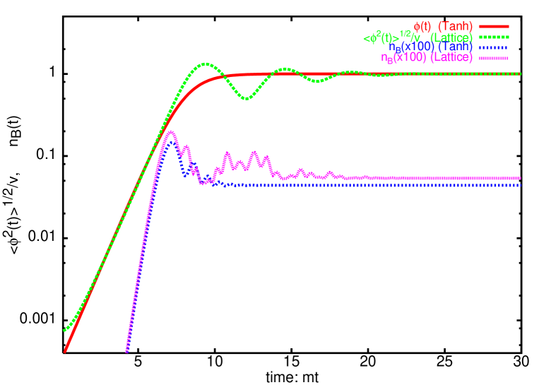
Figure 1:

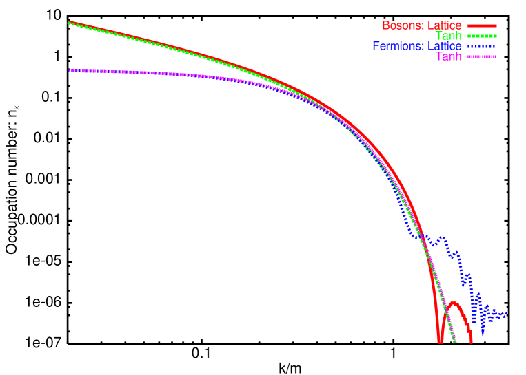
Figure 2:

References

- [1] J. García-Bellido, D. Grigoriev, A. Kusenko and M. Shaposhnikov, Phys. Rev. D 60 (1999) 123504 [hep-ph/9902449].
-
[2]
G. Felder, J. García-Bellido, P. B. Greene,
L. Kofman, A. Linde and I.I. Tkachev, Phys. Rev. Lett. 87
(2001) 011601 [hep-ph/0012142];
G. Felder, L. Kofman and A. Linde, Phys. Rev. D 64 (2001) 123517 [hep-th/0106179]. - [3] L. Kofman, A. Linde and A. A. Starobinsky, Phys. Rev. Lett. 73 (1994) 3195 [hep-th/9405187]; Phys. Rev. D 56 (1997) 3258 [hep-ph/9704452].
- [4] J. Schwinger, Phys. Rev. 82 (1951) 664.
-
[5]
L. Parker, Phys. Rev. 183 (1969) 1057;
A.A. Grib and S.G. Mamaev, Sov. J. Nucl. Phys. 10 (1970) 722;
Ya. B. Zel’dovich and A.A. Starobinskii, Sov. Phys. JETP 34 (1972) 1159. - [6] S.W. Hawking, Nature 248 (1974) 30.
- [7] A.D. Linde, Phys. Lett. B259 (1991) 38; Phys. Rev. D 49 (1994) 748 [astro-ph/9307002].
- [8] M. Salle, J. Smit, J.C. Vink, hep-ph/0112057.
-
[9]
S.Yu. Khlebnikov and I.I. Tkachev, Phys. Rev. Lett.
77 (1996) 219 [hep-ph/9603378];
79 (1997) 1607 [hep-ph/9610477];
T. Prokopec and T.G. Roos, Phys. Rev. D 55 (1997) 3768 [hep-ph/9610400]. - [10] G. Felder and I.I Tkachev, “LATTICEEASY: A program for lattice simulations of scalar fields in an expanding Universe”, hep-ph/0011159.
- [11] J. García-Bellido and A. D. Linde, Phys. Rev. D 57 (1998) 6075 [hep-ph/9711360].
- [12] A. A. Grib, S. G. Mamayev, and V. M. Mostepanenko, Vacuum quantum effects in strong fields, Friedmann Laboratory, St. Petersburg, 1994.
- [13] N.D. Birrel and P.C.W. Davies, Quantum fields in curved space, Cambridge University Press, Cambridge 1982.
- [14] G. Felder and L. Kofman, Phys. Rev. D 63 (2001) 103503 [hep-ph/0011160].
- [15] G.F. Giudice, M. Peloso, A. Riotto and I. Tkachev, JHEP 9908 (1999) 014 [hep-ph/9905242].
-
[16]
P. B. Greene and L. Kofman,
Phys. Lett. B 448 (1999) 6 [hep-ph/9807339];
J. García-Bellido, S. Mollerach and E. Roulet, JHEP 0002 (2000) 034 [hep-ph/0002076]. - [17] M. Fukugita and T. Yanagida, Phys. Lett. B 174 (1986) 45.
- [18] S.Yu. Khlebnikov and M.E. Shaposhnikov, Nucl. Phys. B 308 (1988) 885.
- [19] W. Buchmüller and M. Plümacher, Phys. Rep. 320 (1999) 329 [hep-ph/9904310].
- [20] M. Gell-Mann, P. Ramond and R. Slansky, in Supergravity (North Holland, Amsterdam 1979); T. Yanagida, in Unified Theory and Baryon Number of the Universe (KEK, Japan 1979).
- [21] A. D. Linde, Particle physics and inflationary cosmology, Harwood Academic Press, New York, 1990.
- [22] J. N. Bahcall, M. C. González-García and C. Peña-Garay, JHEP 0108 (2001) 014 [hep-ph/0106258].
- [23] D.J.H. Chung, E.W. Kolb and A. Riotto, Phys. Rev. Lett. 81 (1998) 4048 [hep-ph/9805473]; Phys. Rev. D 59 (1999) 023501 [hep-ph/9802238].
- [24] A. Melchiorri and J. Silk, astro-ph/0203200.
- [25] V. Kuzmin and I. Tkachev, Phys. Rev. D 59 (1999) 123006 [hep-ph/9809547]; Phys. Rept. 320 (1999) 199 [hep-ph/9903542]