Calculation of two-loop virtual corrections to $b\!\rightarrow\!s\ell^{+}\ell^{-}$
in the standard model

Abstract

We present in detail the calculation of the virtual ${\mathcal{O}}(\alpha_{s})$ corrections to the inclusive semi-leptonic rare decay $b\rightarrow s\ell^{+}\ell^{-}$. We also include those ${\mathcal{O}}(\alpha_{s})$ bremsstrahlung contributions which cancel the infrared and mass singularities showing up in the virtual corrections. In order to avoid large resonant contributions, we restrict the invariant mass squared $s$ of the lepton pair to the range $0.05\leq s/m_{b}^{2}\leq 0.25$. The analytic results are represented as expansions in the small parameters $\hat{s}=s/m_{b}^{2}$, $z=m_{c}^{2}/m_{b}^{2}$ and $s/(4m_{c}^{2})$. The new contributions drastically reduce the renormalization scale dependence of the decay spectrum. For the corresponding branching ratio (restricted to the above $\hat{s}$-range) the renormalization scale uncertainty gets reduced from $\sim\pm 13\%$ to $\sim\pm 6.5\%$.

I Introduction

Rare $B$-decays are an extremely helpful tool for examining the standard model (SM) and searching for new physics. Within the SM, they provide checks on the one-loop structure of the theory and allow one to retrieve information on the Cabibbo-Kobayashi-Maskawa (CKM) matrix elements $V_{ts}$ and $V_{td}$, which cannot be measured directly.

The first measurement of the exclusive rare decay $B\rightarrow K^{*}\gamma$ was obtained in 1992 by the CLEO collaboration [1]. Somewhat later, also the inclusive transition $B\rightarrow X_{s}\gamma$ was observed by the same collaboration [2]. Although challenging for the experimentalists, the inclusive decays are clean from the theoretical point of view, as they are well approximated by the underlying partonic transitions, up to small and calculable power corrections which start at ${\mathcal{O}}(\Lambda_{\rm{QCD}}^{2}/m_{b}^{2})$ [3, 4].

The measured photon energy spectrum [5] and the branching ratio for the decay $B\rightarrow X_{s}\gamma$ [2, 6, 7] are in good agreement with the next-to-leading logarithmic (NLL) standard model predictions (see e.g. [8, 9, 10, 11, 12, 13, 14]). Consequently, the decay $B\rightarrow X_{s}\gamma$ places stringent constraints on the extensions of the SM, such as two-Higgs doublet models [10, 15, 16], supersymmetric models [17, 18, 19, 20, 21, 22], etc.

$B\rightarrow X_{s}\ell^{+}\ell^{-}$ is another interesting rare decay mode which has been extensively considered in the literature in the framework of the SM and its extensions (see e.g [23, 24, 25, 26, 27, 28]). This decay has not been observed so far, but it is expected to be measured at the operating $B$-factories after a few years of data taking (for upper limits on its branching ratio we refer to [29, 30]). The measurement of various kinematical distributions of the decay $B\rightarrow X_{s}\ell^{+}\ell^{-}$, combined with improved data on $B\rightarrow X_{s}\gamma$, will tighten the constraints on the extensions of the SM or perhaps even reveal some deviations.

The main problem of the theoretical description of $B\rightarrow X_{s}\ell^{+}\ell^{-}$ is due to the long-distance contributions from $\bar{c}c$ resonant states. When the invariant mass $\sqrt{s}$ of the lepton pair is close to the mass of a resonance, only model dependent predictions for such long distance contributions are available today. It is therefore unclear whether the theoretical uncertainty can be reduced to less than $\pm 20\%$ when integrating over these domains [31].

However, restricting $\sqrt{s}$ to a region below the resonances, the long distance effects are under control. The corrections to the pure perturbative picture can be analyzed within the heavy quark effective theory (HQET). In particular, all available studies indicate that for the region $0.05<\hat{s}=s/m_{b}^{2}<0.25$ the non-perturbative effects are below 10$\%$ [32, 33, 34, 35, 36, 37]. Consequently, the differential decay rate for $B\rightarrow X_{s}\ell^{+}\ell^{-}$ can be precisely predicted in this region using renormalization group improved perturbation theory. It was pointed out in the literature that the differential decay rate and the forward-backward asymmetry are particularly sensitive to new physics in this kinematical window [38, 39, 40].

Calculations of the next-to-leading logarithmic (NLL) corrections to the process $B\rightarrow X_{s}\ell^{+}\ell^{-}$ have been performed in refs. [24] and [28]. It turned out that the NLL result suffers from a relatively large ($\pm 16\%$) dependence on the matching scale $\mu_{W}$. To reduce it, next-to-next-to leading (NNLL) corrections to the Wilson coefficients were recently calculated by Bobeth et al. [41]. This required a two-loop matching calculation of the effective theory to the full SM theory, followed by a renormalization group evolution of the Wilson coefficients, using up to three-loop anomalous dimensions [41, 11]. Including these NNLL corrections to the Wilson coefficients, the matching scale dependence is indeed removed to a large extent.

As pointed out in ref. [41], this partially NNLL result suffers from a relatively large ($\sim\pm 13\%$) renormalization scale ($\mu_{b}$) dependence ($\mu_{b}\sim{\mathcal{O}}(m_{b})$) which, interestingly enough, is even larger than that of the pure NLL result. Recently we showed in a letter [42] that the NNLL corrections to the matrix elements of the effective Hamiltonian drastically reduce the renormalization scale dependence. The aim of the current paper is to present a detailed description of the rather involved calculations and to extend the phenomenological part. We will discuss in particular the methods which allowed us to tackle with the most involved part, viz. the calculation of the ${\mathcal{O}}(\alpha_{s})$ two-loop virtual corrections to the matrix elements of the operators $O_{1}$ and $O_{2}$. We also comment on the ${\mathcal{O}}(\alpha_{s})$ one-loop corrections to $O_{7}$–$O_{10}$. Furthermore, we include those bremsstrahlung contributions which are needed to cancel infrared and collinear singularities in the virtual corrections. As shown already in [42], the new contributions reduce the renormalization scale dependence from $\sim\pm 13\%$ to $\sim\pm 6.5\%$.

The paper is organized as follows: In chapter II we review the theoretical framework. Our results for the virtual ${\mathcal{O}}(\alpha_{s})$ corrections to the matrix elements of the operators $O_{1}$ and $O_{2}$ are presented in chapter III, whereas the corresponding corrections to the matrix elements of $O_{7}$, $O_{8}$, $O_{9}$ and $O_{10}$ are given in chapter IV. Chapter V is devoted to the bremsstrahlung corrections. The combined corrections (virtual and bremsstrahlung) to $b\rightarrow s\ell^{+}\ell^{-}$ are discussed in chapter VI. Finally, in chapter VII, we analyze the invariant mass distribution of the lepton pair in the range $0.05\leq\hat{s}\leq 0.25$.

II Effective Hamiltonian

The appropriate framework for studying QCD corrections to rare $B$-decays in a systematic way is the effective Hamiltonian technique. For the specific decay channels $b\rightarrow s\ell^{+}\ell^{-}$ ($\ell=\mu$, $e$), the effective Hamiltonian is derived by integrating out the heavy degrees of freedom. In the context of the standard model, these are the $t$-quark, the $W$-boson and the $Z^{0}$-boson. Due to the unitarity of the CKM matrix, the CKM structure factorizes when neglecting the combination $V_{us}^{*}V_{ub}$. The effective Hamiltonian then reads

$${\cal H}_{{\text{eff}}}=-\frac{4G_{F}}{\sqrt{2}}V_{ts}^{*}V_{tb}\sum_{i=1}^{10}C_{i}(\mu)O_{i}(\mu)\,.$$ (1)

Following ref.[41], we choose the operator basis as follows:

$$\begin{array}[]{rclrcl}O_{1}&=&(\bar{s}_{L}\gamma_{\mu}T^{a}c_{L})(\bar{c}_{L}\gamma^{\mu}T^{a}b_{L})\,,&\vspace{0.4cm}O_{2}&=&(\bar{s}_{L}\gamma_{\mu}c_{L})(\bar{c}_{L}\gamma^{\mu}b_{L})\,,\\ \vspace{0.2cm}O_{3}&=&(\bar{s}_{L}\gamma_{\mu}b_{L})\sum_{q}(\bar{q}\gamma^{\mu}q)\,,&\vspace{0.2cm}O_{4}&=&(\bar{s}_{L}\gamma_{\mu}T^{a}b_{L})\sum_{q}(\bar{q}\gamma^{\mu}T^{a}q)\,,\\ \vspace{0.2cm}O_{5}&=&(\bar{s}_{L}\gamma_{\mu}\gamma_{\nu}\gamma_{\rho}b_{L})\sum_{q}(\bar{q}\gamma^{\mu}\gamma^{\nu}\gamma^{\rho}q)\,,&\vspace{0.2cm}O_{6}&=&(\bar{s}_{L}\gamma_{\mu}\gamma_{\nu}\gamma_{\rho}T^{a}b_{L})\sum_{q}(\bar{q}\gamma^{\mu}\gamma^{\nu}\gamma^{\rho}T^{a}q)\,,\\ \vspace{0.2cm}O_{7}&=&\frac{e}{g_{s}^{2}}m_{b}(\bar{s}_{L}\sigma^{\mu\nu}b_{R})F_{\mu\nu}\,,&\vspace{0.2cm}O_{8}&=&\frac{1}{g_{s}}m_{b}(\bar{s}_{L}\sigma^{\mu\nu}T^{a}b_{R})G_{\mu\nu}^{a}\,,\\ \vspace{0.2cm}O_{9}&=&\frac{e^{2}}{g_{s}^{2}}(\bar{s}_{L}\gamma_{\mu}b_{L})\sum_{l}(\bar{l}\gamma^{\mu}l)\,,&O_{10}&=&\frac{e^{2}}{g_{s}^{2}}(\bar{s}_{L}\gamma_{\mu}b_{L})\sum_{l}(\bar{l}\gamma^{\mu}\gamma_{5}l)\,,\end{array}$$ (2)

where the subscripts $L$ and $R$ refer to left- and right- handed components of the fermion fields.

The factors $1/g_{s}^{2}$ in the definition of the operators $O_{7}$, $O_{9}$ and $O_{10}$, as well as the factor $1/g_{s}$ present in $O_{8}$ have been chosen by Misiak [24] in order to simplify the organization of the calculation: With these definitions, the one-loop anomalous dimensions (needed for a leading logarithmic (LL) calculation) of the operators $O_{i}$ are all proportional to $g_{s}^{2}$, while two-loop anomalous dimensions (needed for a next-to-leading logarithmic (NLL) calculation) are proportional to $g_{s}^{4}$, etc..

After this important remark we now outline the principal steps which lead to a LL, NLL, NNLL prediction for the decay amplitude for $b\rightarrow s\ell^{+}\ell^{-}$:

1. A matching calculation between the full SM theory and the effective theory has to be performed in order to determine the Wilson coefficients $C_{i}$ at the high scale $\mu_{W}\sim m_{W},m_{t}$. At this scale, the coefficients can be worked out in fixed order perturbation theory, i.e. they can be expanded in $g_{s}^{2}$:

   $$C_{i}(\mu_{W})=C_{i}^{(0)}(\mu_{W})+\frac{g_{s}^{2}}{16\pi^{2}}C_{i}^{(1)}(\mu_{W})+\frac{g_{s}^{4}}{(16\pi^{2})^{2}}C_{i}^{(2)}(\mu_{W})+{\mathcal{O}}(g_{s}^{6})\,.$$ (3)

   At LL order, only $C_{i}^{(0)}$ are needed, at NLL order also $C_{i}^{(1)}$, etc.. While the coefficient $C_{7}^{(2)}$, which is needed for a NNLL analysis, is known for quite some time [9], $C_{9}^{(2)}$ and $C_{10}^{(2)}$ have been calculated only recently [41] (see also [43]).

2. The renormalization group equation (RGE) has to be solved in order to get the Wilson coefficients at the low scale $\mu_{b}\sim m_{b}$. For this RGE step the anomalous dimension matrix to the relevant order in $g_{s}$ is required, as described above. After these two steps one can decompose the Wilson coefficients $C_{i}(\mu_{b})$ into a LL, NLL and NNLL part according to

   $$C_{i}(\mu_{b})=C_{i}^{(0)}(\mu_{b})+\frac{g_{s}^{2}(\mu_{b})}{16\pi^{2}}C_{i}^{(1)}(\mu_{b})+\frac{g_{s}^{4}(\mu_{b})}{(16\pi^{2})^{2}}C_{i}^{(2)}(\mu_{b})+{\mathcal{O}}(g_{s}^{6})\,.$$ (4)

3. In order to get the decay amplitude, the matrix elements $\langle s\ell^{+}\ell^{-}|O_{i}(\mu_{b})|b\rangle$ have to be calculated. At LL precision, only the operator $O_{9}$ contributes, as this operator is the only one which at the same time has a Wilson coefficient starting at lowest order and an explicit $1/g_{s}^{2}$ factor in the definition. Hence, at NLL precision, QCD corrections (virtual and bremsstrahlung) to the matrix element of $O_{9}$ are needed. They have been calculated a few years ago [24, 28]. At NLL precision, also the other operators start contributing, viz. $O_{7}(\mu_{b})$ and $O_{10}(\mu_{b})$ contribute at tree-level and the four-quark operators $O_{1},...,O_{6}$ at one-loop level. Accordingly, QCD corrections to the latter matrix elements are needed for a NNLL prediction of the decay amplitude.

The formally leading term $\sim(1/g_{s}^{2})C_{9}^{(0)}(\mu_{b})$ to the amplitude for $b\rightarrow s\ell^{+}\ell^{-}$ is smaller than the NLL term $\sim(1/g_{s}^{2})[g_{s}^{2}/(16\pi^{2})]\,C_{9}^{(1)}(\mu_{b})$ [23]. We adapt our systematics to the numerical situation and treat the sum of these two terms as a NLL contribution. This is, admittedly some abuse of language, because the decay amplitude then starts out with a term which is called NLL.

As pointed out in step 3), ${\mathcal{O}}(\alpha_{s})$ QCD corrections to the matrix elements $\langle s\ell^{+}\ell^{-}|O_{i}(\mu_{b})|b\rangle$ have to be calculated in order to obtain the NNLL prediction for the decay amplitude. In the present paper we systematically evaluate virtual corrections of order $\alpha_{s}$ to the matrix elements of $O_{1}$, $O_{2}$, $O_{7}$, $O_{8}$, $O_{9}$ and $O_{10}$. As the Wilson coefficients of the gluonic penguin operators $O_{3},...,O_{6}$ are much smaller than those of $O_{1}$ and $O_{2}$, we neglect QCD corrections to their matrix elements. As discussed in more detail later, we also include those bremsstrahlung diagrams which are needed to cancel infrared and collinear singularities from the virtual contributions. The complete bremsstrahlung corrections, i.e. all the finite parts, will be given elsewhere [44]. We anticipate that the QCD corrections calculated in the present paper substantially reduce the scale dependence of the NLL result.

III Virtual ${\mathcal{O}}(\alpha_{s})$ corrections to the current-current
operators $O_{1}$ and $O_{2}$

In this chapter we present a detailed calculation of the virtual ${\mathcal{O}}(\alpha_{s})$ corrections to the matrix elements of the current-current operators $O_{1}$ and $O_{2}$. Using the naive dimensional regularization scheme (NDR) in $d=4-2\epsilon$ dimensions, both, ultraviolet and infrared singularities show up as $1/\epsilon^{n}$ poles ($n=1,2$). The ultraviolet singularities cancel after including the counterterms. Collinear singularities are regularized by retaining a finite strange quark mass $m_{s}$. They are cancelled together with the infrared singularities at the level of the decay width, taking the bremsstrahlung process $b\rightarrow s\ell^{+}\ell^{-}g$ into account. Gauge invariance implies that the QCD corrected matrix elements of the operators $O_{i}$ can be written as

$$\langle s\ell^{+}\ell^{-}|O_{i}|b\rangle=\hat{F}_{i}^{(9)}\langle O_{9}\rangle_{\text{tree}}+\hat{F}_{i}^{(7)}\langle O_{7}\rangle_{\text{tree}}\,,$$ (5)

where $\langle O_{9}\rangle_{\text{tree}}$ and $\langle O_{7}\rangle_{\text{tree}}$ are the tree-level matrix elements of $O_{9}$ and $O_{7}$, respectively. Equivalently, we may write

$$\langle s\ell^{+}\ell^{-}|O_{i}|b\rangle=-\frac{\alpha_{s}}{4\pi}\,\left[F_{i}^{(9)}\langle\widetilde{O}_{9}\rangle_{\text{tree}}+F_{i}^{(7)}\langle\widetilde{O}_{7}\rangle_{\text{tree}}\right]\,,$$ (6)

where the operators $\widetilde{O}_{7}$ and $\widetilde{O}_{9}$ are defined as

$$\widetilde{O}_{7}=\frac{\alpha_{s}}{4\pi}\,O_{7}\,;\quad\widetilde{O}_{9}=\frac{\alpha_{s}}{4\pi}\,O_{9}\,.$$ (7)

We present the final results for the QCD corrected matrix elements in the form of eq. (6).

A Regularized ${\mathcal{O}}(\alpha_{s})$ contribution of $O_{1}$ and $O_{2}$

The full set of the diagrams contributing to the matrix elements

$$M_{i}=\langle s\ell^{+}\ell^{-}|O_{i}|b\rangle\quad(i=1,2)$$ (8)

at ${\mathcal{O}}(\alpha_{s})$ is shown in Fig. 1.

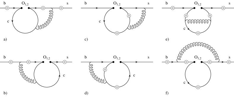
FIG. 1.: Complete list of two-loop Feynman diagrams for $b\rightarrow s\gamma^{*}$ associated with the operators $O_{1}$ and $O_{2}$. The fermions ($b$, $s$ and $c$ quarks) are represented by solid lines, whereas the curly lines represent gluons. The circle-crosses denote the possible locations where the virtual photon (which then splits into a lepton pair) is emitted.

As indicated in this figure, the diagrams associated with $O_{1}$ and $O_{2}$ are topologically identical. They differ only by the color structure. While the matrix elements of the operator $O_{2}$ all involve the color structure

$$\sum_{a}T^{a}T^{a}=C_{F}{\bf 1};\quad C_{F}=\frac{N_{c}^{2}-1}{2N_{c}},$$ (9)

there are two possible color structures for the corresponding diagrams of $O_{1}$, viz.

$$\tau_{1}=\sum_{a,b}T^{a}T^{b}T^{a}T^{b}\quad\text{and}\quad\tau_{2}=\sum_{a,b}T^{a}T^{b}T^{b}T^{a}.$$ (10)

The structure $\tau_{1}$ appears in diagrams 1a)-d) and $\tau_{2}$ in diagrams 1e) and 1f). Using the relation

$\displaystyle\sum_{a}\,T^{a}_{\alpha\beta}T^{a}_{\gamma\delta}=-\frac{1}{2N_{c}}\,\delta_{\alpha\beta}\delta_{\gamma\delta}+\frac{1}{2}\,\delta_{\alpha\delta}\delta_{\beta\gamma},$we find that $\tau_{1}=C_{\tau_{1}}{\bf 1}$ and $\tau_{2}=C_{\tau_{2}}{\bf 1}$ with

$\displaystyle C_{\tau_{1}}=-\frac{N_{c}^{2}-1}{4N_{c}^{2}}\quad\text{and}\quad C_{\tau_{2}}=\frac{\left(N_{c}^{2}-1\right)^{2}}{4N_{c}^{2}}\,.$Inserting $N_{c}=3$, the color factors are $C_{F}=\frac{4}{3},C_{\tau_{1}}=-\frac{2}{9}$ and $C_{\tau_{2}}=\frac{16}{9}$. The contributions from $O_{1}$ are obtained by multiplying those from $O_{2}$ by the appropriate factors, i.e. by $C_{\tau_{1}}/C_{F}=-1/6$ and $C_{\tau_{2}}/C_{F}=4/3$, respectively. In the following descriptions of the individual diagrams we therefore restrict ourselves to those associated with the operator $O_{2}$.

In the current paper we use the $\overline{\text{MS}}$ renormalization scheme which is technically implemented by introducing the renormalization scale in the form $\overline{\mu}^{\,2}=\mu^{2}\exp(\gamma_{E})/(4\pi)$, followed by minimal subtraction. The precise definition of the evanescent operators, which is necessary to fully specify the renormalization scheme, will be given later. The remainder of this section is divided into 8 subsections. Subsections 1-6 deal with the diagrams 1a)-d) which are calculated by means of Mellin-Barnes techniques [45]. Subsection 7 is devoted to the diagrams 1e) which are evaluated by using the heavy mass expansion procedure [46]. Among the diagrams 1f) only the one where the virtual photon is emitted from the charm quark line is non-zero. As it factorizes into two one-loop diagrams, its calculation is straightforward and does not require to be discussed in detail. It is, however, worth mentioning already at this point that it is convenient to omit this diagram in the discussion of the matrix elements of $O_{1}$ and $O_{2}$ and to take it into account together with the virtual corrections to $O_{9}$. Finally, in subsection 8, we give the results for the dimensionally regularized matrix elements $\langle s\ell^{+}\ell^{-}|O_{i}|b\rangle\,(i=1,2)$.

1 The building blocks $I_{\beta}$ and $J_{\alpha\beta}$

For the calculation of diagrams 1a) - d) it is advisable to evaluate the building blocks $I_{\beta}$ and $J_{\alpha\beta}$ first. The corresponding diagrams are depicted in Fig. 2.

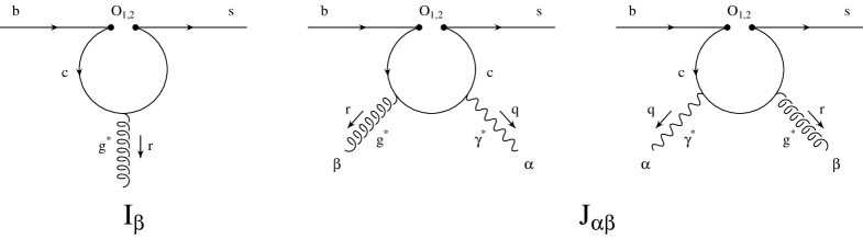
FIG. 2.: The building blocks $I_{\beta}$ and $J_{\alpha\beta}$ which are used for the calculation of the two-loop diagrams 1a)-d). The curly and wavy lines represent gluons and photons, respectively.

After performing a straightforward Feynman parameterization followed by the integration over the loop momentum, the analytic expression for the building block $I_{\beta}$ reads

$$I_{\beta}=-\frac{g_{s}}{4\pi^{2}}\,\Gamma(\epsilon)\,\mu^{2\epsilon}\,e^{\gamma_{E}\epsilon}\,(1-\epsilon)\,e^{i\pi\epsilon}\,\left(r_{\beta}r/-r^{2}\gamma_{\beta}\right)\,L\,\frac{\lambda}{2}\times\\ \int_{0}^{1}\!dx\,\left[x(1-x)\right]^{1-\epsilon}\,\left[r^{2}-\frac{m_{c}^{2}}{x(1-x)}+i\delta\right]^{-\epsilon}\,,$$ (11)

where $r$ is the momentum of the virtual gluon emitted from the $c$-quark loop. The term $i\delta$ is the ”$i\epsilon$-prescription”. In the full two-loop diagrams, the free index $\beta$ will be contracted with the corresponding gluon propagator. Note, that $I_{\beta}$ is gauge invariant in the sense that $r^{\beta}I_{\beta}=0$.

The building block $J_{\alpha\beta}$ is somewhat more complicated. Using the notation introduced by Simma and Wyler [47], it reads

$$J_{\alpha\beta}=\frac{eg_{s}Q_{u}}{16\pi^{2}}\left[E(\alpha,\beta,r)\Delta i_{5}+E(\alpha,\beta,q)\Delta i_{6}-E(\beta,r,q)\frac{r_{\alpha}}{q\!\cdot\!r}\Delta i_{23}\right.\\ \left.-E(\alpha,r,q)\frac{r_{\beta}}{q\!\cdot\!r}\Delta i_{25}-E(\alpha,r,q)\frac{q_{\beta}}{q\!\cdot\!r}\Delta i_{26}-E(\beta,r,q)\frac{q_{\alpha}}{q\!\cdot\!r}\Delta i_{27}\right]\,L\,\frac{\lambda}{2}\,,$$ (12)

where $q$ and $r$ denote the momenta of the (virtual) photon and gluon, respectively. The indices $\alpha$ and $\beta$ will be contracted with the propagators of the photon and the gluon, respectively. The matrix $E(\alpha,\beta,r)$ is defined as

$$E(\alpha,\beta,r)=\frac{1}{2}(\gamma_{\alpha}\gamma_{\beta}r/-r/\gamma_{\beta}\gamma_{\alpha})$$ (13)

and the dimensionally regularized quantities $\Delta i_{k}$ occurring in eq. (12) read

$$\Delta i_{5} = 4\,B^{+}\int_{S}\!dx\,dy\left[4(q\!\cdot\!r)\,x\,y\,(1-x)\epsilon+r^{2}\,x\,(1-x)(1-2\,x)\epsilon\right.$$ (15)

$$\hskip 28.45274pt\left.+q^{2}\,y(2-2\,y+2\,x\,y-x)\epsilon+(1-3x)C\right]\,C^{-1-\epsilon}\,,$$

$$\Delta i_{6} = 4\,B^{+}\int_{S}\!dx\,dy\left[-4(q\!\cdot\!r)\,x\,y\,(1-y)\epsilon-q^{2}\,y\,(1-y)(1-2\,y)\epsilon\right.$$ (17)

$$\hskip 28.45274pt\left.-r^{2}\,x\,(2-2\,x+2\,x\,y-y)\epsilon-(1-3\,y)C\right]\,C^{-1-\epsilon}\,,$$

$$\Delta i_{23} = -\Delta i_{26}=8\,B^{+}(q\!\cdot\!r)\int_{S}\!dx\,dy\,x\,y\,\epsilon\,C^{-1-\epsilon}\,,$$ (18)

$$\Delta i_{25} = -8\,B^{+}(q\!\cdot\!r)\int_{S}\!dx\,dy\,x\,(1-x)\,\epsilon\,C^{-1-\epsilon}\,,$$ (19)

$$\Delta i_{27} = 8\,B^{+}(q\!\cdot\!r)\int_{S}\!dx\,dy\,y\,(1-y)\,\epsilon\,C^{-1-\epsilon}\,,$$ (20)

where $B^{+}=(1+\epsilon)\Gamma(\epsilon)\,e^{\gamma_{E}\epsilon}\mu^{2\epsilon}$ and $C$ is given by

$$C=m_{c}^{2}-2\,x\,y(q\!\cdot\!r)-r^{2}\,x\,(1-x)-q^{2}\,y\,(1-y).$$

The integration over the Feynman parameters $x$ and $y$ is restricted to the simplex $S$, i.e. $y\in[0,1-x]$, $x\in[0,1]$. Due to Ward identities, the quantities $\Delta i_{k}$ are not independent of one another. Namely,

$\displaystyle q^{\alpha}J_{\alpha\beta}=0\quad\text{and}\quad r^{\beta}J_{\alpha\beta}=0$imply that $\Delta i_{5}$ and $\Delta i_{6}$ can be expressed as

$$\Delta i_{5}=\Delta i_{23}+\frac{q^{2}}{q\!\cdot\!r}\Delta i_{27}\,;\quad\Delta i_{6}=\frac{r^{2}}{q\!\cdot\!r}\Delta i_{25}+\Delta i_{26}.$$ (21)

2 General remarks

After inserting the above expressions for the building blocks $I_{\beta}$ and $J_{\alpha\beta}$ into diagrams 1a), b) and 1c), d), respectively, and introducing additional Feynman parameters, we can easily perform the integration over the second loop momentum. The remaining Feynman parameter integrals are, however, non-trivial. In refs. [12] and [48], where the analogous corrections to the processes $b\rightarrow s\gamma$ and $b\rightarrow sg$ were studied, the strategy used to evaluate these integrals is the following:

• The denominators are represented as complex Mellin-Barnes integrals (see below and refs. [12, 48]).

• After interchanging the order of integration and appropriate variable transformations, the Feynman parameter integrals reduce to Euler $\beta$- and $\Gamma$- functions.

• Finally, by Cauchy’s theorem the remaining complex integral over the Mellin variable can be written as a sum over residues taken at certain poles of $\beta$- and $\Gamma$- functions. This leads in a natural way to an expansion in the small ratio $z=m_{c}^{2}/m_{b}^{2}$.

However, this procedure cannot be applied directly in the present case: While the processes $b\rightarrow s\gamma$ and $b\rightarrow sg$ are characterized by the two mass scales $m_{b}$ and $m_{c}$, a third mass scale, viz. $q^{2}$, the invariant mass squared of the lepton pair enters the process $b\rightarrow s\ell^{+}\ell^{-}$. For values of $q^{2}$ satisfying

$\displaystyle\frac{q^{2}}{m_{b}^{2}}<1\quad\text{and}\quad\frac{q^{2}}{4m_{c}^{2}}<1,$most of the diagrams allow a naive Taylor series expansion in $q^{2}$ and the dependence of the charm quark mass can again be calculated by means of Mellin-Barnes representations. This method does not work, however, for the diagram in Fig. 1a) where the photon is emitted from the internal $s$-quark line. Instead, we apply a Mellin-Barnes representation twice, as we discuss in detail in subsection 4. Using these methods, we get the results for diagrams 1a)–d) as an expansion in $\hat{s}=q^{2}/m_{b}^{2}$, $z=m_{c}^{2}/m_{b}^{2}$ and $\hat{s}/(4z)$ as well as $\ln(\hat{s})$ and $\ln(z)$. This implies that our results are meaningful only for small values of $\hat{s}$. Fortunately, this is exactly the range of main theoretical and experimental interest in the phenomenology of the process $b\rightarrow s\ell^{+}\ell^{-}$.

3 Calculation of diagram 1b)

We describe the basic steps of our calculation of the diagram in Fig. 1b) where the photon is emitted from the internal $b$-quark line. Our notations for the momenta are set up in Fig. 3a).

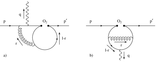
FIG. 3.: a) Momentum flow in diagram 1b), where the virtual photon is emitted from the $b$-quark line (see subsection 3); b) Momentum flow in the vertex correction diagram in Fig. 1e) (see subsection 7).

Inserting the building block $I_{\beta}$ yields the following analytic expression for this diagram:

$$M_{2}[1b]=\frac{i\,e\,Q_{d}\,g_{s}^{2}}{4\pi^{2}}\,C_{F}\,\Gamma(\epsilon)e^{2\gamma_{E}\epsilon}\mu^{4\epsilon}(1-\epsilon)e^{i\pi\epsilon}(4\pi)^{-\epsilon}\int_{0}^{1}\!\,dx\,\frac{[x(1-x)]^{1-\epsilon}}{[r^{2}-m_{c}^{2}/(x(1-x))+i\delta]^{\epsilon}}\\ \int\!\frac{d^{d}r}{(2\pi)^{d}}\,\bar{u}(p^{\prime})\left(r_{\beta}r/-r^{2}\gamma_{\beta}\right)\,L\,\frac{p^{\prime}/+r/+m_{b}}{(p^{\prime}+r)^{2}-m_{b}^{2}}\,\gamma_{\alpha}\,\frac{p/+r/+m_{b}}{(p+r)^{2}-m_{b}^{2}}\,\gamma^{\beta}\,u(p)\cdot\frac{1}{r^{2}}\,.$$ (22)

Applying a Feynman parameterization according to

$$\frac{1}{D_{1}D_{2}D_{3}D_{4}^{\epsilon}}=\frac{\Gamma(3+\epsilon)}{\Gamma(\epsilon)}\,\int_{S}\frac{du\,dv\,dy\,\,y^{\epsilon-1}\,}{\big{[}uD_{1}+vD_{2}+(1-u-v-y)D_{3}+yD_{4}\big{]}^{3+\epsilon}}\,,$$ (23)

with

$$D_{1} =(p^{\prime}+r)^{2}-m_{b}^{2}, D_{2} =(p+r)^{2}-m_{b}^{2},$$ (24)

$$D_{3} =r^{2}, D_{4} =r^{2}-m_{c}^{2}/[x(1-x)],$$ (25)

and performing the integral over the loop momentum $r$, we obtain

$$M_{2}[1b]=-\frac{e\,Q_{d}\,g_{s}^{2}}{64\pi^{4}}(1-\epsilon)C_{F}\,\Gamma(2\epsilon)e^{2\gamma_{E}\epsilon}\mu^{4\epsilon}\times\\ \int\limits^{1}_{0}\!\!dx\,[x(1-x)]^{1-\epsilon}\int_{S}dv\,du\,dy\,y^{\epsilon-1}\,\bar{u}(p^{\prime})\!\left[\frac{P_{1}}{\Delta_{b}^{1+2\epsilon}}+\frac{P_{2}}{\Delta_{b}^{2\epsilon}}+\frac{P_{3}\Delta_{b}}{\Delta_{b}^{2\epsilon}}\right]\,u(p)\,,$$ (26)

where the Feynman parameters $u$, $v$ and $y$ run over the simplex $S$, i.e $u,v,y>0$ and $u+v+y\leq 1$. $P_{1}$, $P_{2}$ and $P_{3}$ are polynomials in the Feynman parameters and the quantity $\Delta_{b}$ reads

$\displaystyle\Delta_{b}=m_{b}^{2}(u+u\,v+v^{2})-q^{2}\,u\,v+\frac{m_{c}^{2}\,y}{x(1-x)}\,.$For $q^{2}\leq m_{b}^{2}$ it is positive in the integration region. Therefore, one is allowed to do a naive Taylor series expansion of the integrand in $q^{2}$. In order to simplify the resulting Feynman parameter integrals, it is convenient to first transform the integration variables $x$, $y$, $u$ and $v$ according to

$$u\rightarrow\frac{(1-v^{\prime})(-1+v^{\prime}+u^{\prime})}{v^{\prime}},\quad v\rightarrow\frac{(1-v^{\prime})(1-u^{\prime})}{v^{\prime}},\quad x\rightarrow x^{\prime},\quad y\rightarrow y^{\prime}v^{\prime}.$$

The integration region of the new variables is given by $u^{\prime}\in[(1-v^{\prime}),1]$ and $v^{\prime},x^{\prime},y^{\prime}\in[0,1]$. Taking the corresponding Jacobian into account and omitting primes in order to simplify the notation, we find

$$M_{2}[1b]=-\frac{e\,Q_{d}\,g_{s}^{2}}{64\pi^{4}}(1-\epsilon)C_{F}\,\Gamma(2\epsilon)e^{2\gamma_{E}\epsilon}\mu^{4\epsilon}\times\\ \int\limits^{1}_{0}\!\!dx\,[x(1-x)]^{1-\epsilon}\int\limits_{0}^{1}\!\!dv\int\limits_{1-v}^{1}\!\!du\int\limits_{0}^{1}\!\!dy\,(v\,y)^{\epsilon-1}\,(1-v)\,\bar{u}(p^{\prime})\!\left[\frac{Q_{1}}{\Delta_{b}^{1+2\epsilon}}+\frac{Q_{2}}{\Delta_{b}^{2\epsilon}}+\frac{Q_{3}\Delta_{b}}{\Delta_{b}^{2\epsilon}}\right]u(p)\,,$$ (27)

where, in terms of the new variables, $\Delta_{b}$ reads

$\displaystyle\Delta_{b}=m_{b}^{2}(1-v)u+q^{2}\frac{(1-v)^{2}(1-v-u)(1-u)}{v^{2}}+m_{c}^{2}\frac{v\,y}{x(1-x)}\,.$$Q_{1}$, $Q_{2}$ and $Q_{3}$ are rational functions in the new Feynman parameters. After performing the Taylor series expansion in $q^{2}$, the remaining integrals are of the form

$$\int\limits_{0}^{1}\!dx\,dv\,dy\int\limits_{1-v}^{1}du\,[x(1-x)]^{1-\epsilon}(v\,y)^{\epsilon-1}(1-v)\frac{1}{v^{m}}\frac{P(x,y,u,v)}{\Delta_{b,0}^{~{}n+2\epsilon}}\,,$$ (28)

where $P(x,y,u,v)$ is a polynomial in $x$, $y$, $u$, $v$; $\Delta_{b,0}=\Delta_{b}(q^{2}=0)$; $n$ and $m$ are non-negative integers. We further follow the strategy used in [12, 48] and represent the denominators $\Delta_{b,0}^{\lambda}$ as Mellin-Barnes integrals. The Mellin-Barnes representation for $(K^{2}-M^{2})^{-\lambda}$ reads ($\lambda>0$)

$$\frac{1}{(K^{2}-M^{2})^{\lambda}}=\frac{1}{(K^{2})^{\lambda}}\,\frac{1}{\Gamma(\lambda)}\,\frac{1}{2\pi i}\,\int_{\gamma}\!ds\,\left(-\frac{M^{2}}{K^{2}}\right)^{s}\Gamma(-s)\,\Gamma(\lambda+s)\,.$$ (29)

The integration path $\gamma$ runs parallel to the imaginary axis and intersects the real axis somewhere between $-\lambda$ and 0. The Mellin-Barnes representation of $\Delta_{b,0}^{\lambda}$ is obtained by making the identifications

$\displaystyle K^{2}\leftrightarrow m_{b}^{2}\,u(1-v)\quad\text{and}\quad M^{2}\leftrightarrow-m_{c}^{2}\,y\,v/[x(1-x)].$Interchanging the order of integration, it is now an easy task to perform the Feynman parameter integrals since the most complicated ones are of the form

$$\int\limits_{0}^{1}\!da\,a^{p(s)}(1-a)^{q(s)}=\beta\big{(}p(s)+1,q(s)+1\big{)}\,.$$ (30)

The integration path $\gamma$ has to be chosen in such a way that the Feynman parameter integrals exist for values of $s\in\gamma$. By inspection of the explicit expressions, one finds that this is the case if the path $\gamma$ is chosen such that $\rm{Re}(s)>-\epsilon$. (Note that in this paper $\epsilon$ is always a positive number). To perform the integration over the Mellin parameter $s$, we close the integration path in the right half-plane and use the residue theorem to identify the integral with the sum over the residues of the poles located at

$$s = 0,~{}1,~{}2,~{}3,~{}........$$ (31)

$$s = 1-\epsilon,~{}2-\epsilon,~{}3-\epsilon,~{}.......$$ (32)

$$s = 1-2\epsilon,~{}2-2\epsilon,~{}3-2\epsilon,~{}.......,$$ (33)

$$s = 1/2-2\epsilon,~{}3/2-2\epsilon,~{}5/2-2\epsilon,~{}.......\quad$$ (34)

In view of the factor $(m_{c}^{2}/m_{b}^{2})^{s}$ stemming from the Mellin-Barnes formula (29), the evaluation of the residues at the pole positions listed in eq. (31) corresponds directly to an expansion in $z=m_{c}^{2}/m_{b}^{2}$. Note, that closing the integration contour in the right half-plane yields an overall minus sign due to the clockwise orientation of the integration path. After expanding in $\epsilon$, we get the form factors of $M_{2}[1b]$ (see eq. (6)) as an expansion of the form

$$F_{2}^{(7,9)}[1b]=\sum_{i,l,m}c^{(7,9)}_{2,ilm}\,\hat{s}^{i}\,z^{l}\,\ln^{m}(z)\,,$$ (35)

where $i$ and $m$ are non-negative integers and $l$ is a natural multiple of $\frac{1}{2}$ (see eq. (31)). Furthermore, the power $m$ of $\ln(z)$ is bounded by four, independent of the values of $i$ and $l$. This becomes clear if we consider the structure of the poles. There are three poles in $s$ located near any natural number $k$, viz. at $s=k$, $s=k-\epsilon$ and $s=k-2\epsilon$. Taking the residue at one of them yields a term proportional to $1/\epsilon^{2}$ from the other two poles. In addition, there can be an explicit $1/\epsilon^{2}$ term from the integration over the two loop momenta. Therefore, the most singular term can be of order $1/\epsilon^{4}$ and, after expanding in $\epsilon$, the highest possible power of $\ln(z)$ is four.

4 Calculation of diagram 1a)

To calculate the diagram in Fig. 1a) where the photon is emitted from the internal $s$-quark, we proceed in a similar way as in the previous subsection, i.e., we insert the building block $I_{\beta}$, introduce three additional Feynman parameters and integrate over the loop momentum $r$. The characteristic denominator $\Delta_{a}$ is of the form

$\displaystyle\Delta_{a}=\left(A\,m_{b}^{2}+B\,q^{2}+C\,m_{c}^{2}+i\delta\right)$and occurs with powers $2\epsilon$ or $1+2\epsilon$. The coefficients $A$, $B$ and $C$ are functions of the Feynman parameters. After suitable transformations, they read

$\displaystyle A=u\,v(1-v);\quad B=u\,v^{2}(1-u);\quad C=-\frac{y(1-v)}{x(1-x)}\,,$with $u,~{}x,~{}y,~{}v\in[0,1]$. From this we conclude that the result of this diagram is not analytic in $q^{2}$. We are therefore not allowed to Taylor expand the integrand. Instead, we apply the Mellin-Barnes representation twice and write

$$\frac{1}{\Delta_{a}^{\lambda}}=\frac{1}{\left(B\,q^{2}\right)^{\lambda}}\int_{\gamma}ds\int_{\gamma^{\prime}}ds^{\prime}\,\frac{\Gamma(s+\lambda)\,\Gamma(-s^{\prime})\,\Gamma(s^{\prime}-s)\,e^{i\pi s^{\prime}}}{(2\pi i)^{2}\,\Gamma(\lambda)}\left[\frac{A\,m_{b}^{2}}{B\,q^{2}}\right]^{s}\left[-\frac{C\,m_{c}^{2}}{A\,m_{b}^{2}}\right]^{s^{\prime}}\,.$$ (36)

The integration paths $\gamma$ and $\gamma^{\prime}$ are again parallel to the imaginary axis and $-\lambda<\mbox{Re}(s)<\mbox{Re}(s^{\prime})<0$. $\lambda$ takes one of the two values $2\epsilon$ and $1+2\epsilon$. We have written eq. (36) in such a way that non-integer powers appear only for positive numbers, i.e. we made use of the formula

$\displaystyle(x\pm i\delta)^{\alpha}=e^{\pm i\pi\alpha}(-x\mp i\delta)^{\alpha}\,.$As in the previous subsection, the exact positions of the integration paths $\gamma$ and $\gamma^{\prime}$ are dictated by the condition that the Feynman parameter integrals exist for values of $s$ and $s^{\prime}$ lying thereon. For $\lambda=2\epsilon$, we find that these integrals exist if

$\displaystyle-\epsilon<\mbox{Re}(s)<\mbox{Re}(s^{\prime})<0.$Closing the integration contour for the $s$- and $s^{\prime}$-integration in the left and right half-plane, respectively, and applying the residue theorem results in an expansion in $\hat{s}$ and $z$. As $\rm{Re}(s^{\prime})>\rm{Re}(s)$, the term $\Gamma(s^{\prime}-s)$ in eq. (36) does not generate any poles. For $\lambda=2\epsilon$, the poles which have to be taken into account are located at

$$s^{\prime} =1-\epsilon,~{}2-\epsilon,~{}3-\epsilon,~{}...... s =-\epsilon,~{}-1-\epsilon,~{}-2-\epsilon,~{}......$$ (37)

$$s^{\prime} =1-2\epsilon,~{}2-2\epsilon,~{}3-2\epsilon,~{}...... s =-2\epsilon,~{}-1-2\epsilon,~{}-2-2\epsilon,~{}......$$ (38)

$$s^{\prime} =0,~{}1,~{}2,~{}......$$ (39)

For $\lambda=1+2\epsilon$, we find that the Feynman parameter integrals exist if

$\displaystyle-\epsilon<\mbox{Re}(s^{\prime})<0\quad\rm{and}\quad-1-\epsilon<\mbox{Re}(s)<-2\epsilon\,.$This condition implies that the poles at $s=-\epsilon,-2\epsilon$ in the above list must not be taken into account when applying the residue theorem.

The final result for the form factors (eq.(6)) of this diagram is of the form

$$F_{2}^{(7,9)}[1a]=\sum_{i,j,l,m}c^{(7,9)}_{i,j,l,m}\,\hat{s}^{i}\,\ln^{j}(\hat{s})\,z^{l}\,\ln^{m}(z)\,,$$ (40)

where $i,~{}j,~{}l$ and $m$ all are non-negative integers. The remaining four diagrams in Fig. 1a) and b) exhibit no further difficulties.

5 Calculation of diagrams 1c)

Inserting the building block $J_{\alpha\beta}$ allows us to calculate directly the sum of the two diagrams shown in Fig. 1c). After performing the second loop integral, one obtains

$$M_{2}[1c]=\frac{eQ_{u}g_{s}^{2}C_{F}}{256\pi^{4}}(1+\epsilon)\,\Gamma(2\epsilon)e^{2\gamma_{E}\epsilon}\mu^{4\epsilon}e^{2i\pi\epsilon}\\ \int dx\,dy\,du\,dv\,\frac{v^{\epsilon}(1-u)^{1+\epsilon}(1-x)}{[x(1-x)]^{1+\epsilon}}\,\bar{u}(p^{\prime})\left[\frac{P_{1}}{\Delta_{c}^{1+2\epsilon}}+\frac{P_{2}}{\Delta_{c}^{2\epsilon}}+\frac{P_{3}\Delta_{c}}{\Delta_{c}^{2\epsilon}}\right]u(p)\,,$$ (41)

where $P_{1}$, $P_{2}$ and $P_{3}$ are polynomials in the Feynman parameters, which all run in the interval [0,1]. $\Delta_{c}$ reads (using $v^{\prime}=v(1-u)$)

$\displaystyle\Delta_{c}=m_{b}^{2}\,u\,v^{\prime}\,y-q^{2}\,y\,v^{\prime}\left(u+y\,v^{\prime}\right)-\frac{v^{\prime}}{x(1-x)}\left[m_{c}^{2}-q^{2}\,y(1-x)\left(1-y(1-x)\right)\right]\,.$Note that we do not expand in $q^{2}$ at this stage of the calculation. Instead, we use the Mellin-Barnes representation (29) with the identification

$\displaystyle K^{2}\leftrightarrow m_{b}^{2}\,u\,v^{\prime}\,y\quad\text{and}\quad M^{2}\leftrightarrow q^{2}\,y\,v^{\prime}\left(u+y\,v^{\prime}\right)+\frac{v^{\prime}}{x(1-x)}\left[m_{c}^{2}-q^{2}\,y(1-x)\left(1-y(1-x)\right)\right]\,.$This representation does a good job, since $\left(-M^{2}/K^{2}\right)^{s}$ turns out to be analytic in $q^{2}$ for $\hat{s}<4z$, as in this range $M^{2}/K^{2}$ is positive for all values of the Feynman parameters. We therefore do the Taylor expansion with respect to $q^{2}$ only at this level. Evaluating the Feynman parameter integrals as well as the Mellin-Barnes integral, we find the result as an expansion in $z$ and $\hat{s}/(4z)$ which can be cast into the general form

$$F_{2}^{(7,9)}[1c]=\sum_{i,l,m}c_{2,ilm}^{(7,9)}\,\hat{s}^{i}\,z^{l}\,\ln^{m}(z),$$ (42)

where $i$ and $m$ are non-negative integers and $l=-i,~{}-i+\frac{1}{2},~{}-i+1,~{}....$.

6 Calculation of diagrams 1d)

After inserting the building block $J_{\alpha\beta}$ and performing the second loop integral, the sum of the diagrams in Fig. 1d) yields

$$M_{2}[1d]=\frac{eQ_{u}g_{s}^{2}C_{F}}{256\pi^{4}}(1+\epsilon)\,\Gamma(2\epsilon)e^{2\gamma_{E}\epsilon}\mu^{4\epsilon}\\ \int\limits_{S}dx\,dy\,\int\limits_{S}du\,dv\,\frac{v^{\epsilon}}{[x(1-x)]^{1+\epsilon}}\,\bar{u}(p^{\prime})\left[\frac{P_{1}}{\Delta_{d}^{1+2\epsilon}}+\frac{P_{2}}{\Delta_{d}^{2\epsilon}}+\frac{P_{3}\Delta_{d}}{\Delta_{d}^{2\epsilon}}\right]u(p)\,,$$ (43)

where $P_{1}$, $P_{2}$ and $P_{3}$ are polynomials in the Feynman parameters $x$, $y$, $u$ and $v$. The parameters $(x,y)$ and $(u,v)$ run in their respective simplex. The quantity $\Delta_{d}$ reads

$\displaystyle\Delta_{d}=m_{b}^{2}\,u\left(u+\frac{y\,v}{1-x}\right)+q^{2}\,y\,v\left[\frac{y\,v}{(1-x)^{2}}+\frac{u}{1-x}-\frac{(1-y)}{x(1-x)}\right]+\frac{m_{c}^{2}\,v}{x(1-x)}\,.$Next, we use the Mellin-Barnes representation (29) with the identification

$\displaystyle K^{2}\leftrightarrow m_{b}^{2}\,u\left(u+\frac{y\,v}{1-x}\right)\,;\quad M^{2}\leftrightarrow q^{2}\,y\,v\left[\frac{y\,v}{(1-x)^{2}}+\frac{u}{1-x}-\frac{(1-y)}{x(1-x)}\right]+\frac{m_{c}^{2}\,v}{x(1-x)}\,.$Again, $\left(-M^{2}/K^{2}\right)^{s}$ is analytic in $q^{2}$ for $\hat{s}<4z$, what allows us to perform a Taylor series expansion with respect to $q^{2}$. In order to perform the integrations over the Feynman parameters, we make suitable substitutions, e.g.

$$x\rightarrow x^{\prime},\quad y\rightarrow\frac{(1-x^{\prime})(y^{\prime}-(1-v^{\prime}))}{v^{\prime}},\quad v\rightarrow u^{\prime}v^{\prime},\quad u\rightarrow u^{\prime}(1-v^{\prime}).$$ (44)

The new variables $x^{\prime},u^{\prime},v^{\prime}$ run in the interval $[0,1]$, while $y^{\prime}$ varies in $[1-v^{\prime},1]$. Evaluating the integrals over the Feynman and Mellin parameters, we find the result as an expansion in $z$ and $\hat{s}/(4z)$ which can be cast into the general form

$$F_{2}^{(7,9)}[1d]=\sum_{i,l,m}c_{2,ilm}^{(7,9)}\,\hat{s}^{i}\,z^{l}\,\ln^{m}(z)\,.$$ (45)

$i$ and $m$ are non-negative integers and $l=-i,~{}-i+\frac{1}{2},~{}-i+1,~{}....$.

7 Calculation of diagram 1e)

We consider one of the diagrams in Fig. 1e) in some detail and redraw it in Fig. 3b). The matrix element is proportional to $1/\Delta_{e}$, where

$$\Delta_{e}=[(l-r)^{2}-m_{c}^{2}]\,[(l-q-r)^{2}-m_{c}^{2}]\,[(l-q)^{2}-m_{c}^{2}]\,[l^{2}-m_{c}^{2}]\,r^{2}\,.$$ (46)

$q$ is the four-momentum of the off-shell photon, while $l$ and $r$ denote loop momenta. As $q^{2}<4m_{c}^{2}$ in our application, we use the heavy mass expansion (HME) technique [46] to evaluate this diagram. In the present case, as the gluon is massless, the HME boils down to a naive Taylor series expansion of the diagram (before loop integrations) in the four-momentum $q$. Expanding $1/\Delta_{e}$ in $q$, we obtain

$$\frac{1}{\Delta_{e}}=\sum\limits_{n,m,i,j,k}C_{e}(n,m,i,j,k)\frac{(q^{2})^{i}(q\cdot r)^{j}(q\cdot l)^{k}}{r^{2}\,[l^{2}-m_{c}^{2}]^{n}\,[(l-r)^{2}-m_{c}^{2}]^{m}}\quad.$$ (47)

Using the Feynman parameterization

$$\frac{1}{[l^{2}-m_{c}^{2}]^{n}\,[(l-r)^{2}-m_{c}^{2}]^{m}}=\frac{\Gamma(n+m)}{\Gamma(n)\Gamma(m)}\int\limits_{0}^{1}\frac{v^{m-1}(1-v)^{n-1}}{[l^{2}-2v(l\cdot r)-m_{c}^{2}+vr^{2}]^{n+m}}\,dv\,,$$ (48)

we can perform the integration over the loop momentum $l$. The integral over the loop momentum $r$ can be done using the parameterization

$$\frac{1}{r^{2}}\left(\frac{1}{r^{2}-\frac{m_{c}^{2}}{v(1-v)}}\right)^{p}=\frac{\Gamma(1+p)}{\Gamma(p)}\int\limits_{0}^{1}\frac{u^{p-1}}{\left(r^{2}-\frac{u\,m_{c}^{2}}{v(1-v)}\right)^{p+1}}\,du\,.$$ (49)

The remaining integrals over the Feynman parameters $u$ and $v$ all have the form of eq. (30) and can be performed easily. The other two diagrams in Fig. 1e) where the virtual photon is emitted from the charm quark can be evaluated in a similar way. The diagrams where the photon is radiated from the $b$-quark or the $s$-quark vanish.

As the results for the sum of all the diagrams in Fig. 1e) are compact, we explicitly give their contribution to the form factors $F_{a}^{(j)}$ ($a=1,2$; $j=7,9$). We obtain $F_{a}^{(7)}[1e]=0$, $F_{1}^{(9)}[1e]=\frac{4}{3}\,F_{2}^{(9)}[1e]$ and

$$F_{2}^{(9)}[1e] = \left(\frac{\mu}{m_{c}}\right)^{4\epsilon}\,\frac{1}{\epsilon}\,\left[\frac{8}{3}+\frac{128}{45}\,\left(\frac{\hat{s}}{4z}\right)+\frac{256}{105}\left(\frac{\hat{s}}{4z}\right)^{2}+\frac{2048}{945}\left(\frac{\hat{s}}{4z}\right)^{3}\right]$$ (51)

$$-\left[\frac{124}{27}+\frac{12416}{3645}\,\left(\frac{\hat{s}}{4z}\right)+\frac{11072}{42525}\left(\frac{\hat{s}}{4z}\right)^{2}-\frac{4971776}{4465125}\left(\frac{\hat{s}}{4z}\right)^{3}\right]\,.$$

8 Unrenormalized form factors of $O_{1}$ and $O_{2}$

We stress that the diagram 1f) where the virtual photon is emitted from the charm quark line is the only one in Fig. 1 which suffers from infrared and collinear singularities. As this diagram can easily be combined with diagram 4b) associated with the operator $O_{9}$, we take it into account only in section IV A where the virtual corrections to $O_{9}$ are discussed.

The unrenormalized form factors $F^{(7,9)}_{a}$ of $\langle s\ell^{+}\ell^{-}|O_{a}|b\rangle$ $(a=1,2)$, corresponding to diagrams 1a)–1e), are obtained in the form

$\displaystyle F^{(7,9)}_{a}=\sum_{i,j,l,m}c_{a,ijlm}^{(7,9)}\,\hat{s}^{i}\,\ln^{j}(\hat{s})\,z^{l}\,\ln^{m}(z),$where $i,~{}j$ and $m$ are non-negative integers and $l=-i,~{}-i+\frac{1}{2},~{}-i+1,~{}....$. We keep the terms with $i$ and $l$ up to 3, after checking that higher order terms are small for $0.05\leq\hat{s}\leq 0.25$, the range considered in this paper. As we will give the full results for the counterterm contributions to the form factors in section III B and the renormalized form factors in section III C and in appendix B, it is not necessary to explicitly present the somewhat lengthy expressions for the unrenormalized form factors. But, in order to demonstrate the cancellation of ultraviolet singularities in the next section, we list the divergent parts of the unrenormalized form factors: $F_{1}^{(7)}$, $F_{1}^{(9)}$, $F_{2}^{(7)}$ and $F_{2}^{(9)}$:

$$F^{(9)}_{2,\text{div}} = \frac{128}{81\,\epsilon^{2}}-\frac{4}{25515\,\epsilon}\,\left(1890+1260\,i\pi+5040\,L_{\mu}-1260\,L_{s}+252\,\hat{s}+27\,\hat{s}^{2}+4\,\hat{s}^{3}\right)$$ (53)

$$+\frac{8}{2835\,\epsilon}\,\left(420+2520\,L_{\mu}-1260\,L_{z}+2016\left(\frac{\hat{s}}{4z}\right)+1296\left(\frac{\hat{s}}{4z}\right)^{2}+1024\left(\frac{\hat{s}}{4z}\right)^{3}\right)\,,$$

$$F^{(7)}_{2,\text{div}} = \frac{92}{81\,\epsilon}\,,$$ (54)

$$F_{1,\text{div}}^{(9)} -\frac{64}{243\,\epsilon^{2}}+\frac{2}{76545\,\epsilon}\left(1890+1260\,i\pi+5040\,L_{\mu}-1260\,L_{s}+252\,\hat{s}+27\,\hat{s}^{2}+4\,\hat{s}^{3}\right)$$ ⁼ (56)

$$-\frac{4}{8505\,\epsilon}\left(-8085+2520\,L_{\mu}-1260\,L_{z}-7056\left(\frac{\hat{s}}{4z}\right)-6480\left(\frac{\hat{s}}{4z}\right)^{2}-5888\left(\frac{\hat{s}}{4z}\right)^{3}\right)\,,$$

$$F_{1,\text{div}}^{(7)} = -\frac{46}{243\,\epsilon}\,,$$ (57)

where $L_{s}=\ln(\hat{s})$, $L_{z}=\ln(z)$, $L_{\mu}=\ln\left(\frac{\mu}{m_{b}}\right)$ and $z=m_{c}^{2}/m_{b}^{2}$.

B ${\mathcal{O}}(\alpha_{s})$ counterterms to $O_{1}$ and $O_{2}$

So far, we have calculated the two-loop matrix elements $\langle s\ell^{+}\ell^{-}|C_{i}\,O_{i}|b\rangle$ ($i=1,2$). As the operators mix under renormalization, there are additional contributions proportional to $C_{i}$. These counterterms arise from the matrix elements of the operators

$$\sum_{j=1}^{12}\delta Z_{ij}O_{j}\,,\quad i=1,2,$$ (58)

where the operators $O_{1}$–$O_{10}$ are given in eq. (2). $O_{11}$ and $O_{12}$ are evanescent operators, i.e., operators which vanish in $d=4$ dimensions. In principle, there is some freedom in the choice of the evanescent operators. However, as we want to combine our matrix elements with the Wilson coefficients calculated by Bobeth et al. [41], we must use the same definitions:

$$O_{11} =\left(\bar{s}_{L}\gamma_{\mu}\gamma_{\nu}\gamma_{\sigma}T^{a}c_{L}\right)\left(\bar{c}_{L}\gamma^{\mu}\gamma^{\nu}\gamma^{\sigma}T^{a}b_{L}\right)-16\,O_{1}\,,$$ (59)

$$O_{12} =\left(\bar{s}_{L}\gamma_{\mu}\gamma_{\nu}\gamma_{\sigma}c_{L}\right)\left(\bar{c}_{L}\gamma^{\mu}\gamma^{\nu}\gamma^{\sigma}b_{L}\right)-16\,O_{2}\,.$$ (60)

The operator renormalization constants $Z_{ij}=\delta_{ij}+\delta Z_{ij}$ are of the form

$$\delta Z_{ij}=\frac{\alpha_{s}}{4\pi}\left(a_{ij}^{01}+\frac{1}{\epsilon}a_{ij}^{11}\right)+\frac{\alpha_{s}^{2}}{(4\pi)^{2}}\left(a_{ij}^{02}+\frac{1}{\epsilon}a_{ij}^{12}+\frac{1}{\epsilon^{2}}a_{ij}^{22}\right)+{\mathcal{O}}(\alpha_{s}^{3}).$$ (61)

Most of the coefficients $a_{ij}^{lm}$ needed for our calculation are given in ref. [41]. As some are new (or not explicitly given in [41]), we list those for $i=1,~{}2$ and $j=1,...,~{}12$:

$$\hat{a}^{11}=\left(\begin{array}[]{cccccccccccc}-2&\frac{4}{3}&0&-\frac{1}{9}&0&0&0&0&-\frac{16}{27}&0&\frac{5}{12}&\frac{2}{9}\\ \\ 6&0&0&\frac{2}{3}&0&0&0&0&-\frac{4}{9}&0&1&0\end{array}\right),\begin{array}[]{lll}a^{12}_{17}=-\frac{58}{243}\,,&a^{12}_{19}=-\frac{64}{729}\,,&a^{22}_{19}=\frac{1168}{243}\,,\\ \\ a^{12}_{27}=\frac{116}{81}\,,&a^{12}_{29}=\frac{776}{243}\,,&a^{22}_{29}=\frac{148}{81}\,.\end{array}$$ (62)

We denote the counterterm contributions to $b\rightarrow s\ell^{+}\ell^{-}$ which are due to the mixing of $O_{1}$ or $O_{2}$ into four-quark operators by $F_{i\rightarrow\rm{4quark}}^{\rm{ct}(7)}$ and $F_{i\rightarrow\rm{4quark}}^{\rm{ct}(9)}$. They can be extracted from the equation

$$\sum_{j}\left(\frac{\alpha_{s}}{4\pi}\right)\,\frac{1}{\epsilon}\,a_{ij}^{11}\langle s\ell^{+}\ell^{-}|O_{j}|b\rangle_{\text{1-loop}}=-\left(\frac{\alpha_{s}}{4\pi}\right)\,\left[F_{i\rightarrow\rm{4quark}}^{\rm{ct}(7)}\langle\widetilde{O}_{7}\rangle_{\text{tree}}+F_{i\rightarrow\rm{4quark}}^{\rm{ct}(9)}\langle\widetilde{O}_{9}\rangle_{\text{tree}}\right]\,,$$ (63)

where $j$ runs over the four-quark operators. As certain entries of $\hat{a}^{11}$ are zero, only the one-loop matrix elements of $O_{1}$, $O_{2}$, $O_{4}$, $O_{11}$ and $O_{12}$ are needed. In order to keep the presentation transparent, we relegate their explicit form to appendix A.

The counterterms which are related to the mixing of $O_{i}$ ($i=1,2$) into $O_{9}$ can be split into two classes: The first class consists of the one-loop mixing $O_{i}\rightarrow O_{9}$, followed by taking the one-loop corrected matrix element of $O_{9}$. It is obvious that this class contributes to the renormalization of diagram 1f). As we decided to treat diagram 1f) only in section IV A (when discussing virtual corrections to $O_{9}$), we proceed in the same way with the counterterm just mentioned. There is, however, a second class of counterterm contributions due to $O_{i}\rightarrow O_{9}$ mixing. These contributions are generated by two-loop mixing of $O_{2}$ into $O_{9}$ as well as by one-loop mixing and one-loop renormalization of the $g_{s}$ factor in the definition of the operator $O_{9}$. We denote the corresponding contribution to the counterterm form factors by $F_{i\rightarrow 9}^{\rm{ct}(7)}$ and $F_{i\rightarrow 9}^{\rm{ct}(9)}$. We obtain

$$F_{i\rightarrow 9}^{\rm{ct}(9)}=-\left(\frac{a_{i9}^{22}}{\epsilon^{2}}+\frac{a_{i9}^{12}}{\epsilon}\right)-\frac{a_{i9}^{11}\,\beta_{0}}{\epsilon^{2}}\,;\quad F_{i\rightarrow 9}^{\rm{ct}(7)}=0\,,$$ (64)

where we made use of the renormalization constant $Z_{g_{s}}$ given by

$$Z_{g_{s}}=1-\frac{\alpha_{s}}{4\pi}\,\frac{\beta_{0}}{2}\,\frac{1}{\epsilon}\,;\quad\beta_{0}=11-\frac{2}{3}N_{f}\,;\quad N_{f}=5\,.$$ (65)

Besides the contribution from operator mixing, there are ordinary QCD counterterms. The renormalization of the charm quark mass is taken into account by replacing $m_{c}$ through $Z_{m_{c}}\cdot m_{c}$ in the one-loop matrix elements of $O_{1}$ and $O_{2}$ (see appendix A). We denote the corresponding contribution to the counterterm form factors by $F_{i,m_{c}\text{ren}}^{\rm{ct}(7)}$ and $F_{i,m_{c}\text{ren}}^{\rm{ct}(9)}$. We obtain

$$F_{1,m_{c}\text{ren}}^{\rm{ct}(7)}=F_{2,m_{c}\text{ren}}^{\rm{ct}(7)}=0\,;\quad F_{1,m_{c}\text{ren}}^{\rm{ct}(9)}=\frac{4}{3}F_{2,m_{c}\text{ren}}^{\rm{ct}(9)}$$ (66)

$$F_{2,m_{c}\text{ren}}^{\rm{ct}(9)} = \left[-\frac{32}{945\epsilon}\left(105+84\left(\frac{\hat{s}}{4z}\right)+72\left(\frac{\hat{s}}{4z}\right)^{2}+64\left(\frac{\hat{s}}{4z}\right)^{3}\right)\right.$$ (67)

$$- \left.\frac{32}{2835}\left(105+1260\ln{\frac{\mu}{m_{c}}}+\left(\frac{\hat{s}}{4z}\right)\left(336+1008\ln{\frac{\mu}{m_{c}}}\right)+\left(\frac{\hat{s}}{4z}\right)^{2}\left(396+864\ln{\frac{\mu}{m_{c}}}\right)\right.\right.$$ (68)

$$+ \left.\left.\left(\frac{\hat{s}}{4z}\right)^{3}\left(416+768\ln{\frac{\mu}{m_{c}}}\right)\right)\right]\,,$$ (69)

where we have used the pole mass definition of $m_{c}$ which is characterized by the renormalization constant

$$Z_{m}=1-\frac{\alpha_{s}}{4\pi}\frac{4}{3}\left(\frac{3}{\epsilon}+6\ln\left(\frac{\mu}{m}\right)+4\right).$$ (70)

If one wishes to express the results for $F_{i,m_{c}\text{ren}}^{\rm{ct}(9)}$ in terms of the $\overline{\rm{MS}}$ definition of the charm quark mass, the expressions in eqs. (66) get changed according to

$$F_{i,m_{c}\text{ren}}^{\rm{ct}(9)}\rightarrow F_{i,m_{c}\text{ren}}^{\rm{ct}(9)}+\Delta F_{i,m_{c}\text{ren}}^{\rm{ct}(9)}\,,$$ (71)

where $\Delta F_{i,m_{c}\text{ren}}^{\rm{ct}(9)}$ reads

$$\Delta F_{1,m_{c}\text{ren}}^{\rm{ct}(9)}=\frac{4}{3}\Delta F_{2,m_{c}\text{ren}}^{\rm{ct}(9)}$$ (72)

$$\Delta F_{2,m_{c}\text{ren}}^{\rm{ct}(9)} = \frac{64}{945}\,\left(105+84\left(\frac{\hat{s}}{4z}\right)+72\left(\frac{\hat{s}}{4z}\right)^{2}+64\left(\frac{\hat{s}}{4z}\right)^{3}\right)\,\left(\ln\frac{\mu}{m_{c}}+\frac{2}{3}\right)\,.$$ (73)

We stress at this point that we always use the pole mass definition in the following, i.e., eqs. (66) for $F_{i,m_{c}\text{ren}}^{\rm{ct}(j)}$.

The total counterterms $F_{i}^{\rm{ct}(j)}$ ($i=1,2$; $j=7,9$) which renormalize diagrams 1a)–1e) are given by

$$F_{i}^{\rm{ct}(j)}=F_{i\rightarrow\rm{4quark}}^{\rm{ct}(j)}+F_{i\rightarrow 9}^{\rm{ct}(j)}+F_{i,m_{c}\text{ren}}^{\rm{ct}(j)}\,.$$ (74)

Explicitly, they read

$$F_{2}^{\rm{ct}(9)} = -F_{2,\,\text{div}}^{(9)}-\frac{4}{25515}\left[5740+2520\,\pi^{2}-840\,i\pi\right.$$ (75)

$$+ \left.840\,L_{\mu}\left(19-3\,i\pi-54\,L_{z}+48\,L_{\mu}\right)+3780\,L_{z}(-2+3\,L_{z})\right.$$ (76)

$$+ \left.420\,L_{s}(3\,i\pi+2+6\,L_{\mu})-630\,L_{s}^{2}+252\,\hat{s}(1-2\,L_{\mu})-54\,L_{\mu}\,\hat{s}^{2}-2\,\hat{s}^{3}(1+4\,L_{\mu})\right.$$ (77)

$$+ \left.6048\left(\frac{\hat{s}}{4z}\right)\left(18\,L_{\mu}-9\,L_{z}-1\right)+7776\left(\frac{\hat{s}}{4z}\right)^{2}(10\,L_{\mu}-5\,L_{z}+3)\right.$$ (78)

$$+ \left.1536\left(\frac{\hat{s}}{4z}\right)^{3}(42\,L_{\mu}-21\,L_{z}+19)\right]\,,$$ (79)

$$F_{2}^{\rm{ct}(7)} = -F_{2,\,\text{div}}^{(7)}+\frac{2}{2835}\left(840\,L_{\mu}+70\,\hat{s}+7\,\hat{s}^{2}+\hat{s}^{3}\right)\,,$$ (80)

$$F_{1}^{\rm{ct}(9)} = -F_{1,\,\text{div}}^{(9)}+\frac{2}{76545}\left[-62300-840\,i\pi+2520\,\pi^{2}\right.$$ (81)

$$+ \left.840\,L_{\mu}(-3\,i\pi-54\,L_{z}+48\,L_{\mu}-791)+3780\,L_{z}(3\,L_{z}+88)\right.$$ (82)

$$+ \left.420\,L_{s}(3\,i\pi+2+6\,L_{\mu})-630\,L_{s}^{2}+\hat{s}(252-504\,L_{\mu})-54\,\hat{s}^{2}\,L_{\mu}-2\,\hat{s}^{3}(1+4\,L_{\mu})\right.$$ (83)

$$- \left.6048\left(\frac{\hat{s}}{4z}\right)(28+90\,L_{\mu}-45\,L_{z})-7776\left(\frac{\hat{s}}{4z}\right)^{2}(27+62\,L_{\mu}-31\,L_{z})\right.$$ (84)

$$- \left.768\left(\frac{\hat{s}}{4z}\right)^{3}(295+564\,L_{\mu}-282\,L_{z})\right]\,,$$ (85)

$$F_{1}^{\rm{ct}(7)} = -F_{1,\,\text{div}}^{(7)}-\frac{1}{8505}\left(840\,L_{\mu}+70\,\hat{s}+7\,\hat{s}^{2}+\hat{s}^{3}\right)\,.$$ (86)

The divergent parts of these counterterms are, up to a sign, identical to those of the unrenormalized matrix elements given in eq. (53), which proves the cancellation of ultraviolet singularities.

As mentioned before, we will take diagram 1f) into account only in section IV A. The same holds for the counterterms associated with the $b$- and $s$-quark wave function renormalization and, as mentioned earlier in this subsection, the ${\mathcal{O}}(\alpha_{s})$ correction to the matrix element of $\delta Z_{i9}O_{9}$. The sum of these contributions is

$\displaystyle\delta\bar{Z}_{\psi}\langle O_{i}\rangle_{\text{1-loop}}+\frac{\alpha_{s}}{4\pi}\,\frac{a_{i9}^{11}}{\epsilon}\,\left[\delta\bar{Z}_{\psi}\langle O_{9}\rangle_{\text{tree}}+\langle O_{9}\rangle_{\text{1-loop}}\right]\,,\quad\delta\bar{Z}_{\psi}=\sqrt{Z_{\psi}(m_{b})Z_{\psi}(m_{s})}-1,$and provides the counterterm that renormalizes diagram 1f). We use on-shell renormalization for the external $b$- and $s$-quark. In this scheme the field strength renormalization constants are given by

$$Z_{\psi}(m)=1-\frac{\alpha_{s}}{4\pi}\,\frac{4}{3}\,\left(\frac{\mu}{m}\right)^{2\epsilon}\left(\frac{1}{\epsilon}+\frac{2}{\epsilon_{\text{IR}}}+4\right).$$ (87)

So far, we have discussed the counterterms which renormalize the ${\mathcal{O}}(\alpha_{s})$ corrected matrix elements $\langle s\ell^{+}\ell^{-}|O_{i}|b\rangle$ ($i=1,2$). The corresponding one-loop matrix elements (of order ${\mathcal{O}}(\alpha_{s}^{0})$) are renormalized by adding the counterterms

$\displaystyle\frac{\alpha_{s}}{4\pi}\,\frac{a_{i9}^{11}}{\epsilon}\,\langle O_{9}\rangle_{\text{tree}}\,.$

C Renormalized form factors of $O_{1}$ and $O_{2}$

We decompose the renormalized matrix elements of $O_{i}$ ($i=1,2$) as

$$\langle s\ell^{+}\ell^{-}|C_{i}^{(0)}O_{i}|b\rangle=C_{i}^{(0)}\left(-\frac{\alpha_{s}}{4\pi}\right)\left[F_{i}^{(9)}\langle\widetilde{O}_{9}\rangle_{\text{tree}}+F_{i}^{(7)}\langle\widetilde{O}_{7}\rangle_{\text{tree}}\right],$$ (88)

where $\widetilde{O}_{9}=\frac{\alpha_{s}}{4\pi}\,O_{9}$ and $\widetilde{O}_{7}=\frac{\alpha_{s}}{4\pi}\,O_{7}$. The form factors $F_{i}^{(9)}$ and $F_{i}^{(7)}$, expanded up to $\hat{s}^{3}$ and $z^{3}$, of the renormalized sum of diagrams 1a)-e) read ($L_{c}=\ln m_{c}/m_{b}=\ln\hat{m}_{c}=L_{z}/2$)

$$F_{1}^{(9)}=\left(-\frac{1424}{729}+\frac{16}{243}\,i\pi+\frac{64}{27}\,L_{c}\right)L_{\mu}-\frac{16}{243}\,L_{\mu}\,L_{s}+\left(\frac{16}{1215}-\frac{32}{135}\,z^{-1}\right)L_{\mu}\,\hat{s}\\ +\left(\frac{4}{2835}-\frac{8}{315}\,z^{-2}\right)L_{\mu}\,\hat{s}^{2}+\left(\frac{16}{76545}-\frac{32}{8505}\,z^{-3}\right)L_{\mu}\,\hat{s}^{3}-\frac{256}{243}\,L_{\mu}^{2}+f_{1}^{(9)}\,,$$ (89)

$$F_{2}^{(9)}=\left(\frac{256}{243}-\frac{32}{81}\,i\pi-\frac{128}{9}\,L_{c}\right)L_{\mu}+\frac{32}{81}\,L_{\mu}\,L_{s}+\left(-\frac{32}{405}+\frac{64}{45}\,z^{-1}\right)L_{\mu}\,\hat{s}\\ +\left(-\frac{8}{945}+\frac{16}{105}\,z^{-2}\right)L_{\mu}\,\hat{s}^{2}+\left(-\frac{32}{25515}+\frac{64}{2835}\,z^{-3}\right)L_{\mu}\,\hat{s}^{3}+\frac{512}{81}\,L_{\mu}^{2}+f_{2}^{(9)}\,,$$ (90)

$$F_{1}^{(7)}=-\frac{208}{243}\,L_{\mu}+f_{1}^{(7)},\quad\quad F_{2}^{(7)}=\frac{416}{81}\,L_{\mu}+f_{2}^{(7)}\,.$$ (91)

The analytic results for $f_{1}^{(9)}$, $f_{1}^{(7)}$, $f_{2}^{(9)}$, and $f_{2}^{(7)}$ are rather lengthy. We decompose them as follows:

$$f_{a}^{(b)}=\sum_{i,j,l,m}\,\kappa^{(b)}_{a,ijlm}\,\hat{s}^{i}\,L^{j}_{s}\,z^{l}\,L_{c}^{m}+\sum_{i,j}\rho^{(b)}_{a,ij}\,\hat{s}^{i}\,L_{s}^{j}.$$ (92)

The quantities $\rho^{(b)}_{a,ij}$ collect the half-integer powers of $z=m_{c}^{2}/m_{b}^{2}=\hat{m}_{c}^{2}$. This way, the summation indices in the above equation run over integers only. We list the coefficients $\kappa^{(b)}_{a,ijlm}$ and $\rho^{(b)}_{a,ij}$ in appendix B.

If we give the charm quark mass dependence in numerical form, the formulas become simpler. For this purpose, we write the functions $f_{a}^{(b)}$ as

$$f_{a}^{(b)}=\sum_{i,j}\,k_{a}^{(b)}(i,j)\,\hat{s}^{i}\,L_{s}^{j}\quad(a=1,2;\,b=7,9;\,i=0,...,3;\,j=0,1)\,.$$ (93)

The numerical values for the quantities $k_{a}^{(b)}(i,j)$ are given in Tab. I and II for $\hat{m}_{c}=0.25$, 0.29, 0.33. For numerical values corresponding to $\hat{m}_{c}=0.27$, 0.29, 0.31 we refer to Tab. I and Tab. II in the letter version [42].

	$\hat{m}_{c}=0.25$	$\hat{m}_{c}=0.29$	$\hat{m}_{c}=0.33$
$k_{1}^{(9)}(0,0)$	$-12.715+0.094699\,i$	$-11.973+0.16371\,i$	$-11.355+0.19217\,i$
$k_{1}^{(9)}(0,1)$	$-0.078830-0.074138\,i$	$-0.081271-0.059691\,i$	$-0.079426-0.043950\,i$
$k_{1}^{(9)}(1,0)$	$-38.742-0.67862\,i$	$-28.432-0.25044\,i$	$-21.648-0.063493\,i$
$k_{1}^{(9)}(1,1)$	$-0.039301-0.00017258\,i$	$-0.040243+0.016442\,i$	$-0.029733+0.031803\,i$
$k_{1}^{(9)}(2,0)$	$-103.83-2.5388\,i$	$-57.114-0.86486\,i$	$-33.788-0.24902\,i$
$k_{1}^{(9)}(2,1)$	$-0.044702+0.0026283\,i$	$-0.035191+0.027909\,i$	$-0.0020505+0.040170\,i$
$k_{1}^{(9)}(3,0)$	$-313.75-8.4554\,i$	$-128.80-2.5243\,i$	$-59.105-0.72977\,i$
$k_{1}^{(9)}(3,1)$	$-0.051133+0.022753\,i$	$-0.017587+0.050639\,i$	$0.052779+0.038212\,i$
$k_{1}^{(7)}(0,0)$	$-0.76730-0.11418\,i$	$-0.68192-0.074998\,i$	$-0.59736-0.044915\,i$
$k_{1}^{(7)}(0,1)$	$0$	$0$	$0$
$k_{1}^{(7)}(1,0)$	$-0.28480-0.18278\,i$	$-0.23935-0.12289\,i$	$-0.19850-0.081587\,i$
$k_{1}^{(7)}(1,1)$	$-0.0032808+0.020827\,i$	$0.0027424+0.019676\,i$	$0.0074152+0.016527\,i$
$k_{1}^{(7)}(2,0)$	$0.056108-0.23357\,i$	$-0.0018555-0.17500\,i$	$-0.039209-0.12242\,i$
$k_{1}^{(7)}(2,1)$	$0.016370+0.020913\,i$	$0.022864+0.011456\,i$	$0.022282+0.00062522\,i$
$k_{1}^{(7)}(3,0)$	$0.62438-0.027438\,i$	$0.28248-0.12783\,i$	$0.085946-0.11020\,i$
$k_{1}^{(7)}(3,1)$	$0.030536+0.0091424\,i$	$0.029027-0.0082265\,i$	$0.012166-0.019772\,i$

TABLE I.: Coefficients in the decomposition of $f_{1}^{(9)}$ and $f_{1}^{(7)}$ for three values of $\hat{m}_{c}$. See eq. (93).

	$\hat{m}_{c}=0.25$	$\hat{m}_{c}=0.29$	$\hat{m}_{c}=0.33$
$k_{2}^{(9)}(0,0)$	$9.5042-0.56819\,i$	$6.6338-0.98225\,i$	$4.3035-1.1530\,i$
$k_{2}^{(9)}(0,1)$	$0.47298+0.44483\,i$	$0.48763+0.35815\,i$	$0.47656+0.26370\,i$
$k_{2}^{(9)}(1,0)$	$7.4238+4.0717\,i$	$3.3585+1.5026\,i$	$0.73780+0.38096\,i$
$k_{2}^{(9)}(1,1)$	$0.23581+0.0010355\,i$	$0.24146-0.098649\,i$	$0.17840-0.19082\,i$
$k_{2}^{(9)}(2,0)$	$0.33806+15.233\,i$	$-1.1906+5.1892\,i$	$-2.3570+1.4941\,i$
$k_{2}^{(9)}(2,1)$	$0.26821-0.015770\,i$	$0.21115-0.16745\,i$	$0.012303-0.24102\,i$
$k_{2}^{(9)}(3,0)$	$-42.085+50.732\,i$	$-17.120+15.146\,i$	$-9.2008+4.3786\,i$
$k_{2}^{(9)}(3,1)$	$0.30680-0.13652\,i$	$0.10552-0.30383\,i$	$-0.31667-0.22927\,i$
$k_{2}^{(7)}(0,0)$	$4.6038+0.68510\,i$	$4.0915+0.44999\,i$	$3.5842+0.26949\,i$
$k_{2}^{(7)}(0,1)$	$0$	$0$	$0$
$k_{2}^{(7)}(1,0)$	$1.7088+1.0967\,i$	$1.4361+0.73732\,i$	$1.1910+0.48952\,i$
$k_{2}^{(7)}(1,1)$	$0.019685-0.12496\,i$	$-0.016454-0.11806\,i$	$-0.044491-0.099160\,i$
$k_{2}^{(7)}(2,0)$	$-0.33665+1.4014\,i$	$0.011133+1.0500\,i$	$0.23525+0.73452\,i$
$k_{2}^{(7)}(2,1)$	$-0.098219-0.12548\,i$	$-0.13718-0.068733\,i$	$-0.13369-0.0037513\,i$
$k_{2}^{(7)}(3,0)$	$-3.7463+0.16463\,i$	$-1.6949+0.76698\,i$	$-0.51568+0.66118\,i$
$k_{2}^{(7)}(3,1)$	$-0.18321-0.054854\,i$	$-0.17416+0.049359\,i$	$-0.072997+0.11863\,i$

TABLE II.: Coefficients in the decomposition of $f_{2}^{(9)}$ and $f_{2}^{(7)}$ for three values of $\hat{m}_{c}$. See eq. (93).

IV Virtual corrections to the matrix elements of
the operators $O_{7}$, $O_{8}$, $O_{9}$ and $O_{10}$

A Virtual corrections to the matrix element of $O_{9}$ and $O_{10}$

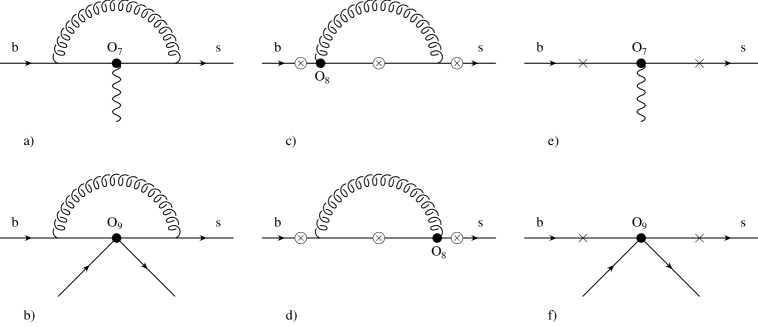
FIG. 4.: Some Feynman diagrams for $b\rightarrow s\gamma^{*}$ or $b\rightarrow s\ell^{+}\ell^{-}$ associated with the operators $O_{7}$, $O_{8}$ and $O_{9}$. The circle-crosses denote the possible locations where the virtual photon is emitted, while the crosses mark the possible locations for gluon bremsstrahlung. See text.

As the hadronic parts of the operators $O_{9}$ and $O_{10}$ are identical, the QCD corrected matrix element of $O_{10}$ can easily be obtained from the one of $O_{9}$. We therefore present only the calculation for $\langle s\ell^{+}\ell^{-}|O_{9}|b\rangle$ in some detail. The virtual corrections to this matrix element consist of the vertex correction shown in Fig. 4b) and of the quark self-energy contributions. The result can be written as

$$\langle s\ell^{+}\ell^{-}|C_{9}O_{9}|b\rangle=\widetilde{C}_{9}^{(0)}\left(-\frac{\alpha_{s}}{4\pi}\right)\left[F_{9}^{(9)}\langle\widetilde{O}_{9}\rangle_{\text{tree}}+F_{9}^{(7)}\langle\widetilde{O}_{7}\rangle_{\text{tree}}\right],$$ (94)

with $\widetilde{O}_{9}=\frac{\alpha_{s}}{4\pi}\,O_{9}$ and $\widetilde{C}_{9}^{(0)}=\frac{4\pi}{\alpha_{s}}\left(C_{9}^{(0)}+\frac{\alpha_{s}}{4\pi}C_{9}^{(1)}\right)$.

We evaluate diagram 4b) keeping the strange quark mass $m_{s}$ as a regulator of collinear singularities. The unrenormalized contributions of diagram 4b) to the form factors $F_{9}^{(7)}$ and $F_{9}^{(9)}$ read

$$F_{9}^{(9)}[4b] = -\frac{\left(\frac{\mu}{m_{b}}\right)^{2\epsilon}}{\epsilon}\frac{4}{3}+\frac{\left(\frac{\mu}{m_{b}}\right)^{2\epsilon}}{\epsilon_{\text{IR}}}\frac{8}{3}\left(\hat{s}+\frac{1}{2}\,\hat{s}^{2}+\frac{1}{3}\,\hat{s}^{3}+\frac{1}{2}\ln(r)\right)$$ (96)

$$+\frac{8}{3}\ln(r)-\frac{2}{3}\ln^{2}(r)+\frac{16}{3}+\frac{20}{3}\,\hat{s}+\frac{16}{3}\,\hat{s}^{2}+\frac{116}{27}\,\hat{s}^{3}\,,$$

$$F_{9}^{(7)}[4b] = -\frac{2}{3}\hat{s}\left(1+\frac{1}{2}\,\hat{s}+\frac{1}{3}\,\hat{s}^{2}\right)\,,$$ (97)

where we kept all terms up to $\hat{s}^{3}$. $\epsilon_{\text{IR}}$ and $r=(m_{s}^{2}/m_{b}^{2})$ regularize the infrared and collinear singularities in eq. (96).

The $b$- and $s$-quark self-energy contributions are obtained by multiplying the tree level matrix element of $O_{9}$ by the quark field renormalization factor $\delta\bar{Z}_{\psi}=\sqrt{Z_{\psi}(m_{b})Z_{\psi}(m_{s})}-1$, where the explicit form for $Z_{\psi}(m)$ (in the on-shell scheme) is given in eq. (87).

Adding the self-energy contributions and the vertex correction, we get the ultraviolet finite results

$$F_{9}^{(9)}=\frac{16}{3}+\frac{20}{3}\,\hat{s}+\frac{16}{3}\,\hat{s}^{2}+\frac{116}{27}\,\hat{s}^{3}+f_{\rm{inf}}\,,$$ (98)

$$f_{\rm{inf}}=\frac{\left(\frac{\mu}{m_{b}}\right)^{2\epsilon}}{\epsilon_{\text{IR}}}\,\frac{8}{3}\,(1+\hat{s}+\frac{1}{2}\,\hat{s}^{2}+\frac{1}{3}\,\hat{s}^{3})+\frac{4}{3}\frac{\left(\frac{\mu}{m_{b}}\right)^{2\epsilon}}{\epsilon_{\text{IR}}}\,\ln(r)+\frac{2}{3}\ln(r)-\frac{2}{3}\ln^{2}(r)\,,$$ (99)

$$F_{9}^{(7)}=-\frac{2}{3}\hat{s}\left(1+\frac{1}{2}\,\hat{s}+\frac{1}{3}\,\hat{s}^{2}\right)\,.$$ (100)

At this place, it is convenient to incorporate diagram 1f) together with its counterterms discussed in section III B.

It is easy to see that the two loops in diagram 1f) factorize into two one-loop contributions. The charm loop has the Lorentz structure of $O_{9}$ and can therefore be absorbed into a modified Wilson coefficient: The renormalized diagram 1f) is properly included by modifying $\widetilde{C}^{(0)}_{9}$ in eq. (94) as follows:

$$\widetilde{C}^{(0)}_{9}\longrightarrow\widetilde{C}^{(0,\text{mod})}_{9}=\widetilde{C}^{(0)}_{9}+\left(C_{2}^{(0)}+\frac{4}{3}C_{1}^{(0)}\right)\,H_{0}\,,$$ (101)

where the charm-loop function $H_{0}$ reads (in expanded form)

$$H_{0}=\frac{1}{2835}\left[-1260+2520\ln\!\left(\frac{\mu}{m_{c}}\right)+1008\left(\frac{\hat{s}}{4z}\right)+432\left(\frac{\hat{s}}{4z}\right)^{2}+256\left(\frac{\hat{s}}{4z}\right)^{3}\right]\,.$$ (102)

In the context of virtual corrections also the ${\mathcal{O}}(\epsilon)$-part of this loop function is needed. We neglect it here since it will drop out in combination with gluon bremsstrahlung. Note that $H_{0}=h(z,\hat{s})+8/9\,\ln(\mu/m_{b})$, with $h$ defined in [28, 41].

B Virtual corrections to the matrix element of $O_{7}$

We now turn to the virtual corrections to the matrix element of the operator $O_{7}$, consisting of the vertex- (see Fig. 4a)) and self-energy corrections. The ultraviolet singularities of the sum of these diagrams are cancelled when adding the counterterm amplitude

$$C_{7}\left[Z_{77}Z_{m_{b}}/Z_{g_{s}}^{2}-1\right]\langle s\ell^{+}\ell^{-}|O_{7}|b\rangle_{\text{tree}}\,,\quad\text{where}\quad Z_{77}=1-\frac{\alpha_{s}}{4\pi}\frac{7}{3\epsilon}\,.$$ (103)

The expressions for $Z_{m_{b}}$ and $Z_{g_{s}}$ are given in eqs. (70) and (65), respectively. The renormalized result for the contribution proportional to $C_{7}$ can be written as

$$\langle s\ell^{+}\ell^{-}|C_{7}O_{7}|b\rangle=\widetilde{C}_{7}^{(0)}\left(-\frac{\alpha_{s}}{4\pi}\right)\left[F_{7}^{(9)}\langle\widetilde{O}_{9}\rangle_{\text{tree}}+F_{7}^{(7)}\langle\widetilde{O}_{7}\rangle_{\text{tree}}\right],$$ (104)

with $\widetilde{O}_{7}=\frac{\alpha_{s}}{4\pi}\,O_{7}$ and $\widetilde{C}_{7}^{(0)}=C_{7}^{(1)}$. The expanded form factors $F_{7}^{(9)}$ and $F_{7}^{(7)}$ read

$$F_{7}^{(9)} = -\frac{16}{3}\left(1+\frac{1}{2}\,\hat{s}+\frac{1}{3}\,\hat{s}^{2}+\frac{1}{4}\,\hat{s}^{3}\right)\,,$$ (105)

$$F_{7}^{(7)} = \frac{32}{3}\,L_{\mu}+\frac{32}{3}+8\,\hat{s}+6\,\hat{s}^{2}+\frac{128}{27}\,\hat{s}^{3}+f_{\rm{inf}}\,,$$ (106)

where the infrared- and collinear singular part $f_{\rm{inf}}$ is identical to the one of $F_{9}^{(9)}$ in eq. (99). Note that the on-shell value for the renormalization factor $Z_{m_{b}}$ was used in eq. (103). Therefore, when using the expression for $F_{7}^{(7,9)}$ in the form given above, the pole mass for $m_{b}$ has to be used at lowest order.

C Virtual corrections to the matrix element of $O_{8}$

Finally, we present our results for the corrections to the matrix elements of $O_{8}$. The corresponding diagrams are shown in Fig. 4c) and d). Including the counterterm

$\displaystyle C_{8}\,\delta Z_{87}\,\langle s\ell^{+}\ell^{-}|O_{7}|b\rangle_{\text{tree}}\,,\quad\text{where}\quad\delta Z_{87}=-\frac{\alpha_{s}}{4\pi}\frac{16}{9\epsilon}\,,$yields the ultraviolet and infrared finite result

$$\langle s\ell^{+}\ell^{-}|C_{8}O_{8}|b\rangle=\widetilde{C}_{8}^{(0)}\left(-\frac{\alpha_{s}}{4\pi}\right)\left[F_{8}^{(9)}\langle\widetilde{O}_{9}\rangle_{\text{tree}}+F_{8}^{(7)}\langle\widetilde{O}_{7}\rangle_{\text{tree}}\right],$$ (107)

with $\widetilde{C}_{8}^{(0)}=C_{8}^{(1)}$. The expanded form factors $F_{8}^{(9)}$ and $F_{8}^{(7)}$ read

$$F_{8}^{(9)} = \frac{104}{9}-\frac{32}{27}\,\pi^{2}+\left(\frac{1184}{27}-\frac{40}{9}\,\pi^{2}\right)\hat{s}+\left(\frac{14212}{135}-\frac{32}{3}\,\pi^{2}\right)\hat{s}^{2}$$ (109)

$$+\left(\frac{193444}{945}-\frac{560}{27}\,\pi^{2}\right)\hat{s}^{3}+\frac{16}{9}\,L_{s}\left(1+\hat{s}+\hat{s}^{2}+\hat{s}^{3}\right)\,,$$

$$F_{8}^{(7)} = -\frac{32}{9}\,L_{\mu}+\frac{8}{27}\,\pi^{2}-\frac{44}{9}-\frac{8}{9}\,i\pi+\left(\frac{4}{3}\,\pi^{2}-\frac{40}{3}\right)\hat{s}+\left(\frac{32}{9}\,\pi^{2}-\frac{316}{9}\right)\hat{s}^{2}$$ (111)

$$+\left(\frac{200}{27}\,\pi^{2}-\frac{658}{9}\right)\hat{s}^{3}-\frac{8}{9}\,L_{s}\left(\hat{s}+\hat{s}^{2}+\hat{s}^{3}\right)\,.$$

V Bremsstrahlung corrections

First of all, we remark that in the present paper only those bremsstrahlung diagrams are taken into account which are needed to cancel the infrared and collinear singularities appearing in the virtual corrections. All the other bremsstrahlung contributions (which are finite), will be given elsewhere [44].

It is known [28, 24] that the contribution to the inclusive decay width coming from the interference between the tree-level and the one-loop matrix elements of $O_{9}$ (Fig. 4b)) and from the corresponding bremsstrahlung corrections (Fig. 4f)) can be written in the form

$$\frac{d\Gamma_{99}}{d\hat{s}} = \frac{d\Gamma_{99}^{\rm{virt}}}{d\hat{s}}+\frac{d\Gamma_{99}^{\rm{brems}}}{d\hat{s}}$$ (112)

$$\frac{d\Gamma_{99}}{d\hat{s}} = \left(\frac{\alpha_{em}}{4\pi}\right)^{2}\frac{G_{F}^{2}\,m_{b,pole}^{5}\left|V_{ts}^{*}V_{tb}\right|^{2}}{48\pi^{3}}(1-\hat{s})^{2}\left(1+2\hat{s}\right)\left[2\left|\widetilde{C}_{9}^{(0)}\right|^{2}\frac{\alpha_{s}}{\pi}\,\omega_{9}(\hat{s})\right]\,,$$ (113)

where $\widetilde{C}_{9}^{(0)}=\frac{4\pi}{\alpha_{s}}\left(C_{9}^{(0)}+\frac{\alpha_{s}}{4\pi}C_{9}^{(1)}\right)$. This procedure corresponds to encapsulating the virtual and bremsstrahlung corrections in the tree-level calculation by replacing $\langle O_{9}\rangle_{\text{tree}}$ through $\left(1+\frac{\alpha_{s}}{\pi}\,\omega_{9}(\hat{s})\right)\langle O_{9}\rangle_{\text{tree}}$. The function $\omega_{9}(\hat{s})\equiv\omega(\hat{s})$, which contains all information on virtual and bremsstrahlung corrections, can be found in [24, 28] and is given by

$$\omega_{9}(\hat{s}) = -\frac{4}{3}\mbox{Li}(\hat{s})-\frac{2}{3}\ln(1-\hat{s})\ln(\hat{s})-\frac{2}{9}\pi^{2}-\frac{5+4\hat{s}}{3(1+2\hat{s})}\ln(1-\hat{s})$$ (115)

$$-\frac{2\hat{s}(1+\hat{s})(1-2\hat{s})}{3(1-\hat{s})^{2}(1+2\hat{s})}\ln(\hat{s})+\frac{5+9\hat{s}-6\hat{s}^{2}}{6(1-\hat{s})(1+2\hat{s})}\,.$$

Replacing $\widetilde{C}_{9}^{(0)}$ by $\widetilde{C}_{9}^{(0,\text{mod})}$ (see eq. (101)) in eq. (112), diagram 1f) and the corresponding bremsstrahlung corrections are automatically included.

For the combination of the interference terms between the tree-level and the one-loop matrix element of $O_{7}$ (Fig. 4a)) and the corresponding bremsstrahlung corrections (Fig. 4e)) we make the ansatz

$$\frac{d\Gamma_{77}}{d\hat{s}} = \frac{d\Gamma_{77}^{\text{virt}}}{d\hat{s}}+\frac{d\Gamma_{77}^{\text{brems}}}{d\hat{s}}$$ (116)

$$\frac{d\Gamma_{77}}{d\hat{s}} = \left(\frac{\alpha_{em}}{4\pi}\right)^{2}\frac{G_{F}^{2}\,m_{b,pole}^{5}\left|V_{ts}^{*}V_{tb}\right|^{2}}{48\pi^{3}}(1-\hat{s})^{2}\,4\,(1+2/\hat{s})\left[2\left|\widetilde{C}_{7}^{(0)}\right|^{2}\frac{\alpha_{s}}{\pi}\,\omega_{7}(\hat{s})\right]\,,$$ (117)

where $\widetilde{C}_{7}^{(0)}=C_{7}^{(1)}$. This time, the encapsulation of virtual and bremsstrahlung corrections is provided by the replacement $\langle O_{7}\rangle_{\text{tree}}\rightarrow\left(1+\frac{\alpha_{s}}{\pi}\,\omega_{7}(\hat{s})\right)\langle O_{7}\rangle_{\text{tree}}$. In order to simplify the calculation of $\omega_{7}(\hat{s})$, we make the important observation that the form factors $F^{(7)}_{7}$ and $F^{(9)}_{9}$ have the same infrared divergent part $f_{\rm{inf}}$ (eq. (106) and (98)), whereas $F^{(9)}_{7}$ and $F^{(7)}_{9}$ are finite. Taking into account that in $d$ dimensions the decay width $d\Gamma(b\rightarrow s\ell^{+}\ell^{-})/d\hat{s}$ corresponding to the matrix element

$$M(b\rightarrow s\ell^{+}\ell^{-})=\langle s\ell^{+}\ell^{-}|\widetilde{C}_{7}^{(0)}\,\widetilde{O}_{7}^{(0)}+\widetilde{C}_{9}^{(0)}\,\widetilde{O}_{9}^{(0)}+\widetilde{C}_{10}^{(0)}\,\widetilde{O}_{10}^{(0)}|b\rangle_{\text{tree}}$$ (118)

is given by

$$\frac{d\Gamma(b\rightarrow X_{s}\ell^{+}\ell^{-})}{d\hat{s}}=\left(\frac{\alpha_{em}}{4\pi}\right)^{2}\,\frac{G_{F}^{2}m_{b,pole}^{5}\left|V_{ts}^{*}V_{tb}\right|^{2}}{48\pi^{3}}\,(1-\hat{s})^{2}\,(1+{\cal O}(d-4))\times$$ (119)

$$\left(\left(1+(d-2)\hat{s}\right)\left(\left|\widetilde{C}_{9}^{(0)}\right|^{2}+\left|\widetilde{C}_{10}^{(0)}\right|^{2}\right)+4(1+(d-2)/\hat{s})\left|\widetilde{C}_{7}^{(0)}\right|^{2}+4(d-1)\mbox{Re}\left(\widetilde{C}_{7}^{(0)}\widetilde{C}_{9}^{(0)*}\right)\right)\,,$$ (120)

one concludes that the combination

$$\Delta\Gamma^{\text{virt}}=\frac{\left|\widetilde{C}_{9}^{(0)}\right|^{-2}}{1+(d-2)\hat{s}}\frac{d\Gamma^{\text{virt}}_{99}}{d\hat{s}}-\frac{\left|\widetilde{C}_{7}^{(0)}\right|^{-2}}{4(1+(d-2)/\hat{s})}\frac{d\Gamma^{\text{virt}}_{77}}{d\hat{s}}\,,$$ (121)

is free of infrared and collinear singularities. Defining analogously

$$\Delta\Gamma^{\text{brems}}=\frac{\left|\widetilde{C}_{9}^{(0)}\right|^{-2}}{1+(d-2)\hat{s}}\frac{d\Gamma^{\text{brems}}_{99}}{d\hat{s}}-\frac{\left|\widetilde{C}_{7}^{(0)}\right|^{-2}}{4(1+(d-2)/\hat{s})}\frac{d\Gamma^{\text{brems}}_{77}}{d\hat{s}}$$ (122)

and using the identity

$$\frac{\left|\widetilde{C}_{9}^{(0)}\right|^{-2}}{1+(d-2)\hat{s}}\frac{d\Gamma_{99}}{d\hat{s}}-\frac{\left|\widetilde{C}_{7}^{(0)}\right|^{-2}}{4(1+(d-2)/\hat{s})}\frac{d\Gamma_{77}}{d\hat{s}}=\Delta\Gamma^{\text{virt}}+\Delta\Gamma^{\text{brems}}\,,$$ (123)

one concludes that also $\Delta\Gamma^{\text{brems}}$ is finite. This is because $d\Gamma_{99}/d\hat{s}$ and $d\Gamma_{77}/d\hat{s}$ are finite due to the Kinoshita-Lee-Nauenberg theorem and because $\Delta\Gamma^{\text{virt}}$ is finite as mentioned above. The calculation of $\Delta\Gamma^{\text{brems}}$ is straightforward, as the integrand, expanded in $\epsilon$, leads to unproblematic integrals. Using the explicit results for $\Delta\Gamma^{\text{virt}}$, $\Delta\Gamma^{\text{brems}}$ and $\omega_{9}(\hat{s})$, one can readily extract $\omega_{7}(\hat{s})$ from eq. (123):

$$\omega_{7}(\hat{s}) = -\frac{8}{3}\,\ln\left(\frac{\mu}{m_{b}}\right)-\frac{4}{3}\,\mbox{Li}(\hat{s})-\frac{2}{9}\,\pi^{2}-\frac{2}{3}\,\ln(\hat{s})\ln(1-\hat{s})-\frac{1}{3}\,\frac{8+\hat{s}}{2+\hat{s}}\ln(1-\hat{s})$$ (125)

$$-\frac{2}{3}\,\frac{\hat{s}\left(2-2\,\hat{s}-\hat{s}^{2}\right)}{(1-\hat{s})^{2}(2+\hat{s})}\ln(\hat{s})-\frac{1}{18}\,\frac{16-11\,\hat{s}-17\,\hat{s}^{2}}{(2+\hat{s})(1-\hat{s})}\,.$$

The reasoning for the interference terms between the tree-level matrix element of $O_{7}$ and the one-loop matrix element of $O_{9}$ and vice versa is analogous: We may combine this contribution with the corresponding bremsstrahlung terms coming from the interference of diagrams 4e) and 4f) making the ansatz

$$\frac{d\Gamma_{79}}{d\hat{s}} = \frac{d\Gamma_{79}^{\text{virt}}}{d\hat{s}}+\frac{d\Gamma_{79}^{\text{brems}}}{d\hat{s}}$$ (126)

$$\frac{d\Gamma_{79}}{d\hat{s}} = \left(\frac{\alpha_{em}}{4\pi}\right)^{2}\frac{G_{F}^{2}\,m_{b,pole}^{5}\left|V_{ts}^{*}V_{tb}\right|^{2}}{48\pi^{3}}(1-\hat{s})^{2}\,12\,\left[2\,\mbox{Re}\left(\widetilde{C}_{7}^{(0)}\widetilde{C}_{9}^{(0)*}\right)\,\frac{\alpha_{s}}{\pi}\,\omega_{79}(\hat{s})\,\right]\,.$$ (127)

The corresponding encapsulation is realized by the replacement $\langle O_{7,9}\rangle_{\text{tree}}\rightarrow\left(1+\frac{\alpha_{s}}{\pi}\omega_{79}(\hat{s})\right)\langle O_{7,9}\rangle_{\text{tree}}$. This time, we make use of the fact that the quantities

$$\Delta\Gamma^{\text{virt}}_{\text{mixed}} = \frac{\left|\widetilde{C}_{9}^{(0)}\right|^{-2}}{1+(d-2)\hat{s}}\frac{d\Gamma^{\text{virt}}_{99}}{d\hat{s}}-\frac{\mbox{Re}\left[\widetilde{C}_{7}^{(0)}\widetilde{C}_{9}^{(0)*}\right]^{-1}}{4(d-1)}\frac{d\Gamma^{\text{virt}}_{79}}{d\hat{s}}\quad\quad\quad\text{and}$$ (128)

$$\Delta\Gamma^{\text{brems}}_{\text{mixed}} = \frac{\left|\widetilde{C}_{9}^{(0)}\right|^{-2}}{1+(d-2)\hat{s}}\frac{d\Gamma^{\text{brems}}_{99}}{d\hat{s}}-\frac{\mbox{Re}\left[\widetilde{C}_{7}^{(0)}\widetilde{C}_{9}^{(0)*}\right]^{-1}}{4(d-1)}\frac{d\Gamma^{\text{brems}}_{79}}{d\hat{s}}$$ (129)

are finite. For the function $\omega_{79}(\hat{s})$ we obtain

$$\omega_{79}(\hat{s}) = -\frac{4}{3}\,\ln\left(\frac{\mu}{m_{b}}\right)-\frac{4}{3}\,\mbox{Li}(\hat{s})-\frac{2}{9}\,\pi^{2}-\frac{2}{3}\,\ln(\hat{s})\ln(1-\hat{s})-\frac{1}{9}\,\frac{2+7\hat{s}}{\hat{s}}\ln(1-\hat{s})$$ (131)

$$-\frac{2}{9}\,\frac{\hat{s}\left(3-2\,\hat{s}\right)}{\left(1-\hat{s}\right)^{2}}\ln(\hat{s})+\frac{1}{18}\,\frac{5-9\,\hat{s}}{1-\hat{s}}\,.$$

Note that the procedure described here does work only if one of the functions $\omega_{7}(\hat{s})$, $\omega_{9}(\hat{s})$ or $\omega_{79}(\hat{s})$ is known already.

Finally, we remark that the combined virtual- and bremsstrahlung corrections to the operator $O_{10}$ (which has the same hadronic structure as $O_{9}$) is described by the function $\omega_{9}(\hat{s})$, too:

$$\frac{d\Gamma_{10,10}}{d\hat{s}} = \frac{d\Gamma_{10,10}^{\rm{virt}}}{d\hat{s}}+\frac{d\Gamma_{10,10}^{\rm{brems}}}{d\hat{s}}$$ (132)

$$\frac{d\Gamma_{10,10}}{d\hat{s}} = \left(\frac{\alpha_{em}}{4\pi}\right)^{2}\frac{G_{F}^{2}\,m_{b,pole}^{5}\left|V_{ts}^{*}V_{tb}\right|^{2}}{48\pi^{3}}(1-\hat{s})^{2}\left(1+2\hat{s}\right)\left[2\left(\widetilde{C}_{10}^{(0)}\right)^{2}\frac{\alpha_{s}}{\pi}\,\omega_{9}(\hat{s})\right]\,,$$ (133)

where $\widetilde{C}_{10}^{(0)}=C_{10}^{(1)}$.

VI Corrections to the decay width for $b\rightarrow X_{s}\ell^{+}\ell^{-}$

In this chapter we combine the virtual corrections calculated in chapters III, IV and the bremsstrahlung contributions discussed in chapter V and study their influence on the decay width $d\Gamma(b\rightarrow X_{s}\ell^{+}\ell^{-})/d\hat{s}$. In the literature (see e.g. [41]), this decay width is usually written as

$$\frac{d\Gamma(b\rightarrow X_{s}\ell^{+}\ell^{-})}{d\hat{s}}=\left(\frac{\alpha_{em}}{4\pi}\right)^{2}\frac{G_{F}^{2}m_{b,pole}^{5}\left|V_{ts}^{*}V_{tb}\right|^{2}}{48\pi^{3}}(1-\hat{s})^{2}\,\times\\ \left(\left(1+2\hat{s}\right)\left(\left|\widetilde{C}_{9}^{{\text{eff}}}\right|^{2}+\left|\widetilde{C}_{10}^{{\text{eff}}}\right|^{2}\right)+4(1+2/\hat{s})\left|\widetilde{C}_{7}^{{\text{eff}}}\right|^{2}+12\,\mbox{Re}\left(\widetilde{C}_{7}^{{\text{eff}}}\widetilde{C}_{9}^{{\text{eff}}*}\right)\right)\,,$$ (134)

where the contributions calculated so far have been absorbed into the effective Wilson coefficients $\widetilde{C}_{7}^{{\text{eff}}}$, $\widetilde{C}_{9}^{{\text{eff}}}$ and $\widetilde{C}_{10}^{{\text{eff}}}$. It turns out that also the new contributions calculated in the present paper can be absorbed into these coefficients. Following as closely as possible the ’parameterization’ given recently by Bobeth et al. [41], we write

$$\widetilde{C}_{9}^{{\text{eff}}} = \left(1+\frac{\alpha_{s}(\mu)}{\pi}\omega_{9}(\hat{s})\right)\big{(}A_{9}+T_{9}\,h(z,\hat{s})+U_{9}\,h(1,\hat{s})+W_{9}\,h(0,\hat{s})\big{)}$$ (136)

$$\quad\quad\quad-\frac{\alpha_{s}(\mu)}{4\pi}\left(C_{1}^{(0)}F_{1}^{(9)}+C_{2}^{(0)}F_{2}^{(9)}+A_{8}^{(0)}F_{8}^{(9)}\right)$$

$$\widetilde{C}_{7}^{{\text{eff}}} = \left(1+\frac{\alpha_{s}(\mu)}{\pi}\omega_{7}(\hat{s})\right)A_{7}-\frac{\alpha_{s}(\mu)}{4\pi}\left(C_{1}^{(0)}F_{1}^{(7)}+C_{2}^{(0)}F_{2}^{(7)}+A_{8}^{(0)}F_{8}^{(7)}\right)$$ (137)

$$\widetilde{C}_{10}^{{\text{eff}}} = \left(1+\frac{\alpha_{s}(\mu)}{\pi}\omega_{9}(\hat{s})\right)A_{10}\,,$$ (138)

where the expressions for $h(z,\hat{s})$ and $\omega_{9}(\hat{s})$ (see eqs. (102) and (115)) were already available in the literature [24, 28, 41]. The quantities $\omega_{7}(\hat{s})$ and $F_{1,2,8}^{(7,9)}$, on the other hand, have been calculated in the present paper. We take the numerical values for $A_{7}$, $A_{9}$, $A_{10}$, $T_{9}$, $U_{9}$, and $W_{9}$ from [41], while $C_{1}^{(0)}$, $C_{2}^{(0)}$ and $A_{8}^{(0)}=\widetilde{C}_{8}^{(0,{\text{eff}})}$ can be found in [48]. For completeness we list them in Tab. III.

	$\mu=2.5$ GeV	$\mu=5$ GeV	$\mu=10$ GeV
$\alpha_{s}$	$0.267$	$0.215$	$0.180$
$C_{1}^{(0)}$	$-0.697$	$-0.487$	$-0.326$
$C_{2}^{(0)}$	$1.046$	$1.024$	$1.011$
$\big{(}A_{7}^{(0)},~{}A_{7}^{(1)}\big{)}$	$(-0.360,~{}0.031)$	$(-0.321,~{}0.019)$	$(-0.287,~{}0.008)$
$A_{8}^{(0)}$	$-0.164$	$-0.148$	$-0.134$
$\big{(}A_{9}^{(0)},~{}A_{9}^{(1)}\big{)}$	$(4.241,~{}-0.170)$	$(4.129,~{}0.013)$	$(4.131,~{}0.155)$
$\big{(}T_{9}^{((0))},~{}T_{9}^{(1)}\big{)}$	$(0.115,~{}0.278)$	$(0.374,~{}0.251)$	$(0.576,~{}0.231)$
$\big{(}U_{9}^{(0)},~{}U_{9}^{(1)}\big{)}$	$(0.045,~{}0.023)$	$(0.032,~{}0.016)$	$(0.022,~{}0.011)$
$\big{(}W_{9}^{(0)},~{}W_{9}^{(1)}\big{)}$	$(0.044,~{}0.016)$	$(0.032,~{}0.012)$	$(0.022,~{}0.009)$
$\big{(}A_{10}^{(0)},~{}A_{10}^{(1)}\big{)}$	$(-4.372,~{}0.135)$	$(-4.372,~{}0.135)$	$(-4.372,~{}0.135)$

TABLE III.: Coefficients appearing in eq. (136) for $\mu=2.5$ GeV, $\mu=5$ GeV and $\mu=10$ GeV. For $\alpha_{s}(\mu)$ (in the $\overline{\mbox{MS}}$ scheme) we used the two- loop expression with 5 flavors and $\alpha_{s}(m_{Z})=0.119$. The entries correspond to the pole top quark mass $m_{t}=174$ GeV. The superscript (0) refers to lowest order quantities while the superscript (1) denotes the correction terms of order $\alpha_{s}$.

FIG. 5.: The three solid curves illustrate the $\mu$ dependence of $\mbox{Re}\,\widetilde{C}_{7}^{{\text{eff}}}(\hat{s})$ when the new corrections are included. The dashed curves are obtained when switching off these corrections. We set $\hat{m}_{c}=0.29$. See text.

In Fig. 5 we illustrate the renormalization scale dependence of $\mbox{Re}\,\widetilde{C}_{7}^{{\text{eff}}}(\hat{s})$. The dashed curves are obtained by neglecting the corrections calculated in this paper, i.e., $\omega_{7}(\hat{s})$, $F_{1}^{(7)}$, $F_{2}^{(7)}$ and $F_{8}^{(7)}$ are put equal to zero in eq. (136). The three curves correspond to the values of the renormalization scale $\mu=2.5$ GeV (lowest), $\mu=5$ GeV (middle) and $\mu=10$ GeV (uppermost). The solid curves are obtained by taking into account the new corrections. In this case, the lowest, middle and uppermost curve correspond to $\mu=10$ GeV, 5 GeV and 2.5 GeV, respectively. We conclude that the new corrections significantly reduce the renormalization scale dependence of $\mbox{Re}\,\widetilde{C}_{7}^{{\text{eff}}}(\hat{s})$.

FIG. 6.: The three solid curves illustrate the $\mu$ dependence of $\mbox{Re}\,\widetilde{C}_{9}^{{\text{eff}}}(\hat{s})$ when the new corrections are included. The dashed curves are obtained when switching off these corrections. We set $\hat{m}_{c}=0.29$. See text.

Fig. 6 shows the renormalization scale dependence of $\mbox{Re}\,\widetilde{C}_{9}^{{\text{eff}}}(\hat{s})$. Again, the dashed curves are obtained by neglecting the new corrections in eq. (136), i.e., $F_{1}^{(9)}$, $F_{2}^{(9)}$ and $F_{8}^{(9)}$ are put to zero. We stress that $\omega_{9}(\hat{s})$ is retained, as this function has been known before. The three curves correspond to the values of the renormalization scale $\mu=2.5$ GeV (lowest), $\mu=5$ GeV (middle) and $\mu=10$ GeV (uppermost). The solid curves take the new corrections into account. Now, the lowest, middle and uppermost curve correspond to $\mu=2.5$ GeV, 5 GeV and 10 GeV, respectively. We conclude that the new corrections significantly reduce the renormalization scale dependence of $\mbox{Re}\,\widetilde{C}_{9}^{{\text{eff}}}(\hat{s})$, too.

When calculating the decay width (134), we retain only terms linear in $\alpha_{s}$ (and thus in $\omega_{7}$, $\omega_{9}$) in the expressions for $|\widetilde{C}_{7}^{{\text{eff}}}|^{2}$, $|\widetilde{C}_{9}^{{\text{eff}}}|^{2}$ and $|\widetilde{C}_{10}^{{\text{eff}}}|^{2}$. In the interference term $\mbox{Re}\left(\widetilde{C}_{7}^{{\text{eff}}}\widetilde{C}_{9}^{{\text{eff}}*}\right)$ too, we keep only linear contributions in $\alpha_{s}$. By construction, one has to make the replacements $\omega_{9}\rightarrow\omega_{79}$ and $\omega_{7}\rightarrow\omega_{79}$ in this term.

Our results include all the relevant virtual corrections and those bremsstrahlung diagrams which generate infrared and collinear singularities. There exist additional bremsstrahlung terms coming e.g. from one-loop $O_{1}$ and $O_{2}$ diagrams in which both, the virtual photon and the gluon, are emitted from the charm quark line. These contributions do not induce additional renormalization scale dependence as they are ultraviolet finite. Using our experience from $b\rightarrow s\gamma$ and $b\rightarrow sg$, these contributions are not expected to be large, but to give a definitive answer concerning their size, they have to be calculated [44].

VII Numerical results for $R_{\text{quark}}(\hat{s})$

The decay width in eq. (134) has a large uncertainty due to the factor $m_{b,pole}^{5}$. Following common practice, we consider the ratio

$$R_{\text{quark}}(\hat{s})=\frac{1}{\Gamma(b\rightarrow X_{c}e\bar{\nu})}\,\frac{d\Gamma(b\rightarrow X_{s}\ell^{+}\ell^{-})}{d\hat{s}}\,,$$ (139)

in which the factor $m_{b,pole}^{5}$ drops out. The explicit expression for the semi-leptonic decay width $\Gamma(b\rightarrow X_{c}e\nu_{e})$ reads

$$\Gamma(b\rightarrow X_{c}e\bar{\nu})=\frac{G_{F}^{2}\,m_{b,pole}^{5}}{192\pi^{3}}\,|V_{cb}|^{2}\,g\!\left(\frac{m_{c,pole}^{2}}{m_{b,pole}^{2}}\right)\,K\!\left(\frac{m_{c}^{2}}{m_{b}^{2}}\right)\,,$$ (140)

where $g(z)=1-8\,z+8\,z^{3}-z^{4}-12\,z^{2}\,\ln(z)\,$ is the phase space factor, and

$$K(z)=1-\frac{2\alpha_{s}(m_{b})}{3\pi}\,\frac{f(z)}{g(z)}$$ (141)

incorporates the next-to-leading QCD correction to the semi-leptonic decay [49]. The function $f(z)$ has been given analytically in ref. [50]:

$$f(z)=-(1-z^{2})\,\left(\frac{25}{4}-\frac{239}{3}\,z+\frac{25}{4}\,z^{2}\right)+z\,\ln(z)\left(20+90\,z-\frac{4}{3}\,z^{2}+\frac{17}{3}\,z^{3}\right)$$ (142)

$$+z^{2}\,\ln^{2}(z)\,(36+z^{2})+(1-z^{2})\,\left(\frac{17}{3}-\frac{64}{3}\,z+\frac{17}{3}\,z^{2}\right)\,\ln(1-z)$$ (143)

$$-4\,(1+30\,z^{2}+z^{4})\,\ln(z)\ln(1-z)-(1+16\,z^{2}+z^{4})\left(6\,\mbox{Li}(z)-\pi^{2}\right)$$ (144)

$$-32\,z^{3/2}(1+z)\left[\pi^{2}-4\,\mbox{Li}(\sqrt{z})+4\,\mbox{Li}(-\sqrt{z})-2\ln(z)\,\ln\left(\frac{1-\sqrt{z}}{1+\sqrt{z}}\right)\right]\,.$$ (145)

FIG. 7.: The three solid lines show the $\mu$ dependence of $R_{\text{quark}}(\hat{s})$ when including the corrections to the matrix elements calculated in this paper; the dashed lines are obtained when switching off these corrections. We set $\hat{m}_{c}=0.29$. See text.

We now turn to the numerical results for $R_{\text{quark}}(\hat{s})$ for $0.05\leq\hat{s}\leq 0.25$. In Fig. 7 we investigate the dependence of $R_{\text{quark}}(\hat{s})$ on the renormalization scale $\mu$. The solid lines are obtained by including the new NNLL contributions, as explained in chapter VI. The three solid curves correspond to $\mu=2.5$ GeV (lowest line), $\mu=5$ GeV (middle line) and $\mu=10$ GeV (uppermost line). The three dashed curves (again $\mu=2.5$ GeV for the lowest, $\mu=5$ GeV for the middle and $\mu=10$ GeV for the uppermost line), on the other hand, show the results without the new NNLL corrections, i.e., they include the NLL results combined with the NNLL corrections to the matching conditions as obtained by Bobeth et al. [41]. From this figure, we conclude that the renormalization scale dependence gets reduced by more than a factor of 2. Only for low values of $\hat{s}$ ($\hat{s}\sim 0.05$), where the NLL $\mu$-dependence is small already, the reduction factor is smaller. For the integrated quantity we obtain

$$R_{\text{quark}}=\int_{0.05}^{0.25}\,d\hat{s}\,R_{\text{quark}}(\hat{s})=(1.25\pm 0.08(\mu))\times 10^{-5}\,,$$ (146)

where the error is obtained by varying $\mu$ between 2.5 GeV and 10 GeV. Before our corrections, the result was $R_{\text{quark}}=(1.36\pm 0.18)\times 10^{-5}$ [41]. In other words, the renormalization scale dependence got reduced from $\sim\pm 13\%$ to $\sim\pm 6.5\%$.

FIG. 8.: a) $R_{\text{quark}}(\hat{s})$ for $\hat{m}_{c}=0.27$ (dashed line), $\hat{m}_{c}=0.29$ (solid line) and $\hat{m}_{c}=0.31$ (dash-dotted line) and $\mu$=5 GeV. b) $R_{\text{quark}}(\hat{s})$ for $\hat{m}_{c}=0.25$ (dashed line), $\hat{m}_{c}=0.29$ (solid line) and $\hat{m}_{c}=0.33$ (dash-dotted line) and $\mu$=5 GeV. See text.

Among the errors on $R_{\text{quark}}(\hat{s})$ which are due to the uncertainties in the input parameters, the one induced by $\hat{m}_{c}=m_{c}/m_{b}$ is known to be the largest. We repeat at this point that $m_{c}$ enters (unlike in $B\rightarrow X_{s}\gamma$) already the one-loop diagrams associated with $O_{1}$ and $O_{2}$. We did the renormalization of the charm quark mass in such a way that $m_{c}$ has the meaning of the pole mass in the one-loop expressions. The meaning of $m_{c}$ in the corresponding two-loop matrix elements, on the other hand, is not fixed (for a discussion of this issue for $B\rightarrow X_{s}\gamma$, see ref. [14]). As the running charm mass at a scale of ${\mathcal{O}}(m_{b})$ is smaller than the pole mass, it numerically makes a difference whether one inserts a pole mass- or a running mass value for $m_{c}$ in the two-loop contributions. In a thorough phenomenological analysis this issue should certainly be included when estimating the theoretical error. We decide, however, to postpone the quantitative discussion of this point and will take it up when also the finite bremsstrahlung contibutions, which complete the NNLL calculation of $R_{\text{quark}}(\hat{s})$, are available [44]. For the time being, we interpret $m_{c}$ to be the pole mass in the two-loop contributions. In Fig. 8a) we vary $\hat{m}_{c}$ between 0.27 and 0.31, while in Fig. 8b) the more conservative range $0.25\leq\hat{m}_{c}\leq 0.33$ is considered. Comparing Fig. 7 with Figs. 8a) and b), we find that at the NNLL level the uncertainty due to $\hat{m}_{c}$ is larger than the left-over $\mu$-dependence, even for the less conservative range of $\hat{m}_{c}$. For the integrated quantity $R_{\text{quark}}$ we have an uncertainty of $\pm 7.6\%$ when $\hat{m}_{c}$ is varied between 0.27 and 0.31. Varying $\hat{m}_{c}$ in the more conservative range, the corresponding uncertainty amounts to $\pm 15\%$.

A more detailed numerical analysis for $R_{\text{quark}}(\hat{s})$ and $R_{\text{quark}}$, including the errors which are due to uncertainties in other input parameters as well as non-perturbative effects, will be given in ref. [44].

To conclude: We have calculated virtual corrections of ${\mathcal{O}}(\alpha_{s})$ to the matrix elements of $O_{1}$, $O_{2}$, $O_{7}$, $O_{8}$, $O_{9}$ and $O_{10}$. We also took into account those bremsstrahlung corrections which cancel the infrared and collinear singularities in the virtual corrections. The renormalization scale dependence of $R_{\text{quark}}(\hat{s})$ gets reduced by more than a factor of 2. The calculation of the remaining bremsstrahlung contributions (which are expected to be rather small) and a more detailed numerical analysis are in progress [44].

Acknowledgements: C.G. would like to thank the members of the Yerevan Physics Institute for the kind hospitality extended to him when this paper was finalized. We thank K. Bieri and P. Liniger for helpful discussions.

A One-loop matrix elements of the four quark operators

In order to fix the counterterms $F_{i\rightarrow\rm{4quark}}^{\rm{ct}(7,9)}$ ($i=1,2$) in eq. (63), we need the one-loop matrix elements $\langle s\ell^{+}\ell^{-}|O_{j}|b\rangle_{\text{1-loop}}$ of the four-quark operators $O_{1}$, $O_{2}$, $O_{4}$, $O_{11}$ and $O_{12}$. Due to the $1/\epsilon$ factor in eq. (63), they are needed up to ${\mathcal{O}}\left(\epsilon^{1}\right)$. The explicit results (in expanded form) read

$$\langle s\ell^{+}\ell^{-}|O_{2}|b\rangle_{\text{1-loop}} = \left(\frac{\mu}{m_{c}}\right)^{2\epsilon}\,\left[\frac{4}{9\,\epsilon}+\frac{4}{2835}\left(-315+252\left(\frac{\hat{s}}{4z}\right)+108\left(\frac{\hat{s}}{4z}\right)^{2}+64\left(\frac{\hat{s}}{4z}\right)^{3}\right)\right.$$ (A1)

$$+ \left.\frac{\epsilon}{2835}\left(105\,\pi^{2}-1008\left(\frac{\hat{s}}{4z}\right)+128\left(\frac{\hat{s}}{4z}\right)^{3}\right)\right]\,\langle\widetilde{O}_{9}\rangle_{\text{tree}}\,,$$ (A2)

$$\langle s\ell^{+}\ell^{-}|O_{1}|b\rangle_{\text{1-loop}}=\frac{4}{3}\,\langle s\ell^{+}\ell^{-}|O_{2}|b\rangle_{\text{1-loop}}\,,$$ (A3)

$$\langle s\ell^{+}\ell^{-}|O_{4}|b\rangle_{\text{1-loop}} = -\left(\frac{\mu}{m_{b}}\right)^{2\epsilon}\left\{\left[\frac{4}{9}+\frac{\epsilon}{945}\left(70\,\hat{s}+7\,\hat{s}^{2}+\hat{s}^{3}\right)\right]\,\langle\widetilde{O}_{7}\rangle_{\text{tree}}\right.$$ (A4)

$$+ \left[\frac{16}{27\,\epsilon}+\frac{2}{8505}\left(-420+1260\,i\pi-1260\,L_{s}+252\,\hat{s}+27\,\hat{s}^{2}+4\,\hat{s}^{3}\right)\right.$$ (A5)

$$+ \frac{4\,\epsilon}{8505}\left(420\,i\pi+910-630\,i\,L_{s}\,\pi-420\,L_{s}-315\,\pi^{2}\right.$$ (A6)

$$+ \left.\left.\left.315\,L_{s}^{2}-126\,\hat{s}+\hat{s}^{3}\right)\right]\,\langle\widetilde{O}_{9}\rangle_{\text{tree}}\right\}\,,$$ (A7)

$$\langle s\ell^{+}\ell^{-}|O_{11}|b\rangle_{\text{1-loop}}=-\frac{64}{27}\,\left(\frac{\mu}{m_{c}}\right)^{2\epsilon}\left[1+\frac{4\,\epsilon}{5}\left({\frac{\hat{s}}{4z}}+{\frac{3}{7}}\,\left({\frac{{\hat{s}}}{{4z}}}\right)^{2}+{\frac{16}{63}}\,\left({\frac{{\hat{s}}}{{4z}}}\right)^{3}\right)\right]\,\langle\widetilde{O}_{9}\rangle_{\text{tree}}\,,$$ (A8)

$$\langle s\ell^{+}\ell^{-}|O_{12}|b\rangle_{\text{1-loop}}=\frac{3}{4}\,\langle s\ell^{+}\ell^{-}|O_{11}|b\rangle_{\text{1-loop}}\,.$$ (A9)

B Full $\hat{s}$ and ${z}$ dependence of the form factors $F^{(7,9)}_{1,2}$

In this appendix we give the dependence of $f^{(b)}_{a}$ ($a=1,2;~{}b=7,9$) (see eq. (92)) on $\hat{s}$ and $z$. We decompose them as follows:

$\displaystyle f^{(b)}_{a}=\sum_{i,j,l,m}\kappa^{(b)}_{a,ijlm}\,\hat{s}^{i}\,L^{j}_{s}\,z^{l}\,L_{c}^{m}+\sum_{i,j}\rho^{(b)}_{a,ij}\,\hat{s}^{i}\,L^{j}_{s}\,.$The quantities $\rho^{(b)}_{a,ij}$ collect the half-integer powers of $z=m_{c}^{2}/m_{b}^{2}=\hat{m}_{c}^{2}$. This way, the summation indices in the above equation run over integers only. On the following pages, we list the numerical values of $\kappa^{(b)}_{a,ijlm}$ and $\rho^{(b)}_{a,ij}$ for

$\displaystyle i=0,...,~{}3;\quad j=0,~{}1;\quad l=-3,...,~{}3\quad\text{and}\quad m=0,...,~{}4\,.$Coefficients not explicitly mentioned below vanish.
 Coefficients $\kappa^{(9)}_{1,ijlm}$ and $\rho^{(9)}_{1,ij}$ for the decomposition of $f_{1}^{(9)}$

$$\rho^{(9)}_{1,00} =3.8991\,\hat{m}_{c}^{3} \rho^{(9)}_{1,10} =-23.3946\,\hat{m}_{c}$$ (B1)

$$\rho^{(9)}_{1,20} =-140.368\,\hat{m}_{c} \rho^{(9)}_{1,30} =7.79821\,\hat{m}_{c}^{-1}-319.726\,\hat{m}_{c}$$ (B2)

$\kappa^{(9)}_{1,00lm}=\left(\begin{tabular}[]{rcl rcl rcl rcl rcl}{}\hfil&0&{}{}&{}\hfil&0&{}{}&{}\hfil&0&{}{}&{}\hfil&0&{}{}&{}\hfil&0&{}\\ {}\hfil&0&{}{}&{}\hfil&0&{}{}&{}\hfil&0&{}{}&{}\hfil&0&{}{}&{}\hfil&0&{}\\ {}\hfil&0&{}{}&{}\hfil&0&{}{}&{}\hfil&0&{}{}&{}\hfil&0&{}{}&{}\hfil&0&{}\\ $-4.61812$&$+$&$3.67166\,i${}&$5.62963$&$+$&$1.86168\,i${}&{}\hfil&0&{}{}&{}\hfil&0&{}{}&{}\hfil&0&{}\\ $14.4621$&$-$&$16.2155\,i${}&$9.59321$&$-$&$11.1701\,i${}&$-1.18519$&$-$&$7.44674\,i${}&\lx@intercol\hfil~{}$\,-0.790123$\hfil\lx@intercol~{} &{}\hfil&0&{}\\ $-16.0864$&$+$&$26.7517\,i${}&$54.2439$&$-$&$14.8935\,i${}&$-15.4074$&$-$&$29.787\,i${}&\lx@intercol\hfil~{}$\,-3.95062$\hfil\lx@intercol~{} &{}\hfil&0&{}\\ $-14.73$&$-$&$23.6892\,i${}&$-28.5761$&$+$&$34.7514\,i${}&\lx@intercol\hfil~{}$\,20.1481$\hfil\lx@intercol~{} &{}\hfil&0&{}{}&{}\hfil&0&{}\\ \end{tabular}\right)$


$\kappa^{(9)}_{1,01lm}=\left(\begin{tabular}[]{rcl rcl rcl rcl rcl}{}\hfil&0&{}{}&{}\hfil&0&{}{}&{}\hfil&0&{}{}&{}\hfil&0&{}{}&{}\hfil&0&{}\\ {}\hfil&0&{}{}&{}\hfil&0&{}{}&{}\hfil&0&{}{}&{}\hfil&0&{}{}&{}\hfil&0&{}\\ {}\hfil&0&{}{}&{}\hfil&0&{}{}&{}\hfil&0&{}{}&{}\hfil&0&{}{}&{}\hfil&0&{}\\ $-0.0493827$&$-$&$0.103427\,i${}&{}\hfil&0&{}{}&{}\hfil&0&{}{}&{}\hfil&0&{}{}&{}\hfil&0&{}\\ \lx@intercol\hfil~{}$\,-0.592593$\hfil\lx@intercol~{} &{}\hfil&0&{}{}&{}\hfil&0&{}{}&{}\hfil&0&{}{}&{}\hfil&0&{}\\ $4.95977$&$-$&$1.86168\,i${}&$-1.18519$&$-$&$7.44674\,i${}&\lx@intercol\hfil~{}$\,-2.37037$\hfil\lx@intercol~{} &{}\hfil&0&{}{}&{}\hfil&0&{}\\ $-9.20287$&$-$&$1.65483\,i${}&$-1.0535$&$+$&$9.92898\,i${}&\lx@intercol\hfil~{}$\,3.16049$\hfil\lx@intercol~{} &{}\hfil&0&{}{}&{}\hfil&0&{}\\ \end{tabular}\right)$


$\kappa^{(9)}_{1,10lm}=\left(\begin{tabular}[]{rcl rcl rcl rcl rcl}{}\hfil&0&{}{}&{}\hfil&0&{}{}&{}\hfil&0&{}{}&{}\hfil&0&{}{}&{}\hfil&0&{}\\ {}\hfil&0&{}{}&{}\hfil&0&{}{}&{}\hfil&0&{}{}&{}\hfil&0&{}{}&{}\hfil&0&{}\\ $-2.48507$&$-$&$0.186168\,i${}&{}\hfil&0&{}{}&{}\hfil&0&{}{}&{}\hfil&0&{}{}&{}\hfil&0&{}\\ $4.47441$&$-$&$0.310281\,i${}&$1.48148$&$-$&$1.86168\,i${}&{}\hfil&0&{}{}&{}\hfil&0&{}{}&{}\hfil&0&{}\\ $71.3855$&$-$&$30.7987\,i${}&$8.47677$&$-$&$33.5103\,i${}&$12.5389$&$-$&$7.44674\,i${}&\lx@intercol\hfil~{}$\,-0.790123$\hfil\lx@intercol~{} &\lx@intercol\hfil~{}$\,0.790123$\hfil\lx@intercol\\ $-18.1301$&$+$&$66.1439\,i${}&$149.596$&$-$&$67.0206\,i${}&$-49.1852$&$-$&$81.9141\,i${}&\lx@intercol\hfil~{}$\,-11.0617$\hfil\lx@intercol~{} &{}\hfil&0&{}\\ $-72.89$&$-$&$63.7828\,i${}&$-68.135$&$+$&$134.041\,i${}&\lx@intercol\hfil~{}$\,63.6049$\hfil\lx@intercol~{} &{}\hfil&0&{}{}&{}\hfil&0&{}\\ \end{tabular}\right)$


$\kappa^{(9)}_{1,11lm}=\left(\begin{tabular}[]{rcl rcl rcl rcl rcl}{}\hfil&0&{}{}&{}\hfil&0&{}{}&{}\hfil&0&{}{}&{}\hfil&0&{}{}&{}\hfil&0&{}\\ {}\hfil&0&{}{}&{}\hfil&0&{}{}&{}\hfil&0&{}{}&{}\hfil&0&{}{}&{}\hfil&0&{}\\ {}\hfil&0&{}{}&{}\hfil&0&{}{}&{}\hfil&0&{}{}&{}\hfil&0&{}{}&{}\hfil&0&{}\\ {}\hfil&0&{}{}&{}\hfil&0&{}{}&{}\hfil&0&{}{}&{}\hfil&0&{}{}&{}\hfil&0&{}\\ $-2.66667$&$-$&$1.86168\,i${}&\lx@intercol\hfil~{}$\,-1.18519$\hfil\lx@intercol~{} &{}\hfil&0&{}{}&{}\hfil&0&{}{}&{}\hfil&0&{}\\ $18.6539$&$-$&$7.44674\,i${}&$-4.74074$&$-$&$29.787\,i${}&\lx@intercol\hfil~{}$\,-9.48148$\hfil\lx@intercol~{} &{}\hfil&0&{}{}&{}\hfil&0&{}\\ $-41.6104$&$-$&$3.72337\,i${}&$-2.37037$&$+$&$44.6804\,i${}&\lx@intercol\hfil~{}$\,14.2222$\hfil\lx@intercol~{} &{}\hfil&0&{}{}&{}\hfil&0&{}\\ \end{tabular}\right)$


$\kappa^{(9)}_{1,20lm}=\left(\begin{tabular}[]{rcl rcl rcl rcl rcl}{}\hfil&0&{}{}&{}\hfil&0&{}{}&{}\hfil&0&{}{}&{}\hfil&0&{}{}&{}\hfil&0&{}\\ $-0.403158$&$-$&$0.0199466\,i${}&{}\hfil&0&{}{}&{}\hfil&0&{}{}&{}\hfil&0&{}{}&{}\hfil&0&{}\\ $-0.0613169$&$+$&$0.0620562\,i${}&{}\hfil&0&{}{}&{}\hfil&0&{}{}&{}\hfil&0&{}{}&{}\hfil&0&{}\\ $37.1282$&$-$&$1.36524\,i${}&$22.0621$&$-$&$1.86168\,i${}&\lx@intercol\hfil~{}$\,5.33333$\hfil\lx@intercol~{} &\lx@intercol\hfil~{}$\,0.790123$\hfil\lx@intercol~{} &{}\hfil&0&{}\\ $212.74$&$-$&$52.2081\,i${}&$-21.9215$&$-$&$52.1272\,i${}&$57.1724$&$-$&$7.44674\,i${}&\lx@intercol\hfil~{}$\,-2.37037$\hfil\lx@intercol~{} &\lx@intercol\hfil~{}$\,2.37037$\hfil\lx@intercol\\ $-44.6829$&$+$&$108.713\,i${}&$272.015$&$-$&$163.828\,i${}&$-119.111$&$-$&$156.382\,i${}&\lx@intercol\hfil~{}$\,-21.3333$\hfil\lx@intercol~{} &{}\hfil&0&{}\\ $-137.203$&$-$&$106.832\,i${}&$-99.437$&$+$&$330.139\,i${}&\lx@intercol\hfil~{}$\,168.889$\hfil\lx@intercol~{} &{}\hfil&0&{}{}&{}\hfil&0&{}\\ \end{tabular}\right)$


$\kappa^{(9)}_{1,21lm}=\left(\begin{tabular}[]{rcl rcl rcl rcl rcl}{}\hfil&0&{}{}&{}\hfil&0&{}{}&{}\hfil&0&{}{}&{}\hfil&0&{}{}&{}\hfil&0&{}\\ {}\hfil&0&{}{}&{}\hfil&0&{}{}&{}\hfil&0&{}{}&{}\hfil&0&{}{}&{}\hfil&0&{}\\ {}\hfil&0&{}{}&{}\hfil&0&{}{}&{}\hfil&0&{}{}&{}\hfil&0&{}{}&{}\hfil&0&{}\\ \lx@intercol\hfil~{}$\,0.0164609$\hfil\lx@intercol~{} &{}\hfil&0&{}{}&{}\hfil&0&{}{}&{}\hfil&0&{}{}&{}\hfil&0&{}\\ $-5.33333$&$-$&$3.72337\,i${}&\lx@intercol\hfil~{}$\,-2.37037$\hfil\lx@intercol~{} &{}\hfil&0&{}{}&{}\hfil&0&{}{}&{}\hfil&0&{}\\ $40.786$&$-$&$22.3402\,i${}&$-14.2222$&$-$&$67.0206\,i${}&\lx@intercol\hfil~{}$\,-21.3333$\hfil\lx@intercol~{} &{}\hfil&0&{}{}&{}\hfil&0&{}\\ \lx@intercol\hfil~{}$\,-111.356$\hfil\lx@intercol~{} &\lx@intercol\hfil~{}$\,119.148\,i$\hfil\lx@intercol~{} &\lx@intercol\hfil~{}$\,37.9259$\hfil\lx@intercol~{} &{}\hfil&0&{}{}&{}\hfil&0&{}\\ \end{tabular}\right)$


$\kappa^{(9)}_{1,30lm}=\left(\begin{tabular}[]{rcl rcl rcl rcl rcl}$-0.0759415$&$-$&$0.00295505\,i${}&{}\hfil&0&{}{}&{}\hfil&0&{}{}&{}\hfil&0&{}{}&{}\hfil&0&{}\\ $-0.00480894$&$+$&$0.00369382\,i${}&{}\hfil&0&{}{}&{}\hfil&0&{}{}&{}\hfil&0&{}{}&{}\hfil&0&{}\\ $-1.81002$&$+$&$0.0871741\,i${}&\lx@intercol\hfil~{}$\,-0.919459$\hfil\lx@intercol~{} &\lx@intercol\hfil~{}$\,-0.197531$\hfil\lx@intercol~{} &{}\hfil&0&{}{}&{}\hfil&0&{}\\ $79.7475$&$-$&$1.72206\,i${}&$57.3171$&$-$&$1.86168\,i${}&\lx@intercol\hfil~{}$\,11.2593$\hfil\lx@intercol~{} &\lx@intercol\hfil~{}$\,2.37037$\hfil\lx@intercol~{} &{}\hfil&0&{}\\ $425.579$&$-$&$76.6479\,i${}&$-68.8016$&$-$&$69.5029\,i${}&$129.357$&$-$&$7.44674\,i${}&\lx@intercol\hfil~{}$\,-5.53086$\hfil\lx@intercol~{} &\lx@intercol\hfil~{}$\,4.74074$\hfil\lx@intercol\\ $-87.8946$&$+$&$148.481\,i${}&$417.612$&$-$&$311.522\,i${}&$-227.16$&$-$&$253.189\,i${}&\lx@intercol\hfil~{}$\,-34.7654$\hfil\lx@intercol~{} &{}\hfil&0&{}\\ $-279.268$&$-$&$135.118\,i${}&$-146.853$&$+$&$652.831\,i${}&\lx@intercol\hfil~{}$\,331.259$\hfil\lx@intercol~{} &{}\hfil&0&{}{}&{}\hfil&0&{}\\ \end{tabular}\right)$


$\kappa^{(9)}_{1,31lm}=\left(\begin{tabular}[]{rcl rcl rcl rcl rcl}{}\hfil&0&{}{}&{}\hfil&0&{}{}&{}\hfil&0&{}{}&{}\hfil&0&{}{}&{}\hfil&0&{}\\ {}\hfil&0&{}{}&{}\hfil&0&{}{}&{}\hfil&0&{}{}&{}\hfil&0&{}{}&{}\hfil&0&{}\\ {}\hfil&0&{}{}&{}\hfil&0&{}{}&{}\hfil&0&{}{}&{}\hfil&0&{}{}&{}\hfil&0&{}\\ \lx@intercol\hfil~{}$\,0.0219479$\hfil\lx@intercol~{} &{}\hfil&0&{}{}&{}\hfil&0&{}{}&{}\hfil&0&{}{}&{}\hfil&0&{}\\ $-8.2963$&$-$&$5.58505\,i${}&\lx@intercol\hfil~{}$\,-3.55556$\hfil\lx@intercol~{} &{}\hfil&0&{}{}&{}\hfil&0&{}{}&{}\hfil&0&{}\\ $70.2698$&$-$&$49.6449\,i${}&$-31.6049$&$-$&$119.148\,i${}&\lx@intercol\hfil~{}$\,-37.9259$\hfil\lx@intercol~{} &{}\hfil&0&{}{}&{}\hfil&0&{}\\ $-231.893$&$+$&$18.6168\,i${}&$11.8519$&$+$&$248.225\,i${}&\lx@intercol\hfil~{}$\,79.0123$\hfil\lx@intercol~{} &{}\hfil&0&{}{}&{}\hfil&0&{}\\ \end{tabular}\right)$


 Coefficients $\kappa^{(7)}_{1,ijlm}$ and $\rho^{(7)}_{1,ij}$ for the decomposition of $f_{1}^{(7)}$

$$\rho^{(7)}_{1,00} =1.94955\,\hat{m}_{c}^{3} \rho^{(7)}_{1,10} =11.6973\,\hat{m}_{c}$$ (B3)

$$\rho^{(7)}_{1,20} =70.1839\,\hat{m}_{c} \rho^{(7)}_{1,30} =-3.8991\,\hat{m}_{c}^{-1}+159.863\,\hat{m}_{c}$$ (B4)

$\kappa^{(7)}_{1,00lm}=\left(\begin{tabular}[]{rcl rcll rcl rcl rcl}{}\hfil&0&{}{}&{}\hfil&0&{}{}&{}&0&{}{}\hfil&{}&0&{}{}\hfil&{}&0&{}\hfil\\ {}\hfil&0&{}{}&{}\hfil&0&{}{}&{}&0&{}{}\hfil&{}&0&{}{}\hfil&{}&0&{}\hfil\\ {}\hfil&0&{}{}&{}\hfil&0&{}{}&{}&0&{}{}\hfil&{}&0&{}{}\hfil&{}&0&{}\hfil\\ $-1.14266$&$-$&$0.517135\,i${}&{}\hfil&0&{}{}&{}&0&{}{}\hfil&{}&0&{}{}\hfil&{}&0&{}\hfil\\ $-2.20356$&$+$&$1.59186\,i${}&$-5.21743$&$+$&$1.86168\,i${}&$0.592593$&$+$&$3.72337\,i${}&\lx@intercol\hfil~{}$\,0.395062$\hfil\lx@intercol~{} &{}&0&{}\hfil\\ $1.86366$&$-$&$3.06235\,i${}&\lx@intercol\hfil~{}$\,-4.66347$\hfil\lx@intercol~{} &\lx@intercol\hfil~{}$\,3.72337\,i$\hfil\lx@intercol~{} &\lx@intercol\hfil~{}$\,0.395062$\hfil\lx@intercol~{} &{}&0&{}\hfil\\ $-1.21131$&$+$&$2.89595\,i${}&$2.99588$&$-$&$2.48225\,i${}&\lx@intercol\hfil~{}$\,-4.14815$\hfil\lx@intercol~{} &{}&0&{}{}\hfil&{}&0&{}\hfil\\ \end{tabular}\right)$


$\kappa^{(7)}_{1,01lm}=0$


$\kappa^{(7)}_{1,10lm}=\left(\begin{tabular}[]{rcl rcll rcl rcl rcl}{}\hfil&0&{}{}&{}\hfil&0&{}{}&{}&0&{}{}\hfil&{}&0&{}{}\hfil&{}&0&{}\hfil\\ {}\hfil&0&{}{}&{}\hfil&0&{}{}&{}&0&{}{}\hfil&{}&0&{}{}\hfil&{}&0&{}\hfil\\ {}\hfil&0&{}{}&{}\hfil&0&{}{}&{}&0&{}{}\hfil&{}&0&{}{}\hfil&{}&0&{}\hfil\\ $-2.07503$&$+$&$1.39626\,i${}&$-0.444444$&$+$&$0.930842\,i${}&{}&0&{}{}\hfil&{}&0&{}{}\hfil&{}&0&{}\hfil\\ $-25.9259$&$+$&$5.78065\,i${}&$-3.40101$&$+$&$13.0318\,i${}&$-4.4917$&$+$&$3.72337\,i${}&\lx@intercol\hfil~{}$\,0.395062$\hfil\lx@intercol~{} &\lx@intercol\hfil~{}$\,-0.395062$\hfil\lx@intercol\\ $11.4229$&$-$&$15.2375\,i${}&$-34.0806$&$+$&$11.1701\,i${}&$10.3704$&$+$&$18.6168\,i${}&\lx@intercol\hfil~{}$\,2.37037$\hfil\lx@intercol~{} &{}&0&{}\hfil\\ $11.7509$&$+$&$15.6984\,i${}&$18.9564$&$-$&$24.8225\,i${}&\lx@intercol\hfil~{}$\,-14.6173$\hfil\lx@intercol~{} &{}&0&{}{}\hfil&{}&0&{}\hfil\\ \end{tabular}\right)$


$\kappa^{(7)}_{1,11lm}=\left(\begin{tabular}[]{rcl rcll rcl rcl rcl}{}\hfil&0&{}{}&{}\hfil&0&{}{}&{}&0&{}{}\hfil&{}&0&{}{}\hfil&{}&0&{}\hfil\\ {}\hfil&0&{}{}&{}\hfil&0&{}{}&{}&0&{}{}\hfil&{}&0&{}{}\hfil&{}&0&{}\hfil\\ {}\hfil&0&{}{}&{}\hfil&0&{}{}&{}&0&{}{}\hfil&{}&0&{}{}\hfil&{}&0&{}\hfil\\ \lx@intercol\hfil~{}$\,-0.0164609$\hfil\lx@intercol~{} &{}\hfil&0&{}{}&{}&0&{}{}\hfil&{}&0&{}{}\hfil&{}&0&{}\hfil\\ $1.03704$&$+$&$0.930842\,i${}&\lx@intercol\hfil~{}$\,0.592593$\hfil\lx@intercol~{} &{}&0&{}{}\hfil&{}&0&{}{}\hfil&{}&0&{}\hfil\\ \lx@intercol\hfil~{}$\,-4.66347$\hfil\lx@intercol~{} &\lx@intercol\hfil~{}$\,7.44674\,i$\hfil\lx@intercol~{} &\lx@intercol\hfil~{}$\,2.37037$\hfil\lx@intercol~{} &{}&0&{}{}\hfil&{}&0&{}\hfil\\ $6.73754$&$+$&$1.86168\,i${}&$1.18519$&$-$&$7.44674\,i${}&\lx@intercol\hfil~{}$\,-2.37037$\hfil\lx@intercol~{} &{}&0&{}{}\hfil&{}&0&{}\hfil\\ \end{tabular}\right)$


$\kappa^{(7)}_{1,20lm}=\left(\begin{tabular}[]{rcl rcll rcl rcl rcl}{}\hfil&0&{}{}&{}\hfil&0&{}{}&{}&0&{}{}\hfil&{}&0&{}{}\hfil&{}&0&{}\hfil\\ {}\hfil&0&{}{}&{}\hfil&0&{}{}&{}&0&{}{}\hfil&{}&0&{}{}\hfil&{}&0&{}\hfil\\ \lx@intercol\hfil~{}$\,0.00555556$\hfil\lx@intercol~{} &{}\hfil&0&{}{}&{}&0&{}{}\hfil&{}&0&{}{}\hfil&{}&0&{}\hfil\\ $-19.4691$&$+$&$1.59019\,i${}&$-11.6779$&$+$&$0.930842\,i${}&\lx@intercol\hfil~{}$\,-2.96296$\hfil\lx@intercol~{} &\lx@intercol\hfil~{}$\,-0.395062$\hfil\lx@intercol~{} &{}&0&{}\hfil\\ $-90.4953$&$+$&$14.7788\,i${}&$14.9329$&$+$&$22.3402\,i${}&$-24.438$&$+$&$3.72337\,i${}&\lx@intercol\hfil~{}$\,1.18519$\hfil\lx@intercol~{} &\lx@intercol\hfil~{}$\,-1.18519$\hfil\lx@intercol\\ $23.8816$&$-$&$32.8021\,i${}&$-82.7915$&$+$&$39.0954\,i${}&$32.2963$&$+$&$44.6804\,i${}&\lx@intercol\hfil~{}$\,5.92593$\hfil\lx@intercol~{} &{}&0&{}\hfil\\ $38.1415$&$+$&$34.8683\,i${}&$38.6436$&$-$&$80.673\,i${}&\lx@intercol\hfil~{}$\,-41.5802$\hfil\lx@intercol~{} &{}&0&{}{}\hfil&{}&0&{}\hfil\\ \end{tabular}\right)$


$\kappa^{(7)}_{1,21lm}=\left(\begin{tabular}[]{rcl rcll rcl rcl rcl}{}\hfil&0&{}{}&{}\hfil&0&{}{}&{}&0&{}{}\hfil&{}&0&{}{}\hfil&{}&0&{}\hfil\\ {}\hfil&0&{}{}&{}\hfil&0&{}{}&{}&0&{}{}\hfil&{}&0&{}{}\hfil&{}&0&{}\hfil\\ {}\hfil&0&{}{}&{}\hfil&0&{}{}&{}&0&{}{}\hfil&{}&0&{}{}\hfil&{}&0&{}\hfil\\ \lx@intercol\hfil~{}$\,-0.0164609$\hfil\lx@intercol~{} &{}\hfil&0&{}{}&{}&0&{}{}\hfil&{}&0&{}{}\hfil&{}&0&{}\hfil\\ $2.37037$&$+$&$1.86168\,i${}&\lx@intercol\hfil~{}$\,1.18519$\hfil\lx@intercol~{} &{}&0&{}{}\hfil&{}&0&{}{}\hfil&{}&0&{}\hfil\\ $-13.9904$&$+$&$3.72337\,i${}&$2.37037$&$+$&$22.3402\,i${}&\lx@intercol\hfil~{}$\,7.11111$\hfil\lx@intercol~{} &{}&0&{}{}\hfil&{}&0&{}\hfil\\ $27.5428$&$+$&$3.72337\,i${}&$2.37037$&$-$&$29.787\,i${}&\lx@intercol\hfil~{}$\,-9.48148$\hfil\lx@intercol~{} &{}&0&{}{}\hfil&{}&0&{}\hfil\\ \end{tabular}\right)$


$\kappa^{(7)}_{1,30lm}=\left(\begin{tabular}[]{rcl rcll rcl rcl rcl}{}\hfil&0&{}{}&{}\hfil&0&{}{}&{}&0&{}{}\hfil&{}&0&{}{}\hfil&{}&0&{}\hfil\\ $-0.00010778$&$+$&$0.00258567\,i${}&{}\hfil&0&{}{}&{}&0&{}{}\hfil&{}&0&{}{}\hfil&{}&0&{}\hfil\\ $0.946811$&$-$&$0.0258567\,i${}&\lx@intercol\hfil~{}$\,0.488889$\hfil\lx@intercol~{} &\lx@intercol\hfil~{}$\,0.0987654$\hfil\lx@intercol~{} &{}&0&{}{}\hfil&{}&0&{}\hfil\\ $-41.9952$&$+$&$1.63673\,i${}&$-30.2091$&$+$&$0.930842\,i${}&\lx@intercol\hfil~{}$\,-6.22222$\hfil\lx@intercol~{} &\lx@intercol\hfil~{}$\,-1.18519$\hfil\lx@intercol~{} &{}&0&{}\hfil\\ $-189.354$&$+$&$25.8196\,i${}&$42.6566$&$+$&$31.0281\,i${}&$-57.765$&$+$&$3.72337\,i${}&\lx@intercol\hfil~{}$\,2.76543$\hfil\lx@intercol~{} &\lx@intercol\hfil~{}$\,-2.37037$\hfil\lx@intercol\\ $45.1784$&$-$&$52.4207\,i${}&$-145.181$&$+$&$88.7403\,i${}&$70.9136$&$+$&$81.9141\,i${}&\lx@intercol\hfil~{}$\,11.0617$\hfil\lx@intercol~{} &{}&0&{}\hfil\\ $77.3602$&$+$&$54.2499\,i${}&$58.4491$&$-$&$184.927\,i${}&\lx@intercol\hfil~{}$\,-96.0988$\hfil\lx@intercol~{} &{}&0&{}{}\hfil&{}&0&{}\hfil\\ \end{tabular}\right)$


$\kappa^{(7)}_{1,31lm}=\left(\begin{tabular}[]{rcl rcll rcl rcl rcl}{}\hfil&0&{}{}&{}\hfil&0&{}{}&{}&0&{}{}\hfil&{}&0&{}{}\hfil&{}&0&{}\hfil\\ {}\hfil&0&{}{}&{}\hfil&0&{}{}&{}&0&{}{}\hfil&{}&0&{}{}\hfil&{}&0&{}\hfil\\ {}\hfil&0&{}{}&{}\hfil&0&{}{}&{}&0&{}{}\hfil&{}&0&{}{}\hfil&{}&0&{}\hfil\\ \lx@intercol\hfil~{}$\,-0.0164609$\hfil\lx@intercol~{} &{}\hfil&0&{}{}&{}&0&{}{}\hfil&{}&0&{}{}\hfil&{}&0&{}\hfil\\ $3.85185$&$+$&$2.79253\,i${}&\lx@intercol\hfil~{}$\,1.77778$\hfil\lx@intercol~{} &{}&0&{}{}\hfil&{}&0&{}{}\hfil&{}&0&{}\hfil\\ $-27.3882$&$+$&$13.0318\,i${}&$8.2963$&$+$&$44.6804\,i${}&\lx@intercol\hfil~{}$\,14.2222$\hfil\lx@intercol~{} &{}&0&{}{}\hfil&{}&0&{}\hfil\\ $69.4495$&$+$&$1.86168\,i${}&$1.18519$&$-$&$74.4674\,i${}&\lx@intercol\hfil~{}$\,-23.7037$\hfil\lx@intercol~{} &{}&0&{}{}\hfil&{}&0&{}\hfil\\ \end{tabular}\right)$


 Coefficients $\kappa^{(9)}_{2,ijlm}$ and $\rho^{(9)}_{2,ij}$ for the decomposition of $f_{2}^{(9)}$

$$\rho^{(9)}_{2,00} =-23.3946\,\hat{m}_{c}^{3} \rho^{(9)}_{2,10} =140.368\,\hat{m}_{c}$$ (B5)

$$\rho^{(9)}_{2,20} =842.206\,\hat{m}_{c} \rho^{(9)}_{2,30} =-46.7892\,\hat{m}_{c}^{-1}+1918.36\,\hat{m}_{c}$$ (B6)

$\kappa^{(9)}_{2,00lm}=\left(\begin{tabular}[]{rcl rcl rcl rcl rcl}{}\hfil&0&{}{}&{}\hfil&0&{}{}&{}\hfil&0&{}{}&{}\hfil&0&{}{}&{}\hfil&0&{}\\ {}\hfil&0&{}{}&{}\hfil&0&{}{}&{}\hfil&0&{}{}&{}\hfil&0&{}{}&{}\hfil&0&{}\\ {}\hfil&0&{}{}&{}\hfil&0&{}{}&{}\hfil&0&{}{}&{}\hfil&0&{}{}&{}\hfil&0&{}\\ $-24.2913$&$-$&$22.0299\,i${}&$-23.1111$&$-$&$11.1701\,i${}&{}\hfil&0&{}{}&{}\hfil&0&{}{}&{}\hfil&0&{}\\ $-86.7723$&$+$&$97.2931\,i${}&$-57.5593$&$+$&$67.0206\,i${}&$7.11111$&$+$&$44.6804\,i${}&\lx@intercol\hfil~{}$\,4.74074$\hfil\lx@intercol~{} &{}\hfil&0&{}\\ $96.5187$&$-$&$160.51\,i${}&$-325.463$&$+$&$89.3609\,i${}&$92.4444$&$+$&$178.722\,i${}&\lx@intercol\hfil~{}$\,23.7037$\hfil\lx@intercol~{} &{}\hfil&0&{}\\ $88.3801$&$+$&$142.135\,i${}&$171.457$&$-$&$208.509\,i${}&\lx@intercol\hfil~{}$\,-120.889$\hfil\lx@intercol~{} &{}\hfil&0&{}{}&{}\hfil&0&{}\\ \end{tabular}\right)$


$\kappa^{(9)}_{2,01lm}=\left(\begin{tabular}[]{rcl rcl rcl rcl rcl}{}\hfil&0&{}{}&{}\hfil&0&{}{}&{}\hfil&0&{}{}&{}\hfil&0&{}{}&{}\hfil&0&{}\\ {}\hfil&0&{}{}&{}\hfil&0&{}{}&{}\hfil&0&{}{}&{}\hfil&0&{}{}&{}\hfil&0&{}\\ {}\hfil&0&{}{}&{}\hfil&0&{}{}&{}\hfil&0&{}{}&{}\hfil&0&{}{}&{}\hfil&0&{}\\ $0.296296$&$+$&$0.620562\,i${}&{}\hfil&0&{}{}&{}\hfil&0&{}{}&{}\hfil&0&{}{}&{}\hfil&0&{}\\ \lx@intercol\hfil~{}$\,3.55556$\hfil\lx@intercol~{} &{}\hfil&0&{}{}&{}\hfil&0&{}{}&{}\hfil&0&{}{}&{}\hfil&0&{}\\ $-29.7586$&$+$&$11.1701\,i${}&$7.11111$&$+$&$44.6804\,i${}&\lx@intercol\hfil~{}$\,14.2222$\hfil\lx@intercol~{} &{}\hfil&0&{}{}&{}\hfil&0&{}\\ $55.2172$&$+$&$9.92898\,i${}&$6.32099$&$-$&$59.5739\,i${}&\lx@intercol\hfil~{}$\,-18.963$\hfil\lx@intercol~{} &{}\hfil&0&{}{}&{}\hfil&0&{}\\ \end{tabular}\right)$


$\kappa^{(9)}_{2,10lm}=\left(\begin{tabular}[]{rcl rcl rcl rcl rcl}{}\hfil&0&{}{}&{}\hfil&0&{}{}&{}\hfil&0&{}{}&{}\hfil&0&{}{}&{}\hfil&0&{}\\ {}\hfil&0&{}{}&{}\hfil&0&{}{}&{}\hfil&0&{}{}&{}\hfil&0&{}{}&{}\hfil&0&{}\\ $0.8462$&$+$&$1.11701\,i${}&{}\hfil&0&{}{}&{}\hfil&0&{}{}&{}\hfil&0&{}{}&{}\hfil&0&{}\\ $-26.8464$&$+$&$1.86168\,i${}&$-8.88889$&$+$&$11.1701\,i${}&{}\hfil&0&{}{}&{}\hfil&0&{}{}&{}\hfil&0&{}\\ $-428.313$&$+$&$184.792\,i${}&$-50.8606$&$+$&$201.062\,i${}&$-75.2337$&$+$&$44.6804\,i${}&\lx@intercol\hfil~{}$\,4.74074$\hfil\lx@intercol~{} &\lx@intercol\hfil~{}$\,-4.74074$\hfil\lx@intercol\\ $108.781$&$-$&$396.864\,i${}&$-897.575$&$+$&$402.124\,i${}&$295.111$&$+$&$491.485\,i${}&\lx@intercol\hfil~{}$\,66.3704$\hfil\lx@intercol~{} &{}\hfil&0&{}\\ $437.34$&$+$&$382.697\,i${}&$408.81$&$-$&$804.248\,i${}&\lx@intercol\hfil~{}$\,-381.63$\hfil\lx@intercol~{} &{}\hfil&0&{}{}&{}\hfil&0&{}\\ \end{tabular}\right)$


$\kappa^{(9)}_{2,11lm}=\left(\begin{tabular}[]{rcl rcl rcl rcl rcl}{}\hfil&0&{}{}&{}\hfil&0&{}{}&{}\hfil&0&{}{}&{}\hfil&0&{}{}&{}\hfil&0&{}\\ {}\hfil&0&{}{}&{}\hfil&0&{}{}&{}\hfil&0&{}{}&{}\hfil&0&{}{}&{}\hfil&0&{}\\ {}\hfil&0&{}{}&{}\hfil&0&{}{}&{}\hfil&0&{}{}&{}\hfil&0&{}{}&{}\hfil&0&{}\\ {}\hfil&0&{}{}&{}\hfil&0&{}{}&{}\hfil&0&{}{}&{}\hfil&0&{}{}&{}\hfil&0&{}\\ $16.$&$+$&$11.1701\,i${}&\lx@intercol\hfil~{}$\,7.11111$\hfil\lx@intercol~{} &{}\hfil&0&{}{}&{}\hfil&0&{}{}&{}\hfil&0&{}\\ $-111.923$&$+$&$44.6804\,i${}&$28.4444$&$+$&$178.722\,i${}&\lx@intercol\hfil~{}$\,56.8889$\hfil\lx@intercol~{} &{}\hfil&0&{}{}&{}\hfil&0&{}\\ $249.663$&$+$&$22.3402\,i${}&$14.2222$&$-$&$268.083\,i${}&\lx@intercol\hfil~{}$\,-85.3333$\hfil\lx@intercol~{} &{}\hfil&0&{}{}&{}\hfil&0&{}\\ \end{tabular}\right)$


$\kappa^{(9)}_{2,20lm}=\left(\begin{tabular}[]{rcl rcl rcl rcl rcl}{}\hfil&0&{}{}&{}\hfil&0&{}{}&{}\hfil&0&{}{}&{}\hfil&0&{}{}&{}\hfil&0&{}\\ $-0.0132191$&$+$&$0.11968\,i${}&{}\hfil&0&{}{}&{}\hfil&0&{}{}&{}\hfil&0&{}{}&{}\hfil&0&{}\\ $0.367901$&$-$&$0.372337\,i${}&{}\hfil&0&{}{}&{}\hfil&0&{}{}&{}\hfil&0&{}{}&{}\hfil&0&{}\\ $-222.769$&$+$&$8.19141\,i${}&$-132.372$&$+$&$11.1701\,i${}&\lx@intercol\hfil~{}$\,-32.$\hfil\lx@intercol~{} &\lx@intercol\hfil~{}$\,-4.74074$\hfil\lx@intercol~{} &{}\hfil&0&{}\\ $-1276.44$&$+$&$313.249\,i${}&$131.529$&$+$&$312.763\,i${}&$-343.034$&$+$&$44.6804\,i${}&\lx@intercol\hfil~{}$\,14.2222$\hfil\lx@intercol~{} &\lx@intercol\hfil~{}$\,-14.2222$\hfil\lx@intercol\\ $268.098$&$-$&$652.279\,i${}&$-1632.09$&$+$&$982.969\,i${}&$714.667$&$+$&$938.289\,i${}&\lx@intercol\hfil~{}$\,128.$\hfil\lx@intercol~{} &{}\hfil&0&{}\\ $823.218$&$+$&$640.989\,i${}&$596.622$&$-$&$1980.83\,i${}&\lx@intercol\hfil~{}$\,-1013.33$\hfil\lx@intercol~{} &{}\hfil&0&{}{}&{}\hfil&0&{}\\ \end{tabular}\right)$


$\kappa^{(9)}_{2,21lm}=\left(\begin{tabular}[]{rcl rcl rcl rcl rcl}{}\hfil&0&{}{}&{}\hfil&0&{}{}&{}\hfil&0&{}{}&{}\hfil&0&{}{}&{}\hfil&0&{}\\ {}\hfil&0&{}{}&{}\hfil&0&{}{}&{}\hfil&0&{}{}&{}\hfil&0&{}{}&{}\hfil&0&{}\\ {}\hfil&0&{}{}&{}\hfil&0&{}{}&{}\hfil&0&{}{}&{}\hfil&0&{}{}&{}\hfil&0&{}\\ \lx@intercol\hfil~{}$\,-0.0987654$\hfil\lx@intercol~{} &{}\hfil&0&{}{}&{}\hfil&0&{}{}&{}\hfil&0&{}{}&{}\hfil&0&{}\\ $32.$&$+$&$22.3402\,i${}&\lx@intercol\hfil~{}$\,14.2222$\hfil\lx@intercol~{} &{}\hfil&0&{}{}&{}\hfil&0&{}{}&{}\hfil&0&{}\\ $-244.716$&$+$&$134.041\,i${}&$85.3333$&$+$&$402.124\,i${}&\lx@intercol\hfil~{}$\,128.$\hfil\lx@intercol~{} &{}\hfil&0&{}{}&{}\hfil&0&{}\\ \lx@intercol\hfil~{}$\,668.137$\hfil\lx@intercol~{} &\lx@intercol\hfil~{}$\,-714.887\,i$\hfil\lx@intercol~{} &\lx@intercol\hfil~{}$\,-227.556$\hfil\lx@intercol~{} &{}\hfil&0&{}{}&{}\hfil&0&{}\\ \end{tabular}\right)$


$\kappa^{(9)}_{2,30lm}=\left(\begin{tabular}[]{rcl rcl rcl rcl rcl}$-0.0142243$&$+$&$0.0177303\,i${}&{}\hfil&0&{}{}&{}\hfil&0&{}{}&{}\hfil&0&{}{}&{}\hfil&0&{}\\ $0.0288536$&$-$&$0.0221629\,i${}&{}\hfil&0&{}{}&{}\hfil&0&{}{}&{}\hfil&0&{}{}&{}\hfil&0&{}\\ $10.8601$&$-$&$0.523045\,i${}&\lx@intercol\hfil~{}$\,5.51675$\hfil\lx@intercol~{} &\lx@intercol\hfil~{}$\,1.18519$\hfil\lx@intercol~{} &{}\hfil&0&{}{}&{}\hfil&0&{}\\ $-478.485$&$+$&$10.3323\,i${}&$-343.902$&$+$&$11.1701\,i${}&\lx@intercol\hfil~{}$\,-67.5556$\hfil\lx@intercol~{} &\lx@intercol\hfil~{}$\,-14.2222$\hfil\lx@intercol~{} &{}\hfil&0&{}\\ $-2553.47$&$+$&$459.887\,i${}&$412.809$&$+$&$417.017\,i${}&$-776.143$&$+$&$44.6804\,i${}&\lx@intercol\hfil~{}$\,33.1852$\hfil\lx@intercol~{} &\lx@intercol\hfil~{}$\,-28.4444$\hfil\lx@intercol\\ $527.368$&$-$&$890.889\,i${}&$-2505.67$&$+$&$1869.13\,i${}&$1362.96$&$+$&$1519.13\,i${}&\lx@intercol\hfil~{}$\,208.593$\hfil\lx@intercol~{} &{}\hfil&0&{}\\ $1675.61$&$+$&$810.709\,i${}&$881.117$&$-$&$3916.98\,i${}&\lx@intercol\hfil~{}$\,-1987.56$\hfil\lx@intercol~{} &{}\hfil&0&{}{}&{}\hfil&0&{}\\ \end{tabular}\right)$


$\kappa^{(9)}_{2,31lm}=\left(\begin{tabular}[]{rcl rcl rcl rcl rcl}{}\hfil&0&{}{}&{}\hfil&0&{}{}&{}\hfil&0&{}{}&{}\hfil&0&{}{}&{}\hfil&0&{}\\ {}\hfil&0&{}{}&{}\hfil&0&{}{}&{}\hfil&0&{}{}&{}\hfil&0&{}{}&{}\hfil&0&{}\\ {}\hfil&0&{}{}&{}\hfil&0&{}{}&{}\hfil&0&{}{}&{}\hfil&0&{}{}&{}\hfil&0&{}\\ \lx@intercol\hfil~{}$\,-0.131687$\hfil\lx@intercol~{} &{}\hfil&0&{}{}&{}\hfil&0&{}{}&{}\hfil&0&{}{}&{}\hfil&0&{}\\ $49.7778$&$+$&$33.5103\,i${}&\lx@intercol\hfil~{}$\,21.3333$\hfil\lx@intercol~{} &{}\hfil&0&{}{}&{}\hfil&0&{}{}&{}\hfil&0&{}\\ $-421.619$&$+$&$297.87\,i${}&$189.63$&$+$&$714.887\,i${}&\lx@intercol\hfil~{}$\,227.556$\hfil\lx@intercol~{} &{}\hfil&0&{}{}&{}\hfil&0&{}\\ $1391.36$&$-$&$111.701\,i${}&$-71.1111$&$-$&$1489.35\,i${}&\lx@intercol\hfil~{}$\,-474.074$\hfil\lx@intercol~{} &{}\hfil&0&{}{}&{}\hfil&0&{}\\ \end{tabular}\right)$


 Coefficients $\kappa^{(7)}_{2,ijlm}$ and $\rho^{(7)}_{2,ij}$ for the decomposition of $f_{2}^{(7)}$

$$\rho^{(7)}_{2,00}= -11.6973\,\hat{m}_{c}^{3} \rho^{(7)}_{2,10}= -70.1839\,\hat{m}_{c}$$ (B7)

$$\rho^{(7)}_{2,20}= -421.103\,\hat{m}_{c} \rho^{(7)}_{2,30}= 23.3946\,\hat{m}_{c}^{-1}-959.179\,\hat{m}_{c}$$ (B8)

$\kappa^{(7)}_{2,00lm}=\left(\begin{tabular}[]{rcl rcl rcl rcl rcl}{}\hfil&0&{}{}&{}\hfil&0&{}{}&{}\hfil&0&{}{}&{}\hfil&0&{}{}&{}\hfil&0&{}\\ {}\hfil&0&{}{}&{}\hfil&0&{}{}&{}\hfil&0&{}{}&{}\hfil&0&{}{}&{}\hfil&0&{}\\ {}\hfil&0&{}{}&{}\hfil&0&{}{}&{}\hfil&0&{}{}&{}\hfil&0&{}{}&{}\hfil&0&{}\\ $6.85597$&$+$&$3.10281\,i${}&{}\hfil&0&{}{}&{}\hfil&0&{}{}&{}\hfil&0&{}{}&{}\hfil&0&{}\\ $13.2214$&$-$&$9.55118\,i${}&$31.3046$&$-$&$11.1701\,i${}&$-3.55556$&$-$&$22.3402\,i${}&\lx@intercol\hfil~{}$\,-2.37037$\hfil\lx@intercol~{} &{}\hfil&0&{}\\ $-11.182$&$+$&$18.3741\,i${}&\lx@intercol\hfil~{}$\,27.9808$\hfil\lx@intercol~{} &\lx@intercol\hfil~{}$\,-22.3402\,i$\hfil\lx@intercol~{} &\lx@intercol\hfil~{}$\,-2.37037$\hfil\lx@intercol~{} &{}\hfil&0&{}\\ $7.26787$&$-$&$17.3757\,i${}&$-17.9753$&$+$&$14.8935\,i${}&\lx@intercol\hfil~{}$\,24.8889$\hfil\lx@intercol~{} &{}\hfil&0&{}{}&{}\hfil&0&{}\\ \end{tabular}\right)$


$\kappa^{(7)}_{2,01lm}=0$


$\kappa^{(7)}_{2,10lm}=\left(\begin{tabular}[]{rcl rcl rcl rcl rcl}{}\hfil&0&{}{}&{}\hfil&0&{}{}&{}\hfil&0&{}{}&{}\hfil&0&{}{}&{}\hfil&0&{}\\ {}\hfil&0&{}{}&{}\hfil&0&{}{}&{}\hfil&0&{}{}&{}\hfil&0&{}{}&{}\hfil&0&{}\\ {}\hfil&0&{}{}&{}\hfil&0&{}{}&{}\hfil&0&{}{}&{}\hfil&0&{}{}&{}\hfil&0&{}\\ $12.4502$&$-$&$8.37758\,i${}&$2.66667$&$-$&$5.58505\,i${}&{}\hfil&0&{}{}&{}\hfil&0&{}{}&{}\hfil&0&{}\\ $155.555$&$-$&$34.6839\,i${}&$20.4061$&$-$&$78.1908\,i${}&$26.9502$&$-$&$22.3402\,i${}&\lx@intercol\hfil~{}$\,-2.37037$\hfil\lx@intercol~{} &\lx@intercol\hfil~{}$\,2.37037$\hfil\lx@intercol\\ $-68.5374$&$+$&$91.4251\,i${}&$204.484$&$-$&$67.0206\,i${}&$-62.2222$&$-$&$111.701\,i${}&\lx@intercol\hfil~{}$\,-14.2222$\hfil\lx@intercol~{} &{}\hfil&0&{}\\ $-70.5057$&$-$&$94.1903\,i${}&$-113.738$&$+$&$148.935\,i${}&\lx@intercol\hfil~{}$\,87.7037$\hfil\lx@intercol~{} &{}\hfil&0&{}{}&{}\hfil&0&{}\\ \end{tabular}\right)$


$\kappa^{(7)}_{2,11lm}=\left(\begin{tabular}[]{rcl rcl rcl rcl rcl}{}\hfil&0&{}{}&{}\hfil&0&{}{}&{}\hfil&0&{}{}&{}\hfil&0&{}{}&{}\hfil&0&{}\\ {}\hfil&0&{}{}&{}\hfil&0&{}{}&{}\hfil&0&{}{}&{}\hfil&0&{}{}&{}\hfil&0&{}\\ {}\hfil&0&{}{}&{}\hfil&0&{}{}&{}\hfil&0&{}{}&{}\hfil&0&{}{}&{}\hfil&0&{}\\ \lx@intercol\hfil~{}$\,0.0987654$\hfil\lx@intercol~{} &{}\hfil&0&{}{}&{}\hfil&0&{}{}&{}\hfil&0&{}{}&{}\hfil&0&{}\\ $-6.22222$&$-$&$5.58505\,i${}&\lx@intercol\hfil~{}$\,-3.55556$\hfil\lx@intercol~{} &{}\hfil&0&{}{}&{}\hfil&0&{}{}&{}\hfil&0&{}\\ \lx@intercol\hfil~{}$\,27.9808$\hfil\lx@intercol~{} &\lx@intercol\hfil~{}$\,-44.6804\,i$\hfil\lx@intercol~{} &\lx@intercol\hfil~{}$\,-14.2222$\hfil\lx@intercol~{} &{}\hfil&0&{}{}&{}\hfil&0&{}\\ $-40.4253$&$-$&$11.1701\,i${}&$-7.11111$&$+$&$44.6804\,i${}&\lx@intercol\hfil~{}$\,14.2222$\hfil\lx@intercol~{} &{}\hfil&0&{}{}&{}\hfil&0&{}\\ \end{tabular}\right)$


$\kappa^{(7)}_{2,20lm}=\left(\begin{tabular}[]{rcl rcl rcl rcl rcl}{}\hfil&0&{}{}&{}\hfil&0&{}{}&{}\hfil&0&{}{}&{}\hfil&0&{}{}&{}\hfil&0&{}\\ {}\hfil&0&{}{}&{}\hfil&0&{}{}&{}\hfil&0&{}{}&{}\hfil&0&{}{}&{}\hfil&0&{}\\ \lx@intercol\hfil~{}$\,-0.0333333$\hfil\lx@intercol~{} &{}\hfil&0&{}{}&{}\hfil&0&{}{}&{}\hfil&0&{}{}&{}\hfil&0&{}\\ $116.815$&$-$&$9.54113\,i${}&$70.0677$&$-$&$5.58505\,i${}&\lx@intercol\hfil~{}$\,17.7778$\hfil\lx@intercol~{} &\lx@intercol\hfil~{}$\,2.37037$\hfil\lx@intercol~{} &{}\hfil&0&{}\\ $542.972$&$-$&$88.6728\,i${}&$-89.5971$&$-$&$134.041\,i${}&$146.628$&$-$&$22.3402\,i${}&\lx@intercol\hfil~{}$\,-7.11111$\hfil\lx@intercol~{} &\lx@intercol\hfil~{}$\,7.11111$\hfil\lx@intercol\\ $-143.29$&$+$&$196.813\,i${}&$496.749$&$-$&$234.572\,i${}&$-193.778$&$-$&$268.083\,i${}&\lx@intercol\hfil~{}$\,-35.5556$\hfil\lx@intercol~{} &{}\hfil&0&{}\\ $-228.849$&$-$&$209.21\,i${}&$-231.862$&$+$&$484.038\,i${}&\lx@intercol\hfil~{}$\,249.481$\hfil\lx@intercol~{} &{}\hfil&0&{}{}&{}\hfil&0&{}\\ \end{tabular}\right)$


$\kappa^{(7)}_{2,21lm}=\left(\begin{tabular}[]{rcl rcl rcl rcl rcl}{}\hfil&0&{}{}&{}\hfil&0&{}{}&{}\hfil&0&{}{}&{}\hfil&0&{}{}&{}\hfil&0&{}\\ {}\hfil&0&{}{}&{}\hfil&0&{}{}&{}\hfil&0&{}{}&{}\hfil&0&{}{}&{}\hfil&0&{}\\ {}\hfil&0&{}{}&{}\hfil&0&{}{}&{}\hfil&0&{}{}&{}\hfil&0&{}{}&{}\hfil&0&{}\\ \lx@intercol\hfil~{}$\,0.0987654$\hfil\lx@intercol~{} &{}\hfil&0&{}{}&{}\hfil&0&{}{}&{}\hfil&0&{}{}&{}\hfil&0&{}\\ $-14.2222$&$-$&$11.1701\,i${}&\lx@intercol\hfil~{}$\,-7.11111$\hfil\lx@intercol~{} &{}\hfil&0&{}{}&{}\hfil&0&{}{}&{}\hfil&0&{}\\ $83.9424$&$-$&$22.3402\,i${}&$-14.2222$&$-$&$134.041\,i${}&\lx@intercol\hfil~{}$\,-42.6667$\hfil\lx@intercol~{} &{}\hfil&0&{}{}&{}\hfil&0&{}\\ $-165.257$&$-$&$22.3402\,i${}&$-14.2222$&$+$&$178.722\,i${}&\lx@intercol\hfil~{}$\,56.8889$\hfil\lx@intercol~{} &{}\hfil&0&{}{}&{}\hfil&0&{}\\ \end{tabular}\right)$


$\kappa^{(7)}_{2,30lm}=\left(\begin{tabular}[]{rcl rcl rcl rcl rcl}{}\hfil&0&{}{}&{}\hfil&0&{}{}&{}\hfil&0&{}{}&{}\hfil&0&{}{}&{}\hfil&0&{}\\ $0.000646678$&$-$&$0.015514\,i${}&{}\hfil&0&{}{}&{}\hfil&0&{}{}&{}\hfil&0&{}{}&{}\hfil&0&{}\\ $-5.68087$&$+$&$0.15514\,i${}&\lx@intercol\hfil~{}$\,-2.93333$\hfil\lx@intercol~{} &\lx@intercol\hfil~{}$\,-0.592593$\hfil\lx@intercol~{} &{}\hfil&0&{}{}&{}\hfil&0&{}\\ $251.971$&$-$&$9.82039\,i${}&$181.255$&$-$&$5.58505\,i${}&\lx@intercol\hfil~{}$\,37.3333$\hfil\lx@intercol~{} &\lx@intercol\hfil~{}$\,7.11111$\hfil\lx@intercol~{} &{}\hfil&0&{}\\ $1136.13$&$-$&$154.918\,i${}&$-255.94$&$-$&$186.168\,i${}&$346.59$&$-$&$22.3402\,i${}&\lx@intercol\hfil~{}$\,-16.5926$\hfil\lx@intercol~{} &\lx@intercol\hfil~{}$\,14.2222$\hfil\lx@intercol\\ $-271.07$&$+$&$314.524\,i${}&$871.089$&$-$&$532.442\,i${}&$-425.481$&$-$&$491.485\,i${}&\lx@intercol\hfil~{}$\,-66.3704$\hfil\lx@intercol~{} &{}\hfil&0&{}\\ $-464.161$&$-$&$325.499\,i${}&$-350.695$&$+$&$1109.56\,i${}&\lx@intercol\hfil~{}$\,576.593$\hfil\lx@intercol~{} &{}\hfil&0&{}{}&{}\hfil&0&{}\\ \end{tabular}\right)$


$\kappa^{(7)}_{2,31lm}=\left(\begin{tabular}[]{rcl rcl rcl rcl rcl}{}\hfil&0&{}{}&{}\hfil&0&{}{}&{}\hfil&0&{}{}&{}\hfil&0&{}{}&{}\hfil&0&{}\\ {}\hfil&0&{}{}&{}\hfil&0&{}{}&{}\hfil&0&{}{}&{}\hfil&0&{}{}&{}\hfil&0&{}\\ {}\hfil&0&{}{}&{}\hfil&0&{}{}&{}\hfil&0&{}{}&{}\hfil&0&{}{}&{}\hfil&0&{}\\ \lx@intercol\hfil~{}$\,0.0987654$\hfil\lx@intercol~{} &{}\hfil&0&{}{}&{}\hfil&0&{}{}&{}\hfil&0&{}{}&{}\hfil&0&{}\\ $-23.1111$&$-$&$16.7552\,i${}&\lx@intercol\hfil~{}$\,-10.6667$\hfil\lx@intercol~{} &{}\hfil&0&{}{}&{}\hfil&0&{}{}&{}\hfil&0&{}\\ $164.329$&$-$&$78.1908\,i${}&$-49.7778$&$-$&$268.083\,i${}&\lx@intercol\hfil~{}$\,-85.3333$\hfil\lx@intercol~{} &{}\hfil&0&{}{}&{}\hfil&0&{}\\ $-416.697$&$-$&$11.1701\,i${}&$-7.11111$&$+$&$446.804\,i${}&\lx@intercol\hfil~{}$\,142.222$\hfil\lx@intercol~{} &{}\hfil&0&{}{}&{}\hfil&0&{}\\ \end{tabular}\right)$

REFERENCES

- [1] R. Ammar et al. (CLEO Collaboration), Phys. Rev. Lett. 71, 674 (1993).
-
[2]
M. S. Alam et al. (CLEO Collaboration),
Phys. Rev. Lett. 74, 2885 (1995);
T. E. Coan et al. (CLEO Collaboration), Report CLNS 00/1697, CLEO 00-21. -
[3]
I. Bigi et al., Phys. Rev. Lett. 71, 496 (1993);
A. Manohar and M.B. Wise, Phys. Rev. D49, 1310 (1994);
B. Blok et al., Phys. Rev. D49, 3356 (1994);
T. Mannel, Nucl. Phys. B413, 396 (1994);
A. Falk, M. Luke, and M. Savage, Phys. Rev. D49, 3367 (1994). - [4] I. Bigi et al., Phys. Lett. B293, 430 (1992); B297(E), 477 (1993).
- [5] S. Chen et al. (CLEO Collaboration), hep-ex/0108032.
- [6] R. Barate et al. (ALEPH collaboration), Phys. Lett. B429, 169 (1998).
- [7] A. Abashian et al. (BELLE collaboration), BELLE-CONF-0003.
-
[8]
A. Ali and C. Greub, Zeit. f. Phys. C49, 431 (1991);
Phys. Lett. B259, 182 (1991);
Phys. Lett. B361, 146 (1995).
A.L. Kagan and M. Neubert, Eur. Phys. J C7, 5 (1999). -
[9]
K. Adel and Y. P. Yao,
Phys. Rev. D 49, 4945 (1994);
C. Greub and T. Hurth Phys. Rev. D 56, 2934 (1997);
A. J. Buras, A. Kwiatkowski and N. Pott, Nucl. Phys. B 517, 353 (1998). - [10] M. Ciuchini, G. Degrassi, P. Gambino and G.F. Giudice, Nucl. Phys. B 527, 21 (1998).
- [11] K. Chetyrkin, M. Misiak and M. Münz, Phys. Lett. B 400, 206 (1997).
- [12] C. Greub, T. Hurth and D. Wyler, Phys. Rev. D 54, 3350 (1996).
- [13] A. J. Buras, A. Czarnecki, M. Misiak, J. Urban, hep-ph/0105160.
- [14] P. Gambino and M. Misiak, Nucl. Phys. B 611, 338 (2001).
- [15] F. Borzumati and C. Greub, Phys. Rev. D 58, 074004 (1998); Phys. Rev. D 59, 057501 (1999).
- [16] H. H. Asatryan, H. M. Asatrian, G. K. Yeghiyan and G. K. Savvidy, Int. J. Mod. Phys. A16 (2001) 3805.
- [17] S. Bertolini, F. Borzumati, A. Masiero and G. Ridolfi, Nucl. Phys. B 353, 591 (1991).
- [18] M. Ciuchini, G. Degrassi, P. Gambino and G.F. Giudice, Nucl. Phys. B 534, 3 (1998).
- [19] C. Bobeth, M. Misiak and J. Urban, Nucl. Phys. B 567, 153 (2000).
- [20] F. Borzumati, C. Greub, T. Hurth and D. Wyler, Phys. Rev. D 62, 075005 (2000).
- [21] T. Besmer, C. Greub and T. Hurth, Nucl. Phys. B 609, 359 (2001).
- [22] H. H. Asatrian and H. M. Asatrian, Phys. Lett. B460 (1999) 148.
- [23] B. Grinstein, M. J. Savage and M. B. Wise, Nucl. Phys. B 319, 271 (1989).
- [24] M. Misiak, Nucl. Phys. B393 23 (1993); E:B439 461 1995.
- [25] A. Ali, G. F. Guidice, T. Mannel, Z. Phys. C67, 417 (1995).
-
[26]
N. Desphande, J. Trampetic, K. Pancrose,
Phys. Rev. D 39, 1461 (1989);
C. S. Lim, T. Morozumi, A. I. Sanda, Phys. Lett. B 218, 343 (1989). - [27] P. Cho, M. Misiak, D. Wyler, Phys. Rev. D 54, 3329 (1996).
- [28] A. J. Buras and M. Münz, Phys. Rev. D 52, 186 (1995).
- [29] S. Glenn et al. [CLEO Collaboration], Phys. Rev. Lett. 80, 2289 (1998).
- [30] K. Abe et al. [BELLE Collaboration], BELLE-CONF-0110, hep-ex/0107072.
- [31] Z. Ligeti and M. B. Wise, Phys. Rev. D 53, 4937 (1996).
- [32] A. F. Falk, M. Luke and M. J. Savage, Phys. Rev. D 49, 3367 (1994).
- [33] A. Ali, G. Hiller, L. T. Handoko and T. Morozumi, Phys. Rev. D 55, 4105 (1997).
- [34] J-W. Chen, G. Rupak and M. J. Savage, Phys. Lett. B 410, 285 (1997).
- [35] G. Buchalla, G. Isidori and S. J. Rey, Nucl. Phys. B 511, 594 (1998).
- [36] G. Buchalla and G. Isidori, Nucl. Phys. B 525, 333 (1998).
- [37] F. Krüger and L.M. Sehgal, Phys. Lett. B 380, 199 (1996).
- [38] A. Ali, P. Ball, L.T. Handoko, G. Hiller, Phys. Rev. D 61, 074024 (2000).
- [39] E. Lunghi and I. Scimemi, Nucl. Phys. B 574, 43 (2000).
- [40] E. Lunghi, A. Masiero, I. Scimemi and L. Silvestrini, Nucl. Phys. B 568, 120 (2000).
- [41] C. Bobeth, M. Misiak and J. Urban, Nucl. Phys. B 574, 291 (2000).
- [42] H. H. Asatryan, H. M. Asatrian, C. Greub and M. Walker, Phys. Lett. B 507, 162 (2001) [hep-ph/0103087].
- [43] G. Buchalla and A. J. Buras, Nucl. Phys. B 548, 309 (1999).
- [44] H. H. Asatryan, H. M. Asatrian, C. Greub and M. Walker, in preparation.
- [45] V.A. Smirnov, Renormalization and Asymptotic Expansions, Birkhäuser, Basel, 1991.
- [46] V.A. Smirnov, Mod. Phys. Lett. A 10, 1485 (1995) [hep-th/9412063].
- [47] H. Simma and D. Wyler, Nucl. Phys. B 344, 283 (1990).
- [48] C. Greub and P. Liniger, Phys. Lett. B 494, 237 (2000); Phys. Rev. D 63, 054025 (2001).
- [49] N. Cabibbo and L. Maiani, Phys. Lett. B 79, 109 (1978).
- [50] Y. Nir, Phys. Lett. B 221, 184 (1989).