Abstract

The study of Deeply Virtual Compton Scattering has shown that electromagnetic gauge invariance requires, to leading order, not only twist two but additional twist three contributions. We apply this analysis and, using the Ellis-Furmanski-Petronzio factorization scheme, compute the single (electron) spin asymmetry arising in the collision of longitudinally polarized electrons with hadrons up to twist 3 accuracy. In order to simplify the kinematics we restrict the actual calculation to pions in the chiral limit. The process is described in terms of the generalized parton distribution functions which we obtain within a bag model framework.

1 Introduction.

Hard reactions provide important information for unveiling the structure of hadrons. The large virtuality, $Q^{2}$, involved in these processes allows the factorization of the hard (perturbative) and soft (nonperturbative) contributions in their amplitudes. Therefore these reactions are receiving great attention by the hadronic physics community. Among the hard processes one, which merits to be singled out, is the Deeply Virtual Compton Scattering (DVCS) because it can be expressed, in the asymptotic regime, in terms of the so called Generalized Parton Distributions (GPDs) [1, 2, 3]. The GPDs describe non-forward matrix elements of light-cone operators and therefore measure the response of the internal structure of the hadrons to the probes. Moreover DVSC is instrumental in the experimental interpretation of the angular momentum sum rule [4].

It has been shown that the implementation of gauge invariance in the analysis of the DVCS amplitude in the asymptotic regime, i.e. large virtuality of the incoming photon, requires the inclusion of twist-3 contributions [5]-[13]. Let us explain the reason in a brief manner. In leading twist, in the Bjorken limit, the Lorentz structure of the hard subgraph of the DVCS amplitude’s leading diagram has, at large $Q^{2}$, the form of a transverse projector. The virtual photon momentum in the form of the Sudakov decomposition contains a transverse component too. Thus their contraction does not vanish and electromagnetic gauge invariance is violated. To restore it, next-to-leading order terms in the asymptotic expansion to the DVCS amplitude, which are proportional to the transverse component of the momentum transfer, have to be included. These terms, which are twist-3, give rise to the dominant contribution in some observables. One of them is the single spin asymmetry (SSA), which arises in the collision of longitudinally polarized electrons with hadrons, and which we will analyze in here .

In this first paper we deal with a spin zero massless target, the pion. The same procedure could be applied to the scattering off unpolarized nucleons. However this calculation would require keeping the mass terms of the nucleon, a complication which we want to avoid at present [16]. Moreover, in the case of polarized nucleons, one could study besides the SSA other asymmetries, however the complexity of the analysis, with the existence of many different GPDs, is postponed for a future publication [16]. In order to calculate the twist-2 and twist-3 GPDs contributing to the SSA, a crucial ingredient of the calculation, we use an MIT bag model scheme with boosted wave functions.

The plan of our paper is as follows. In section 2 we describe the kinematics and introduce the appropriate notations. The DVCS amplitude for the pion, including up to twist-3 contributions, is presented in section 3. We follow the description of Ref.[6], where, using a generalization of the Ellis-Furmanski-Petronzio (EFP) factorization scheme [17], the complete gauge invariant DVCS amplitude has been obtained. In section 4 we outline the basic ingredients of our approach and calculate all the parametrizing functions (GPDs). Then in section 5 we give the numerical estimates of the SSA parameter for the case under study and discuss our results.

2 $eh\to\gamma eh$ process: kinematics and notations.

Our starting point is electron-hadron scattering into real photon, electron and hadron,

$$e(k)+\pi(p)\to\gamma(q^{\prime})+e(k^{\prime})+\pi(p^{\prime}),$$ (1)

assuming that the electron is longitudinally polarized. We will consider the electron to be massless,

$$k^{2}=k^{\prime\,2}=0,$$ (2)

and, that the hadron is a pion, which we take also to be massless (chiral limit),

$$p^{2}=p^{\prime\,2}=m_{\pi}^{2}\to 0.$$ (3)

In QED, to lowest order, the reaction (1) takes place via the Bethe-Heitler process, where the final real photon is emitted by one of the electrons, and the virtual Compton process

$$\gamma^{*}(q)+\pi(p)\to\gamma(q^{\prime})+\pi(p^{\prime}),$$ (4)

which becomes the DVCS process if the square of virtual photon momentum $q=k-k^{\prime}$ is very large, i.e.

$$Q^{2}=-q^{2}\to\infty.$$ (5)

For the Bethe-Heitler process the amplitude is given by

$$T_{(BH)}=-e^{3}\bar{u}(k^{\prime})\biggl{\{}\hat{\varepsilon}^{*}\frac{\hat{k}-\hat{\Delta}}{(k-\Delta)^{2}}\gamma_{\mu}+\gamma_{\mu}\frac{\hat{k}^{\prime}+\hat{\Delta}}{(k^{\prime}+\Delta)^{2}}\hat{\varepsilon}^{*}\biggr{\}}u(k)\frac{1}{\Delta^{2}}\Gamma_{\mu}(p,p^{\prime}),$$ (6)

where

$$\Delta=p^{\prime}-p,$$ (7)

and the electromagnetic vertex of the pions takes the standard form

$$\Gamma_{\mu}(p,p^{\prime})=(p+p^{\prime})_{\mu}F_{+}(\Delta^{2}).$$ (8)

$F_{+}(\Delta^{2})$ is the electromagnetic form factor of the pion. The Virtual Compton process amplitude is given by

$$T_{(VC)}=\bar{u}(k^{\prime})\gamma_{\mu}u(k)\frac{1}{Q^{2}}T_{\mu\alpha}^{DVCS}\varepsilon_{\alpha}^{*},$$ (9)

where $T_{\mu\nu}^{DVCS}$ corresponds to the DVCS subprocess.

To describe the reaction (1) it is useful to introduce the following dimensionless fractions

$$x=\frac{Q^{2}}{2p\cdot q},\quad y=\frac{p\cdot q}{p\cdot k},$$

$$z=\frac{p\cdot p^{\prime}}{p\cdot q}\,\,\ or\,\,\,\frac{p\cdot q^{\prime}}{p\cdot q}.$$ (10)

These fractions can be related with the Mandelstam variables of reaction (1) and of the DVCS subprocess. Indeed, if we introduce the following variables

$$\hat{s}=(q+p)^{2},\quad\hat{t}=(p^{\prime}-p)^{2},$$ (11)

for the DVCS subprocess, and

$$S=(k+p)^{2}\approx 2k\cdot p,$$ (12)

for the reaction (1), the following relations hold

$$Q^{2}=xyS,\quad\hat{s}=(1-x)yS,\quad\hat{t}=ySz.$$ (13)

Since we neglect the pion mass, the most suitable system of reference is the center of mass system, where

$$k=E(1,\sin\beta,0,\cos\beta),\quad q=(Q_{0},0,0,-E_{p}),$$

$$p=E_{p}(1,0,0,1),\quad p^{\prime}=E_{p^{\prime}}(1,\sin\theta\cos\phi,\sin\theta\sin\phi,\cos\theta),$$ (14)

and

$$E_{p}=\frac{\hat{s}+Q^{2}}{2\sqrt{\hat{s}}},\quad E_{p^{\prime}}=E_{q^{\prime}}=\frac{1}{2}\sqrt{\hat{s}},$$ (15)

$$E=\frac{S-Q^{2}}{2\sqrt{\hat{s}}},\quad Q_{0}=\frac{\hat{s}-Q^{2}}{2\sqrt{\hat{s}}}.$$ (16)

Moreover, we define $\phi$ to be the angle between the plane formed by the three-dimensional vectors $q^{\prime}$ and $k$ (leptonic plane) and the plane formed by the three-dimensional vectors $q^{\prime}$ and $p^{\prime}$ (hadronic plane). It can then be easily seen that the other angles satisfy the following relations

$$\cos\theta=1-2z,\quad\cos\beta=1-\frac{2(1-x)}{1-xy}.$$ (17)

3 DVCS amplitude off pions up to twist-3.

In this section we focus on the DVCS amplitude off pions. We start from the expression for the virtual Compton scattering amplitude which can be written as usually in the form

$$T_{\mu\nu}=i\int d^{4}z\,e^{iq^{\prime}z}\,\langle p^{\prime}|TJ_{\mu}(0)J_{\nu}(z)|p\rangle,$$ (18)

where $J_{\mu}$ is the electromagnetic quark current:

$$J_{\mu}(x)=\bar{\psi}(x)\,{\cal Q}\,\gamma_{\mu}\,\psi(x).$$ (19)

In Eq.(19) ${\cal Q}$ is the charge quark matrix, which is equal to

$$\frac{1}{6}(1+3\tau_{3})\quad{\rm for}\,\,SU_{F}(2)$$ (20)

and to

$$\frac{1}{2}(\lambda_{3}+\frac{1}{\sqrt{3}}\lambda_{8})\quad{\rm for}\,\,SU_{F}(3).$$ (21)

Here $\tau_{i}$ and $\lambda_{i}$ are the conventional Pauli and Gell-Mann matrices for two and three flavors respectively.

As discussed before a gauge invariant DVCS amplitude cannot be written down unless the twist three contributions to the amplitude are taken into account. Here we would like to recall, briefly, the results obtained in Ref.[6] and reproduced by several groups [7, 8, 9].

The main point of these analyses is that, the violation of the photon gauge invariance, is proportional to the non-zero transverse component of the virtual photon momentum [5]. In other words, the convolution of the leading order DVCS amplitude with the virtual photon momentum is proportional to the first degree of transversity that corresponds to twist-3 . Hence to obtain the complete gauge invariant DVCS amplitude we have to consider all terms which are linear combinations of the transversity. This situation is not surprising and similarity with the transverse polarization in deep inelastic scattering off nucleons can be recalled [19, 20].

Therefore, in order to preserve the electromagnetic gauge invariance up to leading order within the generalized EFP factorization scheme, one must add to diagram (a) of Fig.1, consisting of a hard part with two quark legs , the diagram consisting of a hard part with two quark legs and one transverse gluon (see diagram (b) of the same Figure). This latter diagram is entirely twist 3, while diagram (a) contains, besides the standard twist-2 term produced by the good components of the quark fields and collinear parton momenta, a twist-3 term, which can be related to the quark gluon contribution of (b) by means of the equations of motion.

After performing the $T-$product for the two electromagnetic currents and going from the four-dimensional integration over $z$ to the one-dimensional integration over the $x-$fraction the amplitudes of diagrams (a) and (b) may be written as [6, 18]:

$$T_{\mu\nu}^{(a)}+T_{\mu\nu}^{(b)}=\int dx{\rm tr}\biggl{\{}E_{\mu\nu}(xP)\Gamma(x)\biggr{\}}+$$

$$\int dx_{1}dx_{2}{\rm tr}\biggl{\{}E_{\mu\rho\nu}(x_{1}P,x_{2}P)\omega_{\rho\rho^{\prime}}\Gamma_{\rho^{\prime}}(x_{1},x_{2})\biggr{\}},$$ (22)

where $\omega_{\rho\rho^{\prime}}=\delta_{\rho\rho^{\prime}}-n_{\rho^{\prime}}P_{\rho}$, and

$$E_{\mu\nu}(xP)=\gamma_{\mu}S(xP-\frac{\Delta}{2}+q)\gamma_{\nu}+"crossed"$$

$$E_{\mu\rho\nu}(x_{1}P,x_{2}P)=\gamma_{\mu}S(x_{1}P-\frac{\Delta}{2}+q)\gamma_{\rho}S(x_{2}P-\frac{\Delta}{2}+q)\gamma_{\nu}+"crossed"$$

$$\Gamma(x)=-\int d\lambda\,e^{i(x+\xi)\lambda}\sum\limits_{a=1}^{N_{f}}\,e_{a}^{2}\,\langle p^{\prime}|\psi_{a}(\lambda n)\bar{\psi}_{a}(0)|p\rangle,$$

$$\Gamma^{\rho^{\prime}}(x_{1},x_{2})=-\int d\lambda_{1}d\lambda_{2}\,e^{i(x_{1}+\xi)\lambda_{1}+i(x_{2}-x_{1})\lambda_{2}}$$

$$\sum\limits_{a=1}^{N_{f}}\,e_{a}^{2}\,\langle p^{\prime}|\psi_{a}(\lambda_{1}n)\stackrel{{\scriptstyle\leftrightarrow}}{{D^{\rho^{\prime}}}}(\lambda_{2}n)\bar{\psi}_{a}(0)|p\rangle.$$ (23)

Here $D_{\mu}$ is the QCD covariant derivative in the fundamental representation .

The use of the QCD equations of motion lead to the following expectation values

$$\langle p^{\prime}|\overrightarrow{\hat{D}(z)}\psi(z)\bar{\psi}(0)|p\rangle=0,\quad\langle p^{\prime}|\psi(z)\bar{\psi}(0)\overleftarrow{\hat{D}(0)}|p\rangle=0.$$ (24)

Keeping only the non-zero (axial and vector) projections of the quark and quark-gluon correlators, we are able to express the tree-body (quark-gluon) parametrizing functions in terms of the two-body (quark) parametrizing functions. As a result of this trick, the amplitude corresponding to diagram (b), expressed by means of two-body parametrizing functions, grouped together with the amplitude corresponding to diagram (a), expressed also by two-body parametrizing functions, leads to a gauge invariant DVCS amplitude, which reads

$$T_{\mu\nu}^{DVCS}=-\frac{1}{2P\cdot Q}\int dx\Biggl{(}\frac{1}{x-\xi+i\epsilon}+\frac{1}{x+\xi-i\epsilon}\Biggr{)}{\cal T}_{\mu\nu},$$

where

$${\cal T}_{\mu\nu}=H_{1}(x)\Biggl{(}-2\xi P_{\mu}P_{\nu}-P_{\mu}Q_{\nu}-P_{\nu}Q_{\mu}+\Biggr{.}$$

. $$g_{\mu\nu}(P\cdot Q)-\frac{1}{2}P_{\mu}\Delta_{\nu}^{T}+\frac{1}{2}P_{\nu}\Delta_{\mu}^{T}\Biggr{)}-$$

$$H_{3}(x)\Biggl{(}\xi P_{\nu}\Delta_{\mu}^{T}+3\xi P_{\mu}\Delta_{\nu}^{T}+\Delta_{\mu}^{T}Q_{\nu}+\Delta_{\nu}^{T}Q_{\mu}\Biggr{)}-$$

$$\frac{\xi}{x}H_{A}(x)\Biggl{(}3\xi P_{\mu}\Delta_{\nu}^{T}-\xi P_{\nu}\Delta_{\mu}^{T}-\Delta_{\mu}^{T}Q_{\nu}+\Delta_{\nu}^{T}Q_{\mu}\Biggr{)}.$$

Here the parametrizing functions (GPDs) are,

$$H_{i}(x)=\sum\limits_{a=1}^{N_{f}}e_{a}^{2}H_{i}^{a}(x),\,\,i=\{1,3,A\},\,\,N_{f}={\rm number\,\,of\,\,flavors},$$ (26)

which were defined in Ref.[6], and whose calculation we show in Section 5. The DVCS amplitude is complex, due to the factor in front of ${\cal T}_{\mu\nu}$ in Eq.(3), leading therefore to a non vanishing SSA, which could be seen in the collision of longitudinally polarized electron beams with pions.

4 Single spin asymmetry parameter.

We next calculate the SSA parameter [2] as a function of the angle $\phi$ between the leptonic and hadronic planes. The SSA parameter is given by

$${\cal A}_{L}=\frac{d\sigma(\rightarrow)-d\sigma(\leftarrow)}{d\sigma(\rightarrow)+d\sigma(\leftarrow)},$$ (27)

where $d\sigma(\rightarrow,\leftarrow)$ denotes the differential cross section with different helicities for electrons.

The difference of cross sections in the numerator of (27) is defined by the imaginary part of the convolution of the leptonic tensor with the hadronic tensor and consists of two terms

$$d\sigma(\rightarrow)-d\sigma(\leftarrow)=\Delta d\sigma^{(I)}(\rightarrow;\leftarrow)+\Delta d\sigma^{(S)}(\rightarrow;\leftarrow).$$ (28)

The first term in (28), $\Delta d\sigma^{(I)}(\rightarrow;\leftarrow)$, emanates from the interference between the Bethe-Heitler and the virtual Compton processes. Its contribution is equal to

$$\Delta d\sigma^{(I)}(\rightarrow;\leftarrow)=(dPS)^{3}2\frac{e^{6}}{Q^{2}\hat{t}}L^{(Inter)}_{\mu\nu,\alpha}{\cal I}mH_{\mu\nu,\alpha}^{(Inter)},$$ (29)

where $(dPS)^{3}$ is the three-particles phase space, and the leptonic tensor $L^{(Inter)}_{\mu\nu,\alpha}$ is given by the following trace

$$L^{(Inter)}_{\mu\nu,\alpha}={\rm tr}\Biggl{(}\gamma_{\mu}\hat{k}\biggl{\{}\gamma_{\nu}\frac{\hat{k}^{\prime}+\hat{\Delta}}{(k^{\prime}+\Delta)^{2}}\gamma_{\alpha}+\gamma_{\alpha}\frac{\hat{k}-\hat{\Delta}}{(k-\Delta)^{2}}\gamma_{\nu}\biggr{\}}\hat{k}^{\prime}\Biggr{)}.$$ (30)

Finally, the hadronic tensor $H^{(Inter)}_{\mu\nu,\alpha}$ is given by

$$H^{(Inter)}_{\mu\nu,\alpha}=T_{\mu\nu}^{DVCS}(p+p^{\prime})_{\alpha}F_{+}(t).$$ (31)

The second term in (28), $\Delta d\sigma^{(S)}(\rightarrow;\leftarrow)$, is related to the square of the virtual Compton amplitude and is defined by the expression

$$\Delta d\sigma^{(S)}(\rightarrow;\leftarrow)=(dPS)^{3}2\frac{e^{6}}{Q^{4}}L^{(S)}_{\mu\nu}{\cal I}mH_{\mu\nu}^{(S)},$$ (32)

where the leptonic tensor $L^{(S)}_{\mu\nu}$ is

$$L^{(S)}_{\mu\nu}={\rm tr}\Biggl{(}\gamma_{\mu}\gamma_{5}\hat{k}\gamma_{\nu}\hat{k}^{\prime}\Biggr{)},$$ (33)

and the hadronic tensor $H^{(S)}_{\mu\nu}$ is given by

$$H^{(S)}_{\mu\nu}=T_{\mu\alpha}^{DVCS}(T_{\nu\alpha}^{DVCS})^{+}.$$ (34)

Calculating the traces in (30) and (33), and the imaginary parts of (31) and (34), which arise in the DVCS amplitude as discussed before, we obtain for the first term in the difference of cross sections [6]

$$\Delta d\sigma^{(I)}(\rightarrow;\leftarrow)=(dPS)^{3}\frac{e^{6}F_{+}(t)4\xi}{q^{2}t(k-\Delta)^{2}(k^{\prime}+\Delta)^{2}}\varepsilon_{kk^{\prime}P\Delta}$$

$$\int dx\Biggl{(}\delta(x+\xi)-\delta(x-\xi)\Biggr{)}\cdot\Biggl{(}H_{1}(x)((k+k^{\prime})\cdot P)+\Biggr{.}$$

. $$2H_{3}(x)(k^{\prime}\cdot\Delta^{T})+\frac{2\xi}{x(P\cdot Q)}H_{A}(x)\biggl{(}(k\cdot\Delta)(k^{\prime}\cdot P)-(k^{\prime}\cdot\Delta)(k\cdot P)\biggr{)}\Biggr{)},$$ (35)

and for the second term

$$\Delta d\sigma^{(S)}(\rightarrow;\leftarrow)=(dPS)^{3}\frac{e^{6}}{q^{4}}\varepsilon_{kk^{\prime}P\Delta}\frac{2\xi}{(P\cdot Q)}\int dxdx^{\prime}$$

$$\Biggl{(}\biggl{[}\delta(x+\xi)-\delta(x-\xi)\biggr{]}\biggl{[}\frac{{\cal P}}{x^{\prime}-\xi}+\frac{{\cal P}}{x^{\prime}+\xi}\biggr{]}-\Biggr{.}$$

$$\Biggr{.}\biggl{[}\delta(x^{\prime}+\xi)-\delta(x^{\prime}-\xi)\biggr{]}\biggl{[}\frac{{\cal P}}{x-\xi}+\frac{{\cal P}}{x+\xi}\biggr{]}\Biggr{)}\cdot$$

$$\Biggl{(}H_{1}(x)H_{3}(x^{\prime})-H_{1}(x^{\prime})H_{3}(x)+\Biggr{.}$$

$$\Biggl{.}\biggl{[}H_{1}(x^{\prime})\frac{H_{A}(x)}{x}-H_{1}(x)\frac{H_{A}(x^{\prime})}{x^{\prime}}\biggr{]}\xi\Biggr{)}.$$ (36)

Let us recall the notation for (4) and (4): $F_{+}(t)$ is the pion electromagnetic form factor, arising from the Bethe-Heitler diagrams, $k$ and $k^{\prime}$ denote the momenta of the initial and final electron.

A careful analysis of Eqs. (4) and (4) shows that the twist-3 parametrizing functions (GPDs) $H_{3}$ and $H_{A}$ appear in (4) as corrections to the twist-2 parametrizing function $H_{1}$, while in Eq.(4), the twist-3 parametrizing functions, appear in the leading terms, and therefore, it is important to emphasize that they give the main contribution.

Next, we turn to the consideration of the DVCS process off pions with unpolarized leptons. The cross section for this case is

$$d\sigma_{unp}=(dPS)^{3}\biggl{(}|T_{BH}|^{2}+|T_{VC}|^{2}+(T_{BH}T_{VC}^{*}+T_{VC}T_{BH}^{*})\biggr{)}.$$ (37)

The pure Bethe-Heitler contribution to the cross section reads (see [2])

$$|T_{BH}|^{2}=\frac{e^{6}}{t^{2}}L_{\mu\nu}^{(BH)}H_{\mu\nu}^{(BH)},$$ (38)

where the leptonic tensor $L^{(BH)}_{\mu\nu}$ is defined by

$$L^{(BH)}_{\mu\nu}={\rm tr}\Biggl{[}\biggl{\{}\hat{\varepsilon}^{*}\frac{\hat{k}-\hat{\Delta}}{(k-\Delta)^{2}}\gamma_{\mu}+\gamma_{\mu}\frac{\hat{k}^{\prime}+\hat{\Delta}}{(k^{\prime}+\Delta)^{2}}\hat{\varepsilon}^{*}\biggr{\}}\hat{k}\biggl{\{}\hat{\varepsilon}\frac{\hat{k}^{\prime}+\hat{\Delta}}{(k^{\prime}+\Delta)^{2}}\gamma_{\nu}+\gamma_{\nu}\frac{\hat{k}-\hat{\Delta}}{(k-\Delta)^{2}}\hat{\varepsilon}\biggr{\}}\hat{k}^{\prime}\Biggr{]},$$

and the hadronic tensor $H^{(BH)}_{\mu\nu}$ is defined as

$$H^{(BH)}_{\mu\nu}=\Gamma_{\mu}\Gamma_{\nu}=(p+p^{\prime})_{\mu}(p+p^{\prime})_{\nu}F^{2}_{+}(t).$$ (40)

For the virtual Compton process we have

$$|T_{VC}|^{2}=-\frac{e^{6}}{Q^{4}}L_{\mu\nu}^{(VC)}H_{\mu\nu}^{(VC)},$$ (41)

where the leptonic tensor is given by

$$L^{(VC)}_{\mu\nu}={\rm tr}\left[\gamma_{\mu}\hat{k}\gamma_{\nu}\hat{k}^{\prime}\right],$$ (42)

and the hadronic tensor is given by

$$H^{(VC)}_{\mu\nu}=T_{\mu\alpha}^{DVCS}\varepsilon_{\alpha}^{*}T_{\nu\beta}^{DVCS\,+}\varepsilon_{\beta}.$$ (43)

Here, as usual, $T_{\mu\nu}^{DVCS}$ denotes the DVCS amplitude.

The contribution arising from the interference between the Bethe-Heitler and virtual Compton processes is given by

$$T_{VC}T^{+}_{BH}+T_{BH}T^{+}_{VC}=-\frac{2e^{6}}{Q^{2}t}L_{\mu\nu,\alpha}^{(Inter)}{\cal R}eH_{\mu\nu,\alpha}^{(Inter)},$$ (44)

where the expressions for $L^{(Inter)}_{\mu\nu,\alpha}$ and $H_{\mu\nu,\alpha}^{(Inter)}$ have been presented above.

Furthermore, using Eqs.(28) and (37) and inserting for the parametrizing functions (GPDs) $H_{1}$, $H_{3}$ and $H_{A}$ their values calculated within the MIT bag model, as will be presented in the next section, we obtain, as a function of $\phi$, the values for the SSA parameter shown in Figs.2, 3, and 4. Note that we have chosen the kinematics for the reaction (1) which can be achieved at the HERMES experiments (see also [21, 22]).

5 GPDs within an MIT bag model scheme.

The Generalized Parton Distributions (GPDs) are defined as the parametrizing functions of light-cone matrix elements of bilocal field operators

$$\int\frac{d\lambda}{2\pi}e^{i\lambda x}\langle\pi(p^{\prime})|\bar{\psi}(-\frac{\lambda n}{2})\Gamma\psi(\frac{\lambda n}{2})|\pi(p)\rangle,$$ (45)

where $x$ is the momentum fraction of the parton, $n_{\mu}$ a light-cone vector to be specified later and $\Gamma$ represents Dirac matrix structures. The functions that we need arise from the expectation values of $\gamma_{\mu}$ and $\gamma_{\mu}\gamma_{5}$. With the notation of Ref.[6] the parametrizing functions appearing in the SSA parameter are defined by the following matrix elements

$$\sum\limits_{a=1}^{N_{f}}\,e_{a}^{2}\,\int\frac{d\lambda}{2\pi}e^{i\lambda x}\langle\pi(p^{\prime})|\bar{\psi}_{a}(-\frac{\lambda n}{2})\gamma_{\mu}\psi_{a}(\frac{\lambda n}{2})|\pi(p)\rangle=H_{1}(x)P_{\mu}+H_{3}(x)\Delta^{\perp}_{\mu},$$ (46)

$$\sum\limits_{a=1}^{N_{f}}\,e_{a}^{2}\,\int\frac{d\lambda}{2\pi}e^{i\lambda x}\langle\pi(p^{\prime})|\bar{\psi}_{a}(-\frac{\lambda n}{2})\gamma_{\mu}\gamma_{5}\psi_{a}(\frac{\lambda n}{2})|\pi(p)\rangle=iH_{A}(x)\varepsilon_{\mu\nu\rho\sigma}P^{\nu}n^{\rho}\Delta^{\sigma}_{\perp},$$ (47)

where

$$P=\frac{p+p^{\prime}}{2}\,,\,\Delta=p^{\prime}-p\,,\,\Delta_{\perp}=\Delta-(\Delta\cdot n).$$ (48)

All the $H-$parametrizing functions are functions not only of $x$ but also of the momentum transfer $t=\Delta^{2}$ and therefore connect the parton distributions and the form factors [2, 3]. Moreover each parametrizing functions possesses the following properties (see for instance [3]): if $x$ belongs to the interval $[\xi,1]$ then the $H_{i}-$functions for fixed flavor are with the quark distributions; if $x$ belongs to the interval $[-1,-\xi]$ then the $H_{i}-$functions for fixed flavor are the anti-quark distributions; the $H_{i}-$functions are the difference between the quark and anti-quark distributions when $x$ belong to interval $]-\xi,\xi[$, i.e.

$$H_{i}(x,\xi)\equiv\sum\limits_{a=1}^{N_{f}}e_{a}^{2}H_{i}^{a}(x,\xi)=$$ (49)

$$\sum\limits_{a=1}^{N_{f}}e_{a}^{2}\Biggl{\{}{\cal H}_{i}^{a}(x,\xi)\Theta(-\xi\leq x\leq 1)-{\cal H}_{i}^{\bar{a}}(x,\xi)\Theta(-1\leq x\leq\xi)\Biggr{\}}.$$

Here the ${\cal H}_{i}^{a}$ and ${\cal H}_{i}^{\bar{a}}$ related to the $b^{+}_{a}\,b^{-}_{a}$ and $d^{+}_{\bar{a}}\,d^{-}_{\bar{a}}$ combinations of creation and annihilation operators, respectively.

We next proceed to calculate the parametrizing functions within the MIT bag model. We choose the kinematical variables in the Breit frame which become

$$p^{\prime}_{\mu}=(\overline{M},\frac{\vec{\Delta}}{2})\;,\;p_{\mu}=(\overline{M},-\frac{\vec{\Delta}}{2})\;,\;\Delta_{\mu}=(0,\Delta_{\perp},-2\xi\overline{M}).$$ (50)

and the light-cone vector is given by

$$n_{\mu}=\frac{1}{\overline{M}}(1,0,0,-1).$$ (51)

¿From all these equations it is easy to obtain the expressions for the parametrizing functions,

$$H_{1}(x,\xi,t) = \sum_{a=1}^{N_{f}}e_{a}^{2}\int\frac{d\lambda}{2\pi}\,e^{i\lambda x}\,\langle\pi(p^{\prime})|{\overline{\psi}_{a}}(-\frac{\lambda n}{2})\;/n\;\psi_{a}(\frac{\lambda n}{2})|\pi(p)\rangle,$$ (52)

$$H_{3}(x,\xi,t) = \sum_{a=1}^{N_{f}}e_{a}^{2}\frac{1}{|\Delta_{\perp}|^{2}}\int\frac{d\lambda}{2\pi}\,e^{i\lambda x}\,\langle\pi(p^{\prime})|{\overline{\psi}_{a}}(-\frac{\lambda n}{2})\;/\Delta_{\perp}\;\psi_{a}(\frac{\lambda n}{2})|\pi(p)\rangle,$$ (53)

$$H_{A}(x,\xi,t) = \sum_{a=1}^{N_{f}}e_{a}^{2}\frac{1}{|\Delta_{\perp}|}\int\frac{d\lambda}{2\pi}\,e^{i\lambda x}\,\langle\pi(p^{\prime})|\psi_{a}^{+}(-\frac{\lambda n}{2})\;\Sigma_{y}\;\psi_{a}(\frac{\lambda n}{2})|\pi(p)\rangle,$$ (54)

where $\Sigma_{y}$ is the $y$ component of the spin operator. We need to emphasize, that within the most naive version MIT bag model, i.e. when only confinement is taken into account and no evolution is considered, only the valence quarks degrees of freedom are considered. As a consequence, in the $\pi^{+}$ case the matrix elements of Eqs.(52), (53) and (54) reads

$$H_{i}^{(\pi^{+})}(x,\xi)=\frac{4}{9}{\cal H}_{i}^{u}(x,\xi)\Theta(-\xi\leq x\leq 1)-\frac{1}{9}{\cal H}_{i}^{\bar{d}}(x,\xi)\Theta(-1\leq x\leq\xi)=$$

$$\int\frac{d\lambda}{2\pi}\,e^{i\lambda x}\,\langle\pi^{+}(p^{\prime})|{\overline{\psi}}(-\frac{\lambda n}{2})\;\Gamma_{i}\;\psi(\frac{\lambda n}{2})|\pi^{+}(p)\rangle,$$ (55)

where $\Gamma_{i}=\{/n,\ /\Delta_{\perp},\gamma_{0}\Sigma_{y}\}$ for the corresponding parametrizing functions. Similar expressions can be easily written down for the other terms of the pion triplet.

In order to perform the calculation we use the MIT bag model in the boosted scheme [23], whose virtues and defects for this type of physics have been thouroughly discussed [24]. The expressions for the parametrizing functions above become in this framework of the form

$$2\overline{M}\int\frac{d\lambda}{2\pi}e^{i\lambda x}\int d^{3}xe^{i\vec{\Delta}\cdot\vec{r}}\langle{\overline{\psi}}(\vec{r}-\frac{\lambda n}{2})\;\Gamma\;\psi(\vec{r}+\frac{\lambda n}{2})\rangle$$ (56)

where now the matrix elements are calculated within the bag states normalized to $1$ and $\Gamma$ symbols the required Dirac operators. These field operators give rise to a sum over quark (anti-quark) wave functions of the form

$$2\overline{M}Z\int\frac{d\lambda}{2\pi}e^{i\lambda x}\int d^{3}xe^{i\vec{\Delta}\cdot\vec{r}}\langle{\overline{\psi}}_{\vec{v}}(\vec{r}-\frac{\lambda n}{2})\;\Gamma\;\psi_{\vec{v}}(\vec{r}+\frac{\lambda n}{2})\rangle$$ (57)

where $Z$ is a normalization factor coming from the spectator particle and the boosted wave functions are given by

$$\psi_{\vec{v}}(t,\vec{r})=S(\Lambda_{\vec{v}})\int\frac{d^{3}k}{(2\pi)^{3}}\exp{(-i\tilde{\varepsilon}_{0}t-\vec{\tilde{k}}\cdot\vec{r})}\varphi(\vec{k})$$ (58)

All the required definitions and notation from now on are to be found in Refs.[23] and [24].

After a tedious but straightforward calculation we obtain the parametrizing functions for each quark flavor

$${\cal H}_{1}^{a}(x,\xi,t) = \frac{4\pi N_{0}R^{6}Z\overline{M}}{\cosh{\omega}(1-(\cosh\omega-1)\frac{\Delta_{z}^{2}}{t})}\int\frac{dk_{\perp}d\varphi}{(2\pi)^{3}}k_{\perp}$$

$$\left[\varphi_{0}(k^{\prime})\varphi_{0}(k)+\frac{\vec{k}^{\prime}\cdot\vec{k}}{k^{\prime}k}\varphi_{1}(k^{\prime})\varphi_{1}(k)-\frac{k_{z}}{k}\varphi_{0}(k^{\prime})\varphi_{1}(k)-\frac{k_{z}^{\prime}}{k^{\prime}}\varphi_{1}(k^{\prime})\varphi_{0}(k)\right.$$

$$+(\cosh{\omega}-1)\left(\frac{1}{kv^{2}}(v_{z}\vec{k}\cdot\vec{v}-k_{z}v^{2})\varphi_{0}(k^{\prime})\varphi_{1}(k)\right.$$

$$\left.+\frac{1}{k^{\prime}v^{2}}(v_{z}\vec{k^{\prime}}\cdot\vec{v}-k_{z}^{\prime}v^{2})\varphi_{0}(k)\varphi_{1}(k^{\prime})\right)$$

$$\left.+\sinh{\omega}\left(\frac{k_{z}}{kv}(\vec{k^{\prime}}\cdot\vec{v}-k_{z}^{\prime}v_{z})-\frac{k_{z}^{\prime}}{k^{\prime}v}(\vec{k}\cdot\vec{v}-k_{z}v_{z})\right)\varphi_{1}(k)\varphi_{1}(k^{\prime})\right],$$

$${\cal H}_{3}^{a}(x,\xi,t) = \frac{4\pi N_{0}^{2}R^{6}Z\overline{M}^{2}}{\cosh{\omega}(1-(\cosh\omega-1)\frac{\Delta_{z}^{2}}{t})\Delta_{x}}\int\frac{dk_{\perp}d\varphi}{(2\pi)^{3}}k_{\perp}$$

$$\left[-\frac{k_{x}}{k}\varphi_{0}(k^{\prime})\varphi_{1}(k)-\frac{k_{x}^{\prime}}{k^{\prime}}\varphi_{1}(k^{\prime})\varphi_{0}(k)\right.$$

$$+(\cosh{\omega}-1)\left(\frac{1}{kv^{2}}(v_{x}\vec{k}\cdot\vec{v}-k_{x}v^{2})\varphi_{0}(k^{\prime})\varphi_{1}(k)\right.$$

$$\left.+\frac{1}{k^{\prime}v^{2}}(v_{x}\vec{k^{\prime}}\cdot\vec{v}-k_{x}^{\prime}v^{2})\varphi_{0}(k)\varphi_{1}(k^{\prime})\right)$$

$$\left.+\sinh{\omega}\left(\frac{k_{z}}{kv}(\vec{k^{\prime}}\cdot\vec{v}-k_{x}^{\prime}v_{x})-\frac{k_{x}^{\prime}}{k^{\prime}v}(\vec{k}\cdot\vec{v}-k_{x}v_{x})\right)\varphi_{1}(k)\varphi_{1}(k^{\prime})\right],$$

and

$${\cal H}_{A}^{a}(x,\xi,t) = \frac{4\pi N_{0}R^{6}Z\overline{M}^{2}}{\cosh{\omega}(1-(\cosh\omega-1)\frac{\Delta_{z}^{2}}{t})\Delta_{x}}\int\frac{dk_{\perp}d\varphi}{(2\pi)^{3}}k_{\perp}$$

$$\left[\cosh{\omega}\frac{(\vec{k}\times\vec{k^{\prime}})_{y}}{kk^{\prime}}\varphi_{1}(k)\varphi_{1}(k^{\prime})\right.$$

$$\left.+\sinh{\omega}\left(\frac{(\vec{k}\times\vec{v})_{y}}{kv}\varphi_{0}(k^{\prime})\varphi_{1}(k)+\frac{(\vec{k^{\prime}}\times\vec{v})_{y}}{k^{\prime}v}\varphi_{0}(k)\varphi_{1}(k^{\prime})\right)\right].$$

The valence anti-quark corresponding functions are obtained from these by the following transformations

$${\cal H}_{1}^{\bar{a}}(x,\xi,t) = {\cal H}_{1}^{a}(-x,\xi,t),$$

$${\cal H}_{3}^{\bar{a}}(x,\xi,t) = {\cal H}_{3}^{a}(-x,\xi,t),$$

$${\cal H}_{A}^{\bar{a}}(x,\xi,t) = -{\cal H}_{A}^{a}(-x,\xi,t).$$

The calculation thus far suffers from a traditional problem, namely the so called support problem, i.e. the parametrizing functions are non-vanishing outside the physical range $[-1,1]$. For simplicity we use a generalization of the prescription of Ref.([25]) given by

$$h(x)\rightarrow\frac{1}{(1-|x|)^{2}}\;h(\frac{x}{1-|x|}),$$ (63)

which limits the functions to the adequate interval $[-1,1]$, but does not avoid that the quark (anti-quark) contribution extends into the negative (positive) $x$ region: our partons are only quark (anti-quark) valence partons and therefore the functions should not extend to negative (positive) $x$. However this deffect has a minor impact on the final result.

Using the above expressions adequately modified by the support prescription and saturating the spin flavor degrees of freedom of the pion wave functions we obtain the pion parametrizing functions within the boosted scheme which are shown in Figs.5, 6, and 7. In them one can see how the region around $x=0$ is the most problematic, but does not affect the asymmetries in an important manner.

For the sake of completeness and complementarity we have performed the calculation also in the unboosted Peirls-Yoccoz [27] scheme. The latter has no support problem, but lacks recoil corrections. In this case we obtain the following equations,

$$\tilde{\cal H}^{u}_{1}(x,\xi,t) = N^{2}(4\pi R^{3})^{2}\int_{0}^{\infty}|k_{\perp}|\frac{d|k_{\perp}|}{(2\pi)^{2}}\int_{0}^{2\pi}\frac{d\varphi_{\alpha}}{(2\pi)}\frac{|\phi_{1}({\bf k+\frac{\Delta}{2}})|^{2}}{|\phi_{2}({\bf\Delta}/2)|^{2}}\frac{|(k+\frac{\Delta}{2})_{0}|}{|(1-x)|}$$ (64)

$$\times \Bigg{(}\varphi_{0}(k)\varphi_{0}(k^{\prime})+\frac{\vec{k}\vec{k}^{\prime}}{kk^{\prime}}\varphi_{1}(k)\varphi_{1}(k^{\prime})$$

$$- \frac{k_{z}-\Delta_{z}/2}{k}\varphi_{0}(k^{\prime})\varphi_{1}(k)-\frac{k^{\prime}_{z}+\Delta_{z}/2}{k^{\prime}}\varphi_{0}(k)\varphi_{1}(k^{\prime})\Bigg{)},$$

$$\tilde{\cal H}^{u}_{3}(x,\xi,t) = \frac{1}{2}N^{2}(4\pi R^{3})^{2}\bar{M}\int_{0}^{\infty}|k_{\perp}|\frac{d|k_{\perp}|}{(2\pi)^{2}}\int_{0}^{2\pi}\frac{d\varphi_{\alpha}}{(2\pi)}\frac{|\phi_{1}({\bf k+\frac{\Delta}{2}})|^{2}}{|\phi_{2}({\bf\Delta}/2)|^{2}}\frac{|(k+\frac{\Delta}{2})_{0}|}{|(1-x)|}$$ (65)

$$\times \Bigg{(}\frac{1}{k}\varphi_{0}(k^{\prime})\varphi_{1}(k)+\frac{1}{k^{\prime}}\varphi_{0}(k)\varphi_{1}(k^{\prime})\Bigg{)},$$

and

$$\tilde{\cal H}^{u}_{A}(x,\xi,t) = \frac{1}{2}N^{2}(4\pi R^{3})^{2}\bar{M}\int_{0}^{\infty}|k_{\perp}|\frac{d|k_{\perp}|}{(2\pi)^{2}}\int_{0}^{2\pi}\frac{d\varphi_{\alpha}}{(2\pi)}\frac{|\phi_{1}({\bf k+\frac{\Delta}{2}})|^{2}}{|\phi_{2}({\bf\Delta}/2)|^{2}}\frac{|(k+\frac{\Delta}{2})_{0}|}{|(1-x)|}$$ (66)

$$\times \frac{k_{z}}{kk^{\prime}}\varphi_{1}(k)\varphi_{1}(k^{\prime}).$$

Here the normalization of the wave functions reads:

$$|\phi_{2}({\bf p})|^{2}=\frac{4\pi R^{3}}{(\omega^{2}-sin^{2}\omega)^{2}}\frac{1}{u}\int_{0}^{\omega}\frac{dv}{v}sin\big{(}\frac{2uv}{\omega}\big{)}T^{2}(v),$$ (67)

$$|\phi_{1}({\bf p})|^{2}=\frac{4\pi R^{3}}{(\omega^{2}-sin^{2}\omega)}\int_{0}^{\omega}\frac{vdv}{\omega^{2}}\frac{sin\big{(}\frac{2uv}{\omega}\big{)}}{\frac{2uv}{\omega}}T(v),$$ (68)

with

$$v=\frac{|{\bf r}|\omega}{2R},\qquad u=|{\bf p}|R,$$ (69)

and the funtion $T(v)$ given by

$$T(v)=\bigg{[}\omega-\frac{\sin^{2}\omega}{\omega}-v\bigg{]}\sin 2v-\bigg{[}\frac{1}{2}+\frac{\sin 2\omega}{2\omega}\bigg{]}\cos 2v+\frac{1}{2}+\frac{\sin 2\omega}{2\omega}-\frac{\sin^{2}\omega}{\omega^{2}}v^{2}.$$ (70)

The results corresponding to the Peirls-Yokkoz scheme are shown in Figs. 8, 9, and 10.

For $t\rightarrow 0$ both approaches are almost the same. However as $t$ grows they become different, and in particular the $H_{3}$ parametrizing function, which is strongly dependent on the boost, becomes very small in the boosting scheme. This is the reason behind the smallness of the twist-3 contribution to the asymmetry in the latter.

As a final check we calculate the hadron sum rules that arise from $T-$invariance [15, 6], [12], i.e.

$$\int\limits_{-1}^{1}dx\Biggl{\{}\frac{2}{3}{\cal H}_{1}^{u(d)}(x,\xi)\Theta(-\xi\leq x\leq 1)+\frac{1}{3}{\cal H}_{1}^{\bar{d}(\bar{u})}(x,\xi)\Theta(-1\leq x\leq\xi)\Biggr{\}}=F_{\pi}(t)$$ (71)

$$\int\limits_{-1}^{1}dx\Biggl{\{}{\cal H}_{(3,A)}^{u(d)}(x,\xi)\Theta(-\xi\leq x\leq 1)-{\cal H}_{(3,A)}^{\bar{u}(\bar{d})}(x,\xi)\Theta(-1\leq x\leq\xi)\Biggr{\}}=0$$ (72)

We reproduce these sum rules with good precision within our model calculations. In particular when $t\to 0$ we get for the pion form factor (71) $0.94$ instead of one.

6 Concluding Remarks

The study of DVSC has shown that electromagnetic gauge invariance requires twist-3 contributions. In order to check this result experimentally we have analyzed the scattering of linearly polarized electrons off hadrons and demonstrated that the SSA is in principle sensitive to the twist-3 contribution. In order to be quantitative we have been forced to calculate GPDs, in particular, certain parametrizing functions which characterize the needed GPDs. To do so we have performed a calculation of the required lightcone matrix elements in the MIT bag model with both boosted and unboosted wave functions.

In Figs.5—10 we show all the parametrizing functions. We have performed the calculation in two complementary schemes. The boosting scheme, which takes proper care of the recoil of the pion, but does not deal in an exact manner with the center of mass problem and the Peirls Yoccoz scheme, which contains no treatment of the recoil, but deals adequately, for small $t$, with the center of mass problem. Certainly the twist-2 $H_{1}$ is the largest, but the twist-3 ones are non negligible and therefore, with an appropriate choice of kinematics, they could be even dominant. However we have restricted our choice to the kinematics which can be achieved in HERMES. For the nucleon, which contains only valence quarks in our scheme, the contribution of the twist-3 parametrizing functions will be larger.

In Figs. 2, 3, and 4 we show different aspects of our study of the SSA. Fig.2 shows the SSA obtained by taking all contributions into account. It is small but measurable with todays high luminosity beams and efficient detectors. In Fig.3 and 4 we depict the pure twist-3 contribution to the SSA, which is not small, 15 % at the peak within the unboosted scheme and is much less, 1 % at the peak within the boosted scheme. Thus the implementation of gauge invariance is not only theoretically relevant but also quantitatively rather important.

Our model for calculating the parametrizing functions lacks at present one crucial ingredient, namely Renormalization Group Evolution. The necessary ingredients to implement such a program to next to leading order are not available. Results, however, might be strongly affected by evolution as has been the case for other structure functions [28]. Thus until the actual calculation has been evolved to the energy regime under scrutiny we will not be fully certain about the experimental relevance of this observable.

The future of the present calculation resides in generalizing our results to the nucleon. For unpolarized nucleons, the only difference in the treatment, arises from the kinematics which is more complicated because we cannot neglect the nucleon mass. This fact, however, should not change the qualitative features of the present results dramatically. For the reasons mentioned above, we expect larger values both for the twist-2 contributions, because there are more scatterers, as for the twist-3 ones, because the contribution of the $H_{A}$ parametrizing function will not be reduced. The next step should be to proceed to the study of polarized nucleons. In this case the number of observables increases dramatically due to the spin structure of the target and a study is under way aiming to separate them in concrete experiments and estimate their values [29].

Our present work shows once again that factorization allows the use of models and perturbative QCD in a consistent fashion generating a predictive scheme which is useful in guiding future experimental developments.

Figure 1: The diagrams contributing to the DVCS amplitude in the EFP factorization scheme, $k1=xP-\Delta/2$, $k3=xP+\Delta/2$ for $(a)$ ; $k1=x_{1}P-\Delta/2$, $k4=x_{2}P+\Delta/2$ for $(b)$

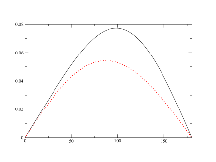
Figure 2: The SSA parameter as function of angle $\phi$. The kinematic region of the calculation is defined by: $\hat{t}$=-0.1 $GeV^{2}$, x=0.3, $\xi$=0.3, S=22. $GeV^{2}$. Solid curve: the result within the unboosted scheme. Dashed curve: the resilt within the boosted scheme.

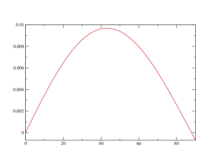
Figure 3: The unboosted scheme SSA parameter from only twist-3 contribution as a function of $\phi$ for the same kinematics as in Fig.2.

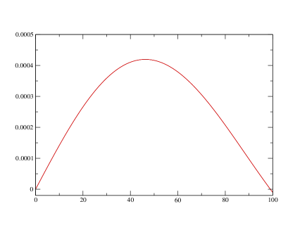
Figure 4: The boosted scheme SSA parameter from only twist-3 contribution as a function of $\phi$ for the same kinematics as in Fig.2.

Figure 5: The boosted scheme generalized parton distribution $H_{1}$ for the $\pi^{\pm}$ case at $t=-0.1\,GeV^{2}$ and $\xi=0.3$.

Figure 6: The boosted scheme generalized parton distribution $H_{3}$ for the $\pi^{\pm}$ case and for the same kinematics as in Fig.5.

Figure 7: The boosted scheme generalized parton distribution $H_{A}$ for the $\pi^{\pm}$ case and for the same kinematics as in Fig.5.

Figure 8: The unboosted scheme generalized parton distribution $H_{1}$ for the $\pi^{\pm}$ case at $t=-0.1\,GeV^{2}$ and $\xi=0.3$.

Figure 9: The unboosted scheme generalized parton distribution $H_{3}$ for the $\pi^{\pm}$ case and for the same kinematics as in Fig.8.

Figure 10: The unboosted scheme generalized parton distribution $H_{A}$ for the $\pi^{\pm}$ case and for the same kinematics as in the Fig.8.

References

• [1] D.MΓΌller et al., Fortschr. Phys. 42 (1994) 101.
• [2] X. Ji, Phys. Rev. D55 (1997) 7114.
• [3] A.V. Radyushkin, Phys.Rev D56 (1997) 5524.
• [4] X. Ji, Phys. Rev. Lett. 78 (1997) 610.
• [5] P.A.M. Guichon, M. Vanderhaegen, Prog. Part. Phys. 41 (1998) 125Β ; X. Ji, J. Phys. G24 (1998) 1181.
• [6] I.V. Anikin, B. Pire, O.V. Teryaev, Phys. Rev. D62 (2000) 071501(R).
• [7] M. Penttinen, M.V. Polyakov, A.G.Shuvaev, M. Strikman, Phys. Lett. B491 (2000) 96; hep-ph/0006321
• [8] A.V. Belitsky, D. MΓΌller, Nucl. Phys. B589 (2000) 611.
• [9] A. Radyushkin, C. Weiss, Phys. Lett. B493 (2000) 332; hep-ph/0010296.
• [10] A.V. Belitsky, D. Muller, A. Kirchner, A. Schafer Twist three analysis of photon electroproduction off pion, hep-ph/0011314
• [11] A.V. Belitsky, A. Kirchner, D. Muller, A. Schafer, Phys. Lett. B510 (2001) 117; hep-ph/0103343
• [12] N. Kivel, M.V. Polyakov, A. SchΓ€fer, O.V. Teryaev, Phys. Lett. B497 (2001) 73; hep-ph/0007315.
• [13] N . Kivel, M.V. Polyakov, M. Vanderhaeghen, Phys. Rev. D63, (2001) 114014.
• [14] K. Goeke, M.V. Polyakov, M. Vanderhaeghen, Hard Exclusive Reactions and the Structure of Hadrons, hep-ph/0106012.
• [15] M.V. Polyakov, C.Weiss, Phys. Rev. D60 (1999) 114017.
• [16] I.V. Anikin, D. Binosi, R. Medrano, S. Noguera and V. Vento work in preparation.
• [17] R.K. Ellis, W. Furmanski, R. Petronzio, Nucl. Phys. B207 (1982) 1.
• [18] A.V. Efremov, O.V. Teryaev, Yad. Phys. 39 (1984) 1517.
• [19] M. Anselmino, A. Efremov, E. Leader, Phys. Rep. 261 (1995) 1.
• [20] O.V. Teryaev, SPIN-96 ProceedingsΒ ; Edited by C.W. de Jager, T.J. Ketel, P.J. Mulders, J.E. Oberski, M. Oskam-Tamboezer. World Scientific, 1997, p.594 .
• [21] HERMES Collaboration, A. Airapetian et al, Measurement of the beam spin azimuthal asymmetry associated with deeply virtual Compton scattering, hep-ex/0106068
• [22] CLAS Collaboration, S. Stepanyan et al, First observation of exclusive deeply virtual Compton scattering in polarized electron beam asymmetry measurements, hep-ex/0107043
• [23] M. Betz and R. Goldflam, Phys. Rev. D28 (1983) 2843.
• [24] X. Ji, W. Melnitchouck and X. Song, Phys. Rev. D56 (1997) 5511.
• [25] M. Traini, V. Vento, A. Mair and A. Zambarda, Nucl. Phys. A614 (1997) 472.
• [26] R. Medrano, S.Noguera and V. Vento, work in preparation.
• [27] R.E. Peirls and J. Yoccoz, Proc. Phys. Soc. London A70 (1957) 381; F. M. Steffens, A. W. Thomas, Prog. Theor. Phys. Suppl. 120 (1995) 145; A. W. Schreiber, A.I. Signal, A.W. Thomas, Phys. Rev. D44 (1991) 2653.
• [28] S. Scopetta and V. Vento, Phys. Lett. B460 (1999) 8; Phys. Lett. B474 (2000) 235; Phys. Lett. B424 (1998) 25.
• [29] I.V. Anikin and V. Vento, work in preparation.
Refer to caption
Refer to caption