DO-TH-01/11

September 2001

revised November 20, 2001

Nonequilibrium evolution in scalar $O(N)$ models with spontaneous symmetry breaking

Jürgen Baacke and Stefan Michalski

Institut für Physik, Universität Dortmund

D - 44221 Dortmund, Germany

We consider the out-of-equilibrium evolution of a classical condensate field and its quantum fluctuations for a scalar $O(N)$ model with spontaneously broken symmetry. In contrast to previous studies we do not consider the large $N$ limit, but the case of finite $N$, including $N=1$, i.e., plain $\lambda\phi^{4}$ theory. The instabilities encountered in the one-loop approximation are prevented, as in the large-$N$ limit, by back reaction of the fluctuations on themselves, or, equivalently, by including a resummation of bubble diagrams. For this resummation and its renormalization we use formulations developed recently based on the effective action formalism of Cornwall, Jackiw and Tomboulis. The formulation of renormalized equations for finite $N$ derived here represents a useful tool for simulations with realistic models. Here we concentrate on the phase structure of such models. We observe the transition between the spontaneously broken and the symmetric phase at low and high energy densities, respectively. This shows that the typical structures expected in thermal equilibrium are encountered in nonequilibrium dynamics even at early times, i.e., before an efficient rescattering can lead to thermalization.

1 Introduction

The investigation of the $O(N)$ vector model at large $N$ has a long-standing history in quantum field theory [1, 2, 3]. The dynamical exploration of nonequilibrium properties of such models has been developed only recently [4, 5, 6, 7, 8, 9]. The nonequilibrium aspects of spontaneous symmetry breaking in particular have been studied in the large-$N$ approximation in Refs. [10, 11, 12, 13, 14].

At finite $N$ there have been several approaches to formulating a Hartree-type interaction between the quantum modes. These lead, in general, to problems with renormalization [15, 16]. On the other hand, without such a back reaction the nonequilibrium systems with spontaneous symmetry breaking run into seemingly unphysical instabilities (see e.g. Fig. 9 in [14] for an illustration). For equilibrium quantum field theory at finite temperature this interaction between quantum modes is taken into account by resummation of bubble diagrams, i.e., by including daisy and super-daisy diagrams. These are essential for studying the phase transitions between the spontaneously broken phase and the phase with restored symmetry. Techniques of bubble resummation have been developed [17, 18, 19] based on the effective action formalism of Cornwall, Jackiw and Tomboulis (CJT) [20]. Recently there have been some new resummation schemes [21, 22, 23, 24] which can be consistently renormalized. While Ref. [21] is restricted to the lowest order two-loop graphs in the action, leading to bubble diagram resummation, the formalism can be extended to include higher order graphs [22, 23, 24]. These approaches can be taken over to a formulation of nonequilibrium equations of motion. Here we restrict ourselves to including two-loop graphs of leading order in $\lambda$ and $1/N$ only; within the CJT formalism this is denoted as Hartree approximation [20].

Having at our disposal a formalism for renormalized finite-$N$ nonequilibrium dynamics we can study the new features introduced by the back reaction between quantum fluctuations in scalar quantum field theories with spontaneous symmetry breaking for finite $N$. A case of particular interest is $N=4$, the $O(4)$ sigma model is widely used as an effective theory for low energy meson interactions. Its nonperturbative aspects may be an essential element for understanding the phenomena observed at RHIC [25]. Such aspects have been discussed previously in [26, 27, 28, 29, 30]. Larger values of $N$ may be realized in grand unified theories, whose nonequilibrium evolution may be of importance in inflationary cosmology [31, 32, 33, 34, 6, 37, 35, 36]; we have included simulations for a suggestive value $N=10$. It should be stressed that the present approximation just constitutes a $1/N$ correction, and the application to low values of $N$ should be taken, therefore, with caution. Indeed, higher order corrections obtained when including the sunset diagram have been found to be of importance [24] in equilibrium quantum field theory. In nonequilibrium quantum field theory the rôle of such higher corrections is being discussed at present [38, 39, 40, 41, 42, 43, 44].

The out-of-equilibrium configuration that has mainly been studied is characterized by an initial state in which one of the components has a spatially homogenous classical expectation value $\phi(t)$. For brevity, and referring to the $O(4)$ case used as a model of low energy pion interactions, we call this component sigma ($\sigma,a=1$), the remaining $N-1$ components pions ($\pi,a=2\dots N$). In the initial state $\sigma$ has a classical value $\phi(0)$, the quantum vacuum is characterized by a Bogoliubov transformation of the Fock space vacuum state, a Bogoliubov transformation characterized by initial masses ${\cal M}_{1}(0)$ and ${\cal M}_{2}(0)$. These masses are determined self-consistently, as are their values at finite times.

The evolution of the system is governed by the classical equation of motion for the field $\phi(t)$ and by the mode equations for the quantum fields $\eta_{a}({\bf x},t)$. The expectation values $\langle\eta_{a}({\bf x},t)\eta_{a}({\bf x},t)\rangle,a=1\dots N$, appear in both equations of motion, this constitutes the quantum back reaction. In the large-$N$ limit one omits the quantum fluctuations of the sigma mode $a=1$ and just considers the Goldstone modes. Here we are able to study the behavior of the $\sigma$ fluctuations as well, we will find that this is a rather important aspect in the critical region.

The plan of this paper is as follows: in section 2 we introduce the model and the potential obtained by bubble diagram resummation in unrenormalized form. Renormalization is discussed in section 3. We present our numerical results in section 4 and discuss their implication for the phase structure of the model. Conclusions are presented in section 5.

2 Formulation of the model

We consider the $O(N)$ vector model with spontaneous symmetry breaking as defined by the Lagrange density

$${\cal L}=\frac{1}{2}\partial_{\mu}\vec{\Phi}\,\partial^{\mu}\vec{\Phi}-\frac{\lambda}{4}\left(\vec{\Phi}^{2}-v^{2}\right)^{2}\;.$$ (2.1)

We consider a quantum system out of equilibrium that is characterized by a spatially homogenous background field. The fields are separated as

$$\Phi_{a}=\phi_{a}(t)+\eta_{a}({\bf x},t)$$ (2.2)

into a classical part $\phi_{a}=\langle\Phi_{a}\rangle$ and a fluctuation part $\eta_{a}$ with $\langle\eta_{a}\rangle=0$. Furthermore, in view of spatial translation invariance it is convenient to decompose the quantum fluctuations via

$$\eta_{i}({\bf x},t)=\int\!\frac{{d^{3}}k}{(2\pi)^{3}2\omega_{0i}}\,\left[a_{\bf k}f_{i}(k,t)e^{i{\bf k}{\bf x}}+a^{\dagger}_{\bf k}f^{*}_{i}(k,t)e^{-i{\bf k}{\bf x}}\right]\;,$$ (2.3)

where $\omega_{0i}=\sqrt{k^{2}+m_{0i}^{2}}$. $m_{0i}$ will be defined below. The subscript $i=1$ denotes the sigma mode ($a=1$), $i=2$ denotes the pion modes ($a=2\dots N$).

In formulating the equations of motion and the renormalization we follow the presentation of Nemoto et al. [21] whose generalization to the nonequilibrium system is straightforward.

We introduce the inverse propagator in the classical background field in an $O(N)$ symmetric form

$${\cal G}_{ab}^{-1}=\left[\Box+{\cal M}_{2}^{2}\right]\delta_{ab}+\frac{\phi_{a}\phi_{b}}{\vec{\phi}^{2}}\left[{\cal M}_{1}^{2}(t)-{\cal M}_{2}^{2}(t)\right]\;.$$ (2.4)

Here ${\cal M}_{1,2}$ are trial masses that will be determined self-consistently. In contrast to equilibrium quantum field theory these masses, as well as the classical field, are allowed to depend on time. This is not the most general parametrization of an inverse propagator; it is sufficiently general if the CJT formalism is restricted to the Hartree-Fock approximation, but not beyond it (see, e.g. [43]). If the inverse propagator has this restricted form, the propagator itself can be written in factorized form in terms of the mode functions $f_{i}(k,t)$. In our application the classical field has just one nonvanishing component $\phi_{1}$; then the inverse propagator has only diagonal elements and these read

$${\cal G}_{ii}(x,x^{\prime})=\int\!\frac{{d^{3}}k}{(2\pi)^{3}2\omega_{0i}}\,\exp\left(i{\bf k}\cdot({\bf x}-{\bf x}^{\prime})\right)f_{i}(k,t_{>})f_{i}^{*}(k,t_{<})$$ (2.5)

(no summation over $i$). If the classical field has more than one nonvanishing component, the Green function can be likewise expressed in terms of mode functions of a coupled system [51, 53]. The occurrence of the mode functions allows for an interpretation in terms of Fock space states which has been used often to define particle numbers that refer explicitly to such a basis. If higher order corrections are included such naive interpretations have to be reconsidered.

Superficially ${\cal M}_{1}$ can be associated with the sigma mass, and ${\cal M}_{2}$ with the pion mass. The actual meaning of these mass type parameters is more subtle, as discussed by Nemoto et al.. We will come back to this point later on.

Using the ansatz (2.4) for the propagator Nemoto et al. derive the CJT effective action, which for a space and time independent configuration is characterized by the effective potential

$$V(\phi,{\cal M}_{1},{\cal M}_{2}) = \frac{1}{2}{\cal M}_{1}^{2}\phi^{2}-\frac{\lambda}{2}\phi^{4}+\frac{1}{2\lambda(N+2)}m^{2}\left\{{\cal M}_{1}^{2}+(N-1){\cal M}_{2}^{2}\right\}$$ (2.6)

$$-\frac{1}{8\lambda(N+2)}\left[(N+1){\cal M}_{1}^{4}+3(N-1){\cal M}_{2}^{4}-2(N-1){\cal M}_{1}^{2}{\cal M}_{2}^{2}+2Nm^{4}\right]$$

$$+\frac{1}{2}\int\frac{d^{4}k}{(2\pi)^{4}}\ln(k^{2}+{\cal M}_{1}^{2})+\frac{N-1}{2}\int\frac{d^{4}k}{(2\pi)^{4}}\ln(k^{2}+{\cal M}_{2}^{2})\;.$$

Here $\phi^{2}=\vec{\phi}^{2}$. We note that our convention for the coupling constant differs from the one in [21], furthermore we have to set $m^{2}=-\lambda v^{2}$.

We can easily generalize this effective potential to obtain the nonequilibrium energy density

$${\cal E} = \frac{1}{2}\dot{\phi}^{2}+\frac{1}{2}{\cal M}_{1}^{2}\phi^{2}-\frac{\lambda}{2}\phi^{4}-\frac{1}{2(N+2)}v^{2}\left\{{\cal M}_{1}^{2}+(N-1){\cal M}_{2}^{2}\right\}$$

$$-\frac{1}{8\lambda(N+2)}\left[(N+1){\cal M}_{1}^{4}+3(N-1){\cal M}_{2}^{4}-2(N-1){\cal M}_{1}^{2}{\cal M}_{2}^{2}+2N\lambda^{2}v^{4}\right]$$

$$+{\cal E}_{{\rm fl},1}+(N-1){\cal E}_{{\rm fl},2}$$

with

$${\cal E}_{{\rm fl},i}=\frac{1}{2}\int\!\frac{{d^{3}}k}{(2\pi)^{3}2\omega_{0i}}\,\left[|\dot{f}_{i}|^{2}+(k^{2}+{\cal M}_{i}^{2}(t))|f_{i}|^{2}\right]\;.$$ (2.8)

The equations of motion can easily be derived by requiring that this energy density be conserved. This is the case if the equation of motion for the field $\phi$ is given by

$$\ddot{\phi}(t)+\left[{\cal M}_{1}^{2}(t)-2\lambda\phi(t)^{2}\right]\phi(t)=0\;,$$ (2.9)

if the quantum modes satisfy the equations of motion

$$\ddot{f}_{i}(k,t)+\left[k^{2}+{\cal M}_{i}^{2}(t)\right]f_{i}(k,t)=0\;,$$ (2.10)

and if the trial masses satisfy, for all $t$, the gap equations

$${\cal M}_{1}^{2}(t) = \lambda\left[3\phi^{2}(t)-v^{2}+3{\cal F}_{1}(t)+(N-1){\cal F}_{2}(t)\right]$$ (2.11)

$${\cal M}_{2}^{2}(t) = \lambda\left[\phi^{2}(t)-v^{2}+{\cal F}_{1}(t)+(N+1){\cal F}_{2}(t)\right]\;.$$ (2.12)

Here ${\cal F}_{i}(t)$ are the fluctuation integrals

$${\cal F}_{i}(t)=\int\!\frac{{d^{3}}k}{(2\pi)^{3}2\omega_{0i}}\,|f_{i}(k,t)|^{2}\;.$$ (2.13)

The gap equations incorporate the resummation of bubble diagrams.

For a time-dependent problem we have to specify initial conditions. We choose at $t=0$ a value of the classical field $\phi_{0}=\phi(0)$ different from its value in the equilibrium ground state, which is given by $v$ apart from quantum corrections. The initial mass parameters $m_{i0}={\cal M}_{i}(0)$ are obtained by solving the gap equations (2.11) and (2.12) at $t=0$, i.e., by finding the extremum of the effective potential at a fixed value of $\phi=\phi_{0}$. So the initial configuration is an equilibrium configuration with an externally fixed field $\phi_{0}$. When the field is allowed, for $t>0$, to become an internal dynamical field the nonequilibrium evolution sets in.

The equations of motion and the gap equations still contain divergent integrals and need to be replaced by renormalized ones. These will be derived in the next section.

Before continuing in developing the formalism we would like to come back to the discussion of the masses. The mass parameters ${\cal M}_{i}$ naively represent the effective masses for the $\sigma$ and $\pi$ fluctuations. In finite temperature quantum field theory one expects massless quanta, the Goldstone modes, if the field is in the temperature-dependent minimum of the effective potential in the broken symmetry phase. Likewise, in the nonequilibrium evolution of large-N systems it has been found [10, 11, 12, 13, 14] that the mass of the fluctuations goes to zero in the broken symmetry phase as the classical field approaches an equilibrium value. In some sense that is trivial there, because the mass of the fluctuations appears in the classical equation of motion as well, and in equilibrium we must have $\ddot{\phi}=-{\cal M}^{2}(t)\phi=0$. Here the situation is more complicated and indeed we will find that ${\cal M}_{2}^{2}(t)$ will not go to zero at late times, even if the classical field settles at some constant value. Likewise, in the static case, at finite temperature, one finds that the “pion” mass ${\cal M}_{2}$ is not in general zero, the question has been rised, whether Goldstone’ s theorem is violated by the approximation or otherwise.

The interpretation of the masses and the value of the pion mass in the present context have been discussed extensively in Refs.[21, 23]. These authors argue that ${\cal M}_{2}$ is not to be interpreted as the pion mass, but as a variational parameter which does not necessarily have an immediate physical interpretation. The ansatz for the inverse Green function and in consequence the effective potential have full $O(N)$ symmetry. The field $\phi$ appearing there is the absolute value of the field $\phi_{a}$. Therefore by symmetry the pion mass must trivially be zero in the minimum of the effective potential, which is an $O(N-1)$ sphere. Nemoto et al. show that trivially the appropriate second derivatives of the effective potential lead to a vanishing pion mass. Likewise ${\cal M}_{1}$ is another parameter characterizing the Green function and is different from the sigma mass which is given by

$$m_{\sigma}^{2}=2v^{2}(\frac{d{\cal M}_{1}^{2}}{d\phi^{2}}-2\lambda)\;.$$ (2.14)

This is equal to $2\lambda v^{2}$ on the tree level only.

It is instructive to do the simple algebra of taking second derivatives of an $O(N)$ symmetric function:

$$\frac{\partial^{2}f(\vec{\phi}^{2})}{\partial\phi_{a}\partial\phi_{b}}=2\delta_{ab}f^{\prime}(\vec{\phi}^{2})+4\phi_{a}\phi_{b}f^{\prime\prime}(\vec{\phi}^{2})\;.$$ (2.15)

The pion mass is the second derivative perpendicular to the direction of $\phi_{a}$, so it is given by the first term and vanishes if $f^{\prime}(\vec{\phi}^{2})=0$, which defines the minimum. This corresponds precisely to the first derivative of the potential appearing in the classical equation of motion. We note that this effective mass is given by

$${\cal M}_{\rm cl}^{2}=\biggl{(}{\cal M}_{1}^{2}(t)-2\lambda\phi^{2}(t)\biggr{)}\;.$$ (2.16)

It vanishes trivially if the field settles at late times at some constant value.

The masses $m_{\sigma}^{2}$ and ${\cal M}_{\rm cl}^{2}$ determine the fluctuations of the classical field $\phi$ near the minimum of the effective potential in analogy to the tree level masses of the sigma and pion fields. If all higher corrections were included, one would expect these masses to determine the exact propagator near $k^{2}=0$. In this sense the vanishing of ${\cal M}_{\rm cl}^{2}$ entails a pole of the pion propagator at $k^{2}=0$. However, contrary to the large-$N$ limit, ${\cal M}_{\rm cl}^{2}$ is not the mass that determines the fluctuations $f_{2}$ and, thereby, the “pion” propagator ${\cal G}_{22}$.

3 Renormalization

The renormalization of the effective potential has been discussed in [21] and [22]. As stated in the latter publication both formulations are equivalent, here we follow the one of Nemoto et al., employing the auxiliary field method, in which the counterterms in the effective potential are introduced via the the trial masses:

$$\delta{\cal E}=Av^{2}{\cal M}_{1}^{2}+Bv^{2}{\cal M}_{2}^{2}+\frac{1}{2}C{\cal M}_{1}^{4}+\frac{1}{2}(N-1)D{\cal M}_{2}^{4}\;.$$ (3.1)

Divergent and finite parts of the fluctuation integrals ${\cal F}_{i}$ and of the fluctuation energy densities have been analyzed in [9, 45] using a perturbation expansion in the “potentials”

$${\cal V}_{i}(t)={\cal M}_{i}^{2}(t)-{\cal M}_{i}^{2}(0)\;.$$ (3.2)

As the definition of the Green functions (2.5), the expressions for the energy densities (2.8) and for the fluctuation integrals (2.13), as well as the equations (2.10) satisfied by the mode functions are entirely analogous to those in [45], the expansions derived there can be applied here in the same way. In the power series expansion of the energy densities with respect to ${\cal V}_{i}$ the zeroth, first and second order terms are UV divergent, while in the fluctuation integrals it is the zeroth and first order terms. In dimensional regularization the powers of ${\cal V}_{i}$ can be arranged with powers of $m_{i0}^{2}$ into powers of ${\cal M}_{i}^{2}$. The expansion then reads

$${\cal E}_{{\rm fl},i} = \frac{1}{64\pi^{2}}\left[{\cal M}_{i}^{4}(-L+\ln\frac{m_{i0}^{2}}{\mu^{2}})-2{\cal M}_{i}^{2}m_{0i}^{2}+\frac{1}{2}m_{i0}^{4}\right]+{\cal E}_{{\rm fl},i}^{\rm fin}$$ (3.3)

$${\cal F}_{i} = \frac{1}{16\pi^{2}}\left[{\cal M}_{i}^{2}\left(-L+\ln\frac{m_{i0}^{2}}{\mu^{2}}\right)-m_{0i}^{2}\right]+{\cal F}_{i}^{\rm fin}\;.$$ (3.4)

Here

$$L=\frac{2}{\epsilon}-\gamma+\ln 4\pi\;,$$ (3.5)

$\mu$ is the renormalization scale, and $m_{i0}$ are the mass parameters appearing in the fluctuation integrals. In order to avoid bad initial singularities [46, 47, 48] they have to be chosen as $m_{i0}={\cal M}_{i}(0)$, the “initial masses”. Finally the finite fluctuation integrals are defined by subtracting the UV divergent parts under the momentum integral via

$${\cal E}_{{\rm fl},i}^{\rm fin} = \frac{1}{2}\int\!\frac{{d^{3}}k}{(2\pi)^{3}2\omega_{0i}}\,\left[|\dot{f}_{i}|^{2}+(k^{2}+{\cal M}_{i}^{2})|f_{i}|^{2}\right.$$

$$\hskip 28.45274pt\left.-2\omega_{i0}^{2}-{\cal V}_{i}+\frac{{\cal V}_{i}^{2}}{4\omega_{i0}^{2}}\right]$$

$${\cal F}_{i}^{\rm fin} = \frac{1}{2}\int\!\frac{{d^{3}}k}{(2\pi)^{3}2\omega_{0i}}\,\left[|f_{i}|^{2}-1+\frac{{\cal V}_{i}}{2\omega_{i0}^{2}}\right]\;.$$ (3.7)

The subtractions used here are analytically equivalent to a numerically more sophisticated procedure used in [9]. The subtracted integrals are UV finite.

From Eqs. (3.3) and (3.4) it is evident that the divergent parts $\propto L$ are independent of the initial masses $m_{i0}^{2}$ and thereby of the initial conditions. Exactly as in equilibrium theory [21] the divergent parts can be removed by choosing the counter terms (3.1) as $A=B=0$ and as

$$C=D=\frac{1}{64\pi^{2}}L\;.$$ (3.8)

With this choice the energy density as well as the gap equations become finite. The equations of motion are not affected. The energy density is obtained simply by replacing the fluctuation energies by the right hand sides of (3.3) omitting the term proportional to $L$. Likewise the renormalized gap equations are obtained by replacing the fluctuation integrals by the right hand sides of (3.4) without the term proportional to $L$. In our numerical computations the renormalization scale $\mu$ has been taken equal to the sigma mass. As long as the ratio of $\mu$ and the relevant masses is far from the Landau pole, i.e., $m^{2}/\mu^{2}\ll\exp 16\pi^{2}/\lambda$ the dependence on the renormalization scale is weak. This is the condition under which the $\Phi^{4}$ theory can be treated as a low energy effective theory. For our numerical simulations with $\lambda=1$ this condition is fulfilled.

The gap equations for the masses have to be solved once, at $t=0$. By subtracting these equations at $t=0$ from the general gap equations one obtains the renormalized gap equations for the potentials ${\cal V}_{i}$. These read explicitly

$${\cal V}_{1} = \lambda\left[3(\phi^{2}-\phi_{0}^{2})+3{\cal F}_{1}^{\rm fin}+(N-1){\cal F}_{2}^{\rm fin}\right.$$

$$\left.+\frac{3}{16\pi^{2}}\ln\frac{m_{10}^{2}}{\mu^{2}}{\cal V}_{1}(t)+\frac{N-1}{16\pi^{2}}\ln\frac{m_{20}^{2}}{\mu^{2}}{\cal V}_{2}(t)\right]$$

$${\cal V}_{2} = \lambda\left[(\phi^{2}-\phi_{0}^{2})+{\cal F}_{1}^{\rm fin}+(N+1){\cal F}_{2}^{\rm fin}\right.$$

$$\left.+\frac{1}{16\pi^{2}}\ln\frac{m_{10}^{2}}{\mu^{2}}{\cal V}_{1}(t)+\frac{N+1}{16\pi^{2}}\ln\frac{m_{20}^{2}}{\mu^{2}}{\cal V}_{2}(t)\right]\;.$$

These linear equations can be solved easily for ${\cal V}_{i}(t),i=1,2$ using a time-independent matrix. This matrix is analogous to the factor ${\cal C}=(1+(\lambda/16\pi^{2})\ln(m^{2}/m_{0}^{2}))^{-1}$ appearing in the large-$N$ case [45].

The numerical implementation has been described in several previous publications (see e.g. [9]), so we do not repeat this here. The accuracy of the computations is monitored by veryfying the energy conservation, which holds with a typical precision of five significant digits.

We finally mention the problem of initial singularities that appears in the context of renormalization [46, 47, 48]. These can be avoided by modifying the initial quantum ensemble via a suitable Bogoliubov transformation. This can be done in the present model as well. For the values of the couplings and initial parameters considered here the initial singularities are numerically unimportant and have been disregarded, therefore.

4 Results and discussion

4.1 Numerical simulations

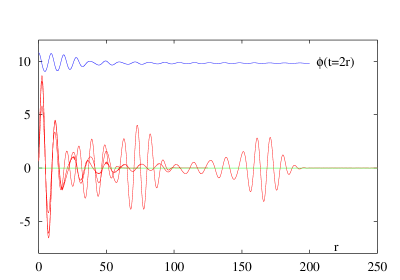
We have performed numerical simulations for the cases $N=1$, $N=4$ and $N=10$. The coupling constant was taken to be $\lambda=1$ and we have varied the initial value for the field $\phi_{0}=\phi(0)$. We have considered only values $\phi_{0}>v$, as for smaller values the initial mass $m_{20}={\cal M}_{2}(0)$ becomes imaginary. The region $\phi<v$ is only explored dynamically. We display the time evolution of the classical amplitude $\phi(t)$ for the parameters $N=4,\lambda=1$ in Figs. 1a-c, for initial amplitudes $\phi_{0}=1.3v<\sqrt{2}v$, $\phi_{0}=1.445v\simeq\sqrt{2}v$ and $\phi_{0}=1.6v>\sqrt{2}v$.

Figure 1a: Time evolution of the classical field $\phi$ for $\phi_{0}<\sqrt{2}v$ (broken symmetry phase). Field amplitude and time are in units of $v$ and $v^{-1}$, respectively. Parameters are $N=4$, $\lambda=1$, and $\phi_{0}=1.3v$.

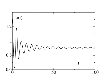
For the tree level potential the value $\phi=\sqrt{2}v$ is the value for which the energy is equal to the height of the barrier ($N=1$) or the top of the Mexican hat ($N>1$). We will discuss the physics associate with the three ranges of parameters below.

Figure 1b: Time evolution of the classical field $\phi$ for $\phi_{0}\simeq\sqrt{2}v$ (critical region). Parameters as above but $\phi_{0}=1.445v$.

Figure 1c: Time evolution of the classical field $\phi$ for $\phi_{0}>\sqrt{2}v$ (symmetric phase). Parameters as above but $\phi_{0}=1.6v$.

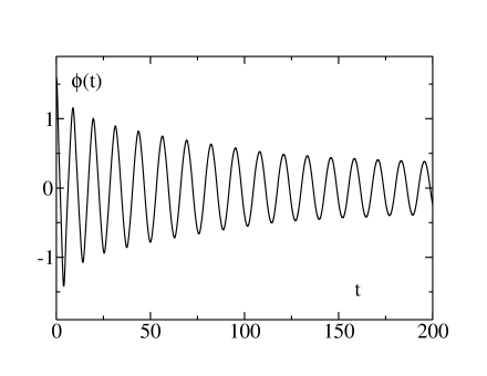
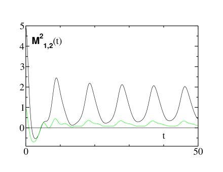
In the nonequilibrium evolution of models with spontaneous symmetry breaking both squared masses ${\cal M}_{1,2}^{2}$ can in general take negative values. In large-$N$ dynamics it is well known [12, 13, 14] that in this situation the fluctations increase exponentially and drive the squared masses back to positive values. This stabilizes the system dynamically and prevents an unphysical behavior in which an exponentially increasing amount of quantum energy, taken from the vacuum, is converted into classical one. Our first essential observation is that for all parameter sets and initial values this stabilization takes place for finite $N$ as well. We display a typical time evolution of the classical field and of the squared masses ${\cal M}_{1,2}^{2}$ in Fig. 2a and Fig. 2b, based on the parameters $N=4,\lambda=1$, and $\phi_{0}=1.4v$. In Fig. 2a both squared masses are seen to become negative at early times and to reach positive values at late times. In Fig. 2b one sees the evolution of the energy of the fluctuations which is very strong in the time range where the squared masses are negative.

Figure 2a: Time evolution of the masses ${\cal M}_{1,2}^{2}$. Parameters are $N=4$, $\lambda=1$, and $\phi_{0}=1.4v$. The upper curve is ${\cal M}_{1}^{2}$.

Figure 2b: Time evolution of the energy densities. Parameters as in Fig. 2a. Displayed are the classical energy density, the fluctuation energy density including finite renormalization terms and the total energy density.

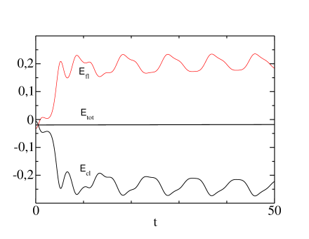
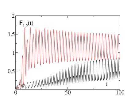
The classical minimum of the energy is at $E_{0}=-\lambda v^{4}/4$, i.e., $E_{0}=-.25$ for this parameter set. So essentially all the energy is transferred to fluctuations within a few oscillations of the condensate field $\phi$. In Fig. 2c we display the two fluctuation integrals as functions of time for $\phi_{0}=2v$, again for $N=4$ and $\lambda=1$, i.e. in the symmetric phase. The pion fluctuations are seen to develop rather quickly, while the sigma fluctuations only develop at later times.

Figure 2c: Time evolution of the fluctuations integrals. Parameters as in Fig. 2a, however with $\phi_{0}=2v$. upper curve: pion fluctuations, lower curve: sigma fluctuations.

The main aspect we will consider here is the phase structure of the model. In thermal quantum field theory one expects a phase with spontaneously broken symmetry at low temperature, and symmetry restoration at high temperature. Here we have a microcanonical description, so instead of temperature we specify the energy which in turn is determined by the initial value $\phi_{0}$. As already mentioned the system will not thermalize in the approximation used here, but it is characterized at late times by limiting values, or time averages, attained by the various masses, and by the classical field $\phi$. The latter can be compared with the temperature-dependent vacuum expectation value $v(T)$, the former ones are associated to correlation lengths.

Figure 3a: The late-time amplitude as a function of the initial amplitude. Parameters are $N=1$ and $\lambda=1$.

Figure 3b: Same as Fig. 3a, for $N=4$ and $\lambda=1$.

Figure 3c: Same as Fig. 3a, for $N=10$ and $\lambda=1$

Classically the spontaneously broken phase is expected to be situated in the interval $v<\phi_{0}<\sqrt{2}v$. For larger values of $\phi_{0}$ one should be in the phase of restored symmetry. Since the effective potential receives quantum corrections the boundaries of these intervals will be slightly shifted, for brevity we continue to use the classical values in the following discussion.

4.2 Late time behavior of the classical field

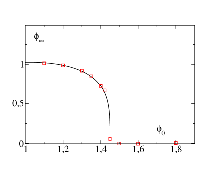
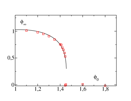
We first consider $\phi_{\infty}(\phi_{0})$, the value of $\phi$ averaged at late times, which can be considered as an order parameter, replacing the vacuum expectation value $v(T)$ of finite temperature field theory. In the analysis of the broken symmetry phase in the large-$N$ limit it was observed [12, 13, 14] that the value of $\phi$ at late times has a specific and universal dependence on the initial value $\phi_{0}$, given at zero temperature by

$$\phi_{\infty}\simeq\left[\phi_{0}^{2}\left(2v^{2}-\phi_{0}^{2}\right)\right]^{1/4}$$ (4.1)

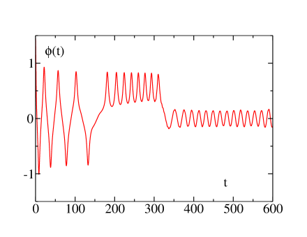
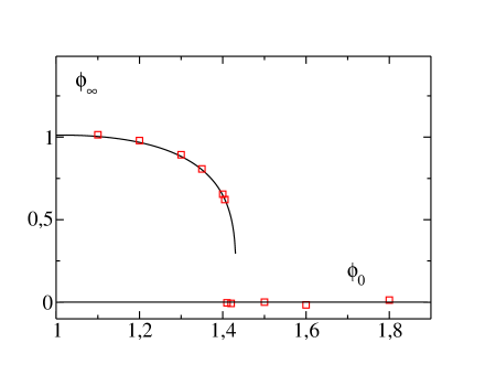
We find that this is the case for finite $N$ as well. The dependence $\phi_{\infty}(\phi_{0})$ is shown in Figs. 3a-c for $N=1,4$ and $10$, respectively, the curves are rough fits of the form of Eq. 4.1, taking into account a slight shift of the point of “phase transition” $\phi\simeq\sqrt{2}v$. Such a functional behavior is typical of a phase transition of second order. In a first oder phase transition the vacuum expectation value of the true minimum jumps at the phase transition from the broken symmetry minimum to the symmetric one. As the functional behavior of Eq. (4.1) has an infinite slope at the critical point it is hard to decide from numerical data whether $\phi_{\infty}$ near $\phi_{0}=\sqrt{2}v$ goes to zero continously or via a discontinuity. The results strongly indicate that the transition is discontinuous. This is suggested as well by the time evolution of $\phi$ displayed in Fig. 1b. There seems to be a minimum at $\phi=0$ and another one near $\phi\simeq.5v$, as one knows it from typical finite temperature potentials of first order phase transitions. However, even if the transition is first order, it is very close to a second order one. In thermal equilibrium a first order phase transition is expected [21, 24], it becomes second order only after including higher loop corrections. Fig. 1b puts in evidence that the time averaging is problematic near the phase transition; this implies that the functional dependence the “order parameter” $\phi_{\infty}$ near $\phi_{0}\simeq\sqrt{2}v$ is not determined with high precision.

We would like to remark that we have chosen special initial conditions which allow the classical field to move in one fixed direction only. So the system cannot see the difference between a double-well and a Mexican hat potential. Imposing more general initial conditions [53] may lead to an improved understanding of the nonequilibrium properties of the system. Such a generalization may be useful especially near the transition point $phi_{0}\simeq\sqrt{2}v$.

For $\phi>\sqrt{2}v$ the time average of $\phi$ vanishes as $t\to\infty$, and in fact already at an early stage of evolution. However, the amplitude of the oscillations decreases very slowly, if at all. So, although the order parameter $\phi_{\infty}$ shows the behavior expected in the symmetric phase of a thermal system, and although the system becomes essentially stationary, it shows no resemblance to a system in thermal equilibrium with a constant value of $\phi$. We will further analyze this phase, below.

4.3 Late time behavior of the masses

Another set of variables characteristic for the phase structure of the $O(N)$ model in equilibrium are the mass scales or correlation lengths. In the broken symmetry phase we expect a vanishing pion mass and a nonzero value of the field $\phi$. In section 2 we have discussed to some extent the problem of the Goldstone mass, which should not be identified naively with ${\cal M}_{2}$; rather, we have proposed to associate it with the “classical mass” ${\cal M}_{\rm cl}$ defined in Eq. (2.16). Both masses would coincide in the large-$N$ limit.

Figure 4: The various masses averaged at late times (t=300), as functions of the initial amplitude. Squares: ${\cal M}_{1}^{2}$, diamonds: ${\cal M}_{2}^{2}$, circles: ${\cal M}_{\rm cl}^{2}$. Parameters are $N=4$ and $\lambda=1$.

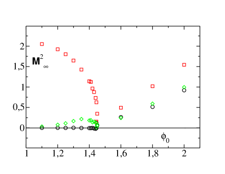
Likewise, the sigma mass is not given naively by ${\cal M}_{1}$. We plot the three squared masses ${\cal M}_{1}^{2}$, ${\cal M}_{2}^{2}$, and ${\cal M}_{\rm cl}^{2}$ as functions of $\phi_{0}$ in Fig. 4, for $N=4,\lambda=1$. ${\cal M}_{\rm cl}^{2}$ is seen to be almost zero for $v<\phi_{0}<\sqrt{2}v$ and to increase for larger values of $\phi_{0}$, as expected for the Goldstone mass. The mass ${\cal M}_{2}^{2}$ is small for $v<\phi_{0}<\sqrt{2}v$ but definitely different from zero, and increases likewise for $v>\sqrt{2}v$. The “sigma mass” ${\cal M}_{1}$ is different from zero everywhere, except near $\phi_{0}=\sqrt{2}v$.

The formalism presented here contains of course the limit $N\to\infty$. This limit is obtained by letting $\lambda\propto 1/N$ and $\phi,\phi_{0},v\propto\sqrt{N}$. In this limit the quantum fluctuations $\eta_{1}$ become irrelevant, and so does ${\cal M}_{1}$. The “pion” mass ${\cal M}_{2}$ and the “classical mass” ${\cal M}_{\rm cl}$ become identical to the mass ${\cal M}$ of Refs. [11, 12, 13, 14] or $\chi(t)$ of Ref. [10]. In the broken symmetry phase the instability pushes this mass to zero. Here, for finite $N$, we find ${\cal M}_{2}^{2}$ to remain positive though small in the broken symmetry phase, while ${\cal M}_{\rm cl}^{2}$ again vanishes. It should be mentioned that the vanishing of the classical mass ${\cal M}_{\rm cl}^{2}$ in the broken symmetry phase is due to the fact that the field $\phi(t)$ settles at a constant nonzero value. For the fluctuation mass ${\cal M}_{2}^{2}$ the dynamics of backreaction only forces it to be nonnegative. In the large-$N$ limit the identity of the two masses ${\cal M}^{2}={\cal M}_{2}^{2}={\cal M}_{\rm cl}^{2}$ entails their vanishing at late times, as expected from the Nambu-Goldstone theorem. The situation found here at large times is analogous to the one found in thermal equilibrium [21, 23] (see section 2).

For a phase transition of second order the $\sigma$ mass, all mass scales are expected to vanish at the “critical point”, i.e., for $\phi_{0}\simeq\sqrt{2}v$. We see from Fig. 4 that this is almost the case. For a first order phase transition the curvature of the potential in the broken symmetry minimum decreases when approaching the phase transition, but remains positive up to and beyond the phase transition. Above the phase transition the curvature in the symmetric minimum increases again. The fact that ${\cal M}_{1}^{2}$ does not really reach zero may of course be a deficiency of our numerics. We point out, however, that critical behavior implies large length and also time scales, so that in this neighborhood the time averaging is precarious and the late time values are not very precise. It is not clear whether the field in Fig. 1b will jump back and forth between the various minima at later times again and, if it does, whether this is not a consequence of accumulated tiny numerical errors. We again conclude that, if the phase transition is of first order, it is “weakly first order”. While we have mostly presented results for $N=4$, we find similar results for $N=1$ and $N=10$. For $N=1$ the mass ${\cal M}_{2}$ is of course meaningless.

As we have mentioned above, in the symmetric phase the time average of the field $\phi$ becomes zero at late times, while the field itself continues to oscillate with essentially constant amplitude, implying that the time average $\langle\phi^{2}\rangle$ of the squared field remains different from zero. This implies that the masses ${\cal M}_{1}^{2}$ and ${\cal M}_{2}^{2}$ necessarily have different time averages; indeed the classical field contributes with $3\lambda\langle\phi^{2}\rangle$ to $\langle{\cal M}_{1}^{2}\rangle$ but only with $\lambda\langle\phi^{2}\rangle$ to $\langle{\cal M}_{2}^{2}\rangle$. Actually even the quantum fluctuations ${\cal F}_{1}$ and ${\cal F}_{2}$ have different time averages. This is contrary to what one expects in a symmetric equilibrium phase. The problem is inherent in the initial conditions which necessarily require a high excitation and the choice of direction in $O(N)$ space. It is appropriate at this point to compare with a $\Phi^{4}$ model without spontaneous symmetry breaking, i.e., with $m^{2}=-\lambda v^{2}>0$. There again the classical field oscillates around $\phi=0$ with slowly decreasing amplitude.

Figure 5: The various masses averaged at late times (t=300), as functions of the initial amplitude for a model without symmetry breaking, $N=4$, $\lambda=1$, $v^{2}=-m^{2}/\lambda=-1$. Symbols as in Fig. 4.

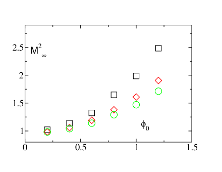
Again the time average of mass ${\cal M}_{1}^{2}$ remains different from the one of ${\cal M}_{2}^{2}$ pertaining to the fields $\eta_{a}$ with $a=2\dots N$. We show in Fig. 5 the dependence of the late time averaged masses for this manifestly symmetric theory. The close resemblance with the behavior in the high energy phase of the model with spontaneous symmetry breaking is obvious. The difference between the masses is not related to spontaneous symmetry breaking but to the fact that the system is prepared in a non-symmetric state.

While the behavior of masses ${\cal M}_{2}^{2}$ and ${\cal M}_{\rm cl}^{2}$ found here essentially reproduces the one of ${\cal M}^{2}$ in the large-$N$ limit we have seen here, that the sigma mass contains valuable information about the nature of the phase transition, not available in the large-$N$ limit, and that the sigma fluctuations are relevant for finite $N$.

4.4 Correlations

Correlations of mode functions have been discussed in various publications [10, 28, 13, 29]. If one thinks of the $N=4$ model as a model for pion production, possibly displaying structures like disordered chiral condensates, it is the correlations between the pion fluctuations ($i=2$ or $a=2\dots N$) which are relevant. In the large-$N$ limit these are the only available correlations. It was found in a large-$N$ computation including the full backreaction [13] that the correlation length grows with time in the broken symmetry phase. Kaiser [28], analyzing the correlations in the initial phase, before back reaction sets in, suggested the occurrence of large correlation lengths. Hiro-Oka and Minakata [29] performing a computation with backreaction, however unrenormalized and with a different Hartree factorization, suggested that the correlation length remains small.

The pion correlations are obtained [13] as the Fourier-Bessel transform

$$C(r,t) = \langle\eta_{2}({\bf x},t)\eta_{2}({\bf 0},t)\rangle=\int\!\frac{{d^{3}}k}{(2\pi)^{3}2\omega_{02}}e^{i{\bf k}\cdot{\bf x}}|f_{2}(k,t)|^{2}$$ (4.2)

$$= \frac{1}{2\pi^{2}r}\int_{0}^{\infty}dk~{}k\sin(kr)|f_{2}(k,t)|^{2}\;.$$

We have performed a series of simulations illustrating the transition from $N\to\infty$ to finite $N$. Fig. 6a shows the correlation functions $rC(r)$ at times $t=30$, $50$ and $100$ for $\lambda\cdot N=1$, with $N=\infty$, $10$ and $4$.

Figure 6a: Equal-time correlations of pion fluctuations. We plot $rC(r)$, with $C(r)$ as defined in Eq. (4.2), at times $t=30$, $50$, $100$, for parameters $v=\sqrt{N}$, $\lambda=1/N$, $N=4$, $10$ and for $N\to\infty$. Initial amplitude $\phi_{0}=1.024v$. On top the amplitude $\phi(t)/v$ for $N\to\infty$.

Figure 6b: Equal-time correlations of pion fluctuations; parameters $N=4$, $\lambda=1/4$, $v=2$, initial amplitude $\phi_{0}=1.2v$.

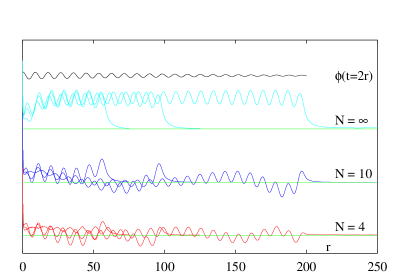
The initial amplitude is $\phi_{0}\simeq 1.024v$ implying in all cases $m_{20}\simeq 0.2$. It is seen that there are long range correlations in all cases. They are seemingly related to or actually generated by the oscillations of the classical field. Its amplitude is displayed in the same figure for the case $N\to\infty$, the finite $N$ amplitudes behave very similarly. The correlations are positive throughout for the large-$N$ case. For $N=10$ and $N=4$ they alternate in sign in the central region at late times. So at small $N$, in particular at $N=4$, these results certainly do not suggest a growth of positively correlated domains but rather a wash-out implied by the alternating signs. In fact the size of a positively correlated region is essentially of the order of an oscillation period of the sigma field.

The close relationship between the oscillations of the classical field and the correlations is further demonstrated in Fig. 6b. For $N=4,\lambda=1$ and an initial value $\phi_{0}=1.2v$ the oscillations of the classical field decay rather quickly, and so do the correlations. This means that one has to be cautious with their interpretation: these correlations are not due to an interaction between field fluctuations but are generated by the coherence of such fluctuations with an external source. This is not necessarily the wrong physics, but certainly this feature is inherent in the mean field approach.

4.5 Momentum spectra

In the large-$N$ limit one of the most pronounced characteristic of the momentum spectra of the “pion” fluctuations is the occurrence of parametric resonance bands. These develop already in the early stage of evolution, before backreaction sets in. Then the time dependence of the classical field is described by Jacobian elliptic functions, and the fluctuations are solutions of the Lamé equation. These solutions have been derived and discussed extensively in [11, 12, 13].

For our finite-$N$ system the early time behavior of the classical field and of the pion modes is the same as in the large-$N$ limit, as before the onset of fluctuations both ${\cal M}_{\rm cl}^{2}$ and ${\cal M}_{2}^{2}$ are approximatley equal to $\lambda(\phi^{2}-v^{2})$, while ${\cal M}_{1}^{2}\simeq\lambda(3\phi^{2}-v^{2})$. The analysis of the pion fluctuations can be taken over from Ref. [11], therefore. For $\phi_{0}<\sqrt{2}v$ the parametric resonance band is given by

$$\lambda\left(v^{2}-\frac{\phi_{0}^{2}}{2}\right)<k^{2}<\frac{\lambda}{2}\phi_{0}^{2}\;,$$ (4.3)

as given in Ref. [11]. For $\phi_{0}>\sqrt{2}v$ parametric resonance occurs (see Appendix A) in the momentum interval

$$0<k^{2}<\frac{\lambda}{2}\phi_{0}^{2}\;.$$ (4.4)

In Figs. 7 and 8 we plot the integrands of the various fluctuation integrals ${\cal F}_{i}$, i.e.

$$\frac{k^{2}}{2\pi^{2}2\omega_{i0}}\left(|f_{i}(k,t)|^{2}-1+\frac{{\cal V}_{i}}{2\omega^{2}_{i0}}\right)$$ (4.5)

as functions of $k$.

Figure 7a: Spectrum of sigma fluctuations in the broken symmetry phase. We display the integrand defined in Eq. (4.5) of the fluctuation integral as a function of $k$ for $\lambda=1$, $v=1$, $\phi_{0}=1.2v$ at $t=100$.

Figure 7b: Spectrum of pion fluctuations in the broken symmetry phase. Notation and parameters as in Fig. 7a.

Figure 8a: Spectrum of sigma fluctuations in the symmetric phase. Notation and parameters as in Fig. 7a, however $\phi_{0}=2v$.

Figure 8b: Spectrum of pion fluctuations in the symmetric phase. Notation and parameters as in Fig. 7a, however $\phi_{0}=2v$.

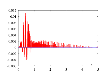
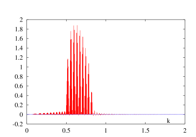
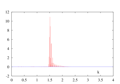
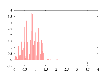
As seen in Figs. 7b and 8b parametric resonance indeed dominates the pion fluctuations within the momentum intervals (4.3) and (4.4) in the broken symmetry and in the symmetric phase respectively. The sigma fluctuations are unimportant in the broken symmetry phase, as displayed in Fig. 7a. In the symmetric phase they develop a pronounced resonance which seemingly becomes sharper and sharper as time increases. The position of the resonance can be obtained by considering the periodicity $T$ of the square of the classical field and the frequency of the “sigma” fluctuations; one expects $k^{2}+\langle{\cal M}_{1}^{2}\rangle\simeq 4\pi^{2}/T^{2}$. The empirical (“measured”) values of $T$ and $\langle{\cal M}_{1}^{2}\rangle$ for the simulation with our parameter set yield $k\simeq 1.5$ in agreement with Fig. 8a. As the resonance is due to a time-dependent mass term, it should be situated in a resonance band, as indeed suggested by Fig 8a. For this resonance band the early time analysis does not apply, as the sigma fluctuations evolve at a time when backreaction due to pion fluctuations has already modified the equation for the condensate field $\phi(t)$, see Fig. 2c. It should be noted that an analoguos resonance appears in the spectrum of sigma (longitudinal) fluctuations in the $\Phi^{4}$ model without spontaneous symmetry breaking, while the pion (transverse) fluctuations display a broad parametric resonance band. So again the difference between the fluctuations parallel and orthogonal to the classical field is not related to spontaneous breaking but to the non-symmetry of the state.

4.6 A naive dynamical effective potential

As we have seen, the behavior of the system below $\phi_{0}=\sqrt{2}v$ displays the features of a spontaneously broken phase in a rather convincing way, while for the symmetric phase the non-symmetric initial conditions remain manifest even at late times. The amplitude of oscillations of the classical field does not go to zero even if we extend the simulation to times beyond which we believe our numerical reliability.

Figure 9a: Evolution of the potential energy. Definition as in subsection 4.6. Parameters: $v=1$, $\lambda=1$, and $\phi_{0}=1.2v$.

Figure 9b: Evolution of the potential energy. Parameters as in Fig. 9a, however $\phi_{0}=2v$.

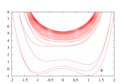
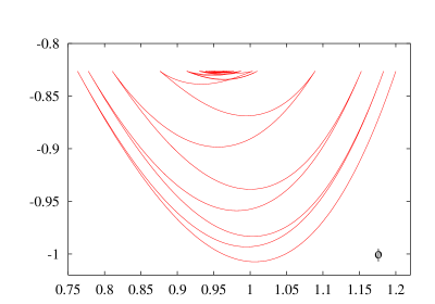
The evidence for symmetry restoration remains indirect, therefore. So it might be useful to have yet another criterion. This is given by the dynamics of the classical field. In a rather trivial way the potential that yields the “force” experienced by the classical field is given by the potential energy, obtained by subtracting the kinetic energy from the total energy, $V_{\rm pot}=E-\dot{\phi}^{2}/2$. This potential is of course time-dependent and is explored only within the range of oscillations of the field. We display this potential energy in Figs. 9a and 9b for the broken and for the symmetric phase, respectively. It is seen that the positions of minima shift from $\phi=\pm v$ to smaller absolute values in the broken symmetry phase, while in the symmetric phase the separate minima entirely disappear after a few oscillations and a new minimum appears at $\phi=0$.

5 Conclusions

We have presented here an analysis of nonequilibrium dynamics in $O(N)$ models with spontaneous symmetry breaking at finite $N$ in a bubble-resummed one-loop approximation. This has allowed us to study some new features of such systems, not accessible to the large-$N$ or one-loop approximations.

We have found that the back-reaction of the quantum fluctuations on themselves prevents, as in the large-$N$ approximation, a catastrophic instability of the system as found in the one-loop approximation. The mechanism is, like in large-$N$, an exponential evolution of those quantum fluctuations whose effective mass squared has become negative, pushing this mass squared back to positive values.

The dependence on the initial conditions displays features of an expected phase transition between a regime with spontaneous symmetry breaking and a symmetric phase. A more detailed analysis of nonequilibrium dynamics in the critical region may provide new insights into the nature of the phase transition.

Our approach provides an new tool for performing studies of nonequilibrium evolution in scenarios typical of heavy ion collisions [25] or of the dynamics of inflation in the early universe [31], using appropriate models like the $O(4)$ sigma model or realistic grand unified theories. It should be especially useful for studying phase transitions and critical behavior in an nonequilibrium context. It would be useful to extend this study to more general initial conditions exploiting more of the multi-dimensional mexican hat structure of the potentials in models with $N\neq 1$. The techniques using coupled-channel Green functions are available [49, 50, 51].

Thermalization is not expected in the large-$N$ approximation and, in the absence of a rescattering involving the next order sunset diagrams, may not be expected here either. One may consider this as a drawback of the Hartree type approximation we are using. In simpler quantum systems where one can compare to the exact time evolution the Hartree approximation is found to constitute an improvement with respect the large-$N$ approximation, but is further improved by the inclusion of sunset diagrams [38, 39, 40]. Still it describes well the early time behavior. In heavy ion collisions or in the early universe the behavior at early times, and/or without reaching equilibrium and thermalization, may be even more realistic and is therefore interesting as well. It is rewarding that the phase structure of the theory is revealed by nonequilibrium dynamics at early times already.

Thermalization is, on the other hand, a basic theoretical issue, independent of realization in concrete physical processes. It has recently been investigated by studying the time evolution of classical fluctuations in Hartree approximation [41]. As the present formalism can be extended to include higher-loop diagrams [22, 23, 24] our work can be considered as a first step towards calculations including rescattering of fluctuations [42] and of “controlled nonperturbative dynamics” [43, 44] in three dimensions, using a continuum regularization. This requires the inclusion of sunset and higher order diagrams, incorporating rescattering of the quantum fluctuations. Such calculations are being performed at present [52], using lattice regularizations. We think that it will still take a long time until the limitations introduced by various approximations are fully understood, leading to a well-based understanding of thermalization in quantum field theory. So various alternative approaches will have to be considered. With our modest new step, introducing some $1/N$ corrections we are clearly still far off such a demanding formal and in particular numerical task; we think, however, that our investigation provides some useful, and possibly inspiring, new insights.

Appendix A Some solutions of the Lamé equation

The following analysis follows closely the one in Ref. [11]. The basic formulae are from Ref. [54], the only difference in notation is in the argument of the elliptic integral $K$ which is $m$ there and $k=\sqrt{m}$ here. We introduce the dimensionless classical field $\chi=\phi/v$ and the dimensionless time variable $\tau=\sqrt{\lambda}vt$. We denote differentiation with respect to $\tau$ by a prime, $df/d\tau=f^{\prime}$. Then the equation of motion for $\chi$ before the onset of backreaction via fluctuations, and neglecting finite renormalization terms is given by

$$\chi^{\prime\prime}+\chi^{3}-\chi=0\;.$$ (A.1)

Using the dimensionless momentum variable $q=k/\sqrt{\lambda}v$ (here $k$ is the momentum variable used in the main text) the mode equations before the onset of backreaction read

$$f_{1}^{\prime\prime}+(q^{2}-1+3\chi^{2})f_{1} = 0$$ (A.2)

$$f_{2}^{\prime\prime}+(q^{2}-1+\chi^{2})f_{2} = 0\;.$$ (A.3)

For the symmetric phase, i.e., $\chi_{0}=\phi_{0}/v>\sqrt{2}$, the solution of the classical equation of motion is given by

$$\chi(\tau)=\chi_{0}\left[1-{\rm sn}^{2}(\tau\sqrt{\chi_{0}^{2}-1},k)\right]^{1/2}$$ (A.4)

where ${\rm sn}$ denotes the Jacobi elliptic function, its index $k$ is given by $k=\chi_{0}/\sqrt{2(\chi_{0}^{2}-1)}$. It may be related to a Weierstraß elliptic function ${\wp}$ via

$${\rm sn}^{2}(\tau\sqrt{\chi_{0}^{2}-1},k)=\frac{1}{k^{2}(e1-e3)}\left[{\wp}\left(\frac{\tau\sqrt{\chi_{0}^{2}-1}+iK^{\prime}(k)}{\sqrt{e_{1}-e_{3}}}\right)-e_{3}\right]\;.$$ (A.5)

Furthermore we have (see section 18.9 of Ref. [54]) $iK^{\prime}(k)=\omega^{\prime}\sqrt{e_{1}-e_{3}}$ where $\omega^{\prime}$ is the imaginary half period of the Weierstraß function ${\wp}$. For the roots $e_{i}$ we find $e_{1}=\chi_{0}^{2}/2-2/3$, $e_{2}=1/3$, and $e_{3}=-\chi_{0}^{2}/2+1/3$, the invariants are given by $g_{2}=(\chi_{0}^{2}-1)^{2}+1/3$ and $3g_{3}=-(\chi_{0}^{2}-1)^{2}+1/9$. The half periods of the double-periodic function ${\wp}$ are related to the roots by ${\wp}(\omega)=e_{1}$, ${\wp}(\omega+\omega^{\prime})=e_{2}$ and ${\wp}(\omega^{\prime})=e_{3}$. The equations of motion for the $f_{i}$ then become

$$f_{1}^{\prime\prime}+\left[q^{2}+1-6{\wp}(\tau+\omega^{\prime})\right]f_{1} = 0$$ (A.6)

$$f_{2}^{\prime\prime}+\left[q^{2}-\frac{1}{3}-2{\wp}(\tau+\omega^{\prime})\right]f_{2} = 0\;.$$ (A.7)

The general Lamé equation reads [55]

$$f^{\prime\prime}-[a+n(n+1){\wp}]f=0\;.$$ (A.8)

For $f_{2}$ we have $n=1$ and the solution is given by

$$f_{2}=\frac{\sigma(\tau\pm\alpha)}{\sigma(\tau)}\exp(\mp\tau\zeta(\alpha))\;,$$ (A.9)

where $\alpha$ is determined by the equation

$${\wp}(\alpha)=a\;,$$ (A.10)

and where $\sigma$ and $\zeta$ are Weierstraß functions.

For $f_{1}$ we have $n=2$ and the solution is given by [55]

$$f_{1}=\frac{d}{d\tau}\frac{\sigma(\tau\pm\alpha)}{\sigma(\tau)}\exp(\mp\tau(\zeta(\alpha)+\beta))$$ (A.11)

where $\alpha$ is one of the solutions of

$${\wp}(\alpha)=\frac{a_{1}^{3}+g_{3}}{3a_{1}^{2}-g_{2}}$$ (A.12)

with $a_{1}=a/3$, and where

$$\beta=\frac{{\wp}^{\prime}(\alpha)}{2{\wp}(\alpha)-a_{1}}\;.$$ (A.13)

The solutions of the Lamé equation are quasiperiodic; if the argument increases by a period $2\omega$ then the solution reproduces itself up to factor $\exp(iF(\alpha))$ where $F(\alpha)$ is known as Floquet index. If it is imaginary then there is an exponentially increasing solution, if it is real the solutions are periodic up to a phase. The right hand sides of (A.12) and (A.10) are real. The Weierstraß function ${\wp}$ maps the fundamental rectangle $[0,\omega,\omega+\omega^{\prime},\omega^{\prime},0]$ onto the upper half plane, so the solutions $\alpha$ of these equations are situated on the boundary of the fundamental rectangle; the origin $\alpha=0$ is mapped to the infinite point.

For $f_{2}$ a closer analysis shows that on the sections $[0,\omega]$ and $[\omega^{\prime},\omega^{\prime}+\omega]$ of this boundary the Floquet index

$$F(\alpha)=-2i\left[\alpha\zeta(\omega)-\omega\zeta(\alpha)\right]$$ (A.14)

is imaginary, so in these regions one has parametric resonance (“forbidden bands” in analogy to solutions of the Schrödinger equation in periodic potentials); on the sections $[0,\omega^{\prime}]$ and $[\omega,\omega+\omega^{\prime}]$ the solutions are oscillatory (“allowed bands”). The “forbidden” bands are characterized by $e_{1}<{\wp}(\alpha)<\infty$ and $e_{3}<{\wp}(\alpha)<e_{2}$. For $f_{2}$ this implies parametric resonance in the in the intervals $-\infty<q^{2}<-\chi_{0}^{2}/2+1<0$ which is excluded kinematically, and in the interval $0<q^{2}<\chi_{0}^{2}/2$. This resonance band manifests itself in Fig. $8b$.

For $f_{1}$, the sigma fluctuations, the analysis is somewhat more cumbersome, Eq. (A.12) becomes explicitly

$${\wp}(\alpha)=-\frac{1}{9}~{}\frac{(1+q^{2})^{3}-1+9(\chi_{0}^{2}-1)^{2}}{(1+q^{2})^{2}-1-3(\chi_{0}^{2}-1)^{2}}\;.$$ (A.15)

Again $\alpha$ is situated on the boundary of the fundamental rectangle with the same corners. The Floquet index is found to be

$$iF(\alpha)=\alpha\zeta(\omega)-\omega\zeta(\alpha)-\omega\frac{{\wp}^{\prime}(\alpha)}{2{\wp}(\alpha)+(1+q^{2})/3}\;.$$ (A.16)

It is imaginary for values of $\alpha$ on the sections $[0,\omega]$ and $[\omega^{\prime},\omega^{\prime}+\omega]$ of the boundary of the fundamental rectangle. Again this maps onto the intervals $e_{1}<{\wp}(\alpha)<\infty$ and $e_{3}<{\wp}(\alpha)<e_{2}$. The analysis of the function on the right hand side of Eq. (A.15) shows that the resonance bands are $-\infty<q^{2}<-1-\sqrt{3(\chi_{0}^{2}-1)^{2}+1}$ and $-3\chi_{0}^{2}/2<q^{2}<0$ which are excluded kinematically, and, in the physical region, $3\chi_{0}^{2}/2-3<q^{2}<-1+\sqrt{3(\chi_{0}^{2}-1)^{2}+1}$. The latter resonance band is not manifest in Fig. 8a as the sigma fluctuations develop only after the classical equation of motion is modified by the backreaction due to the pion fluctuations. We have verified that our analytical result for the resonance band is correct by running the simulation without backreaction. The parametric resonance of the sigma fluctuations analyzed here may manifest itself for other parameter sets and the result may be of importance, therefore.

References

- [1] S. Coleman, R. Jackiw and H. D. Politzer, Phys. Rev. D 10, 2491 (1974).
- [2] L. Dolan and R. Jackiw, Phys. Rev. D 9, 3320 (1974).
- [3] W. A. Bardeen and M. Moshe, Phys. Rev. D 28, 1372 (1983); Phys. Rev. D 34, 1229 (1986).
- [4] E. Calzetta and B. L. Hu, Phys. Rev. D 35, 495 (1987); Phys. Rev. D 37, 2878 (1988).
- [5] F. Cooper, S. Habib, Y. Kluger, E. Mottola, J. P. Paz and P. R. Anderson, Phys. Rev. D 50, 2848 (1994) [arXiv:hep-ph/9405352].
- [6] D. Boyanovsky, H. J. de Vega and R. Holman, Phys. Rev. D 49, 2769 (1994) [arXiv:hep-ph/9310319].
- [7] D. Boyanovsky, H. J. de Vega, R. Holman, D. S. Lee and A. Singh, Phys. Rev. D 51, 4419 (1995) [arXiv:hep-ph/9408214].
- [8] D. Boyanovsky, M. D’Attanasio, H. J. de Vega, R. Holman and D. -. Lee, Phys. Rev. D 52, 6805 (1995) [arXiv:hep-ph/9507414].
- [9] J. Baacke, K. Heitmann and C. Patzold, Phys. Rev. D 55, 2320 (1997) [arXiv:hep-th/9608006].
- [10] F. Cooper, S. Habib, Y. Kluger and E. Mottola, Phys. Rev. D 55, 6471 (1997) [arXiv:hep-ph/9610345].
- [11] D. Boyanovsky, H. J. de Vega, R. Holman and J. F. Salgado, Phys. Rev. D 54, 7570 (1996) [arXiv:hep-ph/9608205].
- [12] D. Boyanovsky, C. Destri, H. J. de Vega, R. Holman and J. Salgado, Phys. Rev. D 57, 7388 (1998) [arXiv:hep-ph/9711384].
- [13] D. Boyanovsky, H. J. de Vega, R. Holman and J. Salgado, Phys. Rev. D 59, 125009 (1999) [arXiv:hep-ph/9811273].
- [14] J. Baacke and K. Heitmann, Phys. Rev. D 62, 105022 (2000) [arXiv:hep-ph/0003317].
- [15] J. T. Lenaghan and D. H. Rischke, J. Phys. G G26, 431 (2000) [nucl-th/9901049].
- [16] C. Destri and E. Manfredini, Phys. Rev. D 62, 025007 (2000) [arXiv:hep-ph/0001177]; Phys. Rev. D 62, 025008 (2000) [arXiv:hep-ph/0001178].
- [17] G. Amelino-Camelia and S. Pi, Phys. Rev. D 47, 2356 (1993) [arXiv:hep-ph/9211211].
- [18] G. Amelino-Camelia, Phys. Lett. B 407, 268 (1997) [arXiv:hep-ph/9702403].
- [19] S. Chiku and T. Hatsuda, Phys. Rev. D 57, 6 (1998) [arXiv:hep-ph/9706453]; Phys. Rev. D 58, 076001 (1998) [arXiv:hep-ph/9803226].
- [20] J. M. Cornwall, R. Jackiw and E. Tomboulis, Phys. Rev. D 10, 2428 (1974).
- [21] Y. Nemoto, K. Naito and M. Oka, Eur. Phys. J. A 9, 245 (2000) [arXiv:hep-ph/9911431].
- [22] H. Verschelde, Phys. Lett. B 497, 165 (2001) [arXiv:hep-th/0009123].
- [23] H. Verschelde and J. De Pessemier, arXiv:hep-th/0009241.
- [24] G. Smet, T. Vanzielighem, K. Van Acoleyen and H. Verschelde, arXiv:hep-th/0108163.
- [25] see, e.g.: B. . Muller and R. D. Pisarski, ‘RHIC physics and beyond: Kay Kay Gee Day. Proceedings, Upton, Brookhaven, USA, October 23, 1998,” Woodbury, USA: AIP (1999) 167 p.
- [26] S. Gavin and B. Muller, Phys. Lett. B 329, 486 (1994) [arXiv:hep-ph/9312349].
- [27] S. Mrowczynski and B. Muller, Phys. Lett. B 363, 1 (1995) [arXiv:nucl-th/9507033].
- [28] D. I. Kaiser, Phys. Rev. D 59, 117901 (1999) [arXiv:hep-ph/9801307].
- [29] H. Hiro-Oka and H. Minakata, Phys. Rev. C 61, 044903 (2000) [arXiv:hep-ph/9906301]; Phys. Rev. C 64, 044902 (2001) [arXiv:hep-ph/0103181].
- [30] A. Gomez Nicola, Phys. Rev. D 64, 016011 (2001) [arXiv:hep-ph/0103198].
- [31] see, e.g.: A. D. Linde, Phys. Rept. 333 (2000) 575.
- [32] A. D. Dolgov and A. D. Linde, Phys. Lett. B 116, 329 (1982).
- [33] L. F. Abbott, E. Farhi and M. B. Wise, Phys. Lett. B 117, 29 (1982).
- [34] L. Kofman, A. D. Linde and A. A. Starobinsky, Phys. Rev. Lett. 73, 3195 (1994) [arXiv:hep-th/9405187].
- [35] D. Boyanovsky, D. Cormier, H. J. de Vega and R. Holman, Phys. Rev. D 55, 3373 (1997) [arXiv:hep-ph/9610396].
- [36] S. A. Ramsey and B. L. Hu, Phys. Rev. D 56, 678 (1997) [Erratum-ibid. D 57, 3798 (1997)] [arXiv:hep-ph/9706207]; Phys. Rev. D 56, 661 (1997) [arXiv:gr-qc/9706001].
- [37] Y. Shtanov, J. Traschen and R. H. Brandenberger, Phys. Rev. D 51, 5438 (1995) [arXiv:hep-ph/9407247].
- [38] B. Mihaila, T. Athan, F. Cooper, J. Dawson and S. Habib, Phys. Rev. D 62, 125015 (2000) [arXiv:hep-ph/0003105].
- [39] B. Mihaila, F. Cooper and J. F. Dawson, Phys. Rev. D 63, 096003 (2001) [arXiv:hep-ph/0006254].
- [40] K. Blagoev, F. Cooper, J. Dawson and B. Mihaila, arXiv:hep-ph/0106195.
- [41] G. Aarts, G. F. Bonini and C. Wetterich, Nucl. Phys. B 587, 403 (2000) [arXiv:hep-ph/0003262].
- [42] J. Berges and J. Cox, Phys. Lett. B 517, 369 (2001) [arXiv:hep-ph/0006160].
- [43] J. Berges, arXiv:hep-ph/0105311.
- [44] G. Aarts and J. Berges, arXiv:hep-ph/0103049.
- [45] J. Baacke, K. Heitmann and C. Patzold, Phys. Rev. D 57, 6406 (1998) [arXiv:hep-ph/9712506].
- [46] F. Cooper and E. Mottola, Phys. Rev. D 36, 3114 (1987).
- [47] V. P. Maslov and O. Y. Shvedov, Theor. Math. Phys. 114, 184 (1998) [Teor. Mat. Fiz. 114, 233 (1998)] [arXiv:hep-th/9709151].
- [48] J. Baacke, K. Heitmann and C. Patzold, Phys. Rev. D 57, 6398 (1998) [arXiv:hep-th/9711144].
- [49] J. Baacke, Z. Phys. C 47, 619 (1990).
- [50] J. Baacke and A. Surig, Z. Phys. C 73, 369 (1997) [arXiv:hep-ph/9511231].
- [51] D. Cormier, K. Heitmann and A. Mazumdar, arXiv:hep-ph/0105236.
- [52] J. Berges, private communication.
- [53] J. Baacke and S. Michalski, in preparation
- [54] M. Abramowicz and I. A. Stegun (eds.), Handbook of Mathematical functions, Dover Pubications, , New York 1965.
- [55] Erich Kamke, Differentialgleichungen, Vol. 1, Akademische Verlagsgesellschaft, Leipzig 1967.