Asymptotic Dynamics of Thermal Quantum Fields

Abstract

It is shown that the timelike asymptotic properties of thermal correlation functions in relativistic quantum field theory can be described in terms of free fields carrying some stochastic degree of freedom which couples to the thermal background. These “asymptotic thermal fields” have specific algebraic properties (commutation relations) and their dynamics can be expressed in terms of asymptotic field equations. The formalism is applied to interacting theories where it yields concrete non-perturbative results for the asymptotic thermal propagators. The results are consistent with the expected features of dissipative propagation of the constituents of thermal states, outlined in previous work, and they shed new light on the non-perturbative effects of thermal backgrounds.

1 Introduction

It is a basic difficulty in thermal quantum field theory that the timelike asymptotic properties of thermal correlation functions cannot be interpreted in terms of free fields due to the omnipresent dissipative effects of the thermal background [1, 2]. This well–known fact manifests itself in a softened pole structure of the Green’s functions in momentum space and is at the root of the failure of the conventional approaches to real-time thermal perturbation theory [3, 4, 5].

There exist several interesting proposals for the determination of the asymptotic structure of thermal correlation functions in Minkowski space and of their corresponding momentum space properties, respectively. They range from (a) the resummation of dominant low-energy self-energy diagrams, such as the hard-thermal-loop approximation [6] (cf. also [7, 8] and references quoted there), through (b) the description of thermal propagators in terms of generalized free fields with continuous mass spectrum [2] and (c) the idea of proceeding to effective theories, where the temperature dependence is incorporated into the Lagrangian [4], up to (d) the passage to suitable macroscopic approximations, providing some insight into the asymptotic features of thermal propagators [9]. These various approaches have in common that they rely on ad hoc assumptions based on physical considerations or experience with perturbative computations. Thus, what seems to be missing is a more systematic analysis of the asymptotics of thermal quantum fields, in analogy to collision theory in the vacuum theory.

We therefore reconsider in the present article the problem of describing the asymptotic properties of thermal quantum fields in a general framework set forth in [10]. In this setting the thermal quantum fields are described in terms of their $n$–point correlation functions in the spirit of the Wightman approach to quantum field theory in the vacuum sector. Fundamental features of the theory such as Einstein causality and the Gibbs-von Neumann characterization of thermal equilibrium states can be expressed in terms of these functions in a simple and model independent way. Moreover, these functions provide a convenient link between the various approaches to thermal quantum field theory which historically have been developed independently, such as the real and imaginary time formalisms and thermofield dynamics, cf. [11] for a comprehensive review and an extensive list of references.

Within this general framework we have established in [10] a Källén–Lehmann type representation of the thermal two–point functions of interacting quantum fields which exhibits similar complex analytic structures and boundary value relations on the reals as those found for free fields in [12]. It turns out that this general representation of two–point functions is particularly well–suited to the study of the asymptotic properties of thermal fields and their particle interpretation. We shall exhibit this fact in the first part of the present analysis and establish a universal algebraic setting for the discussion of these asymptotic structures. This setting is compatible with the fundamental postulates of quantum field theory and provides a basis for the analysis of concrete models. In particular, it allows one to define a notion of asymptotic dynamics, in accordance with the idea that the interaction of fields must be taken into account in thermal states also at asymptotic times. In the second part of our investigation we apply this setting to some self-interacting theory and obtain concrete results for the corresponding asymptotic propagators which go beyond perturbation theory.

Our article is organized as follows. In Sec. 2 we recall the general properties of thermal quantum field theory and determine the asymptotic structure in the (real) time coordinates of the thermal correlation functions under the assumption that the thermal states are composed of massive constituents and that collective memory effects are asymptotically sub-dominant. Section 3 contains the definition and analysis of the asymptotic thermal fields. It is shown that these fields reproduce the asymptotic structure of the correlation functions and that their normal products can consistently be defined. These products are the basic ingredient in the asymptotic dynamics. The formalism is applied to a self–interacting scalar field in Sec. 4 and the paper concludes with a brief discussion of the results. Some technical points are deferred to two appendices.

2 Asymptotic thermal correlation functions

In this section we determine the timelike asymptotic structure of thermal correlation functions in the setting of (real-time) thermal quantum field theory, starting from some quite general assumptions. In order to simplify this discussion, we restrict our attention to theories of a real scalar field $\phi$. But it will become clear that our approach can be extended to more complex situations with only little more effort. We begin by recalling some relevant notions in order to fix our notation.

The basic object in our analysis is the field $\phi(x)$ which, technically speaking, is an operator-valued distribution, i.e. the averaged expressions

$$\phi(f)\doteq\int\!dx\,f(x)\phi(x),$$ (2.1)

where $f$ is any test function with compact support in Minkowski space $\mathbb{R}^{4}$, are defined on some common dense and stable domain in the underlying Hilbert space of states. The finite sums and products of the averaged field operators generate a *-algebra $\cal{A}$ consisting of all polynomials $A$ of the form

$$A=\sum\phi(f_{1})\phi(f_{2})\cdots\phi(f_{n}).$$ (2.2)

We assume that also all multiples of the unit operator $1$ are elements of ${\cal A}$. As the field $\phi$ is real, the *-operation (Hermitian conjugation) on $\cal{A}$ is defined by

$$A^{\ast}\doteq\sum\phi(\overline{f_{n}})\cdots\phi(\overline{f_{2}})\phi(\overline{f_{1}}),$$ (2.3)

where $\overline{f}$ denotes the complex conjugate of $f$. The translations $x\in\mathbb{R}^{4}$ act on $\cal{A}$ by automorphisms $\alpha_{x}$,

$$\alpha_{x}(A)\doteq\sum\phi(f_{1,x})\phi(f_{2,x})\cdots\phi(f_{n,x}),$$ (2.4)

where $f_{x}$ is defined by $f_{x}(y)\doteq f(y-x)$, $y\in\mathbb{R}^{4}$. As we restrict attention here to scalar fields, we also have the causal commutation relations (locality)

$$[\phi(f_{1}),\phi(f_{2})]=0$$ (2.5)

if the supports of $f_{1}$ and $f_{2}$ are spacelike separated.

We mention as an aside that in the real-time formalism of thermal field theory it is frequently convenient to introduce a second field (the so–called tilde field) which is anti–isomorphic to the basic field and commutes with it everywhere. One then deals with an irreducible set of field operators, similarly to the vacuum theory. However, we do not need to make use of this extension of the formalism here.

The states (expectation functionals) on the algebra $\cal{A}$, generically denoted by ${\langle\,\cdot\,\rangle}$, have the defining properties ${\langle\,c_{1}A_{1}+c_{2}A_{2}\,\rangle}=c_{1}{\langle\,A_{1}\,\rangle}+c_{2}{\langle\,A_{2}\,\rangle}$, $c_{1},c_{2}\in\mathbb{C}$ (linearity), ${\langle\,A^{*}A\,\rangle}\geq 0$ (positivity), and ${\langle\,1\,\rangle}=1$ (normalization). Fixing a Lorentz frame with corresponding space-time coordinates $x=(x_{0},{\mbox{\boldmath$x$}})$, the thermal equilibrium states in that frame can be distinguished by the KMS condition.
KMS condition: A state ${\langle\,\cdot\,\rangle_{\beta}}$ satisfies the KMS condition at inverse temperature $\beta>0$ if for each pair of operators $A,A^{\prime}\in{\cal A}$ there is some function $F$ which is analytic in the strip $S_{\beta}\doteq\{z\in\mathbb{C}:0<\mbox{Im}z<\beta\}$ and continuous at the boundaries such that

$$F(x_{0})={\langle\,A^{\prime}\alpha_{x_{0}}(A)\,\rangle_{\beta}},\ \ F(x_{0}+i\beta)={\langle\,\alpha_{x_{0}}(A)A^{\prime}\,\rangle_{\beta}},\quad x_{0}\in\mathbb{R},$$ (2.6)

where $\alpha_{x_{0}}$ denotes the action of the time translations. In this situation, ${\langle\,\cdot\,\rangle_{\beta}}$ is called a KMS state.
We will also make use of a slightly stronger version of the KMS condition, proposed in [13]. It can be established under natural conditions on the underlying theory and is a remnant of the relativistic spectrum condition in the vacuum sector. It was therefore called relativistic KMS condition in [13].
Relativistic KMS condition: A state ${\langle\,\cdot\,\rangle_{\beta}}$ is said to satisfy the relativistic KMS condition at inverse temperature $\beta>0$ if for each pair of operators $A,A^{\prime}\in{\cal A}$ there is some function $F$ which is analytic in the tube $\mathbb{R}^{4}+i\,\big{(}V_{+}\cap((\beta,{\mbox{\boldmath$0$}})-V_{+})\big{)}$ such that in the sense of continuous boundary values [13]

$$F(x)={\langle\,A^{\prime}\alpha_{x}(A)\,\rangle_{\beta}},\ \ F(x+i(\beta,{\mbox{\boldmath$0$}}))={\langle\,\alpha_{x}(A)A^{\prime}\,\rangle_{\beta}},\quad x\in\mathbb{R}^{4}.$$ (2.7)

We restrict attention here to KMS states ${\langle\,\cdot\,\rangle_{\beta}}$ which are homogeneous and isotropic in their rest systems and describe pure phases. It follows from the latter assumption that the corresponding correlation functions have timelike clustering properties (i.e. they are weakly mixing). Hence we may assume without loss of generality that ${\langle\,\phi(f)\,\rangle_{\beta}}=0$, subtracting from the field $\phi$ some constant, if necessary.

The preceding general assumptions imply that there holds a Källen-Lehmann type representation for the two-point functions of the field $\phi(x)$ in all KMS states [10]. We note that we will deal in the subsequent analysis with the unregularized fields in order to simplify the notation; the following statements are thus to be understood in the sense of temperate distributions. The two-point functions can be represented in the form [10]

$${\langle\,\phi(x_{1})\phi(x_{2})\,\rangle_{\beta}}=\int_{0}^{\infty}\!dm\,D_{\beta}(m,{\mbox{\boldmath$x$}}_{1}-{\mbox{\boldmath$x$}}_{2})\,{W_{m,\beta}}(x_{1}-x_{2}),$$ (2.8)

where ${W_{m,\beta}}(x)$ is the two-point function of a free scalar field of mass $m$ for a KMS state of inverse temperature $\beta$,

$${W_{m,\beta}}(x)=(2\pi)^{-3}\int\!dp\,\varepsilon(p_{0})\delta(p^{2}-m^{2})\,(1-e^{-\beta p_{0}})^{-1}e^{-ipx}.$$ (2.9)

The specific features of the underlying theory are contained in the distribution $D_{\beta}(m,{\mbox{\boldmath$x$}})$, called damping factor in [10, 14], which is regular (as a matter of fact: analytic) in $x$ if the underlying KMS state satisfies the relativistic KMS condition [10]. Moreover, it is rotational invariant because of the isotropy of the state.

The familiar Källen-Lehmann representation of the vacuum state can be recovered from (2.8) in the limit $\beta\rightarrow\infty$. There $D_{\infty}(m,{\mbox{\boldmath$x$}})$ does not depend on $x$ and is (the density of) a temperate measure with respect to $m$. We expect that the latter feature continues to hold at finite temperatures in generic cases, i.e. the worst singularities which can appear in $D_{\beta}(m,{\mbox{\boldmath$x$}})$ with respect to $m$ ought to be $\delta$-functions. In order to simplify the subsequent analysis, we make here the more specific assumption that $D_{\beta}(m,{\mbox{\boldmath$x$}})$ can be decomposed into a discrete and an absolutely continuous part,

$$D_{\beta}(m,{\mbox{\boldmath$x$}})=\delta(m-m_{0})\,D_{\beta,d}({\mbox{\boldmath$x$}})+D_{\beta,c}(m,{\mbox{\boldmath$x$}}),$$ (2.10)

where $m_{0}>0$ is some fixed mass and $D_{\beta,c}(m,{\mbox{\boldmath$x$}})(1+m)^{-N}$ is, for sufficiently large $N$, absolutely integrable with respect to $m$, the integral being uniformly bounded for $x$ varying in compact sets. Situations where the damping factors contain several $\delta$-contributions or where the remainder $D_{\beta,c}(m,{\mbox{\boldmath$x$}})$ exhibits a less regular behavior can be treated with some more effort.

It was argued in [14] that the $\delta$-contributions in the damping factors are due to stable constituent particles of mass $m_{0}$ out of which the thermal states are formed, whereas the collective quasiparticle-like excitations only contribute to the continuous part of the damping factors. This assertion will be substantiated by our present results.

Since the time dependence of the two-point functions is entirely contained in the explicitly known functions ${W_{m,\beta}}$ in the representation (2.8), it is possible to analyze their timelike asymptotic structure in the present general setting. We will see that, disregarding low energy excitations, the asymptotically leading terms are due to the $\delta$-contributions in $D_{\beta}$. The low energy excitations can be suppressed by regularizing the field $\phi(x)$ with respect to the time variable with some test function $g$ whose Fourier transform vanishes at the origin,

$$\phi_{g}(x)=\int\!dy_{0}\,g(y_{0})\,\phi(x_{0}+y_{0},{\mbox{\boldmath$x$}}).$$ (2.11)

We mention as an aside that these partially regularized fields already define (unbounded) operators if there holds the relativistic KMS condition. Plugging these regularized fields into (2.8), we obtain

$${\langle\,\phi_{g_{1}}(x_{1})\phi_{g_{2}}(x_{2})\,\rangle_{\beta}}=\int_{0}^{\infty}\!dm\,D_{\beta}(m,{\mbox{\boldmath$x$}}_{1}-{\mbox{\boldmath$x$}}_{2})\ {h_{1,2}*W_{m,\beta}}(x_{1}-x_{2}),$$ (2.12)

where $h_{1,2}=g_{1}*g_{2}$ and the star denotes convolution with respect to the time variable. Hence only the function ${W_{m,\beta}}$ is affected by the regularization. The form of ${h_{1,2}*W_{m,\beta}}(x)$ at asymptotic times $x_{0}$ and its dependence on $m$ are determined in Appendix A. One obtains

$${h_{1,2}*W_{m,\beta}}(x)=x_{0}^{-3/2}\big{(}e^{-imx_{0}}k_{+}(m)+e^{imx_{0}}k_{-}(m)\big{)}+r(m,x),$$ (2.13)

where $k_{\pm}(m)$ are continuous functions which decrease faster than any inverse power of $m$ in the limit of large $m$. The remainder $r(m,x)$ is continuous in $m$ and, for $0<\delta<1/2$, bounded by

$$|r(m,x)|\leq c_{N}\,x_{0}^{-3/2-\delta}\,(1+m)^{-N},\quad N\in\mathbb{N},$$ (2.14)

uniformly in $x$ on compact sets ${\cal C}$. Thus, in view of the Riemann-Lebesgue theorem and the anticipated integrability properties of $D_{\beta,c}(m,{\mbox{\boldmath$x$}})$, there holds

$$\lim_{x_{0}\rightarrow\pm\infty}\int_{0}^{\infty}\!dm\,D_{\beta,c}(m,{\mbox{\boldmath$x$}})\,e^{\mp imx_{0}}\,k_{\pm}(m)=0,$$ (2.15)

and the bound on $r(m,x)$ implies

$$\lim_{x_{0}\rightarrow\pm\infty}|x_{0}|^{3/2}\int_{0}^{\infty}\!dm\,D_{\beta,c}(m,{\mbox{\boldmath$x$}})\,r(m,x)=0.$$ (2.16)

Both limits exist uniformly in ${\mbox{\boldmath$x$}}\in{\cal C}$. Setting

$${\langle\,\phi_{g_{1}}(x_{1})\phi_{g_{2}}(x_{2})\,\rangle_{\beta,d}}=D_{\beta,d}({\mbox{\boldmath$x$}}_{1}-{\mbox{\boldmath$x$}}_{2})\ {h_{1,2}*W_{m_{0},\beta}}(x_{1}-x_{2})$$ (2.17)

and $\Delta_{0}=|{x_{1}}_{0}-{x_{2}}_{0}|$, we thus obtain for asymptotic $\Delta_{0}$

$${\langle\,\phi_{g_{1}}(x_{1})\phi_{g_{2}}(x_{2})\,\rangle_{\beta}}={\langle\,\phi_{g_{1}}(x_{1})\phi_{g_{2}}(x_{2})\,\rangle_{\beta,d}},$$ (2.18)

disregarding terms which which decrease more rapidly than $\Delta_{0}^{-3/2}$ uniformly for ${\mbox{\boldmath$x$}}_{1},{\mbox{\boldmath$x$}}_{2}$ varying in compact sets.

So if discrete parts are present in $D_{\beta}$, we see from relations (2.13) to (2.17) that the two-point functions exhibit for large timelike separations $\Delta_{0}$ of the fields a $\Delta_{0}^{-3/2}-$type behavior. The continuous part of $D_{\beta}$ definitely gives rise to a more rapid decay. A leading $\Delta_{0}^{-3/2}$ behavior of the two-point functions has indeed been established in some interacting models [9, 15]; we are interested here in these asymptotically dominant contributions.

Much less is known about the asymptotic properties of the higher $n$-point functions and we therefore have to rely on some ad hoc assumption which is expected to cover a large class of physically interesting cases. Namely, we assume that the timelike asymptotic behavior of the $n$-point functions is governed by their disconnected parts. More precisely, if $\Delta_{0}=\inf\,\{|x_{j\,0}-x_{k\,0}|:j,k=1,\dots n,\,j\neq k\},$ we anticipate that there holds for the truncated (connected) $n$-point functions, in which the fields are regularized as before,

$$\lim_{\Delta_{0}\rightarrow\infty}\Delta_{0}^{3(n-1)/2-\delta}\,{\langle\,\phi_{g_{1}}(x_{1})\cdots\phi_{g_{n}}(x_{n})\,\rangle_{\beta}^{T}}=0,\quad\delta>0,$$ (2.19)

where $T$ denotes truncation. Since the low-energy contributions are suppressed in these functions, their dominant asymptotic behavior should again be due to the exchange of constituent particles between the space-time positions of all fields, leading to (2.19). In heuristic terms, this assumption means that there are no collective memory effects present in the underlying KMS states. This situation may be expected to prevail at sufficiently high temperatures. With this input we obtain, by decomposing the $n$-point functions into sums of products of truncated functions (cluster decomposition), taking into account the preceding results on the two-point function and the fact that the one-point function vanishes,

$$\begin{split}&\lim_{\Delta_{0}\rightarrow\infty}\Delta_{0}^{3n/4}\,\big{|}{\langle\,\phi_{g_{1}}(x_{1})\cdots\phi_{g_{n}}(x_{n})\,\rangle_{\beta}}\\ &-\sum_{\mbox{\tiny partitions}}{\langle\,\phi_{g_{i_{1}}}(x_{i_{1}})\phi_{g_{i_{2}}}(x_{i_{2}})\,\rangle_{\beta}}\cdots{\langle\,\phi_{g_{i_{(n-1)}}}(x_{i_{(n-1)}})\phi_{g_{i_{n}}}(x_{i_{n}})\,\rangle_{\beta}}\big{|}=0,\end{split}$$ (2.20)

where the sum extends over all ordered partitions of $\{1,\dots n\}$ if $n$ is even and is to be replaced by $0$ if $n$ is odd. As the asymptotic behaviour of the two-point functions in turn is given by (2.18), we arrive at an almost explicit description of the asymptotically leading contributions to the $n$-point functions: disregarding terms which decay more rapidly than $\Delta_{0}^{-3n/4}$, it is given by

$$\begin{split}&{\langle\,\phi_{g_{1}}(x_{1})\cdots\phi_{g_{n}}(x_{n})\,\rangle_{\beta}}\\ &=\sum_{\mbox{\tiny partitions}}{\langle\,\phi_{g_{i_{1}}}(x_{i_{1}})\phi_{g_{i_{2}}}(x_{i_{2}})\,\rangle_{\beta,d}}\cdots{\langle\,\phi_{g_{i_{(n-1)}}}(x_{i_{(n-1)}})\phi_{g_{i_{n}}}(x_{i_{n}})\,\rangle_{\beta,d}}\end{split}$$ (2.21)

if $n$ is even and $0$ if $n$ is odd. So the only unknown is the discrete part $D_{\beta,d}$ of the damping factor entering into ${\langle\,\,\cdot\,\,\rangle_{\beta,d}}$. In the subsequent section we will show that these leading contributions can be described in terms of a new type of asymptotic field. This insight will allow us to determine $D_{\beta,d}$ in concrete models.

3 Asymptotic thermal fields and their dynamics

We have determined in the preceding section the asymptotically leading contributions of the $n$-point functions under quite general assumptions. The upshot of this analysis is the insight that these contributions have the structure of quasi-free states, i.e. they can be expressed in terms of sums of products of two-point functions. One could interpret this structure in terms of generalized free fields having $c$-number commutation relations [2]. We do not rely here on this idea, however, since these commutation relations would depend on the specific features of the underlying theory and on the temperature of the states which both enter into the damping factors. Instead, we propose a model-independent setting which allows one to describe these structures in terms of a universal quantum field which admits KMS states of arbitrary temperatures and with arbitrary damping factors. Moreover, one can define normal products of this field with respect to the vacuum state which are of relevance in the formulation of the asymptotic dynamics.

The basic idea in our approach is to proceed from the familiar free scalar massive field to a suitable central extension. The resulting hermitian field is denoted by $\phi_{0}$. It is, in the states of interest here, an operator-valued distribution and satisfies in the distinguished Lorentz frame the commutation relations

$$[\phi_{0}(x_{1}),\phi_{0}(x_{2})]=\Delta_{m_{0}}(x_{1}-x_{2})\,Z({\mbox{\boldmath$x$}}_{1}-{\mbox{\boldmath$x$}}_{2}),$$ (3.1)

where $\Delta_{m_{0}}$ is the familiar commutator function of a free scalar field of mass $m_{0}$,

$$\Delta_{m_{0}}(x)=(2\pi)^{-3}\int\!dp\,\varepsilon(p_{0})\delta(p^{2}-m_{0}^{2})\,e^{-ipx},$$ (3.2)

and $Z$ is an operator-valued distribution commuting with $\phi_{0}$ (and hence with itself). In order to make these relations algebraically consistent, we have to assume

$$Z(-{\mbox{\boldmath$x$}})=Z({\mbox{\boldmath$x$}})=Z({\mbox{\boldmath$x$}})^{*}.$$ (3.3)

We note that the right hand side of relation (3.1) is well defined in the sense of distributions since $\Delta_{m_{0}}$ becomes a test function in the spatial variables after regularization with respect to the time variable. The action of the space-time translations on $\phi_{0}$ and $Z$ can consistently be defined by

$$\alpha_{y}(\phi_{0}(x))=\phi_{0}(x+y),\quad\alpha_{y}(Z({\mbox{\boldmath$x$}}))=Z({\mbox{\boldmath$x$}}),\quad y\in\mathbb{R}^{4}.$$ (3.4)

Hence $\phi_{0}$ is a local field which transforms covariantly under space-time translations and therefore fits into the general setting outlined in Sec. 2. In particular, one can proceed from the field $\phi_{0}$ to a polynomial *-algebra ${\cal A}_{0}$ which is generated by all finite sums of products of the averaged field operators. We emphasize that we do not impose from the outset any field equations on $\phi_{0}$ since this would reduce the flexibility of the formalism which is designed to cover a large class of theories with different dynamics.

Let us determine next the KMS states ${\langle\,\cdot\,\rangle_{0,\beta}}$ on the algebra ${\cal A}_{0}$. Again, we restrict attention to states which are isotropic in the distinguished Lorentz frame and have timelike clustering properties. The computation of the $n$-point functions of the KMS states can then be performed by standard arguments.

As before, we may assume without loss of generality that ${\langle\,\phi_{0}(x)\,\rangle_{0,\beta}}=0$. Moreover, since the time dependence of the commutator (3.1) is entirely contained in the distribution $\Delta_{m_{0}}$, we obtain for pure time translations $y=(y_{0},0)$ because of the timelike clustering properties of the states

$$\begin{split}&{\langle\,\phi_{0}(x_{1})\cdots\phi_{0}(x_{n-2})\,[\phi_{0}(x_{n-1}),\phi_{0}(x_{n})]\,\rangle_{0,\beta}}\\[4.0pt] &=\lim_{y_{0}\rightarrow\infty}{\langle\,\phi_{0}(x_{1})\cdots\phi_{0}(x_{n-2})\,[\phi_{0}(x_{n-1}+y),\phi_{0}(x_{n}+y)]\,\rangle_{0,\beta}}\\ &={\langle\,\phi_{0}(x_{1})\cdots\phi_{0}(x_{n-2})\,\rangle_{0,\beta}}\,{\langle\,[\phi_{0}(x_{n-1}),\phi_{0}(x_{n})]\,\rangle_{0,\beta}},\end{split}$$ (3.5)

which implies

$$\begin{split}&{\langle\,\phi_{0}(x_{1})\cdots\phi_{0}(x_{n-2})\,Z({\mbox{\boldmath$x$}}_{n-1}-{\mbox{\boldmath$x$}}_{n})\,\rangle_{0,\beta}}\\ &={\langle\,\phi_{0}(x_{1})\cdots\phi_{0}(x_{n-2})\,\rangle_{0,\beta}}\,{\langle\,Z({\mbox{\boldmath$x$}}_{n-1}-{\mbox{\boldmath$x$}}_{n})\,\rangle_{0,\beta}}.\end{split}$$ (3.6)

Thus the operators $Z({\mbox{\boldmath$x$}})$ can be replaced by ${\langle\,Z({\mbox{\boldmath$x$}})\,\rangle_{0,\beta}}\cdot 1$ everywhere in the $n$-point functions.

Denoting by $\widehat{F}(\omega,{\mbox{\boldmath$x$}})=(2\pi)^{-1/2}\int\!dx_{0}\,e^{-ix_{0}\omega}\,F(x_{0},{\mbox{\boldmath$x$}})$ the partial Fourier transform of (operator-valued) distributions $F$ with respect to the time variable, we get, by applying the KMS condition to the $n$-point functions,

$$\begin{split}&(1-e^{-\beta\omega})\,{\langle\,\phi_{0}(x_{1})\cdots\phi_{0}(x_{n-1})\,\widehat{\phi_{0}}(\omega,{\mbox{\boldmath$x$}}_{n})\,\rangle_{0,\beta}}\\ &={\langle\,\phi_{0}(x_{1})\cdots\phi_{0}(x_{n-1})\,\widehat{\phi_{0}}(\omega,{\mbox{\boldmath$x$}}_{n})\,\rangle_{0,\beta}}-{\langle\,\widehat{\phi_{0}}(\omega,{\mbox{\boldmath$x$}}_{n})\phi_{0}(x_{1})\cdots\phi_{0}(x_{(n-1)})\,\rangle_{0,\beta}}.\end{split}$$ (3.7)

Commuting $\widehat{\phi_{0}}(\omega,{\mbox{\boldmath$x$}}_{n})$ in the latter term to the right and making use of (3.1) as well as of the preceding results, we can proceed further to

$$= \sum_{j=1}^{n-1}{\langle\,\phi_{0}(x_{1})\cdots Z({\mbox{\boldmath$x$}}_{j}-{\mbox{\boldmath$x$}}_{n})\cdots\phi_{0}(x_{n-1})\,\rangle_{0,\beta}}\,e^{-ix_{j_{0}}\omega}\,\widehat{\Delta_{m_{0}}}(\omega,{\mbox{\boldmath$x$}}_{j}-{\mbox{\boldmath$x$}}_{n})$$

$$= \sum_{j=1}^{n-1}{\langle\,\phi_{0}(x_{1})\cdots\overset{j}{\vee}\cdots\phi_{0}(x_{n-1})\,\overset{n}{\vee}\,\rangle_{0,\beta}}\,e^{-ix_{j_{0}}\omega}\,\widehat{\Delta_{m_{0}}}(\omega,{\mbox{\boldmath$x$}}_{j}-{\mbox{\boldmath$x$}}_{n})\,{\langle\,Z({\mbox{\boldmath$x$}}_{j}-{\mbox{\boldmath$x$}}_{n})\,\rangle_{0,\beta}},$$

where the symbol $\overset{\cdot}{\vee}$ denotes omission of the respective field. This relation can be divided without ambiguities by $(1-e^{-\beta\omega})$; for ${\langle\,\phi_{0}(x_{1})\cdots\phi_{0}(x_{(n-1)})\,\widehat{\phi_{0}}(\omega,{\mbox{\boldmath$x$}}_{n})\,\rangle_{0,\beta}}$ is (the density of) a complex measure with respect to $\omega$ which does not contain a discrete part at $\omega=0$ because of the time-like clustering property of ${\langle\,\cdot\,\rangle_{0,\beta}}$ and ${\langle\,\phi_{0}(x)\,\rangle_{0,\beta}}=0$. Performing the inverse Fourier transform of the resulting expression with respect to $\omega$, we thus arrive at

$${\langle\,\phi_{0}(x_{1})\cdots\phi_{0}(x_{n-1})\,\phi_{0}(x_{n})\,\rangle_{0,\beta}}$$

$$= \sum_{j=1}^{n-1}{\langle\,\phi_{0}(x_{1})\cdots\overset{j}{\vee}\cdots\phi_{0}(x_{n-1})\,\overset{n}{\vee}\,\rangle_{0,\beta}}\,{\langle\,Z({\mbox{\boldmath$x$}}_{j}-{\mbox{\boldmath$x$}}_{n})\,\rangle_{0,\beta}}\,W_{m_{0},\beta}(x_{j}-x_{n}),$$

where $W_{m_{0},\beta}$ is the thermal two-point function of a free field of mass $m_{0}$, defined in (2.9). As this relation holds for any $n$, we find that each ${\langle\,\cdot\,\rangle_{0,\beta}}$ is a quasifree state with vanishing one-point function and two-point function given by

$${\langle\,\phi_{0}(x_{1})\phi_{0}(x_{2})\,\rangle_{0,\beta}}={\langle\,Z({\mbox{\boldmath$x$}}_{1}-{\mbox{\boldmath$x$}}_{2})\,\rangle_{0,\beta}}\,W_{m_{0},\beta}(x_{1}-x_{2}),$$ (3.10)

all higher truncated $n$-point functions being zero. The factor ${\langle\,Z({\mbox{\boldmath$x$}}_{1}-{\mbox{\boldmath$x$}}_{2})\,\rangle_{0,\beta}}$ is not fixed by the KMS condition, so the set of KMS states on ${\cal A}_{0}$ is degenerate for any given temperature. KMS states corresponding to different functions ${\langle\,Z({\mbox{\boldmath$x$}}_{1}-{\mbox{\boldmath$x$}}_{2})\,\rangle_{0,\beta}}$ lead to disjoint representations of ${\cal A}_{0}$, describing macroscopically different physical situations.

By a similar argument one can also determine the vacuum state on ${\cal A}_{0}$ which is distinguished by the fact that it is invariant under space-time translations and complies with the relativistic spectrum condition. As we do not deal here with any other states of zero temperature, we denote the vacuum state by ${\langle\,\cdot\,\rangle_{0,\infty}}$ without danger of confusion. This state is also quasifree and has a vanishing one-point function and a two-point function given by

$${\langle\,\phi_{0}(x_{1})\phi_{0}(x_{2})\,\rangle_{0,\infty}}={\langle\,Z(0)\,\rangle_{0,\infty}}\,W_{m_{0},\infty}(x_{1}-x_{2}).$$ (3.11)

Note that a non-trivial $x$-dependence of ${\langle\,Z({\mbox{\boldmath$x$}})\,\rangle_{0,\infty}}$ would be incompatible with the relativistic spectrum condition and the positivity of the state. So this function must be constant and one may normalize the field such that ${\langle\,Z(0)\,\rangle_{0,\infty}}=1$. With this normalization, the vacuum representation of $\phi_{0}$ is unique and coincides with the familiar Fock-representation of a free scalar field of mass $m_{0}$.

Let us compare these results with the asymptotic structure of the thermal correlation functions, established in the preceding section. Identifying ${\langle\,Z({\mbox{\boldmath$x$}}_{1}-{\mbox{\boldmath$x$}}_{2})\,\rangle_{0,\beta}}$ with $D_{\beta,d}({\mbox{\boldmath$x$}}_{1}-{\mbox{\boldmath$x$}}_{2})$ in relation (2.17), we see that the expectation values of the field $\phi_{0}$ in the KMS states reproduce the asymptotically leading contributions of the thermal correlation functions. Thus the possible asymptotic structure of the thermal correlation functions is encoded in the algebraic properties of the field $\phi_{0}$, and this justifies its interpretation as asymptotic thermal field.

We turn next to the definition of normal products of the field $\phi_{0}$ which enter into the asymptotic dynamics. For the sake of simplicity, we will restrict attention here to those cases, where the functions ${\langle\,Z({\mbox{\boldmath$x$}})\,\rangle_{0,\beta}}$ are regular in $x$. The case of singular functions requires more work and will be discussed in the subsequent section. As in the familiar case of ordinary free fields, the normal products can be defined by point splitting. Introducing the time translations $\varepsilon=(\varepsilon,0)$, $\varepsilon\neq 0$, the normal-ordered square of the field is given by

$$\phi_{0}^{2}(x)\doteq\lim_{\varepsilon\rightarrow 0}\,\big{(}\phi_{0}(x+\varepsilon)\phi_{0}(x-\varepsilon)-{\langle\,\phi_{0}(x+\varepsilon)\phi_{0}(x-\varepsilon)\,\rangle_{0,\infty}}\,1\big{)},$$ (3.12)

and its normal-ordered cube is defined by

$$\begin{split}&\@ADDCLASS{ltx_eqn_lefteqn}$\displaystyle\phi_{0}^{3}(x)\doteq\lim_{\varepsilon\rightarrow 0}\,\big{(}\phi_{0}(x+\varepsilon)\phi_{0}(x)\phi_{0}(x-\varepsilon)-{\langle\,\phi_{0}(x+\varepsilon)\,\phi_{0}(x)\,\rangle_{0,\infty}}\,\phi_{0}(x-\varepsilon)$\mbox{}\hfil\\ &-{\langle\,\phi_{0}(x+\varepsilon)\phi_{0}(x-\varepsilon)\,\rangle_{0,\infty}}\,\phi_{0}(x)-{\langle\,\phi_{0}(x)\phi_{0}(x-\varepsilon)\,\rangle_{0,\infty}}\,\phi_{0}(x+\varepsilon)\big{)}.\end{split}$$ (3.13)

In a similar manner one can define higher normal products of the field. They are well defined in all KMS states on ${\cal A}_{0}$, provided ${\langle\,Z(0)\,\rangle_{0,\beta}}=1$. We will prove this for the above examples. Relations (3.10) and (3.11) imply, because of the time independence and normalization of $Z$ that, for $\varepsilon_{1}\neq\varepsilon_{2}$,

$$\begin{split}&{\langle\,\phi_{0}(x+\varepsilon_{1})\phi_{0}(x+\varepsilon_{2})\,\rangle_{0,\beta}}-{\langle\,\phi_{0}(x+\varepsilon_{1})\phi_{0}(x+\varepsilon_{2})\,\rangle_{0,\infty}}\\[6.0pt] &=W_{m_{0},\beta}(\varepsilon_{1}-\varepsilon_{2})-W_{m_{0},\infty}(\varepsilon_{1}-\varepsilon_{2})\\ &=2\,(2\pi)^{-3}\int\!dp\ \theta(p_{0})\delta(p^{2}-m_{0}^{2})\,(e^{\beta p_{0}}-1)^{-1}\,\cos((\varepsilon_{1}-\varepsilon_{2})p_{0}).\end{split}$$ (3.14)

So this expression is well-defined and has, for $\varepsilon_{1},\varepsilon_{2}\rightarrow 0$, the limit

$$k(\beta)=2\,(2\pi)^{-3}\int\!dp\ \theta(p_{0})\delta(p^{2}-m_{0}^{2})\,(e^{\beta p_{0}}-1)^{-1}.$$ (3.15)

Making use of the fact that the thermal correlation functions of the quasifree states ${\langle\,\cdot\,\rangle_{0,\beta}}$ can be decomposed into sums of products of two-point functions, one gets for the non-trivial $n$-point functions involving $\phi_{0}^{2}$

$$\begin{split}&{\langle\,\phi_{0}(x_{1})\cdots\phi_{0}(x_{j-1})\,\phi_{0}^{2}(x_{j})\,\phi_{0}(x_{j+1})\cdots\phi_{0}(x_{n})\,\rangle_{0,\beta}}\\[6.0pt] &=k(\beta)\,{\langle\,\phi_{0}(x_{1})\cdots\phi_{0}(x_{j-1})\phi_{0}(x_{j+1})\cdots\phi_{0}(x_{n})\,\rangle_{0,\beta}}\\ &+{\sum_{\mbox{\tiny partitions}}}^{\!\prime}{\langle\,\phi_{0}(x_{j_{1}})\phi_{0}(x_{j_{2}})\,\rangle_{0,\beta}}\cdots{\langle\,\phi_{0}(x_{j_{n}})\phi_{0}(x_{j_{n+1}})\,\rangle_{0,\beta}},\end{split}$$ (3.16)

where the primed sum extends over all partitions of $\{1,\dots n\}$ into ordered pairs of mutually different numbers, taking into account twice the index $j$ of the normal-ordered square. Similarly, one obtains for the $n$-point functions involving $\phi_{0}^{3}$

$$\begin{split}&{\langle\,\phi_{0}(x_{1})\cdots\phi_{0}(x_{j-1})\,\phi_{0}^{3}(x_{j})\,\phi_{0}(x_{j+1})\cdots\phi_{0}(x_{n})\,\rangle_{0,\beta}}\\[6.0pt] &=3\,k(\beta)\,{\langle\,\phi_{0}(x_{1})\cdots\phi_{0}(x_{j-1})\phi_{0}(x_{j})\phi_{0}(x_{j+1})\cdots\phi_{0}(x_{n})\,\rangle_{0,\beta}}\\ &+{\sum_{\mbox{\tiny partitions}}}^{\!\prime}{\langle\,\phi_{0}(x_{j_{1}})\phi_{0}(x_{j_{2}})\,\rangle_{0,\beta}}\cdots{\langle\,\phi_{0}(x_{j_{n+1}})\phi_{0}(x_{j_{n+2}})\,\rangle_{0,\beta}},\end{split}$$ (3.17)

where the index $j$ of the normal-ordered cube now appears three times in the partitions entering in the primed sum. We refrain from giving here the corresponding formulas for arbitrary normal-ordered powers.

It is important to notice that the timelike asymptotic behaviour of the normal-ordered products in KMS states differs from that in the vacuum due to the appearance of the terms involving the factor $k(\beta)$. In the case of the square, the asymptotically leading contribution is $k(\beta)\,1$. This contribution can be suppressed by convolution with a test function as in (2.11). The asymptotically dominant contribution in the case of the cube is given by $3\,k(\beta)\,\phi_{0}(x_{j})$, so this term exhibits the same behaviour as the field and can therefore not be neglected even if its low energy components are suppressed.

After these preparations we can now turn to the problem of formulating a dynamical law for the asymptotic thermal field $\phi_{0}$. To this end, let us assume that the underlying interacting field satisfies some field equation. As $\phi_{0}$ describes the interacting field only asymptotically, one may not expect that $\phi_{0}$ satisfies this equation, too. But it should satisfy it in an asymptotic sense which is consistent with our asymptotic approximation. More concretely, let us consider the expression

$$N(x)=\square\,\phi_{0}(x)+m_{0}^{2}\,\phi_{0}(x)+\sum_{k=2}^{K}c_{k}\,\phi_{0}^{k}(x),$$ (3.18)

where $c_{k}$ are fixed, state-independent (and hence temperature-independent) constants. The relation $N(x)=0$ would say that $\phi_{0}$ satisfies a field equation for given mass $m_{0}$ and coupling constants $c_{k}$. Because of the commutation relations of $\phi_{0}$, this is clearly impossible if one of the $c_{k}$ is different from zero. But, taking into account the preceding remarks, it is sufficient to demand that the operator $N(x)$ is asymptotically negligible. More precisely, all matrix elements of $N(x)$ should, after suppression of the zero-energy contributions, decay more rapidly at asymptotic times than those of the field $\phi_{0}(x)$ and its normal-ordered products, i.e. $x_{0}^{3/2}\,N_{g}(x)\rightarrow 0$ as $x_{0}\rightarrow\infty$.

It is a fundamental fact that this condition cannot be satisfied by all KMS states on ${\cal A}_{0}$. This feature is at the origin of the failure of the conventional approaches to thermal perturbation theory, where one starts from KMS states in free field theory which are incompatible with the underlying asymptotic dynamics. As a matter of fact, the asymptotically admissible states are fixed by $N(x)$, as we shall see.
Definition: Let $N(x)$ be given. A KMS state is said to be compatible with the asymptotic field equation $x_{0}^{3/2}\,N_{g}(x)\rightarrow 0$ if

$$\lim_{x_{0}\rightarrow\infty}x_{0}^{3/2}\,{\langle\,\phi_{0}(x_{1})\cdots\phi_{0}(x_{j})\,N_{g}(x)\,\phi_{0}(x_{j+1})\cdots\phi_{0}(x_{n})\,\rangle_{0,\beta}}=0,$$ (3.19)

for all $j,n\in\mathbb{N}_{0}$, where $N_{g}(x)$ is regularized as in (2.11).
The vacuum complies with this compatibility condition for any choice of $N(x)$ since $(\square\,+m_{0}^{2})\phi_{0}(x)=0$ in the vacuum state and $k(\infty)=0$, cf. (3.15). KMS states satisfy the condition if and only if it holds for $n=1$; for the even powers of $\phi_{0}$ in $N_{g}(x)$ give rise to a decay of the expectation values like $x_{0}^{-3}$ or faster, and the asymptotically leading contributions due to the odd powers are linear in $\phi_{0}$.

Let us summarize at this point the results of the preceding analysis: the algebraic structure of the asymptotic thermal field reproduces correctly the general asymptotic form of the thermal correlation functions, irrespectively of the underlying interaction. The fact that different interactions lead to different asymptotic thermal correlation functions manifests itself in the degeneracy of the KMS states on ${\cal A}_{0}$. Field equations can be formulated in an asymptotic sense and lead to constraints on the form of the KMS states. As we shall see in the next section, it is then a matter of some elementary computations to determine their concrete form.

4 Computation of asymptotic propagators

In order to illustrate the preceding general results, let us consider first a theory where the field $\phi_{0}$ satisfies an asymptotic field equation fixed by

$$N(x)=\square\,\phi_{0}(x)+m_{0}^{2}\,\phi_{0}(x)+g\,\phi_{0}^{3}(x)$$ (4.1)

with $g<0$ (corresponding to a quartic interaction with negative coupling; this interaction is known to be asymptotically free [16]). In view of the remarks after the preceding definition and the fact that the KMS states are invariant under space-time translations, it suffices for the determination of KMS states which are compatible with the asymptotic field equation given by $N(x)$ to consider the condition

$$\lim_{x_{0}\rightarrow\infty}\,x_{0}^{3/2}\,{\langle\,N(x)\,\phi_{0}(0)\,\rangle_{0,\beta}}=0.$$ (4.2)

Here we have omitted the convolution with $g$ since $N(x)$ contains only odd powers of $\phi_{0}$. Making use of relations (3.10) and (3.17), we obtain

$${\langle\,N(x)\,\phi_{0}(0)\,\rangle_{0,\beta}}=\big{(}\square+m_{0}^{2}+3gk(\beta)\big{)}\,{\langle\,Z({\mbox{\boldmath$x$}})\,\rangle_{0,\beta}}\,W_{m_{0},\beta}(x)$$ (4.3)

$$=\big{(}(-\Delta+3gk(\beta))\,{\langle\,Z({\mbox{\boldmath$x$}})\,\rangle_{0,\beta}}\big{)}\,W_{m_{0},\beta}(x)-2\,\nabla\,{\langle\,Z({\mbox{\boldmath$x$}})\,\rangle_{0,\beta}}\cdot\nabla\,W_{m_{0},\beta}(x).$$

Now the distribution $\nabla\,W_{m_{0},\beta}(x)$ decreases like $x_{0}^{-2}$ for asymptotic $x_{0}$, provided $x$ varies within compact sets (cf. Appendix A). Hence in view of the $x_{0}^{-3/2}$ decay of $W_{m_{0},\beta}(x)$, condition (4.2) is satisfied if and only if

$$(-\Delta+3gk(\beta))\,{\langle\,Z({\mbox{\boldmath$x$}})\,\rangle_{0,\beta}}=0.$$ (4.4)

Restricting attention to KMS states which are invariant under rotations in their rest systems and taking into account the normalization of ${\langle\,Z({\mbox{\boldmath$x$}})\,\rangle_{0,\beta}}$, the unique solution of the latter equation is, setting $\kappa(\beta)=(3\,|g|\,k(\beta))^{1/2}$,

$${\langle\,Z({\mbox{\boldmath$x$}})\,\rangle_{0,\beta}}={\sin\big{(}\kappa(\beta)|{\mbox{\boldmath$x$}}|\big{)}\over\kappa(\beta)|{\mbox{\boldmath$x$}}|}\ .$$ (4.5)

So, for any given temperature, the two-point functions (3.10) of the KMS states and hence the states itself are completely fixed by the asymptotic interaction. It is of interest to have a closer look at the properties of these functions,

$${\langle\,\phi_{0}(x_{1})\phi_{0}(x_{2})\,\rangle_{0,\beta}}={\sin\big{(}\kappa(\beta)|{\mbox{\boldmath$x$}}_{1}-{\mbox{\boldmath$x$}}_{2}|\big{)}\over\kappa(\beta)|{\mbox{\boldmath$x$}}_{1}-{\mbox{\boldmath$x$}}_{2}|}\ W_{m_{0},\beta}(x_{1}-x_{2}).$$ (4.6)

We first notice that the functions converge to the two-point function of a non-interacting field at given inverse temperature $\beta$ in the limit $g\nearrow 0$, as one might expect in an asymptotically free theory. The quantity $\kappa(\beta)^{-1}$ can be interpreted as mean free path of the constituent particles of the state. It tends to $\infty$ for small $g$ and small temperatures and behaves like $2|g|^{-1/2}\beta$ for very large temperatures. If the spatial coordinates of the fields have a distance which is small compared to $\kappa(\beta)^{-1}$, the two-point function coincides with that of the non-interacting situation. For larger distances, the function exhibits patterns of a standing wave, consisting of a superposition of an incoming and an outgoing spherical wave whose amplitudes decrease with time.

The momentum space spectral density, obtained from the two-point function by Fourier transformation, is given by

$$\widetilde{\rho}_{-}(p)={1\over 1\!-\!e^{-\beta p_{0}}}\ {\varepsilon(p_{0})\over 8\pi\kappa(\beta)|{\mbox{\boldmath$p$}}|}\ \theta(p^{2}\!-\!m_{\sharp}^{2}\!+\!2\kappa(\beta)|{\mbox{\boldmath$p$}}|)\ \theta(-p^{2}\!+\!m_{\sharp}^{2}\!+\!2\kappa(\beta)|{\mbox{\boldmath$p$}}|)$$ (4.7)

where $m_{\sharp}^{2}=m_{0}^{2}+\kappa(\beta)^{2}$. It is non-negative, in accordance with the requirement that the functional (4.6) ought to define a state on ${\cal A}_{0}$; note that this feature is a consequence of the asymptotic dynamics. The support of the spectral density is confined to the region

$$\big{(}m_{0}^{2}+(|{\mbox{\boldmath$p$}}|-\kappa(\beta))^{2}\big{)}{}^{1/2}\leq|p_{0}|\leq\big{(}m_{0}^{2}+(|{\mbox{\boldmath$p$}}|+\kappa(\beta))^{2}\big{)}{}^{1/2}.$$ (4.8)

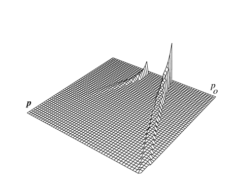
Figure 1: Spectral density for negative coupling.

Hence the energy needed to create a constituent particle of momentum ${\mbox{\boldmath$p$}}=0$ in the thermal background is equal to $m_{\sharp}$. It is larger than $m_{0}$ since one has to inject in addition to the rest mass of the particle its interaction energy with the thermal background. An analogous statement holds for the energy gained by the removal of a particle from the state (creation of a hole). For non-zero momenta $p$, the mass shell of the particle, respectively hole, is spread over a region whose width increases with increasing temperature. A qualitative picture of the spectral density $\widetilde{\rho}_{-}$ is given in Fig. 1.

The spectral density vanishes for large spacelike momenta, hence the state complies with the relativistic KMS condition (which can also be seen directly from Eq. (4.6)). It thus has all properties, outlined in [14], which are expected to be characteristic for the dissipative propagation of the constituents of a thermal state. By similar elementary computations, one can also determine the Fourier transforms of the time-ordered, retarded and advanced two-point functions from the correlation function (4.6); this is done for completeness in Appendix B.

Let us determine now the asymptotic thermal correlation functions for a quartic interaction with positive coupling $g>0$. There one might be inclined to replace in the two-point function (4.6) the sine by its hyperbolic counterpart. Yet the resulting function is not temperate and does not give rise to a state on ${\cal A}_{0}$. This apparent problem is solved by noticing that the regularity assumptions, made for the functions ${\langle\,Z({\mbox{\boldmath$x$}})\,\rangle_{0,\beta}}$ in the previous section for simplicity, are no longer valid in this case. In fact, one may impose Eq. (4.4) only for ${\mbox{\boldmath$x$}}\neq 0$, and the physically acceptable solutions are given by

$${\langle\,Z({\mbox{\boldmath$x$}})\,\rangle_{0,\beta}}=\mbox{const}\ {e^{-\mbox{\footnotesize$\kappa(\beta)$}\,|\mbox{\footnotesize\boldmath$x$}|}\over|{\mbox{\boldmath$x$}}|}.$$ (4.9)

It is instructive to discuss in a more systematic manner how these solutions arise. To this end we have to reconsider the definition of the normal-ordered cube of the field $\phi_{0}$ in situations where the functions ${\langle\,Z({\mbox{\boldmath$x$}})\,\rangle_{0,\beta}}$ exhibit a singularity at ${\mbox{\boldmath$x$}}=0$. Keeping $\varepsilon>0$ fixed for a moment, we define the regularized cube

$$\phi_{0}^{3}(x\,;\varepsilon)$$ (4.10)

$$=\phi_{0}(x+{\mbox{\boldmath$\varepsilon$}}_{1})\phi_{0}(x+{\mbox{\boldmath$\varepsilon$}}_{2})\phi_{0}(x+{\mbox{\boldmath$\varepsilon$}}_{3})-\!\sum{\langle\,\phi_{0}(x+{\mbox{\boldmath$\varepsilon$}}_{j})\,\phi_{0}(x+{\mbox{\boldmath$\varepsilon$}}_{k})\,\rangle_{0,\infty}}\,\phi_{0}(x+{\mbox{\boldmath$\varepsilon$}}_{l}),$$

where the spatial vectors ${\mbox{\boldmath$\varepsilon$}}_{j}$, $j=1,2,3$, form the corners of an equilateral triangle of side length $\varepsilon$ with $0$ at its barycenter and the sum extends over all partitions of $\{1,2,3\}$ into an ordered pair and a singlet. Replacing the expression given in (4.1) by its regularized version

$$N_{\varepsilon}(x)={1/3}\,\sum_{j=1}^{3}\big{(}\square\,\phi_{0}(x+{\mbox{\boldmath$\varepsilon$}}_{j})+m_{0}^{2}\,\phi_{0}(x+{\mbox{\boldmath$\varepsilon$}}_{j})\big{)}+g\,\phi_{0}^{3}(x\,;\varepsilon),$$ (4.11)

we demand as before that the admissible KMS states satisfy the corresponding compatibility condition (3.19) at non-singular points. In particular,

$$\lim_{x_{0}\rightarrow\infty}\,x_{0}^{3/2}\,{\langle\,N_{\varepsilon}(x)\,\phi_{0}(0)\,\rangle_{0,\beta}}=0$$ (4.12)

for $|{\mbox{\boldmath$x$}}|>\varepsilon$. Restricting as before our attention to isotropic KMS states satisfying the normalization condition ${\langle\,Z({\mbox{\boldmath$\varepsilon$}})\,\rangle_{0,\beta}}=1$ for $|{\mbox{\boldmath$\varepsilon$}}|=\varepsilon$, this condition is fulfilled provided ${\langle\,Z({\mbox{\boldmath$x$}})\,\rangle_{0,\beta}}$ is, for ${\mbox{\boldmath$x$}}\neq 0$, a solution of

$$(-\Delta+3gk_{\varepsilon}(\beta))\,{\langle\,Z({\mbox{\boldmath$x$}})\,\rangle_{0,\beta}}=0,$$ (4.13)

where

$$k_{\varepsilon}(\beta)=2\,(2\pi)^{-3}\int\!dp\ \theta(p_{0})\delta(p^{2}-m_{0}^{2})\,(e^{\beta p_{0}}-1)^{-1}\,\cos({\mbox{\boldmath$p$}}{\mbox{\boldmath$\varepsilon$}}).$$ (4.14)

The temperate, isotropic and normalized solutions are

$${\langle\,Z({\mbox{\boldmath$x$}})\,\rangle_{0,\beta}}=\varepsilon\,e^{\,\mbox{\footnotesize$\kappa_{\varepsilon}(\beta)$}\mbox{\footnotesize\boldmath$\varepsilon$}}\ \,{e^{-\mbox{\footnotesize$\kappa_{\varepsilon}(\beta)$}\,|\mbox{\footnotesize\boldmath$x$}|}\over|{\mbox{\boldmath$x$}}|},$$ (4.15)

where $\kappa_{\varepsilon}(\beta)=(3\,g\,k_{\varepsilon}(\beta))^{1/2}$. They fix the KMS states which are asymptotically compatible with the regularized interaction.

In order to obtain a meaningful result in the limit $\varepsilon\rightarrow 0$, one has to renormalize the field $\phi_{0}$ by the temperature independent factor $(\kappa_{0}\,\varepsilon)^{-1/2}$, $\kappa_{0}$ being some fixed energy, so as to compensate the factor $\varepsilon$ in (4.15). Since $\kappa_{\varepsilon}(\beta)\rightarrow\kappa(\beta)$ for $\varepsilon\rightarrow 0$, the two-point functions of the renormalized field arising in this limit are

$${\langle\,\phi_{0}(x_{1})\phi_{0}(x_{2})\,\rangle_{0,\beta}}={e^{-\mbox{\footnotesize$\kappa(\beta)$}\,|\mbox{\footnotesize\boldmath${\mbox{\boldmath$x$}}_{1}-{\mbox{\boldmath$x$}}_{2}$}|}\over\kappa_{0}\,|{\mbox{\boldmath$x$}}_{1}-{\mbox{\boldmath$x$}}_{2}|}\ W_{m_{0},\beta}(x_{1}-x_{2}).$$ (4.16)

These functions exhibit a universal singular behaviour at coinciding arguments which may be attributed to the bad ultraviolet properties of the quartic interaction for positive couplings. In particular, the field no longer satisfies canonical equal time commutation relations in the thermal states. Moreover, the two-point functions do not converge to the thermal correlation functions of a non-interacting field for $g\searrow 0$. They also do not approach the vacuum situation in the limit of zero temperature, but define a ground state. So the physical situation described by these functions is quite different from that for negative coupling.

The momentum space spectral density of the two-point function (4.16) is given by the following expression (see also the corresponding Green’s function in Appendix B):

$$\widetilde{\rho}_{+}(p)={1\over 1\!-\!e^{-\beta p_{0}}}\ {\varepsilon(p_{0})\over 8\pi^{2}\kappa_{0}|{\mbox{\boldmath$p$}}|}\ \theta(p_{0}^{2}\!-\!m_{0}^{2})\ \ln{\big{(}(p_{0}^{2}-m_{0}^{2})^{1/2}+|{\mbox{\boldmath$p$}}|\big{)}^{2}+\kappa(\beta)^{2}\over\big{(}(p_{0}^{2}-m_{0}^{2})^{1/2}-|{\mbox{\boldmath$p$}}|\big{)}^{2}+\kappa(\beta)^{2}}.$$ (4.17)

It is again non-negative, so also in the case of positive coupling there exist thermal states on the algebra of asymptotic thermal fields which are compatible with the asymptotic dynamics. But these states no longer comply with the relativistic KMS condition due to their singular behaviour in configuration space.

In contrast to the previous case, the support of the density $\widetilde{\rho}_{+}$ is now spread over the whole region $|p_{0}|\geq m_{0}$. It has, for small temperatures, sharp maxima in $p_{0}$ for given $|{\mbox{\boldmath$p$}}|$ which define approximate dispersion laws for the constituent particles and the corresponding holes in the thermal background. Again, one has to inject an energy of order $m_{\sharp}$ in order to create with substantial probability a particle of zero momentum in the thermal background. In Fig. 2 a qualitative picture of the spectral density $\widetilde{\rho}_{+}$ is given for the same mass, modulus of the coupling constant, temperature and range of momenta as in Fig. 1.

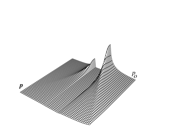
Figure 2: Spectral density for positive coupling.

The preceding results show that the algebra of asymptotic thermal fields and the concept of asymptotic field equations provides an efficient tool for the non-perturbative computation of the asymptotic thermal propagators. These propagators can be computed in a straight-forward manner from the underlying field equations in which the physical mass $m_{0}$ of the particle and strength $g$ of the interaction are encoded. We mention as an aside that in the perturbative computation of thermal Green’s functions these parameters can be fixed independently of the temperature [17].

Since there did not appear any inconsistencies in the present asymptotic analysis, there arises the interesting question of whether also the full theory with a quartic interaction can be defined in thermal states, in contrast to the vacuum, where it is expected to be trivial for positive couplings and unstable for negative ones. The preceding results seem to indicate that free field theory would not be the appropriate starting point, however, for the construction if $g>0$. One should start instead from a theory, where the specific short distance structure of the propagators is taken into account from the outset. This is in accordance with the ideas expounded in [18] which may be of relevance also in the present context.

5 Conclusions

Starting from general physical assumptions, we have determined the asymptotic form of the thermal correlation functions of scalar fields. It turned out that discrete mass contributions in the Källén-Lehmann type representation of the two-point functions give rise to asymptotically leading terms which have a rather simple form: they are products of the thermal correlation function of a free field and a damping factor describing the dissipative effects of the model-dependent thermal background.

The asymptotic correlation functions can be interpreted in terms of quasifree states on some central extension of the algebra of a free scalar field. Intuitively speaking, this field carries an additional stochastic degree of freedom which manifests itself in a central element appearing in the commutation relations and couples to the thermal backgrounds. In thermal states describing pure phases, this central element “freezes” in the sense that it attains sharp c-number values, whereas in mixtures of such states it is statistically fluctuating.

The concrete examples of two-point functions computed in the present investigation nicely illustrate the conclusions of the general discussion in [14]. They corroborate the idea that the stable “constituent particles” forming a thermal state give rise to discrete mass contributions in the damping factors. The existence of such discrete contributions has also been established in the presence of spontaneous symmetry breaking [19], where they can be attributed to the appearance of Goldstone Bosons. All these results provide evidence to the effect that the constituents of thermal states produce an unambiguous signal in the correlation functions in configuration space. It is not so easy, however, to discriminate them in momentum space from other types of excitations since the damping factors wipe out their discrete mass shells.

It is apparent that the present non-perturbative method for the analysis and computation of the asymptotic form of the thermal correlation functions can be extended to theories with a more complex field content. There appears, however, a technical problem in the treatment of fields affiliated with massless particles. In order to identify their asymptotically leading contribution in the thermal correlation functions one needs a more refined analysis which allows one to distinguish the effects of massless constituent particles from those of collective low-energy excitations. We hope to return to this interesting problem elsewhere.

Appendix A Asymptotic behaviour of free propagators

In this appendix we establish asymptotic bounds on the smeared–out free thermal correlation functions, used in Sec. 2, which are uniform in the mass. Let $h\in{\cal S}(\mathbb{R})$ be any test function whose Fourier transform vanishes at the origin. We consider the functions, $x$ varying in compact sets and $x_{0}$ being positive,

$$x_{0} \rightarrow \int\!dp\,\varepsilon(p_{0})\delta(p^{2}-m^{2})\,(1-e^{-{\mbox{\footnotesize$\beta$}}{\mbox{\footnotesize$p_{0}$}}})^{-1}\,\widetilde{h}(p_{0})\,{\mbox{\boldmath$p$}}^{{\mbox{\footnotesize\boldmath$\mu$}}}\,e^{{\mbox{\footnotesize$i$}}({\mbox{\footnotesize$p_{0}$}}{\mbox{\footnotesize$x_{0}$}}-{\mbox{\footnotesize\boldmath$p$}}{\mbox{\footnotesize\boldmath$x$}})}$$ (A.1)

$$= \sum_{{\mbox{\footnotesize$\sigma$}}=\pm}\sigma\int\!{d{\mbox{\boldmath$p$}}\over 2\omega}\,(1-e^{-{\mbox{\footnotesize$\sigma$}}{\mbox{\footnotesize$\beta$}}{\mbox{\footnotesize$\omega$}}})^{-1}\,\widetilde{h}(\sigma\omega)\,{\mbox{\boldmath$p$}}^{{\mbox{\footnotesize\boldmath$\mu$}}}\,e^{{\mbox{\footnotesize$i$}}({\mbox{\footnotesize$\sigma$}}{\mbox{\footnotesize$x_{0}$}}{\mbox{\footnotesize$\omega$}}-{\mbox{\footnotesize\boldmath$x$}}{\mbox{\footnotesize\boldmath$p$}})},$$

where $\omega=({\mbox{\boldmath$p$}}^{2}+m^{2})^{1/2}$ and ${\mbox{\boldmath$p$}}^{{\mbox{\footnotesize\boldmath$\mu$}}}=p_{1}^{\mu_{1}}p_{2}^{\mu_{2}}p_{3}^{\mu_{3}}$ is any given monomial in the components of $p$ of degree $\mu=\sum_{j}\mu_{j}$. Performing the spherical integration and making the substitution $w=(\omega-m)/x_{0}$, we can proceed to

$$=\ \ \sum_{{\mbox{\footnotesize$\sigma$}}=\pm}e^{{\mbox{\footnotesize$i$}}{\mbox{\footnotesize$\sigma$}}{\mbox{\footnotesize$m$}}{\mbox{\footnotesize$x_{0}$}}}x_{0}^{-(\mu+3)/2}\int_{0}^{\infty}\!dw\,e^{{\mbox{\footnotesize$i$}}{\mbox{\footnotesize$\sigma$}}{\mbox{\footnotesize$w$}}}\,w^{(\mu+1)/2}\,k_{\sigma}(w/x_{0};m),$$ (A.2)

where

$$\begin{split}k_{\sigma}(v;m)&=\sigma\,(v+2m)^{(\mu+1)/2}\,(1-e^{-{\mbox{\footnotesize$\sigma$}}{\mbox{\footnotesize$\beta$}}({\mbox{\footnotesize$v$}}+{\mbox{\footnotesize$m$}})})^{-1}\,\widetilde{h}(\sigma(v+m))\\ &\times\int\!d\,\Omega({\mbox{\boldmath$e$}})\,e^{-{\mbox{\footnotesize$i$}}({\mbox{\footnotesize$v$}}^{2}+2{\mbox{\footnotesize$m$}}{\mbox{\footnotesize$v$}})^{1/2}{\mbox{\footnotesize\boldmath$x$}}{\mbox{\footnotesize\boldmath$e$}}}\,{\mbox{\boldmath$e$}}^{\mbox{\footnotesize\boldmath$\mu$}}\end{split}$$ (A.3)

and $d\,\Omega({\mbox{\boldmath$e$}})$ denotes the measure on the unit sphere $|{\mbox{\boldmath$e$}}|=1$. Since $\widetilde{h}(0)=0$, the latter functions are, for fixed $m\geq 0$, continuous and rapidly decreasing in $v$. Moreover, since $\widetilde{h}$ is a test function, we obtain for fixed $0<\delta<1/2$ and $n\in\mathbb{N}$ bounds on the $n$-fold derivative of $k_{\sigma}$ of the form

$$\sup_{v>0}|v^{n-\delta}\,\partial_{v}^{\,n}\,k_{\sigma}(v;m)|\leq c_{N}\,(1+m)^{-N},$$ (A.4)

which hold uniformly on compact sets in $x$ and for any $N\in\mathbb{N}$. It is an immediate consequence of this estimate that

$$|k_{\sigma}(v;m)-k_{\sigma}(0;m)|\leq\delta^{-1}v^{\delta}\,\sup_{u>0}|u^{1-\delta}\,\partial_{u}\,k_{\sigma}(u;m)|\leq c_{N}\,v^{\delta}(1+m)^{-N}.$$ (A.5)

We now split the integral in (A.2) into

$$\begin{split}&k_{\sigma}(0;m)\,\lim_{\varepsilon\searrow 0}\,\int_{0}^{\infty}\!dw\,e^{{\mbox{\footnotesize$i$}}{\mbox{\footnotesize$\sigma$}}{\mbox{\footnotesize$w$}}-{\mbox{\footnotesize$\varepsilon$}}{\mbox{\footnotesize$w$}}}\,w^{(\mu+1)/2}\\ &+\lim_{\varepsilon\searrow 0}\,\int_{0}^{\infty}\!dw\,e^{{\mbox{\footnotesize$i$}}{\mbox{\footnotesize$\sigma$}}{\mbox{\footnotesize$w$}}-{\mbox{\footnotesize$\varepsilon$}}{\mbox{\footnotesize$w$}}}\,w^{(\mu+1)/2}\,(k_{\sigma}(w/x_{0};m)-k_{\sigma}(0;m)).\end{split}$$ (A.6)

The first term is a continuous, rapidly decreasing function of $m$. For the modulus of the second term we obtain by $\nu$-fold partial integration, $(\mu+3)/2<\nu\leq(\mu+5)/2$, an upper bound of the form

$$\begin{split}&\Big{|}\int_{0}^{\infty}\!dw\,(e^{{\mbox{\footnotesize$i$}}{\mbox{\footnotesize$\sigma$}}{\mbox{\footnotesize$w$}}-{\mbox{\footnotesize$\varepsilon$}}{\mbox{\footnotesize$w$}}}-1)\,w^{(\mu+1)/2-\nu}\,\sum_{n=0}^{\nu}c_{n}\,(w/x_{0})^{n}\,(\partial^{n}k_{\sigma})(w/x_{0};m)\Big{|}\\ &\leq c_{N}\,|x_{0}|^{-\delta}\,(1+m)^{-N}\,\int_{0}^{\infty}\!dw\,|e^{{\mbox{\footnotesize$i$}}{\mbox{\footnotesize$\sigma$}}{\mbox{\footnotesize$w$}}-{\mbox{\footnotesize$\varepsilon$}}{\mbox{\footnotesize$w$}}}-1|\,w^{(\mu+1)/2-\nu+\delta},\end{split}$$ (A.7)

where $(\partial^{0}k_{\sigma})(v;m)\doteq k_{\sigma}(v;m)-k_{\sigma}(0;m)$ and we made use of the bounds (A.4) and (A.5). As $1<\nu-(\mu+1)/2-\delta<2$, the latter integral exists and converges in the limit $\varepsilon\searrow 0$. So, to summarize, we find that there holds

$$h*\partial^{\mbox{\footnotesize\boldmath$\mu$}}_{\mbox{\footnotesize\boldmath$x$}}\,{W_{m,\beta}}(x)=x_{0}^{-(\mu+3)/2}\big{(}e^{-imx_{0}}k_{+}(m)+e^{imx_{0}}k_{-}(m)\big{)}+r(m,x),$$ (A.8)

where $k_{\pm}(m)$ are continuous functions which decrease faster than any inverse power of $m$ in the limit of large $m$. The remainder $r(m,x)$ is continuous in $m$ and bounded by

$$|r(m,x)|\leq c_{N}\,x_{0}^{-(\mu+3)/2-\delta}\,(1+m)^{-N},$$ (A.9)

uniformly on compact sets in $x$. By similar arguments one obtains an analogous result for large negative $x_{0}$. We note in conclusion that the preceding statements hold for fixed mass $m>0$ also without the time-smearing by the test function $h$.

Appendix B Asymptotic thermal Green’s functions

In the main text we have focussed our attention on the correlation functions of the thermal fields. As the standard real and imaginary time formalisms of thermal quantum field theory are based on the time-ordered, respectively retarded and advanced functions, we translate here our results into these perhaps more familiar settings. We begin by recalling the relations between these functions and then turn to the concrete examples discussed in Sec. 5.

Taking into account the anticipated invariance of the thermal states under space-time translations, the thermal correlation functions

$$W(x_{1}-x_{2})\doteq{\langle\,\phi(x_{1})\phi(x_{2})\,\rangle_{\beta}}$$ (B.1)

fix the commutator function $C$ by the formula

$$C(x)=W(x)-W(-x).$$ (B.2)

Because of locality, $C$ has support in the union of the closed forward and backward lightcones $\overline{V}^{\pm}$. The retarded and advanced functions $R$, $A$ have support in $\overline{V}^{+}$ and $\overline{V}^{-}$, respectively, and are obtained by splitting $i\,C$ into

$$i\,C(x)=R(x)-A(x),$$ (B.3)

the factor $i$ being a matter of convention. In the cases of interest here, this splitting can be performed without ambiguities in view of the mild singularities of $C$ at the origin. The time-ordered and anti-time-ordered functions $T$ and $\overline{T}$, respectively, are obtained by setting

$$T(x) = W(x)-iA(x)=W(-x)-iR(x)$$ (B.4)

$${\overline{T}}(x) = W(x)+iR(x)=W(-x)+iA(x).$$ (B.5)

We now pass to Fourier-space. It is an interesting feature of the asymptotic thermal fields considered in Sec. 4 that the Fourier transforms $\widetilde{C}$ of the thermal commutator functions vanish in the region ${\cal{R}}_{m_{0}}=\{p\in\mathbb{R}^{4}:|p_{0}|<m_{0}\}$, cf. the examples considered in Sec. 5. In this situation one can establish the existence of Green’s functions $\widetilde{G}$ which are analytic in momentum space by the following standard argument: The Fourier transforms $\widetilde{R}$, $\widetilde{A}$ of the retarded and advanced functions can be extended analytically into the forward and backward tubes ${\cal{T}}^{\pm}=\{k\in\mathbb{C}^{\,4}:\mbox{Im}\,k\in V^{\pm}\}$, respectively, because of their support properties in configuration space. Moreover, from the momentum space version of (B.3),

$$\widetilde{R}(p)-\widetilde{A}(p)=i\,\widetilde{C}(p),$$ (B.6)

one sees that $\widetilde{R}$ and $\widetilde{A}$ coincide on ${\cal{R}}_{m_{0}}$. It thus follows from the Edge-of-the-Wedge theorem that $\widetilde{R}$, $\widetilde{A}$ are pieces of an analytic function $\widetilde{G}$, the Green’s function, with domain of holomorphy containing ${\cal{T}}^{+}\cup{\cal{T}}^{-}\cup{\cal{R}}_{m_{0}}.$ In particular, there holds the discontinuity formula

$$\lim_{\varepsilon\searrow 0}\widetilde{G}(p_{0}+i\varepsilon,{\mbox{\boldmath$p$}})-\lim_{\varepsilon\searrow 0}\widetilde{G}(p_{0}-i\varepsilon,{\mbox{\boldmath$p$}})=i\widetilde{C}(p).$$ (B.7)

For real spatial momenta $p$, the Green’s function $\widetilde{G}$ can thus be obtained by the Cauchy integral (or dispersion relation) on the twofold cut complex $k_{0}$-plane,

$$\widetilde{G}(k_{0},{\mbox{\boldmath$p$}})={1\over 2\pi}\ \int dp_{0}\ {{\widetilde{C}}(p_{0},{\mbox{\boldmath$p$}})\over p_{0}-k_{0}}.$$ (B.8)

Although this formula does not exhibit by itself the analytic continuation of $\widetilde{G}$ in all momentum space variables, it is of practical use for computations in the specific examples treated below. Moreover, since $p_{0}\,\widetilde{C}(p)$ is positive as a consequence of the KMS condition and the positivity of $\widetilde{W}(p)$, it shows that $\widetilde{G}(p)$ is positive on the coincidence region ${\cal R}_{m_{0}}$. The latter property distinguishes the restriction of the analytic Green’s function to its physical-sheet domain based on ${\cal{T}}^{+}\cup{\cal{T}}^{-}\cup{\cal{R}}_{m_{0}}$.

The Fourier transforms of the (anti) time-ordered functions are given in terms of ${\widetilde{R}}$ and ${\widetilde{A}}$ (and hence in terms of the boundary values of $\widetilde{G}$) by the formulas

$$\widetilde{T}(p) = i\,{\widetilde{A}(p)-\widetilde{R}(p)\over 1-e^{-\beta p_{0}}}-i\,{\widetilde{A}(p)}$$ (B.9)

$$\widetilde{\overline{T}}(p) = i\,{\widetilde{A}(p)-\widetilde{R}(p)\over 1-e^{-\beta p_{0}}}+i\,{\widetilde{R}(p)}.$$ (B.10)

We note that in the region of coincidence ${\cal R}_{m_{0}}$ these equations reduce (as in the vacuum case) to

$${\widetilde{G}}(p)={\widetilde{R}}(p)={\widetilde{A}}(p)=i\widetilde{T}(p)=-i\widetilde{\overline{T}}(p).$$ (B.11)

After these preliminaries, we can now turn to the two concrete examples treated in Sec. 5. In view of the preceding formulas, relating the functions of interest to the Green’s function in a straightforward manner, it suffices to determine the latter.

In the case of negative coupling, $g<0$, the Fourier transform of the commutator function, i.e. the spectral function, is the odd part of the spectral density (4.7), multiplied by $2$. Thus it is given by

$$\widetilde{C}_{-}(p_{0},{\mbox{\boldmath$p$}})={\varepsilon(p_{0})\over 8\pi\kappa(\beta)|{\mbox{\boldmath$p$}}|}\,\theta(p^{2}\!-\!m_{\sharp}^{2}\!+\!2\kappa(\beta)|{\mbox{\boldmath$p$}}|)\ \theta(-p^{2}\!+\!m_{\sharp}^{2}\!+\!2\kappa(\beta)|{\mbox{\boldmath$p$}}|),$$ (B.12)

where $m_{\sharp}^{2}=m_{0}^{2}+\kappa(\beta)^{2}$. By performing the above Cauchy integral one obtains the corresponding Green’s function for complex $(k_{0},{\mbox{\boldmath$k$}})$,

$$\widetilde{G}_{-}(k_{0},{\mbox{\boldmath$k$}})={1\over 16\pi^{2}\kappa(\beta)({\mbox{\boldmath$k$}}^{2})^{1/2}}\,\ln{k^{2}\!-\!m_{\sharp}^{2}\!-\!2\kappa(\beta)({\mbox{\boldmath$k$}}^{2})^{1/2}\over k^{2}\!-\!m_{\sharp}^{2}\!+\!2\kappa(\beta)({\mbox{\boldmath$k$}}^{2})^{1/2}},$$ (B.13)

where the principal (positive) branch of the logarithm and $({\mbox{\boldmath$p$}}^{2})^{1/2}=|{\mbox{\boldmath$p$}}|$ have to be chosen in the region ${\cal R}_{m_{0}}$ of the physical sheet in view of the above positivity constraint on $\widetilde{G}_{-}$. The logarithmic singularity of this holomorphic function is carried by the complex hypersurface $\Sigma_{\sharp}$ with equation $(k^{2}-m_{\sharp}^{2})^{2}-4\kappa(\beta)^{2}{\mbox{\boldmath$k$}}^{2}=0$ which can explicitly be seen not to intersect the domains $\cal{T}^{+}$ and $\cal{T}^{-}$, while its trace on the reals is the border of the region described by (4.8). The set with equation ${\mbox{\boldmath$k$}}^{2}=0$ does not carry singularity in the physical sheet and at ${\mbox{\boldmath$k$}}=0$ one obtains

$$\widetilde{G}_{-}(k_{0},0)=-{1\over 4\pi^{2}}\,{1\over k_{0}^{2}\ -\ m_{\sharp}^{2}}.$$ (B.14)

The retarded, advanced and (anti) time-ordered functions are obtained from $\widetilde{G}_{-}$ by the preceding formulas. We note that the coincidence relation (B.11) holds not only on ${\cal R}_{m_{0}}$, but everywhere in the complement of the region (4.8), yielding an extended physical sheet domain for $\widetilde{G}_{-}$.

Turning to the case of positive coupling, $g>0$, we see from relation (4.17) that the corresponding commutator (spectral) function is equal to

$$\widetilde{C}_{+}(p_{0},{\mbox{\boldmath$p$}})={\varepsilon(p_{0})\over 8\pi^{2}\kappa_{0}\,|{\mbox{\boldmath$p$}}|}\,\theta(p_{0}^{2}\!-\!m_{0}^{2})\,\ln{\big{(}(p_{0}^{2}-m_{0}^{2})^{1/2}+|{\mbox{\boldmath$p$}}|\big{)}^{2}+\kappa(\beta)^{2}\over\big{(}(p_{0}^{2}-m_{0}^{2})^{1/2}-|{\mbox{\boldmath$p$}}|\big{)}^{2}+\kappa(\beta)^{2}}.$$ (B.15)

Inserting this function into (B.8), splitting the logarithm into two parts and making a contour-distortion argument now yields the analytic Green’s function

$$\widetilde{G}_{+}(k_{0},{\mbox{\boldmath$k$}})={i\over 8\pi^{2}\kappa_{0}\,({\mbox{\boldmath$k$}}^{2})^{1/2}}\,\ln{(k_{0}^{2}-m_{0}^{2})^{1/2}+({\mbox{\boldmath$k$}}^{2})^{1/2}+i\kappa(\beta)\over(k_{0}^{2}-m_{0}^{2})^{1/2}-({\mbox{\boldmath$k$}}^{2})^{1/2}+i\kappa(\beta)},$$ (B.16)

where in the region ${\cal R}_{m_{0}}$ one has to choose again the principal branch of the logarithm, $({\mbox{\boldmath$p$}}^{2})^{1/2}=|{\mbox{\boldmath$p$}}|$ and $(p_{0}^{2}-m_{0}^{2})^{1/2}=i\,|p_{0}^{2}-m_{0}^{2}|^{1/2}$.

The logarithmic singularity of $\widetilde{G}_{-}$ is now carried by the complex hypersurface $\Sigma_{\flat}$ with equation $(k^{2}-m_{\flat}^{2})^{2}+4\kappa(\beta)^{2}{\mbox{\boldmath$k$}}^{2}=0$, where $m_{\flat}^{2}=m_{0}^{2}-\kappa(\beta)^{2}$. In contrast to $\Sigma_{\sharp}$, the surface $\Sigma_{\flat}$ intersects the domains $\cal{T}^{\pm}$, but the corresponding points appear as singularities of $\widetilde{G}_{+}$ only in unphysical sheets. If $m_{\flat}^{2}$ is negative, i.e. at large temperatures, $\Sigma_{\flat}$ does not contain any real points. For low temperatures the only real points of $\Sigma_{\flat}$ are $\pm(m_{\flat},{\mbox{\boldmath$0$}})$; they appear as second sheet singularities (“anti-boundstates”), cf. Eq. (B.17) below.

On the real border of its physical sheet domain, the only singularity of $\widetilde{G}_{+}$ is the square-root type threshold singularity at $p_{0}=\pm m_{0}$ for all $p$ since, here again, the set with equation ${\mbox{\boldmath$k$}}^{2}=0$ does not carry singularity in the physical sheet. At ${\mbox{\boldmath$k$}}=0$, one obtains

$$\widetilde{G}_{+}(k_{0},0)={i\over 4\pi^{2}\kappa_{0}}\ {1\over(k_{0}^{2}-m_{0}^{2})^{1/2}+i\kappa(\beta)}.$$ (B.17)

The retarded and advanced functions, defined in terms of the corresponding boundary values of $\widetilde{G}_{+}$, and the (anti) time-ordered functions given by relation (B.9) now satisfy the coincidence relation (B.11) only in the region ${\cal R}_{m_{0}}$.

Acknowledgements
The authors are grateful for hospitality and financial support by the Universität Göttingen and the CEA - Saclay, respectively.

References

• [1] H. Narnhofer, M. Requardt and W. Thirring, Commun. Math. Phys.  92, 247 (1983).
• [2] N.P. Landsman, Annals Phys.  186, 141 (1988).
• [3] O. Steinmann, Commun. Math. Phys.  170, 405 (1995)
• [4] H.A. Weldon, Quasiparticles in finite-temperature field theory, preprint hep-ph/9809330
• [5] A. A. Abrikosov, Phys. Atom. Nucl. 59, 352 (1996) (from Yad. Fiz. 59N2, 372 (1996))
• [6] E. Braaten and R.D. Pisarski, Nucl. Phys. B 337, 569 (1990).
• [7] J.P. Blaizot and E. Iancu, Phys. Rev. D 55, 973 (1997); 56, 7877 (1997).
• [8] M. Le Bellac, Thermal Field Theory. Cambridge University Press, Cambridge, England, 1996.
• [9] P. Arnold and L.G. Yaffe, Phys. Rev. D 57, 1178 (1998)
• [10] J. Bros and D. Buchholz, Annales Poincaré Phys. Theor.  64, 495 (1996)
• [11] N. P. Landsman and C. G. van Weert, Phys. Rept.  145, 141 (1987)
• [12] L. Dolan and R. Jackiw, Phys. Rev. D 9, 3320 (1974).
• [13] J. Bros and D. Buchholz, Nucl. Phys. B 429, 291 (1994)
• [14] J. Bros and D. Buchholz, Z. Phys. C 55, 509 (1992).
• [15] H.A. Weldon, Asymptotic space-time behaviour of HTL gauge propagator, preprint hep-ph/0009240.
• [16] K. Symanzik, Commun. Math. Phys.  18, 227 (1970) and Commun. Math. Phys.  23, 49 (1971).
• [17] C. Kopper, V.F. Müller and T. Reisz, Annales Henri Poincaré 2, 387 (2001)
• [18] J.R. Klauder, Self-interacting scalar fields and (non-)triviality, p. 87 in: Mathematical Physics Towards the 21st Century. Proceedings Beer-Sheva 1993, R.N. Sen and A. Gersten Eds. Ben-Gurion University of the Negev Press, 1994
• [19] J. Bros and D. Buchholz, Phys. Rev. D 58, 125012 (1998)