Signatures of Doubly Charged Higgs Bosons in $e\gamma$ Collisions

Abstract

We study the discovery potential for doubly charged Higgs bosons, $\Delta^{--}$, in the process $e^{-}\gamma\to e^{+}\mu^{-}\mu^{-}$ for centre of mass energies appropriate to high energy $e^{+}e^{-}$ linear colliders and the CLIC proposal. For $M_{\Delta}<\sqrt{s_{e\gamma}}$ discovery is likely for even relatively small values of the Yukawa coupling to leptons. However, even far above threshold, evidence for the $\Delta$ can be seen due to contributions from virtual intermediate $\Delta$’s although, in this case, $\mu^{-}\mu^{-}$ final states can only be produced in sufficient numbers for discovery for relatively large values of the Yukawa couplings.

I Introduction

Doubly charged Higgs bosons arise in many extensions of the standard model (SM), typically as components of $SU(2)_{L}$ triplet representations. Although the single Higgs doublet adopted to break the SM gauge symmetry is the simplest possibility for the Higgs sector, the real nature of the Higgs sector is unknown and many other cases are worth consideration. A simple extension, which arises naturally in Supersymmetry, is to include two Higgs doublets. Beyond this, the introduction of a Higgs triplet is one of the next logical possibilities for the Higgs sector. While in the context of the SM there is no specific motivation for the introduction of a Higgs triplet there are several models which require a Higgs triplet for symmetry breaking. Perhaps the best known model with this requirement is the Left-Right symmetric model [1]. In this model the neutral scalar couplings to the fermions may also give rise to the see-saw mechanism leading to naturally small neutrino masses [2]. Another example of a model containing a Higgs triplet is the Left-handed Higgs triplet model of Gelmini and Roncadelli [3]. One of the consequences of a Higgs triplet with the appropriate quantum numbers is the existence of a doubly charged Higgs boson, the $\Delta^{--}$, which has a distinct experimental signature. Although the introduction of a Higgs triplet can introduce phenomenological difficulties it turns out that they are not difficult to avoid. Thus, the discovery of a $\Delta^{--}$ would have important implications for our understanding of the Higgs sector and more importantly, for what lies beyond the standard model.

There are a variety of processes sensitive to doubly charged Higgs bosons. Indirect constraints on masses and couplings have been obtained from lepton number violating processes and muonium-antimuonium conversion experiments [4, 5, 6, 7]. The most stringent limits come from that latter measurement [8, 4]. For flavour diagonal couplings these measurements require that the ratio of the Yukawa coupling, $h$, and Higgs mass, $M_{\Delta}$, satisfy $h/M_{\Delta}<0.44$ TeV^-1 at 90% C.L.. These bounds allow the existence of low-mass doubly charged Higgs with a small coupling constant. These limits can be circumvented in certain models as a result of cancellations among additional diagrams arising from other new physics [9, 10]. Thus, from this point of view, direct limits are generally more robust.

Search strategies for the $\Delta^{--}$ have been explored for the Fermilab Tevatron and the CERN Large Hadron Collider (LHC) [11, 12]. At the Tevatron it is expected that the doubly charged Higgs can be detected via pair production if its mass is less than $\sim 275$ GeV while at the LHC the reach extends to $\sim 850$ GeV, in both cases assuming a BR to leptons of 100% [11]. Signatures for the $\Delta^{--}$ have also been explored for high energy $e^{+}e^{-}$ colliders [13]. For the most part, limits obtained at $e^{+}e^{-}$ colliders have relied on $\Delta^{--}$ pair production so the mass reach is limited to $M_{\Delta}<\sqrt{s}/2$ although these can be exceeded by constraining t-channel $\Delta$ exchange in Bhabba scattering and single $\Delta^{--}$ production. Studies looking at doubly charged Higgs production in $e^{-}e^{-}$ colliders [9, 13, 14] find mass limits up to $\sqrt{s}$. There have been a number of studies of single $\Delta^{--}$ in $e\gamma$ [13, 15, 16, 17] collisions and also $e^{+}e^{-}$ and $\gamma\gamma$ collisions where in the latter cases the photon or electron is described using the effective photon or effective fermion approximation respectively [15]. In the case of $e\gamma$ collisions the kinematic limit is $\sim\sqrt{s_{e\gamma}}$. The most recent calculation by Gregores et al. [16], which most closely resembles the approach presented here, only included the Feynman diagrams with s-channel contributions from the $\Delta^{--}$ and therefore restricted their study to resonance $\Delta^{--}$ production. In effect they looked at $e^{-}e^{-}$ fusion where one of the $e^{-}$’s is the beam electron and the other arises from the equivalent particle approximation for an electron in the photon. In this approximation the authors assume that the positron is lost down the beam.

In this paper we study signals for doubly charged Higgs bosons in the process $e^{-}\gamma\to e^{+}\mu^{-}\mu^{-}$ including all contributions to the $e^{+}\mu^{-}\mu^{-}$ final state. We assume the photon is produced by backscattering a laser from the $e^{+}$ beam of an $e^{+}e^{-}$ collider [18]. We consider $e^{+}e^{-}$ centre of mass energies of $\sqrt{s}=500$, 800, 1000, and 1500 GeV appropriate to the TESLA/NLC/JLC high energy colliders [19, 20, 21] and $\sqrt{s}=3$, 5, and 8 TeV appropriate to the CLIC proposal [22]. In all cases we assume an integrated luminosity of ${\cal L}=500$ fb^-1. Our calculation includes diagrams which would not contribute to on-shell production of $\Delta^{--}$’s. Because the signature of same sign muon pairs in the final state is so distinctive and has no SM background, we find that the process can be sensitive to virtual $\Delta^{--}$’s with masses in excess of the centre of mass energy, depending on the strength of the Yukawa coupling to leptons.

In the next section we give a short overview of some models with doubly charged Higgs bosons and write down the Lagrangian describing their couplings to leptons. We also note some of the existing constraints on the relevant parameters of these models. In section III we describe our calculations and present our results. We conclude in section IV with some final comments.

II The models

In this section we give a brief description of the two most popular models with triplet Higgs bosons: The Left-handed Higgs Triplet Model (LHTM) and the Left-Right symmetric model (LRM). We mention only those aspects of the models which are of particular relevance to the process under consideration here. This, of course, includes the form of the Yukawa coupling of the triplet Higgs boson to fermions and we mention existing limits. We also consider the size of the possible vacuum expectation value of the neutral component of the triplet and include some discussion of the scalar mass spectrum of the models. All these parameters dictate which decay modes exist for the doubly charged Higgs and, consequently, its width. The process we consider is sensitive to the width of the $\Delta$ when $M_{\Delta}<\sqrt{s_{e\gamma}}$. All our results are applicable to both models.

The Left-handed Higgs Triplet model (LHTM) contains at least one Higgs triplet with weak hypercharge $Y=2$ which has lepton number violating couplings to leptons but does not couple to quarks. This triplet Higgs field was first introduced by Gelmini and Roncadelli [3] in order to give rise to Majorana masses for left-handed neutrinos while preserving $SU(2)_{L}$ gauge symmetry. The LHTM contains a Higgs triplet field in addition to all SM matter particles and the usual Higgs doublet. The minimal Higgs multiplet content of the model is thus [23]

$$\Delta=\left(\begin{array}[]{cc}\Delta^{-}/\sqrt{2}&\Delta^{--}\\ \Delta^{0}&-\Delta^{-}/\sqrt{2}\end{array}\right),\,\,\,\phi=\left(\begin{array}[]{c}\phi^{+}\\ \phi^{0}\end{array}\right).$$ (1)

Here the neutral components of the triplet and doublet multiplets may get vacuum expectation values (VEVs), denoted as $\langle\Delta^{0}\rangle=w/\sqrt{2}$ and $\langle\phi^{0}\rangle=v/\sqrt{2}$, respectively.

Isotriplet contributions to the masses of the electroweak bosons would result in a $\rho$-parameter, $\rho=(1+2x^{2})/(1+4x^{2})$ where $x=w/v$, in the LHTM which is less than unity even at tree level. As a result, the VEV, $w$, of the triplet Higgs is constrained to be small compared with the VEV, $v$, of the doublet. It is natural to be guided by the LEP II bound on the $\rho$ parameter [24]. The 3$\sigma$ LEP II bound corresponds to $w\sim 15$ GeV. Thus, we expect the value of the triplet’s VEV to be less than this and it may reasonably be set to zero; this is further justified below based on neutrino mass arguments.

The physical scalar particle content of the model is as follows: doubly charged Higgs $\Delta^{--}$, singly charged Higgs $H^{-}$ which are a mixture of the triplet and doublet components, and three neutral particles (two scalars and one pseudoscalar). The mixing in the neutral scalar sector is governed by the scalar potential, the most general form of which may be found in [23].

The Higgs potential of ref. [23] yields the following approximate relation between various scalar masses, valid in the limit $w\rightarrow 0$:

$$M_{\Delta^{--}}^{2}+M^{2}_{A}=2\cdot M_{H^{-}}^{2}$$ (2)

where $M_{A}$ is the pseudoscalar (pseudomajoron) mass. This relation implies that masses of doubly and singly charged Higgs particles should not differ too much (for reasonable Higgs self couplings). This has implications regarding the decay modes of the $\Delta^{--}$.

The triplet’s Yukawa coupling to lepton doublets is given by

$${\cal L}_{Yuk}=-ih_{ll^{\prime}}\Psi_{lL}^{T}C\sigma_{2}\Delta\Psi_{l^{\prime}L}+{h.c.},$$ (3)

where $C$ is the charge conjugation matrix and $\Psi_{lL}$ denotes the left-handed lepton doublet with flavour $l$.

This interaction (3) provides Majorana masses for neutrinos ($m_{\nu_{l}}=\sqrt{2}h_{ll}w$). The experimental upper bounds for the individual neutrino masses are $m_{\nu_{e}}\sim 2.3$ eV, $m_{\nu_{\mu}}\sim 170$ keV and $m_{\nu_{\tau}}\sim 18.2$ MeV [25]. Stronger yet is the bound on the sum over neutrino masses [26]

$$0.05<\sum_{i=e,\mu,\tau}m_{\nu_{i}}<8.4~{}eV.$$ (4)

The values of $h_{ll^{\prime}}$ and $w$ should be consistent with these limits, implying that, for Yukawa couplings in the range we are studying, the value $w$ should be of the order of the Majorana mass for left-handed neutrinos. This reinforces our assumption to neglect $w$.

Of course, the left-handed chirality of the Higgs triplet is not something immutable. However, a reasonable theory with natural right-handed Higgs triplet requires extended gauge symmetry.

The Left-Right Symmetric Model, based on the gauge symmetry $SU(2)_{L}\times SU(2)_{R}\times U(1)_{B-L}$, treats left-handed and right-handed fermions symmetrically. That is, left-handed fermion fields transform as doublets under $SU(2)_{L}$ and as singlets under $SU(2)_{R}$, while the reverse is true for right-handed fermions [1]. The fermionic sector contains, in addition to SM particles, a right-handed neutrino for each family. The extension of the gauge symmetry also brings new (right-handed ) gauge bosons $W_{R}$ and $Z_{R}$ into the model.

The scalar sector of the LR model contains many more degrees of freedom than in the SM. Rather than the standard Higgs doublet, it includes a scalar bidoublet $\Phi$ with the quantum numbers $({2},{2}^{*},0)$; $\Phi$ gives rise to fermion Dirac masses and breaks the SM gauge symmetry to $U(1)_{em}$. But, first, another Higgs field with non-vanishing $B-L$ is needed to break the gauge group $SU(2)_{L}\times SU(2)_{R}\times U(1)_{B-L}\,$ to the SM gauge symmetry. If one also wants to generate Majorana masses for the neutrino through the seesaw mechanism, a triplet Higgs field $\Delta_{R}$, with quantum numbers $(1,3,2)$ is required. Finally, for the case of explicit $L\leftrightarrow R$ symmetry, the corresponding left-handed triplet Higgs field should also be added:

$${\displaystyle\Delta_{L}=\left(\begin{array}[]{cc}\Delta_{L}^{-}/\sqrt{2}&\Delta_{L}^{--}\\ \Delta_{L}^{0}&-\Delta_{L}^{-}/\sqrt{2}\end{array}\right)=(3,1,2)}$$ (5)

For neutrino and gauge boson masses, the presence of the left-handed triplet Higgs is not essential. However, we will focus our attention on this representation. The $\rho$-parameter constraints on a possible VEV for its neutral component, $v_{L}/\sqrt{2}$, hold as described above.

The most general potential describing the self-interactions of the scalar fields introduced above can be found in, for example ref. [27]. There exist many phenomenological bounds on the parameters of this potential, only some of which are important here. In particular, the mass spectrum of the scalar sector is determined by the scalar potential. It is important to note that the doubly charged Higgs triplets remain practically unmixed [28] under our assumption that the VEV of $\Delta_{L}$ is negligible. At the same time this assumption again leads to the relationship of equation (2) for $\Delta_{L}^{--},\Delta_{L}^{-},\Delta_{L}^{A}$, although their masses in the LR model are no longer proportional to $v_{L}$. We will use these properties of the scalar mass spectrum in our calculations.

The Yukawa interactions of the Higgs triplets with fermions in the model read:

$$-{\cal L}_{Yuk}=ih_{R,ll^{\prime}}\Psi_{lR}^{T}C\sigma_{2}\Delta_{R}\Psi_{l^{\prime}R}+ih_{L,ll^{\prime}}\Psi_{{}^{\prime}L}^{T}C\sigma_{2}\Delta_{L}\Psi_{l^{\prime}L}\>\>\>+\>{\rm h.c.},$$ (6)

where $l,l^{\prime}$ are flavour indices. Along with the bidoublet’s Yukawa interactions, this yields the usual quark $3\times 3$ mass matrix and charged lepton masses, while for the neutrino one obtains a seesaw mass matrix. Of most relevance here is the constraint that left-handed neutrinos should be practically massless. This restricts the vacuum expectation value, $v_{L}$, of the neutral member of the Higgs triplet $\Delta_{L}$ to be small, as in our discussion of the LHTM above. Thus, it is possible to drop the effects of $v_{L}$ in our calculations.

The product of Yukawa couplings $h_{ee}h_{\mu\mu}$ dictates the magnitude of the process we consider here. Existing phenomenological constraints on $h_{ll^{\prime}}$ are as follows [4, 5, 6, 7]:

• The rare decays $\mu\rightarrow\bar{e}ee$ [29, 30] and $\mu\rightarrow e\gamma$ [31] yield very stringent restrictions on the non-diagonal couplings $h_{e\mu}$:

  $$h_{e\mu}h_{ee} < 3.2\times 10^{-11}\,{\rm GeV}^{-2}M_{\Delta}^{2},$$ (7)

  $$h_{e\mu}h_{\mu\mu} < 2\times 10^{-10}\,{\rm GeV}^{-2}M_{\Delta}^{2}.$$ (8)

  Consequently, we choose to neglect all non-diagonal couplings here.

• From Bhabha scattering one obtains the following upper limit for $h_{ee}$ [4],

  $$h_{ee}^{2}\sim 9.7\times 10^{-6}\,{\rm GeV}^{-2}M_{\Delta}^{2}.$$ (9)

• The $(g-2)_{\mu}$ measurement [32] provides an upper limit for $h_{\mu\mu}$,

  $$h_{\mu\mu}^{2}\sim 2.5\times 10^{-5}\,{\rm GeV}^{-2}M_{\Delta}^{2}.$$ (10)

• From muonium-antimuonium transition measurements one finds the following bound, which is the most stringent at present [8, 4, 6, 7]:

  $$h_{ee}h_{\mu\mu}\sim 2\times 10^{-7}\,{\rm GeV}^{-2}M_{\Delta}^{2}.$$ (11)

  The form of this bound, on the product $h_{ee}h_{\mu\mu}$, is directly relevant to the process we consider here.

• For the third generation Yukawa couplings $h_{\tau\tau}$, $h_{\tau e}$ and $h_{\tau\mu}$ there are no limits at present.

III Calculations and Results

We are studying the sensitivity to doubly charged Higgs bosons in the process $e^{-}\gamma\to e^{+}\mu^{-}\mu^{-}$. The signal of like-sign dimuons is distinct and SM background free, offering excellent potential for $\Delta^{--}$ discovery. The Feynman diagrams describing the direct production of doubly charged Higgs bosons are shown in Fig. 1a. Additionally, the non-resonant contributions of the Feynman diagrams of Fig. 1b contribute to the distinct $\mu^{-}\mu^{-}$ signal when $M_{\Delta}>\sqrt{s_{e\gamma}}$. These non-resonant contributions play an important role in the reach that one can obtain for doubly charged Higgs masses.

To calculate the cross section we must convolute the backscattered laser photon spectrum, $f_{\gamma/e}(x)$, with the subprocess cross section, $\hat{\sigma}(e^{-}\gamma\to e^{+}\mu^{-}\mu^{-})$;

$$\sigma=\int dxf_{\gamma/e}(x,\sqrt{s}/2)\;\hat{\sigma}(e^{-}\gamma\to e^{+}\mu^{-}\mu^{-}).$$ (12)

The backscattered photon spectrum is given in Ref. [18]. Beyond a certain laser energy $e^{+}e^{-}$ pairs are produced, which significantly degrades the photon beam. This leads to a maximum $e\gamma$ centre of mass energy of $\sim 0.91\times\sqrt{s}$.

We calculated the subprocess cross section with two different approaches as a cross-check of our results. In the first we obtained analytic expressions for the matrix elements using the CALKUL helicity amplitude method [33] and performed the phase space integrals using Monte-Carlo integration techniques. This approach offers a nice check using the gauge invariance properties of the sum of the amplitudes. As the expressions for the matrix elements are lengthy and not particularly illuminating we do not include them here. As a further check we compared our numerical results with those obtained using the COMPHEP computer package [34].

Because we are including contributions to the final state that proceed via off-shell $\Delta^{--}$’s we must include the doubly-charged Higgs boson width in the $\Delta^{--}$ propagator. The $\Delta$ width, however, is dependent on the parameters of the model, which determine the size and relative importance of various decay modes. For example, whether the decays $\Delta^{--}\to\Delta^{-}W^{-}$ and $\Delta^{--}\to\Delta^{-}\Delta^{-}$ are allowed depends both on the model’s couplings and on the Higgs mass spectrum, the latter consideration determining whether the decays are kinematically allowed. The decay $\Delta^{--}\to W^{-}W^{-}$ is negligible under our assumption that the triplet’s VEV is small. The details of the model therefore can lead to fairly large variations in the predicted width. To account for this possible variation in widths without restricting ourselves to specific scenarios we calculated the width using

$$\Gamma(\Delta^{--})=\Gamma_{b}+\Gamma_{f}$$ (13)

where $\Gamma_{b}$ is the partial width to final state bosons and $\Gamma_{f}$ is the partial width into final state fermions. We consider two scenarios for the bosonic width: a narrow width scenario with $\Gamma_{b}=1.5$ GeV and a broad width scenario with $\Gamma_{b}=10$ GeV. These choices represent a reasonable range for various values of the masses of the different Higgs bosons. The partial width to final state fermions is given by

$$\Gamma(\Delta^{--}\to\ell^{-}\ell^{-})=\frac{1}{8\pi}h^{2}_{\ell\ell}M_{\Delta}$$ (14)

Since we assume $h_{ee}=h_{\mu\mu}=h_{\tau\tau}\equiv h$, we have $\Gamma_{f}=3\times\Gamma(\Delta^{--}\to\ell^{-}\ell^{-})$. Many studies assume the $\Delta$ decay is entirely into leptons; for small values of the Yukawa coupling and relatively low $M_{\Delta}$ this leads to a width which is considerably more narrow than our assumptions for the partial width into bosons. Hence, we will also show some results for the case $\Gamma=\Gamma_{f}$, both in order to further illustrate the width dependence and to better be able to show a connection with other results.

A final note before proceeding to our results is that we only consider chiral couplings of the $\Delta$ to leptons. Our results here are all based on left-handed couplings. However, we also did the calculations for right-handed couplings. The amplitude squared and hence the numerical results are identical in both cases. As a result, the discovery potential for $\Delta_{R}$ would be the same as that for $\Delta_{L}$, assuming one can make the same assumptions regarding parameters and mass spectra. This assumption may not be valid. We did not consider the case of mixed chirality.

To obtain numerical results we take as the SM inputs $\sin^{2}\theta_{W}=0.23124$ and $\alpha=1/128$ [30]. Since we work only to leading order in $|{\cal M}|^{2}$, there is some arbitrariness in what to use for the above input, in particular $\sin^{2}\theta_{W}$.

We consider two possibilities for the $\Delta^{--}$ signal. In the first case we impose that all three final state particles be observed and identified. This has the advantage that the event can be fully reconstructed and as a check, the momentum must be balanced, at least in the transverse plane. In the second case, we assume that the positron is not observed, having been lost down the beam pipe. This case has the advantage that the cross section is enhanced due to divergences in the limit of massless fermions. The disadvantage is that there will be some missing energy in the reaction so that it cannot be kinematically constrained which might lead to backgrounds where some particles in SM reactions are lost down the beam. Although we expect these potential backgrounds to be minimal, this issue needs to be studied with a realistic detector simulation and should be kept in mind.

To take into account detector acceptance we restrict the angles of the observed particles relative to the beam, $\theta_{\mu},\;\theta_{e^{+}}$, to the ranges $|\cos\theta|\leq 0.9$. We further restrict the particle energies $E_{\mu}$, $E_{e^{+}}\geq 10$ GeV. This cut is rather conservative and we have also obtained results with the looser cut $E_{\mu}$, $E_{e^{+}}\geq 2$ GeV. The limits obtained are quite insensitive to this variation in the value. We leave it to the experimentalists to optimize the specific value for this kinematic cut. We have assumed an identification efficiency for each of the detected final state particles of $\epsilon=0.9$. Finally, we note that in principle one could impose a maximum value on the muon energies so that the tracks are not so stiff that their charge cannot be determined. Again, however, this depends on details of the detector and is best left for analysis by experimentalists in the context of a realistic detector simulation.

In Fig. 2 we show the cross sections as a function of $\sqrt{s}$ for the reaction $e^{-}\gamma\to e^{+}\mu^{-}\mu^{-}$ for the two final state situations. Cross sections are shown for $M_{\Delta}=400$, 800, and 1200 GeV with the value of the Yukawa coupling taken arbitrarily to be $h=0.1$. The $\Delta^{--}$ width is taken to be $\Gamma_{\Delta}=10\hbox{ GeV }+\Gamma_{f}$. Fig. 2a shows the cross section when all three final state particles are observed in the detector and Fig. 2b when the positron goes down the beam. Below the $\Delta$ production threshold (i.e. $M_{\Delta}>\sqrt{s_{e\gamma}}$ ) the cross sections are rather small with a steep rise at threshold followed by a slow decrease with $\sqrt{s}$. The cross section for the case when the positron is lost down the beam is similar in shape although a factor of roughly 3 larger in magnitude.

The resonance structure can be seen by plotting the invariant mass distributions of the final state same-sign muons. This is shown in Fig. 3 for $M_{\Delta}=200$, 400, and 800 GeV for $\sqrt{s}=500$ GeV for the broad width case where $\Gamma_{\Delta}=10\hbox{ GeV }+\Gamma_{f}$. For $\sqrt{s}$ above $M_{\Delta}$ threshold the $\Delta$ resonance is clearly seen. Below the $\Delta$ production threshold, the cross section is much smaller. Thus if $\sqrt{s}$ were above production threshold and if the doubly charged Higgs bosons had a large enough Yukawa coupling that it could be produced in quantity, it would be possible to measure its mass and width. The invariant mass distribution for the narrow width case is virtually identical except that the cross section on the resonance peak is larger. The distributions for the case when the positron is lost down the beam are similar in shape except for the low invariant mass region and the differential cross sections are several times larger in magnitude.

Although the cross sections below threshold are rather small, the expected luminosities at future $e^{+}e^{-}$ colliders are expected to be quite high with integrated luminosities over a few years equal to $\sim 500$ fb^-1. Given that the signal for doubly charged Higgs bosons is so distinctive and SM background free, discovery would be signalled by even one event. Because the value of the cross section for the process we consider is rather sensitive to the $\Delta$ width, the potential for discovery of the $\Delta$ is likewise sensitive to this model dependent parameter. In Fig. 4, we show the contour for observing one event in the Yukawa coupling - doubly charged Higgs mass ($h-M_{\Delta}$) parameter space for the case of the final state with only the two muons detected with the positron lost down the beamline and for $\sqrt{s}=500$ GeV. The sensitivity to $\Gamma$ is demonstrated by showing discovery limits for the three cases of $\Gamma=\Gamma_{f}$, $1.5+\Gamma_{f}$, and $10+\Gamma_{f}$ GeV, where the bosonic width of the $\Delta$ has been varied. Relative to $\Gamma_{b}=10$ GeV, the case of zero bosonic width has a sensitivity to the Yukawa coupling $h$ which is greater by a factor of about 5. It should be noted in comparing our results to those of Gregores et al [16], that they have not included the bosonic width. This is quite typical for doubly charged Higgs studies; however, as we show, the results are rather sensitive to this parameter. Additionally, in ref. [16], they take an overall efficiency factor of 0.9 while ours is a more conservative $(0.9)^{2}$. (Note also that the coupling of ref. [16] is related to ours by $\lambda=h/\sqrt{2}$.) Taking into account this important width dependence and the fact that ours is a complete calculation rather than an equivalent particle approximation, explains the difference between the results.

The general behavior of these sensitivity curves reflects the dependence of the cross section on $M_{\Delta}$. The cross section, for the given kinematic cuts, starts out small and rises to a plateau before decreasing when $M_{\Delta}>\sqrt{s}$. The reduced cross section for small values of $M_{\Delta}$ arises because for small $M_{\Delta}$ the angular distribution is peaked near the beam direction so that not all the final state particles are observed. This effect can be alleviated with a smaller angular cut.

The 63%, 95%, and 99% probability for seeing one event corresponds to the average number of expected events of 1, 3 and 4.6. In Fig. 5, we show these three contours in the $h-M_{\Delta}$ plane for two cases, $\sqrt{s}=500$ GeV and 1500 GeV. In each case, the results are shown for the three observed particle final state with $\Gamma=1.5+\Gamma_{f}$ GeV, the narrow width case. In the remaining figures, we present only the 95% probability (3 event) contours.

In Fig. 6 and 7 we show 95% probability contours as a function of the Yukawa coupling and $M_{\Delta}$. In each case, we assume the narrow width $\Gamma=1.5+\Gamma_{f}$ GeV case. Figure 6 corresponds to the center of mass energies considered for a high energy linear $e^{+}e^{-}$ collider; $\sqrt{s}=500$, 800, 1000, and 1500 GeV. In Fig. 6a, the results are for the case of three observed particles in the final state, whereas Fig. 6b shows the case where only the two muons are observed. Fig. 7 corresponds to the energies being considered for the CLIC $e^{+}e^{-}$ collider; $\sqrt{s}=3$, 5, and 8 TeV. Again, Fig. 7a and 7b show the results for the three body and two body final states, respectively. In each case, for $\sqrt{s}$ above the $\Delta$ production threshold, the process is sensitive to the existence of the $\Delta^{--}$ with relatively small Yukawa couplings. However, when the $M_{\Delta}$ becomes too massive to be produced the values of the Yukawa couplings which would allow discovery grow larger slowly. We summarize the discovery potential limits for the various scenarios in Table I for $h=0.1$. In that Table, we present the 95% probability mass discovery limits for all the collider energies which we have considered, for the case of the narrow width $\Delta$; the limits for the broad width case for this value of $h$ are essentially the same.

IV Summary

Doubly charged Higgs bosons arise in one of the most straightforward extensions of the standard model; the introduction of Higgs triplet representations. Their observation would signal physics outside the current paradigm and perhaps point to what lies beyond the SM. As such, searches for doubly charged Higgs bosons should be part of the experimental program of any new high energy facility. In this paper we studied the sensitivity of $e\gamma$ collisions to doubly charged Higgs bosons. We found that if $\sqrt{s_{e\gamma}}>M_{\Delta}$ doubly charged Higgs bosons could be discovered for even relatively small values of the Yukawa couplings; $h>0.01$. For larger values of the Yukawa coupling the $\Delta$ should be produced in sufficient quantity to study it’s properties. For values of $M_{\Delta}$ greater than the production threshold, discovery is still possible for $M_{\Delta}$ greater than $\sqrt{s}$ because of the distinctive, background free final state in the process $e\gamma\to e^{+}\mu^{-}\mu^{-}$ which can proceed via virtual contributions from intermediate $\Delta$’s. Thus, even an $e^{+}e^{-}$ linear collider with modest energy has the potential to extend $\Delta$ search limits significantly higher than can be achieved at the LHC.

FIG. 1.: The Feynman diagrams contributing to doubly charged Higgs boson production in $e^{-}\gamma\to e^{+}\mu^{-}\mu^{-}$.

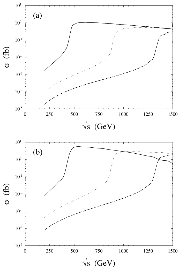
FIG. 2.: The cross section, $\sigma(e^{-}\gamma\to e^{+}\mu^{-}\mu^{-})$ as a function of $\sqrt{s_{ee}}$. In both cases the solid line is for $M_{\Delta}=400$ GeV, the dotted line for $M_{\Delta}=800$ GeV and the dashed line for $M_{\Delta}=1200$ GeV. (a) is for all three final state particles being detected and (b) is when only the $\mu^{-}\mu^{-}$ pairs are observed and the positron is lost down the beam pipe.

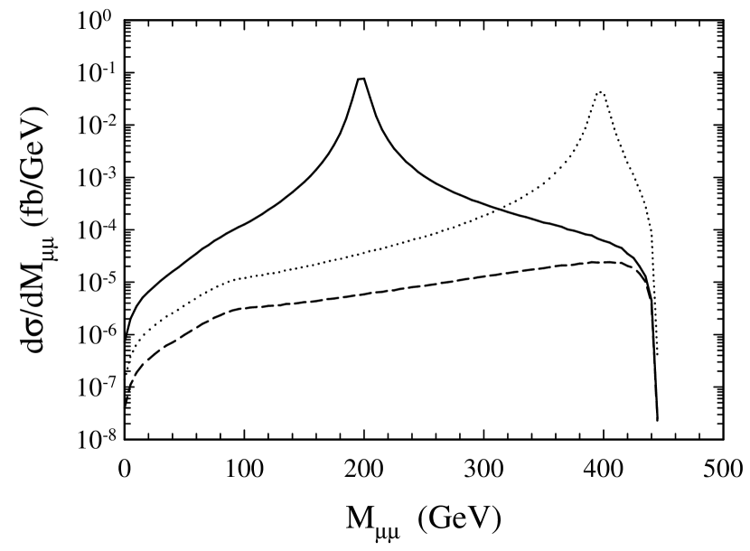
FIG. 3.: The invariant mass distribution of the final state like-sign muons in the process $e^{-}\gamma\to e^{+}\mu^{-}\mu^{-}$ for $\sqrt{s}=500$ GeV. The solid line is for $M_{\Delta}=400$ GeV, the dotted line for $M_{\Delta}=800$ GeV and the dashed line for $M_{\Delta}=1200$ GeV. All curves are for $\Gamma_{\Delta}=10+\Gamma_{f}$.

FIG. 4.: Discovery limits for doubly charged Higgs bosons as a function of the Yukawa coupling and $M_{\Delta}$ with $\sqrt{s}=500$ for different $\Gamma_{\Delta}=\Gamma_{b}+\Gamma_{f}$ scenarios. The dashed curve is for $\Gamma_{b}=0$, the dotted curve for $\Gamma_{b}=1.5$ GeV (the narrow width case), and the dot-dashed curve for $\Gamma_{b}=10$ GeV (the wide width case). The limits are based on observation of one event assuming an integrated luminosity of ${\cal L}=500$ fb^-1.

FIG. 5.: Discovery limits for doubly charged Higgs bosons as a function of the Yukawa coupling and $M_{\Delta}$ for different discovery probabilities. The dotted curves are based on 63% probability corresponding to 1 expected event, the dashed curves are based on 95% probability (3 events), and the long-dashed curves are based on 99% probability (4.6 events). The 3 curves on the left are for $\sqrt{s}=500$ GeV and those on the right are for $\sqrt{s}=1500$ GeV. In all cases an integrated luminosity of ${\cal L}=500$ fb^-1 is assumed.

FIG. 6.: Discovery limits for doubly charged Higgs bosons as a function of the Yukawa coupling and $M_{\Delta}$ for center of mass energies of $\sqrt{s}=500$, 800, 1000, and 1500 GeV, appropriate to the LC. The limits are based on 95% probability of discovery assuming an integrated luminosity of ${\cal L}=500$ fb^-1. (a) is for the case of all three final state particles being observed and (b) is the case of only the two final state muons being observed.

FIG. 7.: Discovery limits for doubly charged Higgs bosons as a function of the Yukawa coupling and $M_{\Delta}$ for center of mass energies of $\sqrt{s}=3$, 5, and 8 TeV, appropriate to CLIC. The limits are based on 95% probability of discovery assuming an integrated luminosity of ${\cal L}=500$ fb^-1. (a) is for the case of all three final state particles being observed and (b) is the case of only the two final state muons being observed.

TABLE I.: 95% probability mass discovery limits of doubly charged Higgs bosons, given in TeV, in $e\gamma$ collisions. Results are shown for $\sqrt{s}=500$, 800, 1000, 1500 GeV appropriate to the LC and $\sqrt{s}=3$, 5, and 8 TeV appropriate to CLIC. In all cases we assume an integrated luminosity of ${\cal L}=500$ fb^-1. The cases shown are for $e^{+}\mu^{-}\mu^{-}$ detected and for the $e^{+}$ lost down the beam for the narrow $\Delta$ case with the representative Yukawa coupling of $h=0.1$. Results for the broad $\Delta$ case are essentially the same.

$\sqrt{s}$	$e^{+}\mu^{-}\mu^{-}$ observed	$\mu^{-}\mu^{-}$ observed
(TeV)	$M_{\Delta}$ (TeV)	$M_{\Delta}$ (TeV)
0.5	0.54	0.71
0.8	0.78	0.98
1.0	0.95	1.15
1.5	1.38	1.57
3.0	2.72	2.83
5.0	4.51	4.58
8.0	7.21	7.30