Abstract

Nucleon form factors at high momentum transfer $t$ are treated in the framework of generalized parton distributions (GPD’s). The possibility of obtaining information about parton high transverse momentum components by application of GPD’s to form factors is discussed. This is illustrated by applying an ad-hoc 2-body parton wave function to elastic nucleon form factors $F_{1}$ and $F_{2}$, the $N\to\Delta$ transition magnetic form factor $G^{*}_{M}$, and wide angle Compton scattering (WACS) form factor $R_{1}$.

1 Introduction.

1.1 Valence PQCD.

One of the most studied questions relating to the properties of hadrons during the past decades has been how to describe exclusive reactions, and in particular electromagnetic form factors, in experimentally accessible regions of energy and momentum transfer. For momentum transfers of tens of GeV², corresponding to characteristic wavelengths of less than 0.1 fm, ordinary constituent quark or flux tube models, which are a mainstay at much lower momentum transfers, appear to be inadequate, especially with increasing momentum transfer. Improved fits have been possible through modification of CQM’s such as the introduction of quark form factors [1].

During the 1980’s there was considerable theoretical progress in the description of exclusive reactions at asymptotically high momentum transfers in terms of the fundamental current quarks, applying valence perturbative QCD (PQCD),  [2, 3, 4] together with SVZ [5] sum rules. Among the most important consequences of valence PQCD are the so called constituent counting rules, which predict relatively simple dependences of exclusive amplitudes as functions of momentum transfer. Many reactions experimentally appear to obey these constituent counting rules. Also, the magnetic nucleon elastic form factors and some resonant transition form factors could be roughly accounted for in magnitude through the application of the QCD sum rules [4, 6, 7, 8], leading to the possibility that valence PQCD would be applicable at kinematic conditions achieved at current or planned accelerator facilities. However, it had also been pointed out [9, 10] that the results of utilizing PQCD sum rules led to seemingly unrealistic valence quark longitudinal momentum fraction distributions $\phi(x)$. When utilized in the PQCD calculations, these $\phi(x)$’s led to inconsistent application of PQCD.

Another prediction of PQCD is hadron helicity conservation. Recent experiments [11, 12] at Jefferson Lab (JLab), which have measured helicity non-conserving amplitudes for elastic and resonance form factors, have shown that at momentum transfers approaching 6 GeV² the approach to PQCD is not manifest.

1.2 Generalized Parton Distributions.

The recent evolution of the theoretical formalism of generalized parton distributions [13, 14, 15] (GPD’s) has shown promise of providing a framework for describing exclusive reactions in terms of parton degrees of freedom without invoking the internal hard mechanisms of valence PQCD. The GPD description has been discussed primarily in the reactions involving deeply virtual Compton scattering and meson production, at as high $Q^{2}$ and small $t$ as possible. This is the kinematic region in which it has been shown that the reaction mechanism can be factorized into a hard perturbative, and soft non-perturbative part [15], the so-called handbag process illustrated in fig. 1.

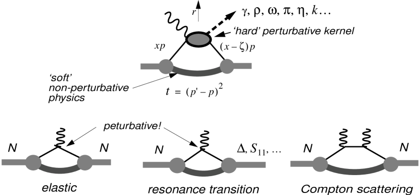
Figure 1: Diagrams representing the “handbag” mechanism; upper, deeply virtual Compton scattering and meson production; lower, nucleon elastic and resonance form factors, and wide angle Compton scattering.

The soft handbag is characterized by GPD’s which contain information about the distribution of quarks in the hadron. In particular, they give the amplitude that a quark with longitudinal momentum fraction $x$, in a hadron with momentum $p$, can be given a momentum kick $t=r^{2}$ with sideways component $r_{\perp}$, and re-absorbed by the hadron which emerges with a momentum $p-r$ (see fig. 1-top). Typically, hard electroproduction processes also require a longitudinal momentum transfer, characterized by a skewedness parameter $\zeta\equiv r_{\parallel}/p$. In the limit $t\to 0$ the certain GPD’s become identical with the deep inelastic scattering (DIS) structure functions, while others are not accessible in DIS.

A very important property of the GPD’s are sum rules which directly relate moments of the GPD’s to various hadronic form factors. For example, electron scattering form factors are the 0’th moments of the GPD’s.

For elastic scattering

$$F_{1}(t)=\int^{1}_{0}\sum_{q}\mathcal{F}^{q}_{\zeta}(x,t)dx$$ (1)

$$F_{2}(t)=\int^{1}_{0}\sum_{q}\mathcal{K}^{q}_{\zeta}(x,t)dx$$ (2)

where $q$ signifies both quark and anti-quark flavors. We work in a reference frame in which the total momentum transfer is transverse so that $\zeta$=0, and denote $\mathcal{F}^{q}(x,t)\equiv\mathcal{F}^{q}_{0}(x,t)$,  $\mathcal{K}^{q}(x,t)\equiv\mathcal{K}^{q}_{0}(x,t)$, etc.

For Compton scattering $\zeta=0$, and the appropriate form factor-like quantities [16] are the -1’th moments of the GPD’s

$$R_{1}(t)=\int^{1}_{0}\sum_{q}{1\over x}\mathcal{F}^{q}(x,t)dx$$ (3)

$$R_{2}(t)=\int^{1}_{0}\sum_{q}{1\over x}\mathcal{K}^{q}(x,t)dx$$ (4)

Resonance transition form factors access components of the GPD’s which are not accessed in elastic scattering or WACS. The $N\to\Delta$ form factors are related to isovector components of the GPD’s [17].

$$G^{*}_{M}=\int^{1}_{0}\sum_{q}\mathcal{F}^{q}_{M}(x,t)dx\ \ \ G^{*}_{E}=\int^{1}_{0}\sum_{q}\mathcal{F}^{q}_{E}(x,t)dx\ \ \ G^{*}_{C}=\int^{1}_{0}\sum_{q}\mathcal{F}^{q}_{C}(x,t)dx$$ (5)

where $G^{*}_{M}$, $G^{*}_{E}$ and $G^{*}_{C}$ are magnetic, electric and Coulomb transition form factors [18], and $\mathcal{F}^{q}_{M}$, $\mathcal{F}^{q}_{E}$, and $\mathcal{F}^{q}_{C}$ are axial (isovector) GPD’s, which can be related to elastic GPD’s in the large $N_{C}$ limit through isospin rotations. Similar relationships can be obtained for the $N\to S_{11}$ and other transitions.

The GPD’s as functions of $x$ give the contributions to the form factors due to quarks of flavor $q$ having momentum fraction $x$. As a function of $t$ they are directly related to the perpendicular momentum distribution of partons in the hadron wave function in ways which are inaccessible to DIS. The Fourier transforms of the GPD’s over $r_{\perp}$ give the transverse impact parameter distributions [19].

In particular, at high $|t|$ the resulting baryon form factors are strongly related to the high momentum components of the valence quark distribution amplitudes. This is illustrated in the following sections, in which a simple ad hoc power behavior of the high $k_{\perp}$ of the quark distribution is used.

2 Specific Examples.

2.1 Proton Dirac Form Factor ${\bf F_{1}}$.

The following is based on the development by Radyushkin [16], who calculated the proton helicity conserving form factor, $F_{1}$, assuming that the handbag can be expressed as an effectively two-body process, as illustrated in fig. 2. The proton wave function is factorized as follows

$$\Psi(x,k_{\perp})=\Phi(x)e^{-k^{2}_{\perp}/2x\bar{x}\lambda^{2}}$$ (6)

where $\bar{x}\equiv 1-x$, and $\lambda$ is a measure of the mean transverse momentum.

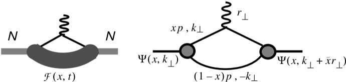
Figure 2: Schematic representation of the handbag mechanism as a two-body process.

In terms of the two-body wave functions eq. (6), the form factors are then expressed as:

$$F^{tb}=\int{\Psi^{*}(x,k_{\perp}+\bar{x}r_{\perp})\Psi(x,k_{\perp}){{d^{2}k_{\perp}}\over{16\pi^{3}}}}$$ (7)

Comparing eqs. (7) and (1) gives

$$\mathcal{F}(x,t)=\int_{0}^{1}dx\int{\Psi^{*}(x,k_{\perp}+\bar{x}r_{\perp})\Psi(x,k_{\perp}){{d^{2}k_{\perp}}\over{16\pi^{3}}}}$$ (8)

Insertion of eq. (6) into eq. (8), and evaluating the integral then gives

$$\mathcal{F}(x,t)={{x\bar{x}\lambda^{2}}\over{16\pi^{2}}}\Phi^{2}(x)e^{-\bar{x}t/4x\lambda^{2}}\equiv f(x)e^{-\bar{x}t/4x\lambda^{2}}$$ (9)

with valence quark distributions

$$f(x)=\sum_{q}e_{q}f^{v}_{q}(x)=e_{u}f^{v}_{u}(x)+e_{d}f^{v}_{d}(x).$$ (10)

The functions $f_{u}(x)$ and $f_{d}(x)$ are chosen to agree with the valence quark distributions $f^{v}_{q}(x)$ obtained directly in DIS. In particular, ref. [16] uses an empirical function found to agree with DIS

$$f^{v}_{u}(x)=1.89x^{-0.4}(1-x)^{3.5}(1+6x)$$ (11)

$$f^{v}_{d}(x)=0.54x^{-0.6}(1-x)^{4.2}(1+8x).$$ (12)

The function $\Phi(x)$ in eq. (13) is then written

$$\Phi_{q}^{2}(x)={{16\pi^{2}}\over{\lambda x\bar{x}}}f^{v}_{q}(x).$$ (13)

Substitution of eqs. (10) and  (13) into eq. (9), and then eq. (9) into eq. (1) yields for the proton Dirac form factor,

$$F_{1}(t)=\int^{1}_{0}\left[e_{u}f^{v}_{u}(x)+e_{d}f^{v}_{d}(x)\right]e^{-\bar{x}t/4x\lambda^{2}}dx$$ (14)

The only free parameter in the analysis is $\lambda$, which is a measure of the mean $k_{\perp}$. A good fit to SLAC data for $F_{1}$ up to $|t|\sim$ 8 GeV² was obtained. The resulting value of $\lambda^{2}\sim 0.7$ GeV² leads to a reasonable values of the mean square $k_{\perp}$ distributions: $\langle k_{\perp}^{2}\rangle\sim(270{\rm MeV)^{2}}$

2.2 Dirac Form Factor ${\bf F_{1}}$ at High ${\bf t}$

Data on $F_{1}$ exists [20] up to a $Q^{2}$  (= $-t$) of 32 GeV². Continuation of the calculated $F_{1}$ to higher $Q^{2}$ exhibits a steadily greater discrepancy with the data with increasing $Q^{2}$. This is shown in fig. 3.

Figure 3: Proton Dirac form factor $F_{1}$ as a function of $Q^{2}$. The data are from SLAC; circles ($\circ$) at lower $Q^{2}$ are from ref. [21], and pluses (+) at higher $Q^{2}$ are from ref. [20]. The dashed curve is the result of the soft wave function $\Psi_{soft}$. The solid curve is the result of adding a small hard component $\Psi_{hard}$

A subsequent  [22, 23] elaboration of the procedure of ref. [16] studied the relationship between model quark distribution amplitudes and form factors and Compton scattering. Ref.  [22] used a valence quark distribution which evolves to the asymptotic form [3, 24], $\Phi(x)\to\Phi^{as}(x)\propto 120x_{1}x_{2}x_{3}$. In addition to the valence $qqq$ configuration, higher Fock state contributions containing $qqq,g$ and $qqq,\bar{q}q$ were added. For the $k_{\perp}$ distribution, an exponential form similar to that in ref. [16] was used. For simplicity, the same $\lambda^{2}$ was used for all the three Fock state components, although the need to consider different $\lambda^{2}$’s for the valance and higher Fock states is discussed. It was found that the inclusion of the higher Fock states is significant, and can effect the form factors by as much as 20%. Overall the fit at higher $Q^{2}$  is improved, the fit at lower $Q^{2}$ somewhat deteriorated.

A Gaussian form of $\Psi$ cannot account simultaneously for the $F_{1}$ magnitude and shape over the entire range of $Q^{2}$. However,the addition of a small high $k_{\perp}$ component in eq. (6) can dramatically improve the fit. As an example, we choose a ad-hoc $1/k_{\perp}^{2}$ behavior with lower cutoff parameter $\Lambda$, and upper cutoff $k_{\perp,max}$:

$$\Psi(x,k_{\perp})=\Phi(x)\left(A_{s}e^{-k_{\perp}^{2}/2x\bar{x}\lambda^{2}}+A_{h}{{x\bar{x}\theta(k_{\perp}^{2}<k_{\perp,max}^{2})}\over{k_{\perp}^{2}+\Lambda^{2}}}\right)\equiv\Psi_{soft}+\Psi_{hard}$$ (15)

where $\lambda^{2}=0.7$ GeV² is fixed by the low to intermediate $Q^{2}$ behavior of $F_{1}$, $k_{\perp,max}=4$ GeV², and $\Lambda=0.35$ GeV². As seen in fig. 3, this small addition of $\Psi_{hard}$ in eq. (15) can account for the high, as well as the low $Q^{2}$ magnetic form factor. A value of $A_{h}/A_{s}$ = 0.065 was used in eq. (15) to obtain the solid curve. In all cases, the condition $\mathcal{F}(x,0)=f(x)$ is maintained. Also, note that $F_{1}(0)=\int\mathcal{F}(x,0)dx\approx 1$, which, is required in the definition of $F_{1}$. The function $\Psi(k_{\perp})=\int{\Psi(k_{\perp},x)dx}$ is shown in fig. 4.

The resulting GPDs as a function of $x$ for different values of $t$ are shown in fig. 5. It would be interesting to see how this transforms into the spacial impact distributions $f(x,b_{\perp})$ discussed in ref. [19].

Figure 4: The function $\Psi(k_{\perp})\equiv\int{\Psi(x,k_{\perp})dx}$ vs. $k_{\perp}$. The dashed curve is due to the soft Gaussian component $\Psi_{soft}$, with $\lambda^{2}=0.7\ {\rm GeV^{2}}$. The solid curve is $\Psi_{soft}+\Psi_{hard}$, with $A_{h}$ = 0.065, $k_{\perp,max}$ = 4 GeV, and cutoff parameter $\Lambda$ = 0.35 GeV.

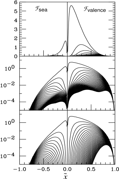
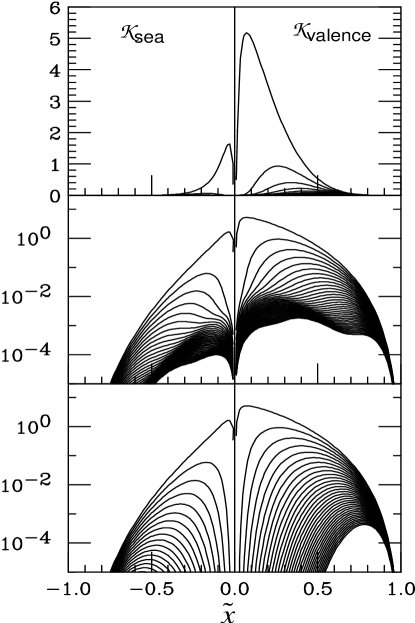
Figure 5: GPD’s as a function of $\tilde{x}$ for various values of $t$, where $\tilde{x}=x$ for valence quarks, and $\tilde{x}=-x$ for the sea quarks. The figures on the left and right are for $\mathcal{F}$ and $\mathcal{K}$ respectively. The graphs for positive $\tilde{x}$ represent the valence quark contribution, while the graphs for negative $\tilde{x}$ represent the sea quark contributions. The full GPDs are given by $\mathcal{F}=\mathcal{F}_{val}-\mathcal{F}_{sea}$ and $\mathcal{K}=\mathcal{K}_{val}-\mathcal{K}_{sea}$ respectively. The individual curves range from $|t|$ $\sim 0$ GeV² (highest curve in each panel) to $|t|$ = 35 GeV² (lowest curve in each panel). The upper and middle panels are the GPD’s for the full wave function $\Psi$ given in eq. (15), while those in the lowest panels are obtained using the soft wave function as in eq. (6). Note that the addition of the $\Psi_{hard}$ mainly affects the GPD’s at higher $|t|$ and $\tilde{x}<0.5$

Figure 6 shows the contribution to $F_{1}$ from different $k_{\perp}$ regions. It is clear that the high $Q^{2}$  regions of $F_{1}$ are selective of the high components of $\Psi(k_{\perp})$.

Figure 6: The contribution to $F_{1}$ from different regions in $\Psi(k_{\perp})$ of $k_{\perp}$. Each curve represents the contribution from regions of $k_{\perp}$ greater than the value indicated. The data are from SLAC; circles ($\circ$) at lower $Q^{2}$ are from ref. [21], and pluses (+) at higher $Q^{2}$ are from ref. [20].

2.3 Pauli form factor ${\bf F_{2}}$

Applying the analogous formalism as in ref. [16], Afanasev [25] modeled $\mathcal{K}(x,t)$ in eq. 2 as

$$\mathcal{K}^{q}(x,t)=k^{q}(x)e^{-\bar{x}t/4x\lambda^{2}}.$$ (16)

with $\lambda$ and the normalization at $Q^{2}$ = 0 free parameters.

Unlike the case for $f^{q}(x)$, an expression for $k^{q}(x)$ cannot be obtained from DIS. Reference [25] notes that asymptotically PQCD and the SVZ sum rules require an extra factor of $1-x$ for $k^{q}(x)$. In the present study, it is found that the simplest form $k^{q}(x)=(1-x)f^{q}(x)$ adequately describes the data. The expression for $F_{2}$ is then

$$F_{2}(t)=\int^{1}_{0}\left[e_{u}k^{v}_{u}(x)+e_{d}k^{v}_{d}(x)\right]e^{-\bar{x}t/4x\lambda^{2}}dx$$ (17)

Figure 7 shows $F_{2}$, and fig. 8 shows $Q^{2}F_{2}(Q^{2})/F_{2}(Q^{2})$ compared with the recent JLab data [12]. The obtained $G_{EP}/G_{MP}$, also compared with the recent JLab data is shown in fig. 9. For $F_{2}$ the best fit was obtained for $\lambda^{2}$ = 0.5, and $F_{2}(0)$ was normalized to $\kappa=1.79$. All other parameters, including $A_{H}$ and $\Lambda$ were fixed by $F_{1}$. The contribution of $\Psi_{soft}$ as in eq. (6) is also shown. The effects of inclusion of $\Psi_{hard}$ become important at around $Q^{2}$ = 8 GeV². The JLab upgrade includes measurements to about 15 GeV², which should test this.

Figure 7: Proton Pauli form factor $F_{2}$ as a function of $Q^{2}$. The dashed curve is the result of inclusion only of $\Psi_{soft}$ in eq. (15). The solid curve is the result of adding $\Psi_{hard}$

Figure 8: The ratio of the proton Dirac and Pauli form factors $Q^{2}F_{2}/F_{1}$ as a function of $Q^{2}$. The dashed curve is the result of including only $\Psi_{soft}$. The solid curve is the result of adding $\Psi_{hard}$. The data are the recent JLab results [12].

Figure 9: The ratio of the proton electric and magnetic form factors $G_{E}/G_{M}$ as a function of $Q^{2}$. The dashed curve is the result of inclusion only of $\Psi_{soft}$. The solid curve is the result of adding $\Psi_{hard}$. The data are the recent JLab results [12]

2.4 Wide angle Compton Scattering

The inclusion of $\Psi_{hard}$ in eq. (15) also directly affects wide angle Compton scattering (WACS). Analogous to the elastic electron scattering form factors $F_{1}$ and $F_{2}$ are the Compton “form factors” $R_{1}$ and $R_{2}$, which are related to the Klein-Nishina cross section:

$${{d\sigma}\over{dt}}=\left({{d\sigma}\over{dt}}\right)_{KN}R^{2}$$

with $R^{2}=R_{1}^{2}(t)+{{-t}\over{4m_{p}^{2}}}R_{2}^{2}(t)$. As in the case with electron scattering, $R_{2}(t)/R_{1}(t)$ is expected to fall as a power of $|t|$, so that the cross section at high $|t|$ is dominated by $R_{1}(t)$.

Since the integrals in $R_{1}$ and $R_{2}$ (eqs. (3, 4) are weighted with $1/x$, they may be expected to be more sensitive to the sea quark distribution. Reference [16] adds a sea quark contribution to $f_{Compton}$:

$$f_{Compton}=f_{Compton}^{val}+f_{Compton}^{sea}$$

with

$$f_{Compton}^{val}=e_{u}^{2}f^{v}_{u}(x)+e_{d}^{2}f^{v}_{d}(x)$$

and

$$f_{Compton}^{sea}=(e_{u}^{2}+e_{d}^{2}+e_{s}^{2})f^{sea}(x)$$

where $f^{v}_{u}$ and $f^{v}_{d}$ are parameterized as in eqs. (11) and ( 12), respectively, and $f^{sea}(x)$ is parameterized as follows:

$$f^{sea}(x)=0.5x^{-0.75}(1.0-x)^{7}$$

Figure 10 shows the result for $R_{1}(t)$ with and without the presence of $\Psi_{hard}$. All parameters in $\Psi_{soft}$ and $\Psi_{hard}$ are fixed by the fit to $F_{1}(Q^{2})$. The proposed experiments at JLab with a 12 GeV electron beam are expected to reach $|t|$ = 15 GeV², and therefore should be sensitive to the consistency of the approach. Figure 11 shows the contribution to $R_{1}$ from different $k_{\perp}$ regions of $\Psi(k_{\perp})$. It is clear that the high $|t|$ regions of $R_{1}$ are selective of the high components of $\Psi(k_{\perp})$.

Figure 10: The Compton form factor $R_{1}(t)$ vs. $t$, using $\Psi=\Psi_{soft}$ (dashed) and $\Psi=\Psi_{soft}+\Psi_{hard}$ (solid).

Figure 11: The contribution to $R_{1}$ from different regions in $\Psi(k_{\perp})$ of $k_{\perp}$. Each curve represents the contribution from regions of $k_{\perp}$ greater than the value indicated.

Reference [22] have also evaluated wide angle Compton scattering, and find the higher Fock components contribute an even more significant fraction of the form factors ($R_{1},R_{2}$) than in elastic scattering, especially at lower $|t|$, as may be expected.

2.5 $N\to\Delta$ transition.

The transition $N\to\Delta(1232)$ is purely isovector, which can be expressed in terms of three transition from factors [18]; magnetic $G_{M}^{*}(Q^{2})$, electric $G_{E}^{*}(Q^{2})$, and Coulomb (or scalar) $G_{C}^{*}(Q^{2})$, with $(p_{\Delta}-p)^{2}=t=-Q^{2}$. These can be expressed in terms of the isovector components of the GPD’s [17]:

$$G_{M}^{*}(t)=\int^{1}_{0}\sum_{q}\mathcal{F}_{M}^{(3)q}(x,t)dx$$

$$G_{E}^{*}(t)=\int^{1}_{0}\sum_{q}\mathcal{F}_{E}^{(3)q}(x,t)dx$$

$$G_{C}^{*}(t)=\int^{1}_{0}\sum_{q}\mathcal{F}_{C}^{(3)q}(x,t)dx$$

The experimental status of the $N\to\Delta$ transition magnetic form factor is shown in figure 12.

Figure 12: The $N\to\Delta$ magnetic form factor $G_{M}^{*}(Q^{2})$ relative to the dipole $G_{D}=3/(1+0.71Q^{2})^{2}$. The data points for $Q^{2}$ below 2.8 GeV² are from a compilation of ref. [26]. Those at $Q^{2}$ = 2.8 and 4.0 GeV² are recent JLab data [11]. The horizontal line reflects the $1/Q^{4}$ asymptotic PQCD shape, and the curve denoted GPD is discussed in the text.

The decrease in $G_{M}^{*}$ relative to $G_{D}$ indicates that the transition form factor is softer than that for elastic scattering. The soft part of the transition form factor can be modeled by assuming a different $\lambda$ parameter for $\Psi_{\Delta}$ than $\Psi_{P}$. Thus, we take

$$\Psi_{P,soft}(x,k_{\perp})=\Phi_{P}(x)e^{(-k^{2}_{\perp}/2x\bar{x}\lambda_{P}^{2})}$$

$$\Psi_{\Delta,soft}(x,k_{\perp})=\Phi_{\Delta}(x)e^{(-k^{2}_{\perp}/2x\bar{x}\lambda_{\Delta}^{2})}$$

For simplicity we have taken $\Phi_{\Delta}(x)=\Phi_{P}(x)=\Phi(x)$. This leads to

$$F_{N\Delta}(x,k_{\perp},t)={{x\bar{x}}\over{8\pi^{2}}}\left({{\lambda_{P}^{2}\lambda_{\Delta}^{2}}\over{\lambda_{P}^{2}+\lambda_{\Delta}^{2}}}\right)\Phi^{2}(x)e^{-{{\bar{x}|t|}\over{2x}}\left({{1}\over{\lambda_{P}^{2}+\lambda_{\Delta}^{2}}}\right).}$$

The curve passing through the data is obtained with $\lambda^{2}_{P\Delta}\equiv\lambda_{P}^{2}+\lambda_{\Delta}^{2}=0.38$ implying a transition $(k_{\perp})_{RMS}\sim(180)^{2}\ {\rm(MeV)^{2}}$, which is considerably smaller than the value obtained for elastic scattering from the proton. This also implies that the mean transition radius for the $N\to\Delta$ transition is also larger than for proton elastic scattering.

3 Conclusion.

The advent of the GPD formalism offers a framework to model the $k_{\perp}$ distributions of quarks which are involved in exclusive reactions. These distributions are constrained by providing simultaneous fits to several different reactions rather than by fitting form factors for a single specific reaction. Furthermore, specific reactions may be sensitive to specific components of GPD. For example the $N\to\Delta$ is selective of isovector components.

Within the two-body framework presented, high $Q^{2}$ (or$|t|$) form factors are sensitive to the high momentum components of the underlying wave functions. The sensitivities become significant at $Q^{2}$ or $|t|$ greater than about 7 or 8 GeV². Currently, only $G_{MP}$ experimental data extend to much higher values of $Q^{2}$. However, the proposed program of high $|t|$ exclusive measurements for the Jefferson Lab 12 GeV upgrade is anticipated to provide high quality data for all of the reactions discussed here.

The example given here for modeling the hard part of the wave function is purely ad-hoc and not meant as a rigorous theoretical procedure, but indicative of the sensitivity of high $|t|$ exclusive reactions to high momentum components of the nucleon parton distribution. More rigorous theoretical approaches are expected in parallel with the high quality data expected in the future.

Acknowledgements:

The author thanks Anatoly Radyushkin for much discussion and guidance. Richard Davidson is thanked for helpful discussions.

The work was partially supported by the National Science Foundation.

References

- [1] F. Cardarelli et al., Physics Letters B371, 7 (1996)
- [2] A.V. Efremov and A.V. Radyushkin, Theor. Math. Phys. 42, 97 (1980)
- [3] S. J. Brodsky and G. P. Lepage, Phys. Rev. D22, 2157 (1980).
- [4] V.L. Chernyak and I.R. Zhitnitsky, Physics Reports, 112, 173 (1984).
- [5] M.A. Shiffman, A.I. Vainstein and V.I.Zakharov, Nuc. Phys., B47,385,448,519 (1979).
- [6] C. E. Carlson and J. L. Poor, Phys. Rev. D38, 2758 (1988).
- [7] P. Stoler, Physics Reports226, 103 (1993).
- [8] G. Sterman and P. Stoler, Annual Reviews of Nuclear and Particle Science, 47, 193 (1997).
- [9] A. V. Radyushkin, Nucl. Phys. A527, 153c (1991).
- [10] N. Isgur and C. H. Lewellyn- Smith, Phys. Rev. Lett. 52, 1080 (1984);
- [11] V. V. Frolov, PhD thesis, Rensselaer Polytechnic Institute; V. V. Frolov, et al. Phys. Rev. Lett. 82,45 (1999).
- [12] M.K. Jones et al. Phys. Rev. Lett. 84,1398 (2000).
- [13] X. Ji, Phys. Rev. Lett. 78, 610 (1997);
- [14] A. Radyushkin, Phys. Lett. B380,417 (1996); Phys. Rev. D56,5524 (1997).
- [15] J. Collins, L. Frankfort, and M. Strikman, Phys. Rev., D56, 2982 (1997).
- [16] A. Radyushkin, Phys. Rev. D58,114008 (1998).
- [17] K.Goeke, M.V. Polyakov, and M. Vanderhaeghen, Prepriint hep-ph/01060112, 1 June, (2001)
- [18] H.F. Jones and M.D. Scadron, Annals of Physics 81, 1 (1979).
- [19] Phys. Rev. D62,0701503 (2000); hep-ph/0005108.
- [20] R.G. Arnold et al., Phys. Rev. Lett. 57, 174 (1986).
- [21] L. Andihavis et al., Phys. Rev. D50, 5491 (1994).
- [22] M.Diehl, Th. Feldmann, R. Jakob and P. Kroll, Eur. Phys. C8, 409 (1999); hep-ph/9811253.
- [23] M.Diehl, Th. Feldmann, R. Jakob and P. Kroll, Nucl. Phys. B596, 33 (2001), Erratum-ibid. B605, 647 (2001); hep-ph/0009255.
- [24] J. Bolz and P. Kroll, Z. Phys. A356,327 (1996).
- [25] A. Afanasev, E-print: hep-ph/9910565; “Proceeding of the JLAB-INT Workshop on Exclusive and Semi-Exclusive Processes at High Momentum Transfer”, C. Carson and A. Radyushkin, eds. World Scientific (2000). May 1999
- [26] S.S. Kamalov and S. N. Yang, Phys. Rev. Lett. 83, 4494 (1999).