August 2001 HIP-2001-45/TH

TIFR/TH/01-34

Vacuum stability bounds in Anomaly and Gaugino Mediated SUSY breaking models

Emidio Gabrielli^a,, Katri Huitu^a,, Sourov Roy^b,

^aHelsinki Institute of Physics,
POB 64,00014 University of Helsinki, Finland
^bDepartment of Theoretical Physics
Tata Institute of Fundamental Research
Homi Bhabha Road, Mumbai - 400 005, India

We constrain the parameter space of the minimal and gaugino–assisted anomaly mediation, and gaugino mediation models by requiring that the electroweak vacuum corresponds to the deepest minimum of the scalar potential. In the framework of anomaly mediation models we find strong lower bounds on slepton and squark masses. In the gaugino mediation models the mass spectrum is forced to be at the TeV scale. We find extensive regions of the parameter space which are ruled out, even at low $\tan{\beta}$. The implications of these results on the g-2 of the muon are also analyzed.

Supersymmetry (SUSY) is considered to be one of the most probable alternatives for the physics beyond the Standard Model. The most general version of the minimal supersymmetric standard model includes a large number of parameters with which the ignorance of the supersymmetry breaking is parametrized. Unfortunately with all the parameters, the model becomes untraceable, and consequently several ways to simplify the parameter space have been considered. These simplifications are based on the fact that if it were known how supersymmetry is broken, one could calculate the soft supersymmetry breaking parameters. There are a large number of supersymmetry breaking scenarios, which give acceptable phenomenology at least for some part of the parameter space.

In recent years the branes, which are typical in models with extra dimensions, have been found to fit naturally with the idea of breaking supersymmetry in a hidden sector. Inspired by extra dimensions, anomaly mediated (AMSB) [1] and gaugino mediated ($\tilde{g}$MSB ) [2] supersymmetry breaking have been constructed. Here we will assume two parallel branes, which are located in one extra dimension, as proposed by Randall and Sundrum [1]. One of the branes contains the hidden sector, while the other brane contains the ordinary matter. Gravity is in the bulk. Since there are no tree-level couplings between the fields in the observable and hidden sectors, the anomaly mediated contribution may be the dominant one. In the pure AMSB scenario the slepton masses have negative squares, but there are several proposals to fix the scenario [3]. The most straightforward way would be to add a constant term to the scalar masses (minimal anomaly mediation, mAMSB ). With extra dimensions assuming gauge multiplets in the higher dimensional bulk, it was found in [4] that at one loop the squared slepton masses obtain contributions, which would be of the correct size for solving the slepton mass problem (gaugino assisted anomaly mediation, $\tilde{g}$AMSB ). Also in the gaugino mediation models, the gauge superfields propagate in the bulk in addition to gravity, but in the $\tilde{g}$MSB models they couple at tree-level to a singlet at the SUSY breaking brane. The gaugino becomes massive, if the vacuum expectation value (VEV) of the singlet is nonvanishing, thus breaking supersymmetry.

Since none of the ways to break supersymmetry is compelling, it is essential to study all the ways to restrict the parameter space of the different models. In addition to experimental bounds, there are theoretical requirements, which must be fulfilled. In this letter we will study the unbounded directions of the vacua of the SUSY breaking models described above.

The presence of a large number of charged and colored scalar fields can generate dangerous minima in the scalar effective potential ($V$) of MSSM giving rise to an unacceptable color and electric charge breaking [5]. In the analysis of vacuum stability bounds, radiative corrections to $V$ play an important role. They are necessary in order to stabilize $V$ under variations of the renormalization scale, since the exact expression for the renormalized effective potential should not depend upon this scale. Due to this property, the search for these minima can be strongly simplified by choosing an appropriate scale ($\hat{Q}$) for which the one-loop corrections are minimized. A useful approximation consists of analyzing the minima of the tree-level potential ($V_{tree}$) evaluated at this scale $\hat{Q}$ and then requiring that the dangerous minima are never deeper than the real minimum.

A complete study of vacuum stability bounds in MSSM has been recently carried out in [5]. In this work, two classes of necessary and sufficient conditions have been found. The strongest ones come from avoiding directions in the field space along which $V_{tree}$ (calculated at $\hat{Q}$ scale) becomes unbounded from below (UFB). These are given by a set of three conditions, namely UFB-1,2,3. The other class of constraints follow from avoiding the charge and color breaking (CCB) minima deeper than the realistic minimum. However, even though these conditions have been obtained in a model independent way, the phenomenological analysis has been carried out in specific models [5, 6].

In a more recent paper [8], the vacuum stability bounds have been analyzed for the mAMSB models. In this work it was found that UFB constraints (UFBc) would set quite strong bounds on sparticle spectra. In particular, selectron mass below $380$ GeV and stau mass below $270$ GeV can be ruled out by applying the present experimental bounds on sparticle masses, especially the lower bound on chargino mass from LEP2 [9]. Since the only difference in the parameter space between the $\tilde{g}$AMSB and the mAMSB model lies in the nonuniversality of the extra contribution to the scalar masses, one should expect that also for $\tilde{g}$AMSB models one gets strong bounds. The major difference in the models comes from the weighted sum over the quadratic Casimir for the matter scalar representations, leading to nonuniversal contributions, whose relative strengths are given by [4]

$$v=(Q,u,d,L,e,H_{2},H_{1})=(\frac{21}{10},\frac{8}{5},\frac{7}{5},\frac{9}{10},\frac{3}{5},\frac{9}{10},\frac{9}{10}).$$ (1)

If there is a tree-level coupling of gauge fields to the SUSY breaking brane, with a singlet which receives a VEV, the gauginos get a SUSY breaking mass [2]. Minimally the $\tilde{g}$MSB model has three parameters, namely the Higgs mixing parameter $\mu$, the common gaugino mass $M_{1/2}$ and the compactification scale $M_{c}$. Following Schmaltz and Skiba in [2], we assume that at the compactification scale the soft breaking $A$ parameters, as well as the soft scalar masses, vanish and $M_{c}$ is in the range $M_{GUT}\ \hbox to0.0pt{\raise 2.0pt\hbox{$<$}\hss}{\lower 2.0pt\hbox{$\sim$}}\ M_{c}\ \hbox to0.0pt{\raise 2.0pt\hbox{$<$}\hss}{\lower 2.0pt\hbox{$\sim$}}\ M_{Planck}/10$. However, since we are interested in analyzing a more general scenario than in [2], we will take $\tan{\beta}$ as a free parameter. This is effected by relaxing the condition of vanishing soft $B$ parameter at $M_{c}$ scale assumed in [2].

Before presenting our results, we briefly recall the definition of the strongest UFB condition, namely UFB-3 in the notation of reference [5]. This is obtained by avoiding dangerous UFB directions along the down type Higgs VEV $\langle H_{1}\rangle=0$, after suitable choices for down–squarks and slepton VEVs have been taken in order to cancel (or keep under control) the $SU(3)$, $SU(2)_{L}$, and $U(1)_{Y}$ D-terms. For any value of $H_{2}$, such that $|H_{2}|<M_{X}$ (where $M_{X}$ is the high scale where soft breaking terms are generated), and

$$|H_{2}|>\sqrt{\frac{\mu^{2}}{4\lambda_{e_{j}}}+\frac{4m_{L_{i}}^{2}}{g_{Y}^{2}+g_{2}^{2}}}-\frac{|\mu|}{2\lambda_{e_{j}}}$$ (2)

the following UFB-3 (strongest) condition must be satisfied

$$V_{UFB-3}(Q=\hat{Q})>V_{{\rm min}}(Q=M_{S})$$ (3)

where

$$V_{UFB-3}=\left(m_{H_{2}}^{2}+m_{L_{i}}^{2}\right)|H_{2}|^{2}+\frac{|\mu|}{\lambda_{e_{j}}}\left(m_{L_{j}}^{2}+m_{e_{j}}^{2}+m_{L_{i}}^{2}\right)|H_{2}|-\frac{2m_{L_{i}}^{4}}{\left(g_{Y}^{2}+g_{2}^{2}\right)}$$ (4)

with $i\neq j$, where $\lambda_{e_{i}}$ are the Yukawa couplings of the leptons $e_{i}$. In Eq.(4), the $\mu$ term is the usual bilinear coupling between the Higgs doublets $H_{1,2}$ in the superpotential, and $m^{2}_{H_{1,2}}$, $m^{2}_{L_{i}}$, and $m^{2}_{e_{j}}$ are the soft–breaking terms for the Higgs doublets, left–, and right–handed sleptons, respectively (with $i,j=1,2,3$ generation indices). Finally, $g_{Y}$ and $g_{2}$ correspond to the hypercharge and weak gauge couplings respectively. If Eq.(2) is not satisfied, then the expression for $V_{UFB-3}$ is the following

$$V_{UFB-3}=m_{H_{2}}^{2}|H_{2}|^{2}+\frac{|\mu|}{\lambda_{e_{j}}}\left(m_{L_{j}}^{2}+m_{e_{j}}^{2}\right)|H_{2}|+\frac{1}{8}\left(g_{Y}^{2}+g_{2}^{2}\right)\left(|H_{2}|^{2}+\frac{|\mu|}{\lambda_{e_{j}}}|H_{2}|\right)^{2}$$ (5)

It is clear that the optimum choice for the more restrictive condition is obtained by the replacement of $\lambda_{e_{j}}$ with the Yukawa coupling of the tau ($\lambda_{e_{j}}\rightarrow\lambda_{e_{3}}$) in Eqs.(2,4,5). In Eq.(3) $V_{{\rm min}}(\hat{Q}=M_{S})$ is the value of the tree-level (neutral) scalar potential calculated at the realistic minimum

$$V_{{\rm min}}=-\frac{1}{2\left(g_{Y}^{2}+g_{2}^{2}\right)}\left(\sqrt{\left(m_{H_{1}}^{2}+m_{H_{2}}^{2}+2\mu^{2}\right)^{2}-4|m_{3}|^{4}}-m_{H_{1}}^{2}+m_{H_{2}}^{2}\right)^{2}$$ (6)

and at the scale $M_{S}\simeq\sqrt{m_{\tilde{t}_{L}}m_{\tilde{t}_{R}}}$. The appropriate scale $\hat{Q}$ where $V_{UFB-3}$ should be evaluated (in order to minimize the one-loop corrections) is given by [5]

$$\hat{Q}\simeq Max(g_{2}|e|,\lambda_{top}|H_{2}|,g_{2}|H_{2}|,g_{2}|L_{i}|,M_{S})$$ (7)

where

$$|L_{i}|^{2}=-\frac{4m_{L_{i}}^{2}}{g_{Y}^{2}+g_{2}^{2}}+\left(|H_{2}|^{2}+|e|^{2}\right)~{}~{},~{}~{}|e|=\sqrt{\frac{|\mu|}{\lambda_{e_{i}}}|H_{2}|}\,.$$ (8)

In Figs. (1a,b)–(2a,b) and (3a,b) we show our results for the anomaly and gaugino mediation models respectively. In the first class of models, in addition to $\tan{\beta}\equiv\frac{<H_{2}>}{<H_{1}>}$ and the $\mu$ term, there are two more free parameters, the gravitino mass $m_{3/2}$ and $m_{0}$, which sets the mass scale for the extra contribution $\Delta m^{2}(i)$ to the scalar masses (with $i=H_{1,2},Q,u,d,L,e$). In the mAMSB model $\Delta m^{2}(i)$ is taken universal for all the scalars, namely $\Delta m^{2}(i)=m_{0}^{2}$. The $\mu$ term, as usual, is fixed by requiring the correct electroweak breaking condition, while the sign of $\mu$ ($sign(\mu)$) remains a free parameter in both models.

Our results correspond to $sign(\mu)$ for which the SUSY contribution to the anomalous magnetic moment of the muon (g–2)_μ is always positive. This choice is motivated by the recent measurement of (g–2)_μ at BNL, where a $2.6\sigma$ deviation from the SM prediction has been reported [10]. In particular, this deviation favors large and positive SUSY contributions to (g–2)_μ which are achieved by large $\tan{\beta}$ values. However, while the UFB-3 condition in Eq.(3) does not depend on $sign(\mu)$, this sign affects the physical spectrum for chargino, sleptons, and squarks and so their corresponding UFB bounds.

In Fig.(1a) we show our results, in the $(m_{3/2},m_{0})$ plane, for the allowed and disallowed regions by UFBc. In addition, the regions ruled out by experimental lower bounds on chargino and stau masses, respectively $m_{\chi}<86$ GeV and $m_{\tilde{\tau}}<82$ GeV [9], are also indicated. Continuous and dashed curves correspond respectively to $\tan{\beta}=5$ and $40$. Since SUSY contributions to (g–2)_μ and $b\to s\gamma$ are enhanced by $\tan{\beta}$, we show them only for $\tan{\beta}=40$. In particular, green and red shaded regions indicate, respectively, the allowed area of BNL deviation on (g–2)_μ at 2.6 $\sigma$ level and the excluded one by $b\to s\gamma$ at 90% of C.L.. In Fig.(1b) we show the UFB allowed and disallowed areas in the $(m_{\chi},m_{\tilde{\tau}})$ and $(m_{\chi},m_{\tilde{t}})$ planes, where $m_{\tilde{t}}$ indicate the mass of the lightest stop.

From these results we see that UFBc can set quite strong bounds on the relevant parameter space of the mAMSB model. For instance, the disallowed regions coming from the lower bound on stau mass are well inside the UFB disallowed area. The combined effect of the UFBc and the experimental lower bound on chargino mass, set a lower bound on $m_{0}$ of the order of 400 GeV and slightly depending on $\tan{\beta}$. Moreover, from the results in Fig.(1b) and for $\tan{\beta}=5~{}(40)$, they can set lower bounds of the order of 400 (300) GeV and 550 (530) GeV for the stau and stop masses respectively. For the opposite $sign(\mu)$ we get respectively 360 (300) GeV and 470 (510) GeV. Our results are in agreement with the corresponding ones in reference [8].

These results can be roughly understood as follows. The UFB-3 condition in Eq.(3) might become very strong due to the presence of the first term proportional to $m_{H_{2}}^{2}|H_{2}|^{2}$ in Eqs.(4) and (5). This term is negative (due to the fact that $m_{H_{2}}^{2}$ has to ensure the correct electroweak symmetry breaking), leaving $V_{\rm UFB-3}$ very deep for large values of $|H_{2}|$. However, the larger are the scalar masses (obtained by increasing $m_{0}$) the larger is the term $m_{L_{i}}^{2}|H_{2}|^{2}$ and the other ones proportional to $|H_{2}|$, leaving UFB-3 weaker. The main dependence of UFB-3 bounds with $\tan{\beta}$ is due to the second term in Eqs.(4)–(5) which is proportional to the inverse of the Yukawa coupling of the tau ($\lambda_{e_{3}}$). By taking into account that the coefficient of $\lambda^{-1}_{e_{3}}$ is always positive and $\lambda^{-1}_{e_{3}}$ decreases with $\tan{\beta}$, the larger is $\tan{\beta}$, the smaller the second term becomes, and thus makes UFB-3 stronger. However, from Fig.(1b) we see that the behavior of UFBc with $\tan{\beta}$ is reversed in $(m_{\chi},m_{\tilde{\tau}})$ plane, while in the $(m_{\chi},m_{\tilde{t}})$ one it is almost independent on $\tan{\beta}$. This is due to the fact that the stau mass is more sensitive to $\tan{\beta}$ than the stop one.

In Fig.(2a,b) we show the same results as in Fig.(1a,b), but for the $\tilde{g}$AMSB model. The $m_{0}$ parameter is defined here as $\Delta m^{2}(L)\equiv m_{0}^{2}$, where $(L)$ is the slepton doublet, while the other contributions to the scalar masses $\Delta m^{2}(i)$ are predicted in terms of the ratio of weight Casimirs in Eq.(1). Note that the above considerations about the UFB-3 constraint hold for this model as well. From the results in Fig.(1a,b) we see that the $\tilde{g}$AMSB model is slightly disfavored by UFBc, when compared to the mAMSB one. The main reason is that in $\tilde{g}$AMSB model the terms $\Delta m^{2}(i=Q,u,d)$ for squarks are larger than $\Delta m^{2}(i=L,e)$ for sleptons, due to larger Casimir factors in Eq.(1). Indeed, as shown in [5, 6], models with small slepton masses and large squark masses are disfavored by UFB-3. This is because the larger is the stop mass, the more negative is $m_{H_{2}}^{2}$, due to larger renormalization group contribution. Smaller $m_{L_{i}}^{2},~{}m_{e_{j}}^{2}$, make the $V_{UFB-3}$ more negative, and thus the UFB-3 bound becomes stronger. Finally, combining in Fig.(2b) experimental bounds on chargino mass with UFBc, we obtain, for $\tan{\beta}=5~{}(40)$, lower bounds of the order of 450 (360) GeV and 670 (690) GeV for stau and stop masses respectively. For the opposite $sign(\mu)$ we get respectively 430 (360) GeV and 620 (680) GeV.

In Fig.(3a) and (3b) we present the results for the $\tilde{g}$MSB model, with $SU(5)$ and $SO(10)$ unified groups respectively. Here the free parameters, in addition to $\mu$ and $\tan{\beta}$, are the gaugino mass $M_{1/2}$ at GUT scale and $t_{c}=\log(M_{c}/M_{GUT})$. Thus, the allowed range of $t_{c}$ is $0<t_{c}<4$. Since in this model the scalar masses ($\tilde{m}$) and trilinear couplings ($A$) are radiatively generated through the renormalization group running from the compactification scale down to the GUT scale, they will be proportional respectively to $\tilde{m}^{2}\propto M_{1/2}^{2}~{}\alpha_{GUT}~{}t_{c}$, and $A\propto M_{1/2}~{}\alpha_{GUT}~{}t_{c}$ times averaged Casimir factors, where $\alpha_{GUT}$ is the gauge coupling at GUT scale. For the exact expressions we have used the results of Ref. [2]. In Fig.(3a,b) we show the allowed and disallowed regions in the $(M,t_{c})$ plane, with $M=M_{1/2},~{}m_{\tilde{\tau}}$. In particular, regions below the continuous and dashed curves, corresponding to $\tan{\beta}=5$ and 20 respectively, are excluded. We stress that the corresponding plots for $M=m_{\chi}$ and $M=m_{\tilde{t}}$ almost overlap the $M=M_{1/2}$ and $m_{\tilde{\tau}}$ curves respectively. From these results we see that the SUSY spectrum is above 1 TeV for most of the parameter space, even for $\tan{\beta}=5$. Besides, for $\tan{\beta}>20$, the allowed regions are above the dashed lines, leading to much stronger bounds. These results can be understood by noting that scalar masses are proportional to gaugino mass $M_{1/2}$, being induced by radiative corrections, and are enhanced by $t_{c}$ which parametrizes the size of corrections from extra dimensions. As explained above, increasing $M_{1/2}$ (and $t_{c}$) increases the scalar masses, relaxing the UFB-3 constraint. Note that at $\tan{\beta}=20$, regions below $t_{c}\ \hbox to0.0pt{\raise 2.0pt\hbox{$<$}\hss}{\lower 2.0pt\hbox{$\sim$}}\ 2.6$ and $t_{c}\ \hbox to0.0pt{\raise 2.0pt\hbox{$<$}\hss}{\lower 2.0pt\hbox{$\sim$}}\ 1.5$ are excluded by UFBc for $SU(5)$ and $SO(10)$ respectively. Roughly the same results apply for the opposite $sign(\mu)$.

Now we discuss the impact of UFBc on the (g–2)_μ of the muon. Recently the predictions for (g–2)_μ in the framework of anomaly mediation and gaugino mediation models have been analyzed in Ref. [11]. However, in this work, UFBc were not taken into account. From the results in Figs.(1a),(2a) we see that in both anomaly mediation models these constraints strongly affect (g–2)_μ , leaving this class of models disfavored for explaining the BNL deviation (at $2\sigma$ level), especially $\tilde{g}$AMSB . However, in the framework of $\tilde{g}$MSB models, the effect of UFBc on (g–2)_μ is very strong. As shown in Figs.(3a,b), the (g–2)_μ allowed regions are completely ruled out by UFBc.

Summary. We have analyzed restrictions from UFB constraints on AMSB and $\tilde{g}$MSB models, which are closely connected to the ideas of extra dimensions. Our results show that the experimental limits on chargino mass puts strong bounds on slepton and squark masses in AMSB models, and the whole mass spectrum is very high for $\tilde{g}$MSB models, leading to problems with naturalness requirement for most of the parameter space. If the experimental deviation in (g–2)_μ is due to supersymmetry, only small windows in the parameter space of the AMSB models remain open, and the $\tilde{g}$MSB models are ruled out.

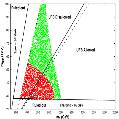
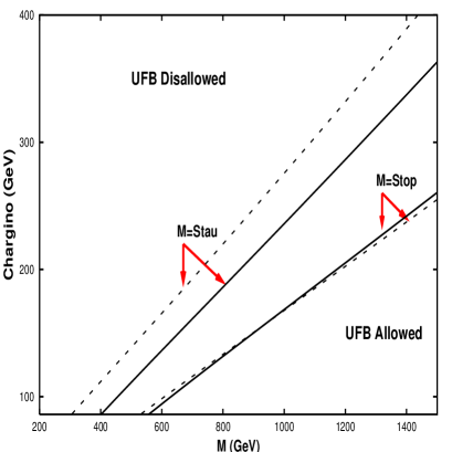
Figure 1: On the left (a), the allowed region by UFB-constraints in ($m_{0},m_{3/2}$) plane is shown in the mAMSB model. Solid and dashed lines corresponds to $\tan\beta=5$ and 40 respectively. For $\tan\beta$=40 we have also indicated the area forbidden by $b\rightarrow s\gamma$ results (red shaded area) and allowed by the (g–2)_μ results (green shaded area). Other than UFB, lines come from experimental lower limits as indicated in the plot. On the right (b), the allowed ranges for $\tilde{\tau}$ and $\tilde{t}$ masses are shown in ($m_{\chi},M$) plane. Solid and dashed lines as before.

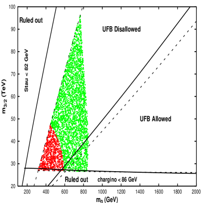
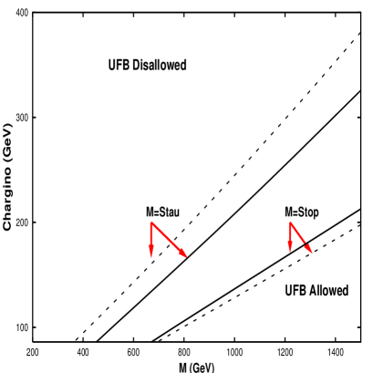
Figure 2: As Figure 1 but for $\tilde{g}$AMSB model.

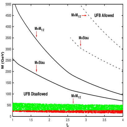
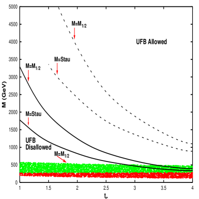
Figure 3: The allowed UFB ranges for the stau $(M=m_{\tilde{\tau}})$ and gaugino $(M=M_{1/2})$ masses are shown in ($M,t_{c}$) plane for the $\tilde{g}$MSB model with $SU(5)$ (left (a)) and $SO(10)$ (right (b)) unified groups. Solid and dashed lines correspond to $\tan\beta=5$ and 20 respectively. Red and green shaded areas as in Fig.(1), but for $\tan{\beta}=20$. Regions below red shaded areas are excluded by $m_{\tilde{\tau}}<82$ GeV.

Acknowledgements

This work was partially supported by the Academy of Finland (project nos. 48787 and 163394). S.R. wishes to acknowledge the hospitality provided by the Helsinki Institute of Physics, where a part of this work was done.

References

- [1] L. Randall, R. Sundrum, B557, 79 (1999); G.F. Giudice, M.A. Luty, H. Murayama, R. Rattazzi, JHEP 9812, 027 (1998) ; J.A. Bagger, T. Moroi, E. Poppitz, JHEP 0004, 009 (2000).
- [2] D.E. Kaplan, G.D. Kribs, M. Schmaltz, Phys. Rev. D62, 035010 (2000); Z. Chacko, M.A. Luty, A.E. Nelson, E. Ponton, JHEP 0001, 003 (2000); M. Schmaltz, W. Skiba, Phys.Rev. D62, 095005 (2000).
- [3] A. Pomarol, R. Rattazzi, JHEP 9905, 013 (1999); R. Rattazzi, A. Strumia, J.D. Wells, B576, 3 (2000); Z. Chacko, M. Luty, E. Pontón, Y. Shadmi, Y. Shirman, hep-ph/0006047; E. Katz, Y. Shadmi, Y. Shirman, JHEP 9908, 015 (1999); Z. Chacko, M.A. Luty, I. Maksymsk, E. Pontón, JHEP 0004, 001 (2000); I. Jack, D.R.T. Jones, B482, 167 (2000); M. Carena, K. Huitu, T. Kobayashi, B592, 164 (2001).
- [4] D.E. Kaplan, G.D. Kribs, JHEP 0009, 048 (2000).
- [5] J.A. Casas, A. Lleyda, C. Muñoz, Nucl. Phys. B471, 3 (1996).
- [6] A. Datta, A. Kundu, A. Samanta, Phys. Rev. D63, 015008 (2001); S.A. Abel, B.C. Allanach, JHEP 0007, 037 (2000); J.A. Casas, A. Ibarra, C. Muñoz, Nucl. Phys. B554, 67 (1999); S. Abel, T. Falk, Phys.Lett. B444, 427 (1998); J.A. Casas, S. Dimopoulos, Phys.Lett. B387, 107 (1996); H. Baer, M. Brhlik, D. Castano, Phys.Rev. D54, 6944 (1996); J.A. Casas, A. Lleyda, C. Muñoz, Phys. Lett. B380, 59-67 (1996), Phys. Lett. B389, 305 (1996).
- [7] A. Riotto, E. Roulet, Phys.Lett. B377, 60 (1996); A. Kusenko, P. Langacker, G. Segre, Phys.Rev. D54, 5824 (1996).
- [8] A. Datta, A. Kundu, A. Samanta, hep-ph/0101034.
- [9] M. Elsing (DELPHI Collaboration) presentations on Feb. 27, 2001, available from http://www.cern.ch/~offline/physics_links/lepc.html.
- [10] H.N. Brown et al. (Muon () Collaboration), Phys.Rev.Lett. 86, (2001) 2227; A. Czarnecki, W.J. Marciano, Phys. Rev. D64, (2001) 013014, and references therein.
- [11] K. Enqvist, E. Gabrielli, K. Huitu, Phys. Lett. B512 (2001) 107.