KA-TP-20-2001 hep-ph/0108245

Yukawa coupling quantum corrections to the self couplings
of the lightest MSSM Higgs boson

Wolfgang Hollik and Siannah Peñaranda 

Institut für Theoretische Physik, Universität Karlsruhe
Kaiserstraße 12, D–76128 Karlsruhe, Germany

Abstract

A detailed analysis of the top-quark/squark quantum corrections to the lightest CP-even Higgs boson $(h^{0})$ self-couplings is presented in the MSSM. By considering the leading one-loop Yukawa-coupling contributions of ${\cal O}(m_{t}^{4})$, we discuss the decoupling behaviour of these corrections when the top-squarks are heavy compared to the electroweak scale. As shown analytically and numerically, the large corrections can almost completely be absorbed into the $h^{0}$-boson mass. Our conclusion is that the $h^{0}$ self-couplings remain similar to the coupling of the ${\rm SM}$ Higgs boson for a heavy top-squark sector.

1 Introduction

The Standard Model (${\rm SM}$) with minimal Higgs-field content could turn out not to be basic theoretical framework for describing electroweak symmetry breaking. In recent years supersymmetry (${\rm SUSY}$) has become one of the most promising theoretical ideas beyond the SM. The Minimal Supersymmetric Standard Model (${\rm MSSM}$) [1] is the simplest supersymmetric extension of the ${\rm SM}$ and at least as successful as the SM to describe the experimental data [2].

The Higgs sector of the MSSM [3] involves two scalar doublets, $H_{1}$ and $H_{2}$, in order to give masses to up- and down-type fermions in a way consistent with supersymmetry. After spontaneous symmetry breaking, induced through the neutral components of $H_{1}$ and $H_{2}$ with vacuum expectation values $v_{1}$ and $v_{2}$, respectively, the ${\rm MSSM}$ Higgs sector contains five physical states: two neutral CP-even scalars ($h^{0}$ and $H^{0}$), one CP-odd pseudoscalar ($A^{0}$), and two charged-Higgs states ($H^{\pm}$). The Higgs potential of the ${\rm MSSM}$ is constrained by SUSY [3]: all quartic coupling constants are related to the electroweak gauge coupling constants, thus imposing various restrictions on the tree-level Higgs-boson masses, couplings and mixing angles. In particular, all tree-level Higgs parameters can be determined in terms of the mass of the CP-odd Higgs boson, $M_{A^{0}}$, and the ratio $\tan\beta={v_{2}}/{v_{1}}$. The other masses and the mixing angle $\alpha$ are then fixed, and the trilinear and quartic self-couplings of the physical Higgs particles can be predicted. The knowledge of the Higgs-boson self-couplings will be essential for establishing the Higgs potential and thus the Higgs mechanism as the basic mechanism for generating the masses of the fundamental particles [4].

The tree-level relations among the Higgs-boson masses in the MSSM acquire relevant radiative corrections, dominated by top-quark/squark loops [5]. Extensive effort has been devoted to progressive refinements of the radiative corrections for the Higgs-boson masses, with special emphasis on the prediction of the lightest MSSM Higgs-boson mass $M_{h^{0}}$, by using different techniques: renormalization group equations [6, 7], diagrammatic computations [8, 9, 10, 11], and a combination of both [12]. Besides the mass spectrum, the loop corrections influence the production cross sections and decay branching ratios [13].

Moreover, large quark/squark-loop corrections affect also the self-couplings of the neutral Higgs particles [14, 15, 16, 17, 18]. The loop contributions modify the mixing angle $\alpha$ for the neutral CP-even mass eigenstates and alter the triple and quartic Higgs-boson self-couplings. Since in the limit of a heavy $A^{0}$ boson the light-Higgs couplings to gauge bosons and fermions become very close to those of the SM, quantum effects can play a crucial role to distinguish between a SM and a MSSM light Higgs boson. In this context, also the investigation of the decoupling behaviour of quantum effects in the Higgs self-interaction are of interest.

In this paper we are concerned with the one-loop corrections to the self-couplings of the lightest CP-even MSSM Higgs boson, $h^{0}$. As a first step, we analyze here the leading one-loop Yukawa contributions of ${\cal O}(m_{t}^{4})$ to the $h^{0}$ one-particle irreducible (1PI) Green functions, which yield, besides the Higgs-boson mass corrections, the effective triple and quartic self-couplings. We study, both numerically and analytically, the asymptotic behaviour of these corrections in the limit of heavy top squarks, with masses large as compared to the electroweak scale, and discuss the decoupling behaviour of a heavy top-squark system in the Higgs sector, which becomes particularly interesting for large values of $M_{A}$ when $h^{0}$ is the only light Higgs particle. The corresponding analysis of all the one-loop contributions from the Higgs sector to the $h^{0}$ self-couplings will be presented elsewhere [19].

The decoupling properties of the one-loop radiative corrections to various observables have been extensively studied in the literature [20, 21, 22, 23, 26, 27, 24, 28, 25, 29]. Concerning Higgs physics, it is well known that the SUSY one-loop corrections to the couplings of Higgs bosons to $b$-quarks can be significant for large values of $\tan\beta$, and that they do not decouple, in general, in the limit of a heavy supersymmetric spectrum [21, 22, 23, 24]. Conversely, it has been shown that all the non-standard particles in the ${\rm MSSM}$ decouple from low-energy electroweak gauge-boson physics [30, 31].

This paper is organized as follows: In section 2 notations are given and a brief collection of formulae for the top-squark sector and for the Higgs sector in the ${\rm SM}$ and ${\rm MSSM}$, describing the asymptotic limits being considered here. The asymptotic results for the top-quark/squark contributions to the vertex functions of the $h_{0}$ and a discussion of decoupling properties are contained in section 3. A more explicit discussion of the ${\cal O}(m_{t}^{4})$ radiative corrections to the trilinear and quartic $h^{0}$-boson self-couplings is given in section 4, with a short summary in section 5.

2 Particle spectrum and decoupling limit

2.1 MSSM squark sector

Since we are dealing with the leading quark/squark contributions to the Higgs sector, we briefly describe the input from the top-squark sector and specify the asymptotic limits for the subsequent discussion. For simplicity we assume that there is no intergenerational flavour mixing. The tree-level $\tilde{t}$ squared-mass matrix reads

$${\cal M}_{\tilde{t}}^{2}=\left(\begin{array}[]{cc}M_{L}^{2}&m_{t}\,X_{t}\\ m_{t}\,X_{t}&M_{R}^{2}\end{array}\right)\,,$$ (1)

where

$$M_{L}^{2} = M_{\tilde{Q}}^{2}+m_{t}^{2}+\left(\frac{1}{2}-\frac{2}{3}s_{W}^{2}\right)\,M_{Z}^{2}\,\cos{2\beta}\,,$$

$$M_{R}^{2} = M_{\tilde{U}}^{2}+m_{t}^{2}+\frac{2}{3}\,s_{W}^{2}\,M_{Z}^{2}\,\cos{2\beta}\,,$$

$$X_{t} = A_{t}-\mu\cot\beta\,,$$ (2)

and $s_{W}\equiv\sin\theta_{W}$. The parameters $M_{\tilde{Q}}$ and $M_{\tilde{U}}$ are the soft-SUSY-breaking masses, $A_{t}$ is the corresponding soft-SUSY-breaking trilinear coupling, and $\mu$ is the bilinear coupling of the two Higgs doublets.

Diagonalizing the $\tilde{t}$-mass matrix (1) yields the mass eigenvalues $m^{2}_{\tilde{t}_{1,2}}$ and the $\tilde{t}$-mixing angle $\theta_{\tilde{t}}$, relating the current eigenstates to the mass eigenstates,

$$\left(\begin{array}[]{c}\tilde{t}_{1}\\ \tilde{t}_{2}\end{array}\right)=\left(\begin{array}[]{cc}\cos\theta_{\tilde{t}}&-\sin\theta_{\tilde{t}}\\ \sin\theta_{\tilde{t}}&\cos\theta_{\tilde{t}}\end{array}\right)\left(\begin{array}[]{c}\tilde{t}_{L}\\ \tilde{t}_{R}\end{array}\right)\,.$$ (3)

The corresponding stop-mass eigenvalues, with the convention $m_{\tilde{t}_{1}}>m_{\tilde{t}_{2}}$, are given by

$$m^{2}_{\tilde{t}_{1,2}}=\frac{1}{2}\left[M_{L}^{2}+M_{R}^{2}\pm\sqrt{(M_{L}^{2}-M_{R}^{2})^{2}+4m_{t}^{2}X_{t}^{2}}\right]\,,$$ (4)

and the mixing angle $\theta_{\tilde{t}}$ is determined via

$$\cos 2\theta_{\tilde{t}}=\frac{M_{L}^{2}-M_{R}^{2}}{m^{2}_{\tilde{t}_{1}}-m^{2}_{\tilde{t}_{2}}}\,\,,\,\,\,\,\,\,\,\sin 2\theta_{\tilde{t}}=\frac{2m_{t}X_{t}}{m^{2}_{\tilde{t}_{1}}-m^{2}_{\tilde{t}_{2}}}\,.$$ (5)

With respect to our analysis of decoupling, we consider the asymptotic limit in which the $\tilde{t}$ masses are very large as compared to the external momenta and to the electroweak scale,

$$m_{\tilde{t}_{1}}^{2}\,,m_{\tilde{t}_{2}}^{2}\gg M_{Z}^{2}\,,M_{h^{0}}^{2}\,.$$ (6)

Since, however, the asymptotic behaviour of one-loop integrals with internal $\tilde{t}$ lines depend on the relative size of the top-squark masses in the loop propagators, more specific assumptions have to be made. The only two internal masses that can be different in the loop diagrams are $m_{\tilde{t}_{1}}\,,m_{\tilde{t}_{2}}$ (see Fig. 1 for the generic diagrams considered here). For the discussion in section 3 we assume that these two $\tilde{t}$ masses are heavy but close to each other, i.e.

$$|m_{\tilde{t}_{1}}^{2}-m_{\tilde{t}_{2}}^{2}|\ll|m_{\tilde{t}_{1}}^{2}+m_{\tilde{t}_{2}}^{2}|\,.$$ (7)

A detailed discussion of this limit can be found in [30]. Another possible scenario is the case where the stop mass splitting is of the order of the ${\rm SUSY}$ mass scale, $M_{\tilde{Q}}$,

$$|m_{\tilde{t}_{1}}^{2}-m_{\tilde{t}_{2}}^{2}|\simeq|m_{\tilde{t}_{1}}^{2}+m_{\tilde{t}_{2}}^{2}|\,\,,$$ (8)

which will be considered in section 4.

2.2 SM and MSSM Higgs sector

The electroweak gauge bosons and the fundamental matter particles of the ${\rm SM}$ acquire their masses through the interaction with the Higgs field. To establish the Higgs mechanism experimentally, the characteristic self-interaction potential of the ${\rm SM}$, $V=\lambda\left(|\varphi|^{2}-\textstyle{\frac{1}{2}}v^{2}\right)^{2}$, with a minimum at $\langle\varphi\rangle_{0}=v/\sqrt{2}$, must be reconstructed once the Higgs particle will be discovered. This task requires the measurement of the trilinear and quartic self-couplings of the Higgs boson, $H_{{\rm SM}}$. The self-couplings are uniquely determined in the ${\rm SM}$ by the mass of the Higgs boson, which is related to the quartic coupling $\lambda$ by $M_{H}=\sqrt{2\lambda}v$. Introducing the physical Higgs field $H=H_{{\rm SM}}$ in the neutral component of the doublet, $\varphi^{0}=(v+H)/\sqrt{2}$, the trilinear and quartic vertices of the Higgs field $H$ can be derived from the potential $V$, yielding

$$\lambda_{HHH}=\frac{3gM_{H}^{2}}{2\,M_{W}}=\frac{3M_{H}^{2}}{v}\,,\,\,\,\quad\lambda_{HHHH}=\frac{3g^{2}M_{H}^{2}}{4\,M_{W}^{2}}=\frac{3M_{H}^{2}}{v^{2}}\,,$$ (9)

with the ${\rm SU(2)_{L}}$ gauge coupling $g$.

In the ${\rm MSSM}$, the 2-doublet Higgs potential is given by [3]

$$V = m_{1}^{2}H_{1}\bar{H}_{1}+m_{2}^{2}H_{2}\bar{H}_{2}+m_{12}^{2}\,(\epsilon_{ab}H_{1}^{a}H_{2}^{b}+{\rm{h.c.}})$$ (10)

$$\mbox{}+\frac{g^{\prime 2}+g^{2}}{8}\,(H_{1}\bar{H}_{1}-H_{2}\bar{H}_{2})^{2}+\frac{g^{2}}{2}\,|H_{1}\bar{H}_{2}|^{2},$$

with the doublet fields $H_{1}$ and $H_{2}$, the soft SUSY-breaking terms $m_{1},m_{2},m_{12}$, and the ${\rm SU(2)_{L}}$ and ${\rm U(1)_{Y}}$ gauge couplings $g,g^{\prime}$.

Two parameters, conveniently chosen to be the CP-odd Higgs-boson mass $M_{A^{0}}$ ($M_{A^{0}}^{2}=m_{12}^{2}(\tan\beta+\cot\beta)$) and $\tan\beta=v_{2}/v_{1}$, are sufficient to fix all the other parameters of the tree-level Higgs sector. The two CP-even neutral mass eigenstates are a mixture of the real neutral $H_{1}$ and $H_{2}$ components,

$$\left(\begin{array}[]{c}H^{0}\\ h^{0}\end{array}\right) = \left(\begin{array}[]{cc}\cos\alpha&\sin\alpha\\ -\sin\alpha&\cos\alpha\end{array}\right)\left(\begin{array}[]{c}H_{2}^{0}\\ H_{1}^{0}\end{array}\right),$$ (17)

with the mixing angle $\alpha$ related to $\tan\beta$ and $M_{A^{0}}$ by

$$\tan 2\alpha=\tan 2\beta\,\frac{M_{A^{0}}^{2}+M_{Z}^{2}}{M_{A^{0}}^{2}-M_{Z}^{2}}\,,\quad-\frac{\pi}{2}<\alpha<0\,.$$ (18)

The tree-level mass matrix of the neutral CP-even Higgs bosons can be expressed in terms of $M_{Z}$, $M_{A^{0}}$ and the angle $\beta$ as follows:

$$M_{\rm Higgs}^{2,{\rm tree}} = \left(\begin{array}[]{cc}M_{A^{0}}^{2}\sin^{2}\beta+M_{Z}^{2}\cos^{2}\beta&-(M_{A^{0}}^{2}+M_{Z}^{2})\sin\beta\cos\beta\\ -(M_{A^{0}}^{2}+M_{Z}^{2})\sin\beta\cos\beta&M_{A^{0}}^{2}\cos^{2}\beta+M_{Z}^{2}\sin^{2}\beta\end{array}\right).$$ (21)

The eigenvalues of $M_{\rm Higgs}^{2,{\rm tree}}$ are the squared masses of the two CP-even Higgs scalars, in terms of $M_{A^{0}}$ and $\beta$ given by

$$M^{2}_{H^{0},h^{0}}=\frac{1}{2}\left[M_{A^{0}}^{2}+M_{Z}^{2}\pm\sqrt{\left(M_{A^{0}}^{2}+M_{Z}^{2}\right)^{2}-4M_{A}^{2}M_{Z}^{2}\cos^{2}2\beta}\,\right]\,.$$ (22)

These tree-level predictions for the CP-even Higgs-boson masses and mixing angle, however, are subject to large radiative corrections, with sensitive dependence on the top mass. Explicit analytical expressions for the logarithmic and non-logarithmic contributions to $M_{h^{0}}$, including the dominant two-loop terms, can be found in [11].

The tree-level trilinear and quartic $h^{0}$ couplings in the MSSM, which are in the focus of the present work, can be written as follows,

$$\lambda_{hhh}^{0} = 3\,\frac{gM_{Z}}{2c_{{\scriptscriptstyle W}}}\cos 2\alpha\sin(\beta+\alpha)\,,$$

$$\lambda_{hhhh}^{0} = 3\,\frac{g^{2}}{4c_{{\scriptscriptstyle W}}^{2}}\cos^{2}2\alpha\,,$$ (23)

with $c_{{\scriptscriptstyle W}}=\cos\theta_{W}$.

Obviously, they are different from the couplings of the ${\rm SM}$ Higgs boson (9). However, the situation changes in the so-called decoupling limit of the Higgs sector. The decoupling limit, studied first in Ref. [32], is, in short, defined by considering a large CP-odd Higgs-boson mass $M_{A}\gg M_{Z}$, yielding a particular spectrum in the Higgs sector with very heavy $H^{0}$, $H^{\pm}$, $A^{0}$ bosons obeying $M_{A^{0}}\simeq M_{H^{0}}\simeq M_{H^{\pm}}$ [up to terms of ${\cal O}(\frac{M_{Z}}{M_{A^{0}}})$] and a light $h^{0}$ boson with a tree-level mass of $M^{{\mathrm{tree}}}_{h^{0}}\simeq M_{Z}|\cos 2\beta|$. In this limit, which also implies $\alpha\rightarrow\beta-\pi/2$, one obtains that the self couplings (2.2) tend towards

$$\lambda_{hhh}^{0}\simeq\,3\,\frac{g}{2\,M_{W}}\,M^{2\,{\mathrm{tree}}}_{h^{0}}\,,\quad\lambda_{hhhh}^{0}\simeq\,3\,\frac{g^{2}}{4\,M_{W}^{2}}M^{2\,{\mathrm{tree}}}_{h^{0}}\,,$$ (24)

and thus the tree-level couplings of the light CP-even Higgs boson approach the couplings (9) of a ${\rm SM}$ Higgs boson with the same mass.

Relevant radiative corrections are also expected for the light CP-even Higgs-boson self-couplings, dominated by the top-quark/squark contributions (see the discussions in [14, 15, 16, 17, 18] for trilinear couplings). In the following we investigate these dominant one-loop contributions to the $h^{0}$ self-couplings and analyze their behaviour in the decoupling limit.

3 Higgs boson self-couplings

3.1 Leading Yukawa corrections in the asymptotic limit

Here we derive the one-loop leading Yukawa corrections from top and stop loop contributions to the one-, two-, tree- and four-point vertex functions of the lightest Higgs boson, $h^{0}$, and study their asymptotic behaviour for a heavy top-squark sector. The three- and four-point vertex functions correspond to the $h^{0}$ self-couplings. The computation has been performed by the diagrammatic method using FeynArts 3 and FormCalc [33], and the results are expressed in terms of the standard one-loop integrals [34].

The general results for the $n$-point vertex functions can be summarized by the following generic expression,

$$\Gamma_{h^{0}}^{\,t,\tilde{t}\,(n)}={\Gamma_{\,0\,\,h^{0}}^{(n)}}+\Delta\Gamma_{h^{0}}^{\,t,\tilde{t}\,(n)}\,,$$ (25)

where the subscript $0$ refers to the tree-level functions, which correspond directly to the expressions for the $h^{0}$ Higgs couplings already given in (2.2). The one-loop contributions are summarized in $\Delta\Gamma_{h^{0}}^{\,t,\tilde{t}\,(n)}$. In particular, $\Delta\Gamma_{h^{0}}^{\,t,\tilde{t}\,(1)}$ is the tadpole contribution and $\Delta\Gamma_{h^{0}}^{\,t,\tilde{t}\,(2)}$ the $h^{0}$ self-energy; $\Delta\Gamma_{h^{0}}^{t,\tilde{t}\,(3)}$ and $\Delta\Gamma_{h^{0}}^{t,\tilde{t}\,(4)}$ are the corresponding radiative corrections to the trilinear and quartic $h^{0}$ self-couplings (choosing a normalization that the Feynman diagrams yield always $-i\,\Gamma$).

In order to obtain the asymptotic behaviour of the one-loop integrals we assume in this section the conditions given in (6), (7) and use the asymptotic expressions of the one-loop integrals presented in [30], and the appropriate results for the integrals with equal masses in the loop propagators given in [35].

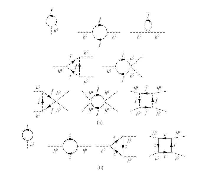
Figure 1: Generic diagrams contributing to the one-, two-, three- and four-point 1PI Green functions of the lightest Higgs boson $h^{0}$ at the one-loop level: a) with top-squark loops, $\tilde{f}\equiv\tilde{t}_{1},\tilde{t}_{2}$ , b) with top-quark loops.

The diagrams contributing to the $n$-point vertex functions $(n=1,...,4)$ from the top-quark/squark sector are shown generically in Fig. 1. The corresponding analytic expressions $\sim{\cal O}(m_{t}^{4})$, in the asymptotic limit according to (6)-(7), are given by

$$\Delta\Gamma_{h^{0}}^{t,\tilde{t}\,(1)} = \frac{3}{8\pi^{2}}\frac{g}{M_{W}}\,m_{t}^{4}\,\left(\Delta_{\epsilon}+1-\log\frac{m_{t}^{2}}{\mu_{0}^{2}}\right)\,,$$

$$\Delta\Gamma_{h^{0}}^{t,\tilde{t}\,(2)} = \frac{3}{16\pi^{2}}\frac{g^{2}}{M_{W}^{2}}\,m_{t}^{4}\,\left(\Delta_{\epsilon}+1+\log\frac{m_{\tilde{t}_{1}}^{2}}{\mu_{0}^{2}}+\log\frac{m_{\tilde{t}_{2}}^{2}}{\mu_{0}^{2}}-3\log\frac{m_{t}^{2}}{\mu_{0}^{2}}\right)\,,$$

$$\Delta\Gamma_{h^{0}}^{t,\tilde{t}\,(3)} = -\frac{3}{16\pi^{2}}\frac{g^{3}}{M_{W}^{3}}\,m_{t}^{4}\,\left(2+3\log\frac{m_{t}^{2}}{m_{\tilde{t}_{1}}m_{\tilde{t}_{2}}}\right)\,,$$

$$\Delta\Gamma_{h^{0}}^{t,\tilde{t}\,(4)} = -\frac{3}{32\pi^{2}}\frac{g^{4}}{M_{W}^{4}}\,m_{t}^{4}\,\left(8+3\log\frac{m_{t}^{2}}{m_{\tilde{t}_{1}}m_{\tilde{t}_{2}}}\right)\,,$$ (26)

where $\mu_{0}$ is the scale of dimensional regularization. All other terms depending on the external momenta and on the stop-mass splitting vanish for large values of $m_{\tilde{t}_{1,2}}$. The three- and four-point functions are UV-finite, whereas the one- and two-point functions involve a singular $\Delta_{\epsilon}$ term, with

$$\hskip 17.07182pt\displaystyle{\Delta}_{\epsilon}=\frac{2}{\epsilon}-{\gamma}_{\epsilon}+\log(4\pi)\hskip 5.69046pt,\hskip 5.69046pt\epsilon=4-D\,.$$ (27)

All these contributions contain a logarithmic dependence on the stop masses. These functions are the only remainder of a heavy stop system in the vertex functions of the $h^{0}$ and thus summarize all the potential non-decoupling effects of these particles in the effective potential for the lightest Higgs boson. At this point, one could be tempted to conclude that heavy top-squarks do not decouple in the Green functions of the lightest CP-even Higgs boson of the ${\rm MSSM}$ and therefore, in the $h^{0}$ self-couplings. It is essential, however, to study whether those effects appear in the relations between observables [36].

There are also non-logarithmic finite contributions to the three- and four-point functions in (3.1). These terms arise from the last two diagrams in Fig. 1. They are also present for the Higgs particle ($H_{{\rm SM}}$) in the external legs, instead of $h^{0}$. Therefore, they do not contribute to the difference between the $h^{0}$ and $H_{{\rm SM}}$ properties (see next section).

3.2 Renormalized vertices and decoupling behaviour

The vertex functions obtained from the set of one-loop diagrams are in general UV-divergent. For finite 1PI Green functions and physical observables, renormalization has to be performed by adding appropriate counterterms. For a systematic 1-loop calculation, the free parameters of the Higgs potential $m_{1}^{2},\,m_{2}^{2},\,m_{12}^{2},\,g,\,g^{\prime}$ and the two vacua $v_{1},\,v_{2}$ are replaced by renormalized parameters plus counterterms. This transforms the potential $V$ into $V+\delta V$, where V, expressed in terms of the renormalized parameters, is formally identical to (10), and $\delta V$ is the counterterm potential. By using the standard renormalization procedure [26, 9] with $m_{i}^{2}\rightarrow Z_{H_{i}}^{-1}(m_{i}^{2}+\delta m_{i}^{2})\,,$ $g\rightarrow Z_{1}^{W}Z_{2}^{W\,-\frac{3}{2}}g\,,$ $g^{\prime}\rightarrow Z_{1}^{B}Z_{2}^{B\,-\frac{3}{2}}g^{\prime}\,,$ $v_{i}\rightarrow Z_{H_{i}}^{1/2}(v_{i}-\delta v_{i})\,,$ and with field renormalization constants $\delta Z_{H_{i}}$, we obtain the counterterms for the $n$-point $(n=1,...,4)$ vertex functions in the decoupling limit as follows:

$$\delta\Gamma_{h^{0}}^{(1)} = \frac{gM_{Z}}{2c_{{\scriptscriptstyle W}}}\cos 2\beta v^{2}\left(\sin^{2}\beta\,\delta Z_{H_{2}}-\cos^{2}\beta\,\delta Z_{H_{1}}\right)-v\,\delta M_{12}^{2}$$

$$+ \frac{1}{4}\frac{g^{2}}{c_{{\scriptscriptstyle W}}^{2}}v^{2}\cos^{2}2\beta\,\delta v-\frac{1}{8}v^{3}\cos^{2}2\beta\,\delta G^{2}\,,$$

$$\delta\Gamma_{h^{0}}^{(2)} = \frac{3}{4}\left[v^{2}\cos 2\beta\,\frac{g^{2}}{c_{{\scriptscriptstyle W}}^{2}}\left(\sin^{2}\beta\,\delta Z_{H_{2}}-\cos^{2}\beta\,\delta Z_{H_{1}}\right)-\frac{4}{3}\,\delta M_{12}^{2}\right.$$

$$+ \left.\frac{g^{2}}{c_{{\scriptscriptstyle W}}^{2}}\cos^{2}2\beta\,v\,\delta v-\frac{v^{2}}{2}\cos^{2}2\beta\,\delta G^{2}\right]\,,$$

$$\delta\Gamma_{h^{0}}^{(3)} = \frac{3}{4}\cos 2\beta\left[2v\frac{g^{2}}{c_{{\scriptscriptstyle W}}^{2}}\left(\sin^{2}\beta\,\delta Z_{H_{2}}-\cos^{2}\beta\,\delta Z_{H_{1}}\right)-\frac{g^{2}}{c_{{\scriptscriptstyle W}}^{2}}\cos 2\beta\delta v-v\cos 2\beta\,\delta G^{2}\right],$$

$$\delta\Gamma_{h^{0}}^{(4)} = \frac{3}{4}\cos 2\beta\left[2\frac{g^{2}}{c_{{\scriptscriptstyle W}}^{2}}\left(\sin^{2}\beta\,\delta Z_{H_{2}}-\cos^{2}\beta\,\delta Z_{H_{1}}\right)-\cos 2\beta\,\delta G^{2}\right]\,,$$ (28)

where we have introduced the abbreviations

$$\delta G^{2} \equiv \delta g^{2}+\delta g^{\prime 2}=g^{2}(2\,\delta Z_{1}^{W}-3\,\delta Z_{2}^{W})-g^{\prime 2}\delta Z_{2}^{B}\,,$$

$$\delta M_{12}^{2} \equiv \cos^{2}\beta\,\delta m_{1}^{2}+\sin^{2}\beta\,\delta m_{2}^{2}+\sin 2\beta\,\delta m_{12}^{2}\,,$$

$$v\,\delta v = v_{1}\delta v_{1}+v_{2}\delta v_{2}\,\,\,{\mbox{with}}\,\,\,v^{2}=v_{1}^{2}+v_{2}^{2}\,.$$ (29)

In the same way, the pseudoscalar-mass counterterm is obtained as

$$\delta M_{A^{0}}^{2} = \frac{1}{2}\left(\sin^{2}\beta\,\delta m_{1}^{2}+\cos^{2}\beta\,\delta m_{2}^{2}-\sin 2\beta\,\delta m_{12}^{2}\right)$$ (30)

$$- \frac{1}{4}M_{Z}^{2}\cos^{2}2\beta\left(\frac{c_{{\scriptscriptstyle W}}^{2}}{g^{2}}\,\delta G^{2}+\delta Z_{H_{1}}+\delta Z_{H_{2}}-2\frac{\delta v}{v}\right)\,.$$

In the on-shell scheme, adopted in this paper, the counterterms are fixed by imposing the following renormalization conditions [9, 37]:
– the on-shell conditions for $M_{W,Z}$ and the electric charge $e$ as in the minimal ${\rm SM}$,
– the on-shell condition for the $A^{0}$ boson with the pole mass $M_{A}$,
– the tadpole conditions for vanishing renormalized tadpoles, i.e. the sum of the 1-loop tadpole diagrams for $H^{0}$, $h^{0}$, and the corresponding tadpole counterterm is equal to zero,
– the renormalization of $\tan\beta$ in such a way that the relation $\tan\beta=v_{2}/v_{1}$ is valid for the 1-loop Higgs minima.

By this set of conditions, the input for the ${\rm MSSM}$ Higgs sector is fixed by the pole mass $M_{A}$ and $\tan\beta$, together with the standard gauge-sector input $M_{W,Z}$ and $e$.

With restriction to the dominant ${\cal O}(m_{t}^{4})$ contributions, the mass and field counterterms appearing in (3.2)-(30) have the following structure:

$$\delta Z_{H_{1,2}}=0\,,\,\,\,\delta v=0\,,\,\,\,\delta G^{2}=0\,,$$

$$\delta M_{12}^{2}=\frac{3}{16\pi^{2}}\frac{g^{2}}{M_{W}^{2}}\,m_{t}^{4}\,\left(\Delta_{\epsilon}+1-\log\frac{m_{t}^{2}}{\mu_{0}^{2}}\right)\,,$$

$$\delta M_{A^{0}}^{2}=\frac{3}{16\pi^{2}}\frac{g^{2}}{M_{W}^{2}}\,m_{t}^{4}\,\cot^{2}\beta\,\left(\Delta_{\epsilon}+1-\log\frac{m_{t}^{2}}{\mu_{0}^{2}}\right)\,.$$ (31)

Now the renormalized vertex functions are obtained as the sum of the one-loop contributions in (3.1) and the counterterms (3.2) together with (3.2). The renormalized one-point function vanishes, according to the corresponding renormalization condition: $\Delta\Gamma_{h^{0}}^{\,t,\tilde{t}\,(1)}+\delta\Gamma_{h^{0}}^{\,t,\tilde{t}\,(1)}=0$.

The renormalized two-point function is given by

$$\Delta\Gamma_{h^{0}}^{\,t,\tilde{t}\,(2)}+\delta\Gamma_{h^{0}}^{\,t,\tilde{t}\,(2)}=-\frac{3}{8\pi^{2}}\frac{g^{2}}{M_{W}^{2}}\,m_{t}^{4}\,\log\frac{m_{t}^{2}}{m_{\tilde{t}_{1}}m_{\tilde{t}_{2}}}\,.$$ (32)

As expected, the UV-divergence cancels between the one-loop and the counterterm contributions; however, a logarithmic heavy mass term, which looks like a non-decoupling effect of the heavy particles, remains. The renormalized two-point function is responsible for a shift in the pole of the $h^{0}$ propagator and thus represents the (leading) one-loop correction to the $h^{0}$ mass,

$$\Delta M_{h^{0}}^{2}=-\frac{3}{8\pi^{2}}\frac{g^{2}}{M_{W}^{2}}\,m_{t}^{4}\,\log\frac{m_{t}^{2}}{m_{\tilde{t}_{1}}m_{\tilde{t}_{2}}}\,.$$ (33)

The same expression is obtained from the results listed in ref. [11] for the leading one-loop radiative corrections from the $t,\tilde{t}-$sector to the light $h^{0}$ boson for the special case of $M_{A}\gg M_{Z}$ and in the limiting situations defined in (7).

For the counterterms to the three- and four-point functions, there is no ${\cal O}(m_{t}^{4})$ contribution. Hence, the renormalized $h^{0}$ three- and four-point vertices, using the result (33), can be expressed as follows,

$$\Delta\Gamma_{h^{0}}^{\,t,\tilde{t}\,(3)}=\frac{3}{v}\,\Delta M_{h^{0}}^{2}-\frac{3}{8\pi^{2}}\frac{g^{3}}{M_{W}^{3}}\,m_{t}^{4}\,,$$

$$\Delta\Gamma_{h^{0}}^{\,t,\tilde{t}\,(4)}=\frac{3}{v^{2}}\,\Delta M_{h^{0}}^{2}-\frac{3}{4\pi^{2}}\frac{g^{4}}{M_{W}^{4}}\,m_{t}^{4}\,.$$ (34)

Without the non-logarithmic top-mass term, the trilinear and quartic $h^{0}$ self couplings at the one-loop level have the same form as in (24), with the tree-level Higgs mass replaced by the corresponding one-loop mass

$$M_{h^{0}}^{2}=M^{2\,{\mathrm{tree}}}_{h^{0}}+\Delta M_{h^{0}}^{2}\,.$$ (35)

The terms logarithmic in the heavy-squark masses disappear when the vertices are expressed in terms of the Higgs-boson mass $M_{h^{0}}$ and, therefore, they do not appear directly in related observables, i.e. they decouple. Moreover, the $h^{0}$ self-couplings get the form of the self-couplings of the SM Higgs boson (9) with $M_{H}=M_{h^{0}}$. The non-logarithmic top-mass terms are common to both $h^{0}$ and $H_{SM}$ (in the SM after renormalization of the trilinear and quartic couplings).

To make this last point explicit, we give the one-loop ${\cal O}(m_{t}^{4})$ contributions for the SM Higgs $n$-point vertex functions, which follow from the last four diagrams in Figure 1 (with $H\equiv H_{{\rm SM}}$ instead of $h^{0}$ in the external lines)

$$\Delta\Gamma_{H}^{(1)}=\frac{3g}{8\pi^{2}M_{W}}\,m_{t}^{4}\left(\Delta_{\epsilon}-\log\frac{m_{t}^{2}}{\mu_{0}^{2}}+1\right)\,,$$

$$\Delta\Gamma_{H}^{(2)}=\frac{3g^{2}}{16\pi^{2}M_{W}^{2}}\,m_{t}^{4}\left(3\,\Delta_{\epsilon}-3\log\frac{m_{t}^{2}}{\mu_{0}^{2}}+1\right)\,,$$

$$\Delta\Gamma_{H}^{(3)}=\frac{3g^{3}}{16\pi^{2}M_{W}^{3}}\,m_{t}^{4}\left(3\,\Delta_{\epsilon}-3\log\frac{m_{t}^{2}}{\mu_{0}^{2}}-2\right)\,,$$

$$\Delta\Gamma_{H}^{(2)}=\frac{3g^{4}}{32\pi^{2}M_{W}^{4}}\,m_{t}^{4}\left(3\,\Delta_{\epsilon}-3\log\frac{m_{t}^{2}}{\mu_{0}^{2}}-8\right)\,.$$ (36)

Differently from the MSSM $h^{0}$ boson, the 3- and 4-point SM vertices are not UV-finite and require renormalization also at the level of the ${\cal O}(m_{t}^{4})$ approximation. Adding the counterterms, which are derived from the SM Higgs potential

$$V=-\frac{\mu^{2}}{2}\,(v+H)^{2}+\frac{\lambda}{4}\,(v+H)^{4}$$ (37)

via ${\rm SM}$ parameter renormalization ($\lambda\rightarrow\lambda+\delta\lambda$, $\mu^{2}\rightarrow\mu^{2}+\delta\mu^{2}$, $v\rightarrow v-\delta v$), yields the renormalized one-loop vertex functions

$$\Delta\hat{\Gamma}_{H}^{(1)}=\Delta\Gamma_{H}^{(1)}+\delta\Gamma_{H}^{(1)}\,=\,\Delta\Gamma_{H}^{(1)}+v^{3}\delta\lambda-v\delta\mu^{2}-(3v^{2}\lambda-\mu^{2})\,\delta v\,,$$

$$\Delta\hat{\Gamma}_{H}^{(2)}=\Delta\Gamma_{H}^{(2)}+\delta\Gamma_{H}^{(2)}\,=\,\Delta\Gamma_{H}^{(2)}+3v^{2}\delta\lambda-\delta\mu^{2}-6v\lambda\,\delta v\,,$$

$$\Delta\hat{\Gamma}_{H}^{(3)}=\Delta\Gamma_{H}^{(3)}+\delta\Gamma_{H}^{(3)}\,=\,\Delta\Gamma_{H}^{(3)}+6v\,\delta\lambda-6\lambda\,\delta v\,,$$

$$\Delta\hat{\Gamma}_{H}^{(4)}=\Delta\Gamma_{H}^{(4)}+\delta\Gamma_{H}^{(4)}\,=\,\Delta\Gamma_{H}^{(4)}+6\,\delta\lambda\,.$$ (38)

The renormalization constant $\delta v$ is determined from the gauge sector and has no ${\cal O}(m_{t}^{4})$ contribution, i.e. $\delta v=0$. The other renormalization constants $\delta\mu^{2}$ and $\delta\lambda$ have to be determined from the renormalization in the Higgs sector. The corresponding two on-shell conditions are:
– Tadpole condition:                   $\Delta\hat{\Gamma}_{H}^{(1)}\,=\,0\,,$
– Higgs mass renormalization: $\quad\Delta\hat{\Gamma}_{H}^{(2)}\,=\,0\,.$
Solving these equations yields

$$\delta\lambda\,=\,\frac{1}{2v^{2}}\left(\Delta\Gamma_{H}^{(2)}-\frac{1}{v}\Delta\Gamma_{H}^{(1)}\right)\,=\,\frac{3g^{4}}{64\pi^{2}M_{W}^{4}}\,m_{t}^{4}\left(\Delta_{\epsilon}-\log\frac{m_{t}^{2}}{\mu_{0}}\right)\,,$$ (39)

with the expressions in (3.2) and with $v=2M_{W}/g$. Finally, according to (3.2), one finds for the renormalized 3- and 4-point vertices

$$\Delta\hat{\Gamma}_{H}^{(3)}=-\frac{3g^{3}}{8\pi^{2}M_{W}^{3}}\,m_{t}^{4}\,,\quad\quad\Delta\hat{\Gamma}_{H}^{(4)}=-\frac{3g^{4}}{4\pi^{2}M_{W}^{4}}\,m_{t}^{4}\,,$$ (40)

which correspond precisely to the two non-logarithmic terms in (3.2).

To summarize this section, we conclude that all the ${\cal O}(m_{t}^{4})$ one-loop ${\rm MSSM}$ contributions to the $h^{0}$ Green functions in the asymptotic limit either represent a shift in the $h^{0}$ mass and in the $h^{0}$ triple and quartic self-couplings, which can be absorbed in $M_{h^{0}}$, or reproduce the SM top-loop corrections. The triple and quartic $h^{0}$ couplings thereby acquire the structure of the SM Higgs-boson self-couplings. Heavy top squarks thus decouple from the low energy theory when the self-couplings are expressed in terms of the Higgs-boson mass.

4 Trilinear and quartic $h^{0}$ self-couplings

In the previous section, the results for the one-loop contributions to the three- and four-point functions were discussed considering in the Higgs sector the decoupling limit and in the squark ${\rm MSSM}$ sector the limit of heavy $\tilde{t}$ masses compared to the electroweak scale, such that $\tilde{t}_{1}$ and $\tilde{t}_{2}$ have masses very close to each other (cf. (7)). In this section we study the more general case assuming only that the stop masses are very heavy compared to the electroweak scale (see eq. (6)), but without further assumptions on the relative size of the top-squark masses. Moreover, also the requirement of the decoupling limit in the Higgs sector is released. A numerical discussion for the trilinear coupling shows how fast and to which accuracy the asymptotic results are achieved, for the cases specified in (7) and (8). The numerical analysis of the trilinear self-coupling is appropriately extended also to the quartic $h^{0}$ self-coupling.

Following the decomposition (25), we write the trilinear self-coupling of the $h^{0}$ boson as a sum of the tree-level coupling and the one-loop radiative correction,

$$\lambda_{hhh}=\lambda_{hhh}^{0}+\Delta\lambda_{hhh}=\lambda_{hhh}^{0}\left(1+\frac{\Delta\lambda_{hhh}}{\lambda_{hhh}^{0}}\right)\,,$$ (41)

where $h\equiv h^{0}$ and $\lambda_{hhh}^{0}$ is defined in (2.2); $\Delta\lambda_{hhh}$ is the renormalized one-loop three-point vertex,

$$\Delta\lambda_{hhh}=\Delta\Gamma_{h^{0}}^{t,\tilde{t}\,(3)}\,+\,\delta\Gamma_{h^{0}}^{\,t,\tilde{t}\,(3)}\,,$$ (42)

and, accordingly, in similar notation for the quartic coupling.

Concerning the analytic expression for the one-loop ${\cal O}(m_{t}^{4})$ correction $\Delta\lambda_{hhh}$, from the $t,\tilde{t}$-sector, we find the result already given in [14] (for $M_{\tilde{Q}}=M_{\tilde{U}}$ also in [15]), which can be written in a compact form,

$$\Delta\lambda_{hhh} = \frac{3g^{3}}{32\pi^{2}}\frac{1}{M_{W}^{3}}\,m_{t}^{4}\,\frac{\cos^{3}\alpha}{\sin^{3}\beta}$$ (43)

$$\times \left\{3\log\frac{m_{\tilde{t}_{1}}^{2}m_{\tilde{t}_{2}}^{2}}{m_{t}^{4}}+3(m_{\tilde{t}_{1}}^{2}-m_{\tilde{t}_{2}}^{2})\,C_{t}F_{t}\log\frac{m_{\tilde{t}_{1}}^{2}}{m_{\tilde{t}_{2}}^{2}}\right.$$

$$+\left.2\left(\frac{m_{t}^{2}}{m_{\tilde{t}_{1}}^{2}}\left[1+(m_{\tilde{t}_{1}}^{2}-m_{\tilde{t}_{2}}^{2})\,C_{t}F_{t}\right]^{3}+\frac{m_{t}^{2}}{m_{\tilde{t}_{2}}^{2}}\left[1-(m_{\tilde{t}_{1}}^{2}-m_{\tilde{t}_{2}}^{2})\,C_{t}F_{t}\right]^{3}-2\right)\right.$$

$$+ \left.3\left(\frac{M_{\tilde{Q}}^{2}-M_{\tilde{U}}^{2}}{m_{\tilde{t}_{1}}^{2}-m_{\tilde{t}_{2}}^{2}}\right)^{2}\left[(m_{\tilde{t}_{1}}^{2}-m_{\tilde{t}_{2}}^{2})F_{t}^{2}\log\frac{m_{\tilde{t}_{1}}^{2}}{m_{\tilde{t}_{2}}^{2}}+(m_{\tilde{t}_{1}}^{2}-m_{\tilde{t}_{2}}^{2})^{2}C_{t}F_{t}^{3}g_{t}\right]\right\},$$

with

$$C_{t} = X_{t}\,/\,(m_{\tilde{t}_{1}}^{2}-m_{\tilde{t}_{2}}^{2})\,,\,\,{\mbox{ with }}\,X_{t}{\mbox{ defined in }}(\ref{eq:MLRtb})\,,$$

$$F_{t} = (A_{t}+\mu\tan\alpha)/(m_{\tilde{t}_{1}}^{2}-m_{\tilde{t}_{2}}^{2})\,,$$

$$g_{t} = 2-\frac{m_{\tilde{t}_{1}}^{2}+m_{\tilde{t}_{2}}^{2}}{m_{\tilde{t}_{1}}^{2}-m_{\tilde{t}_{2}}^{2}}\log\frac{m_{\tilde{t}_{1}}^{2}}{m_{\tilde{t}_{2}}^{2}}\,.$$ (44)

Notice that the non-logarithmic finite contributions to the three-point function from the top-triangle diagram in Fig. 1 is also included in (43) (the term with $-2$ in the third line of (43)). It is, however, not taken into account in the figures since it converges always to the ${\rm SM}$ term.

By considering the decoupling limit, which implies $\cos\alpha\rightarrow\sin\beta$, $\tan\alpha\rightarrow-\cot\beta$, and by doing the appropriate expansion in (43) for the assumptions given in (6), (7), one recovers the asymptotic expression for the three-point function given in (3.1). In order to illustrate also quantitatively how the results given in (3.1) and (43) are approached in the asymptotic limit of $\Delta\lambda_{hhh}$, we plot in Fig. 2 the ratio $\Delta\lambda_{hhh}/\lambda_{hhh}^{0}$ as function of $M_{A^{0}}$ and $\tan\!\beta$, choosing values of the parameters which obey strictly the asymptotic conditions (7) for the squark sector:

$$M_{\tilde{Q}}\sim M_{\tilde{U}}\sim 15{\mbox{ TeV}}\,,\,\,\,\,\,\,\mu\sim|A_{t}|\sim 1.5{\mbox{ TeV}}\,.$$ (45)

For definiteness, we also list the following values used for the SM parameters along all figures in this paper: $G_{F}=1.16639\times 10^{-5}$, $m_{t}=175\,{\rm GeV}$, $m_{b}=4.62\,{\rm GeV}$, $M_{Z}=91.188\,{\rm GeV}$, $M_{W}=80.41\,{\rm GeV}$ [38].

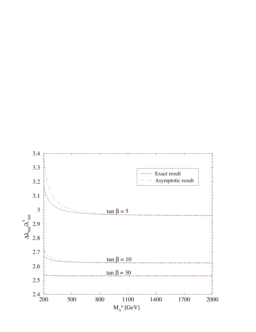
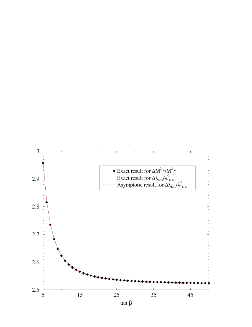
(a)	(b)

Figure 2: Exact and asymptotic result of ${\cal O}(m_{t}^{4})$ for a) ${\Delta\lambda_{hhh}}/{\lambda_{hhh}^{0}}$ $\scriptstyle{(h\equiv h^{0})}$ as a function of $M_{A^{0}}$ and b) ${\Delta\lambda_{hhh}}/{\lambda_{hhh}^{0}}$ and ${\Delta M_{h^{0}}^{2}}/{M_{h^{0}}^{2}}$ as a function of $\tan\!\beta$, for $M_{A^{0}}=1$ TeV. The SUSY parameters have been chosen as in (45).

In Fig. 2a the variation of the trilinear coupling with $M_{A^{0}}$ is shown for different values of $\tan\!\beta$. Clearly, the asymptotic and exact results are in agreement for large $M_{A^{0}}$ values, above 500 GeV, depending in detail on $\tan\!\beta$. An explicit numerical evaluation of $\Delta\lambda_{hhh}/\lambda_{hhh}^{0}$ as a function of $\tan\!\beta$ is presented in Fig. 2b. The $A$-boson mass $M_{A^{0}}=1$ TeV corresponds already to the decoupling limit of the Higgs sector, and the various results for the triple coupling coincide. In order to illustrate how well the radiative corrections to $\Delta\lambda_{hhh}$ can be described in terms of the corresponding shift in $M_{h^{0}}$, asymptotically given in (3.2), we also display the variation of $\Delta M_{h^{0}}^{2}/{M^{2\,{\mathrm{tree}}}_{h^{0}}}$ in this figure. $\Delta M_{h^{0}}^{2}/{M^{2\,{\mathrm{tree}}}_{h^{0}}}$ is represented by black diamonds; it has been obtained according to the ${\cal O}(m_{t}^{4})$ one-loop Higgs-boson mass results presented in [9]. The agreement with the vertex corrections is clearly visible. Therefore, the radiative corrections to $\lambda_{hhh}$, although large, disappear when $\lambda_{hhh}$ is expressed in terms of $M_{h^{0}}$.

So far we have concentrated on the trilinear $h^{0}$ self-coupling, and we did not give explicite results for the quartic Higgs boson self-coupling. The analytic expressions are quite lengthy and hence we do not list them here. Numerically, the higher-order contribution to the quartic coupling, $\Delta\lambda_{hhhh}$, normalized to the tree-level value $\lambda_{hhhh}^{0}$ in (24), show the same behaviour as the triple coupling in Fig. 2 (since the differences are marginal, we do not include an extra figure). This is also a numerical proof that the ${\cal O}(m_{t}^{4})$ corrections to the quartic $h^{0}$ self-coupling are absorbed in the $h^{0}$ mass in the asymptotic limit.

For the rest of the analysis, we will consider the limiting situation in the squark sector that was specified in (8). In Fig. 3 we present numerical results for the variation of the trilinear coupling, given by the expression (43), and for the ${\cal O}(m_{t}^{4})$ $h^{0}$ mass correction, as given in [9], with $M_{A^{0}}$ and $\tan\!\beta$. The radiative correction to the angle $\alpha$ [9] is also taken into account. The SUSY parameters have been taken to be

$$M_{\tilde{Q}}\sim 1{\mbox{ TeV}}\,,\,\,\,\,\,\,M_{\tilde{U}}\sim\mu\sim|A_{t}|\sim 500{\mbox{ GeV}}\,.$$ (46)

With this choice of the ${\rm SUSY}$ parameters, the top-squark masses, $m_{\tilde{t}_{1}}$ and $m_{\tilde{t}_{2}}$, are heavy as compared to the to the electroweak scale, but their difference is of ${\cal O}(M_{\tilde{U}})$.

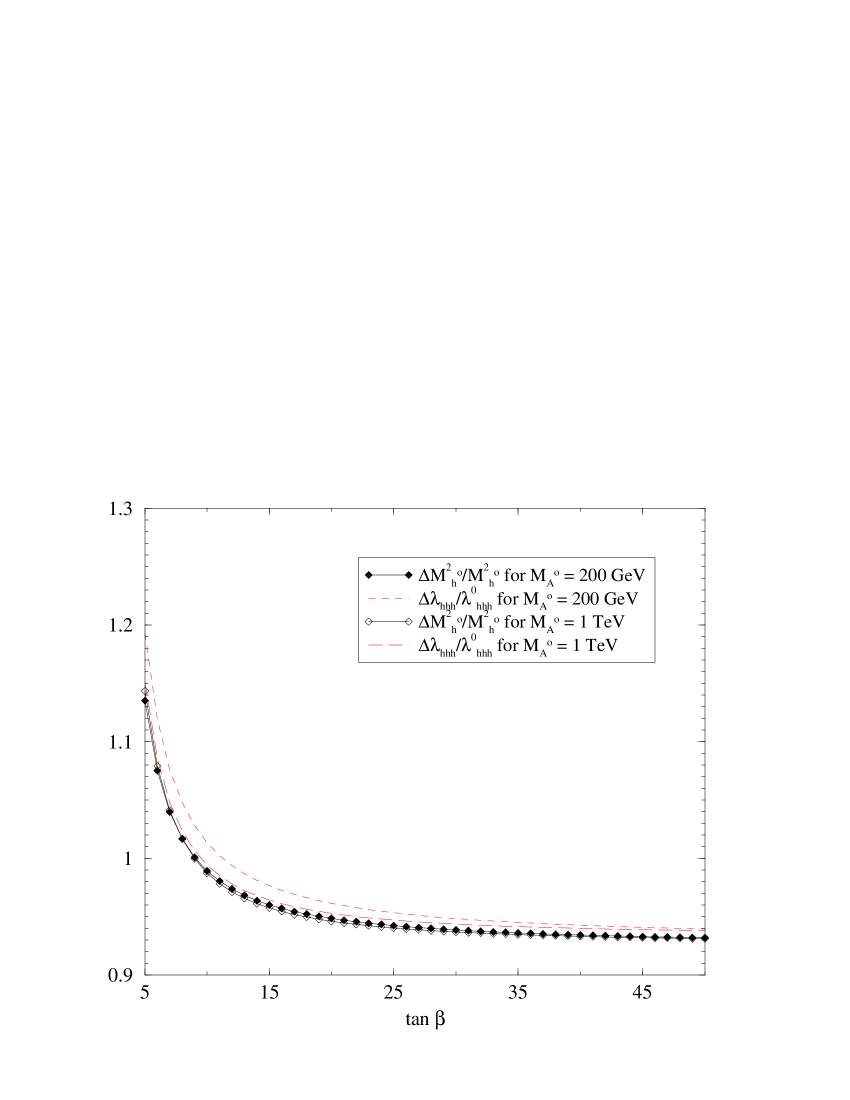
(a)	(b)

Figure 3: Leading Yukawa radiative corrections ${\cal O}(m_{t}^{4})$ to the trilinear $h^{0}$ self-coupling and to the $h^{0}$ mass as a function of a) $M_{A^{0}}$, and b) $\tan\!\beta$, for choices of the SUSY parameters as in (46).

Fig. 3a contains the variation of the trilinear coupling with $M_{A^{0}}$, for different values of $\tan\!\beta$. We also give in Fig. 3 the ${\cal O}(m_{t}^{4})$ corrections to $\Delta M_{h^{0}}^{2}/{M^{2\,{\mathrm{tree}}}_{h^{0}}}$ in order to point out how far the large radiative corrections to the $h^{0}$ self-coupling can be absorbed in the $h^{0}$ mass correction, $\Delta M_{h^{0}}^{2}$. The relation $\Delta\lambda_{hhh}/{\lambda_{hhh}^{0}}\approx\Delta M_{h^{0}}^{2}/{M^{2\,{\mathrm{tree}}}_{h^{0}}}$ is only fulfilled up to a small difference which remains also for large $M_{A}$. But even in the most unfavorable cases, namely low $\tan\!\beta$ and $M_{A^{0}}$ values, the difference between the $h^{0}$ mass and self-coupling at one-loop does not exceed $6\%$ (for $\tan\!\beta=5$ and $M_{A^{0}}=200$ GeV, it is about $\sim 5\%$). The difference decreases for larger values of $\tan\!\beta$; e.g. for $\tan\!\beta=10$ and $M_{A^{0}}=200$ GeV, the mass and self-coupling corrections are equal within $\sim 2\%$. This is more explicitely displayed in Fig. 3b, containing the variation of $\Delta\lambda_{hhh}/{\lambda_{hhh}^{0}}$ and $\Delta M_{h^{0}}^{2}/{M^{2\,{\mathrm{tree}}}_{h^{0}}}$ with $\tan\!\beta$ for $M_{A^{0}}=200$ GeV and $M_{A^{0}}=1$ TeV.

Therefore, from the numerical analysis one can conclude that also for the case of a heavy stop system with large mass splitting, of the order as the typical SUSY scale, the ${\cal O}(m_{t}^{4})$ corrections to the trilinear $h^{0}$ self-couplings are absorbed to a large extent in the loop-induced shift of the $h^{0}$ mass, leaving a small difference of only a few per cent, which can be interpreted as the genuine one-loop corrections when $\lambda_{hhh}$ is expressed in terms of $M_{h^{0}}$. Similar results have been obtained also for the quartic $h^{0}$ self-coupling, which again are close to the ones displayed in Fig. 3 and hence are not given in an extra figure.

5 Conclusions

The ${\cal O}(m_{t}^{4})$ corrections from the $t,\tilde{t}$-sector to the self-couplings of the light CP-even Higgs-boson in the ${\rm MSSM}$ have been evaluated. We showed analytically that, in the limit of large $M_{A^{0}}$ and heavy top squarks, with $m_{\tilde{t}_{1}}$ and $m_{\tilde{t}_{2}}$ close to each other, all the apparent non-decoupling one-loop effects, which constitute large corrections to the $h^{0}$ self-couplings, are absorbed in the Higgs-boson mass $M_{h^{0}}$, and the $h^{0}$ self-couplings get the same form as the couplings of the SM Higgs boson. Therefore, such a heavy top-squark system decouples from the low energy theory, at the electroweak scale, and leaves behind the SM Higgs sector also in the Higgs self-interactions.

Other limiting situations where the $\tilde{t}$-mass difference is of the order of the ${\rm SUSY}$ mass scale have also been investigated. Similarly to the previous limit, the radiative corrections to the $h^{0}$ self-couplings are large, but their main part can again be absorbed in the mass $M_{h^{0}}$. The genuine loop corrections to the triple and quartic couplings, after re-expressing them in terms of $M_{h^{0}}$, is of the order of a few per cent. They are largest for low $\tan\!\beta$ and $M_{A^{0}}$, with typically 5%. For large $M_{A^{0}}$, i.e. in the decoupling limit of the MSSM Higgs sector, they decrease to the level of 1%. The $h^{0}$ self-interactions are thus very close to those of the SM Higgs boson and would need high-precision experiments for their experimental verification.

References

• [1] H.P. Nilles, Phys. Rep. 110 (1984) 1;
H.E. Haber, G. Kane, Phys. Rep. 117 (1985) 75;
J. F. Gunion, H. E. Haber, Nucl. Phys. B272, 1 (1986); B278, 449 (1986), Erratum-ibid. B402, 567 (1993).
• [2] J. Ellis, talk at the XX International Symposium on Lepton and Photon Interactions at High Energies, Rome, July 2001 (to appear in the Proceedings);
F. Zwirner, talk at the XX International Symposium on Lepton and Photon Interactions at High Energies, Rome, July 2001 (to appear in the Proceedings);
G. Altarelli, F. Caravaglios, G.F. Giudice, P. Gambino, G. Ridolfi, hep-ph/0106029, JHEP 0106 (2001) 018
• [3] J. F. Gunion, H. E. Haber, G. Kane, S. Dawson, The Higgs Hunter’s Guide (Addison-Wesley, 1990), Erratum hep-ph/9302272.
• [4] J. A. Aguilar-Saavedra et al., ECFA/DESY LC Physics Working Group Collaboration, TESLA Technical Design Report, DESY 2001-011, ECFA-2001-209, hep-ph/0106315; T. Abe et al., American Linear Collider Working Group Collaboration, SLAC-R-570, hep-ex/0106056.
• [5] J. Ellis, G. Ridolfi, F. Zwirner, Phys. Lett. B257 (1991) 83; ibid. B262 (1991) 477;
Y. Okada, M. Yamaguchi, T. Yanagida, Prog. Theor. Phys.  85 (1991) 1;
H. E. Haber, R. Hempfling, Phys. Rev. Lett.  66 (1991) 1815.
• [6] R. Barbieri, M. Frigeni, F. Caravaglios, Phys. Lett. B258 (1991) 167;
R. Barbieri, M. Frigeni, Phys. Lett. B258 (1991) 395;
J. R. Espinosa, M. Quiros, Phys. Lett. B266 (1991) 389;
H. E. Haber, R. Hempfling, Phys. Rev. D48 (1993) 4280, hep-ph/9307201;
J. A. Casas, J. R. Espinosa, M. Quiros, A. Riotto, Nucl. Phys. B436 (1995) 3, Erratum-ibid. B439 (1995) 466, hep-ph/9407389;
M. Carena, J. R. Espinosa, M. Quiros, C. E. Wagner, Phys. Lett. B355 (1995) 209, hep-ph/9504316.
• [7] R. Hempfling, A. H. Hoang, Phys. Lett. B331 (1994) 99, hep-ph/9401219;
M. Carena, M. Quiros, C. E. Wagner, Nucl. Phys. B461 (1996) 407, hep-ph/9508343;
H. E. Haber, R. Hempfling, A. H. Hoang, Z. Phys. C75 (1997) 539, hep-ph/9609331;
J. A. Casas, J. R. Espinosa, H. E. Haber, Nucl. Phys. B526 (1998) 3, hep-ph/9801365;
R. Zhang, Phys. Lett. B447 (1999) 89, hep-ph/9808299;
J. R. Espinosa, R. Zhang, JHEP 0003 (2000) 026, hep-ph/9912236;
J. R. Espinosa, I. Navarro, hep-ph/0104047;
G. Degrassi, P. Slavich, F. Zwirner, hep-ph/0105096.
• [8] P. H. Chankowski, S. Pokorski and J. Rosiek, Phys. Lett. B274 (1992) 191;
A. Brignole, Phys. Lett. B281 (1992) 284;
D. M. Pierce, J. A. Bagger, K. Matchev, R. Zhang, Nucl. Phys. B491 (1997) 3, hep-ph/9606211.
• [9] A. Dabelstein, Z. Phys. C67 (1995) 495, hep-ph/9409375; Nucl. Phys. B456 (1995) 25, hep-ph/9503443.
• [10] S. Heinemeyer, W. Hollik, G. Weiglein, Acta Phys. Polon. B30 (1999) 1985, hep-ph/9903504; Eur. Phys. J.  C9 (1999) 343, hep-ph/9812472; Phys. Lett. B440 (1998) 296, hep-ph/9807423; Phys. Rev. D58 (1998) 091701, hep-ph/9803277; Comput. Phys. Commun.  124 (2000) 76, hep-ph/9812320.
• [11] S. Heinemeyer, W. Hollik, G. Weiglein, Phys. Lett. B455 (1999) 179, hep-ph/9903404.
• [12] M. Carena et al., Nucl. Phys. B580 (2000) 29, hep-ph/0001002.
• [13] S. Heinemeyer, W. Hollik, G. Weiglein, Eur. Phys. C16 (2000) 139, hep-ph/0003022;
S. Heinemeyer, W. Hollik, J. Rosiek, G. Weiglein, Eur. Phys. C19 (2001) 535, hep-ph/0102081.
• [14] V. Barger, M. S. Berger, A. L. Stange, R. J. Phillips, Phys. Rev. D45 (1992) 4128.
• [15] P. Osland, P. N. Pandita, Phys. Rev. D59 (1999) 055013, hep-ph/9806351; hep-ph/9911295; hep-ph/9902270.
• [16] A. Djouadi, W. Kilian, M. Mühlleitner, P. M. Zerwas, Eur. Phys. J. C10 (1999) 27, hep-ph/9903229; hep-ph/0001169; Eur. Phys. J. C10 (1999) 45, hep-ph/9904287;
M. Mühlleitner, hep-ph/0101262; hep-ph/0008127.
• [17] A. Djouadi, H. E. Haber, P. M. Zerwas, Phys. Lett. B375 (1996) 203, hep-ph/9602234.
• [18] T. Plehn, M. Spira, P. M. Zerwas, Nucl. Phys. B479 (1996) 46, Erratum-ibid. B531 (1996) 655, hep-ph/9603205; R. Lafaye, D. J. Miller, M. Mühlleitner, S. Moretti, hep-ph/0002238.
• [19] A. Dobado, M. J. Herrero, W. Hollik, S. Peñaranda, KA-TP-25-2001, in preparation.
• [20] M. Drees, K. Hagiwara, Phys. Rev. D42 (1990) 1709.
• [21] J.A. Coarasa, R.A. Jiménez, J. Solà, Phys. Lett. B389 (1996) 312, hep-ph/9511402;
J.A. Coarasa et al., Eur. Phys. J. C2 (1998) 373, hep-ph/9607485.
• [22] L.J. Hall, R. Rattazzi, U. Sarid, Phys. Rev. D50 (1994) 7048, hep-ph/9306309;
M. Carena, M. Olechowski, S. Pokorski, C.E.M. Wagner, Nucl. Phys. B426 (1994) 269, hep-ph/9402253;
M. Carena, S. Mrenna, C.E.M. Wagner, Phys. Rev. D60 (1999) 075010, hep-ph/9808312; ibid. D62 (2000) 055008, hep-ph/9907422;
M. Carena, D. Garcia, U. Nierste, C.E.M. Wagner, Nucl. Phys.  B577 (2000) 88, hep-ph/9912516.
• [23] H.E. Haber et al., Phys. Rev.  D63 (2001) 055004, hep-ph/0007006.
• [24] H. E. Haber et al., hep-ph/0102169;
M. J. Herrero, S. Peñaranda, D. Temes, Phys. Rev. D64 (2001) 115003, hep-ph/0105097.
• [25] J. Guasch, W. Hollik, S. Peñaranda, Phys. Lett. B515 (2001) 367, hep-ph/0106027.
• [26] P. H. Chankowski et al., Nucl. Phys. B417 (1994) 101;
P. Chankowski, S. Pokorski and J. Rosiek, Nucl. Phys.  B423 (1994) 437, hep-ph/9303309.
• [27] P. Gosdzinsky, J. Solà, Phys. Lett. B254 (1991) 139;
D. Garcia, J. Solà, Mod. Phys. Lett. A9 (1994) 211;
D. Garcia, R. A. Jiménez, J. Solà, Phys. Lett. B347 (1995) 309, hep-ph/9410310; ibid. B347 (1995) 321, hep-ph/9410311; Erratum-ibid. B351, 602 (1995);
S. Alam et al., Phys. Rev.  D62 (2000) 095011, hep-ph/0002066;
A. Belyaev, D. Garcia, J. Guasch, J. Solà, hep-ph/0105053.
• [28] A. Djouadi, V. Driesen, W. Hollik, J. I. Illana, Eur. Phys. J. C1 (1998) 149, hep-ph/9612362.
• [29] M. Carena, H. E. Haber, H. E. Logan, S. Mrenna, hep-ph/0106116;
A. M. Curiel, M. J. Herrero, D. Temes, J. F. Troconiz, hep-ph/0106267;
A. Dobado, M. J. Herrero, D. Temes, hep-ph/0107147.
• [30] A. Dobado, M. J. Herrero, S. Peñaranda, Eur. Phys. J. C7 (1999) 313, hep-ph/9710313; Eur. Phys. J. C12 (2000) 673, hep-ph/9903211; Eur. Phys. J. C17 (2000) 487, hep-ph/0002134.
• [31] A. Dobado, M. J. Herrero, S. Peñaranda, in: Proceedings of the Workshop on Quantum effects in the minimal supersymmetric standard model, Barcelona 1997, ed. J. Solà, World Scientific 1998 [hep-ph/9711441]; Contribution to the 29th International Conference on High-Energy Physics, Vancouver 1998, FTUAM-98-1, hep-ph/9806488.
• [32] H. E. Haber, hep-ph/9305248. Proceedings of the 23rd Workshop on the INFN Eloisatron Project, The Decay Properties of SUSY Particles, Erice 1992 (p. 321-372).
• [33] T. Hahn, M. Pérez-Victoria, Comput. Phys. Commun.  118 (1999) 153, hep-ph/9807565;
T. Hahn, hep-ph/0012260; T. Hahn, C. Schappacher, hep-ph/0105349.
• [34] G. ’t Hooft, M. Veltman, Nucl. Phys. B153 (1979) 365;
G. Passarino, M. Veltman, Nucl. Phys. B160 (1979) 151.
• [35] M. Capdequi Peyranere, H. E. Haber, P. Irulegui, Phys. Rev. D44 (1991) 191.
• [36] T. Appelquist, J. Carazzone, Phys. Rev. D11 (1975) 2856.
• [37] M. Böhm, H. Spiesberger, W. Hollik, Fortsch. Phys.  34 (1986) 687;
W. Hollik, Fortsch. Phys.  38 (1990) 165.
• [38] D. E. Groom et al. [Particle Data Group Collaboration], Eur. Phys. J.  C15 (2000) 1.