NEUTRINO OSCILLATIONS IN EXTRA DIMENSIONS

The characteristics and phenomenology of neutrino oscillation in extra dimensions are briefly reviewed

1 Introduction

The spacetime as we know it is four dimensional. A fifth dimension was postulated by Kaluza and Klein (KK) $\!{}^{{\bf?}}$ in the 1920’s, in an attempt to unify electromagnetism and gravity. If a fifth dimension exists, it must be very small or else it would have been seen. To estimate how small that is, recall that the allowed wave numbers in the fifth dimension are integral multiples of $1/R$, the inverse radius of that extra dimension. Excited wave numbers are seen as massive particles in our four-dimensional world, with a mass gap $1/R$. Since no such KK particles are known up to about 1 TeV, the radius $R$ must be smaller than 1 (TeV)${}^{-1}=2\times 10^{-19}$ m. This is the picture of the fifth dimension until a few years ago.

Recently a different view emerged $\!{}^{{\bf?}}$ which allows the extra dimensions to be large. Partly motivated by the discovery of D-branes in string theory $\!{}^{{\bf?}}$, it postulates all Standard Model (SM) particles to be permanently confined to our four-dimensional world, the so-called ‘3-brane’. Being confined they can have no KK excitations, so the previous bound on $R$ is no longer valid. On the other hand, SM singlets such as gravity and right-handed neutrinos are allowed to wander into the extra-dimensional world, ‘the bulk’. As a consequence, the inverse-square law of gravitational force is modified at separations less than $R$. Such a deviation has not been detected down to submillimeter separations $\!{}^{{\bf?}}$, from which we obtain an upper bound of $R$ to be about $10^{-4}$ m, not the much smaller $10^{-19}$ m discussed before. Moreover, if there are $n$ extra dimensions, the fundamental energy scale will change from $M_{P}\sim 10^{19}$ GeV to $M_{f}=[M_{P}^{2}/(2\pi R)^{n}]^{1/(n+2)}$. For $n=2$ and $R=0.4$ mm, this can be as low as 1 TeV, leading to many observable consequences. However, if $n=1$, $M_{f}=2.3\times 10^{8}$ GeV remains quite beyond our present capability to reach, then neutrino physics is probably the only way to detect the extra dimension. This is why neutrino physics is so important and so interesting in this connection. In this talk I will discuss some of the consequences for neutrino oscillation when there is only one large extra dimension present. The small extra dimensions decouple and will not be taken into account. For simplicity I will assume the fifth dimension to be flat, though a curved scenario is also interesting $\!{}^{{\bf?}}$.

2 Neutrinos Are Different

Neutrino is unique as an extra-dimensional probe because the right-handed neutrino is a SM singlet. A large radius $R$ in the extra dimension creates a small energy scale $1/R$ that only neutrinos can see, which may be why neutrinos have such exceptionally small masses. For $R=0.4$ mm, the energy $1/R$ is half a millivolt. Whether this is really the natural energy scale is unimportant for what follows because I will treat the neutrino masses as parameters.

A right-handed neutrino roaming in the bulk is derived from a 5-dimensional Dirac field, and is sterile. It gives rise to a KK tower of left-handed and right-handed neutrinos. The minimum content of a five-dimensional theory consists of three active brane neutrinos and a sterile bulk neutrino. Depending on the model, there may of course be more brane neutrinos which are sterile, and/or more bulk neutrinos.

Quark mixing via the CKM matrix is small, but at least some of the mixings for active neutrinos is large. One might be able to expalin this difference if the additional amount of neutrino mixing is derived from their coupling to the bulk neutrino(s).

In the presence of a bulk neutrino in a large extra dimension, neutrino oscillations possess special characteristics. The infinite number of states in the KK tower generally leads to a very complicated oscillation pattern. Besides, these neutrinos are sterile so they have neither charge nor neutral current interactions with matter. These are features detectable from neutrino oscillation experiments.

I will discuss two simple models $\!{}^{{\bf?},{\bf?}}$ in some detail to illustrate these characteristics. These models are instructive though possibly too simple to be realistic. I will also discuss more complicated models later in the section on phenomenology.

3 Mixings and Oscillations

Before discussing these models let me first review the usual formalism of neutrino oscillations. Let $\nu_{e},\nu_{\mu},\nu_{\tau}$ be the active neutrinos in the flavor basis, namely, those obtained directly from the charged current decays of $W^{+}$. Through their mutual interaction and perhaps interactions with sterile neutrinos that may be present, they mix to form the mass eigenstates $\tilde{\nu}_{\lambda}$:

$$\nu_{i}=\sum_{\lambda}U_{i\lambda}\tilde{\nu}_{\lambda}\quad(i=e,\mu,\tau).$$ (1)

There are as many eigenvalues $\lambda$ as there are total number of neutrinos, active and sterile ones both counted. The sum is taken over all these eigenvalues, which consists of $3+s$ terms in a four-dimensional world with 3 active and $s$ sterile neutrinos. In a five-dimensional world, there are always an infinite number of sterile neutrinos so it is an infinite sum.

The transition probability into brane species $i$, after the incoming neutrino of species $j$ and energy $E$ has traversed a distance $L$, is equal to ${\cal P}_{ij}(\tau)=|{\cal A}_{ij}(\tau)|^{2}$, where $\tau=L/2ER^{2}$. I will use $1/R$ as the basic energy unit and keep all the other parameters dimensionless. The transition amplitude is given by

$${\cal A}_{ij}(\tau)=\sum_{\lambda}U^{*}_{i\lambda}U_{j\lambda}e^{-i\lambda^{2}\tau},$$ (2)

so the transition probability is

$${\cal P}_{ij}(\tau) = 1-2\sum_{\lambda^{\prime\prime}>\lambda^{\prime}}\Bigg{[}2\ {\rm Re}\bigg{(}U^{*}_{i\lambda^{\prime}}U_{j\lambda^{\prime}}U_{i\lambda^{\prime\prime}}U^{*}_{j\lambda^{\prime\prime}}\bigg{)}\sin^{2}\bigg{(}{1\over 2}\Delta\lambda^{2}\ \tau\bigg{)}$$ (3)

$$\hskip 48.36958pt+\ {\rm Im}\bigg{(}U^{*}_{i\lambda^{\prime}}U_{j\lambda^{\prime}}U_{i\lambda^{\prime\prime}}U^{*}_{j\lambda^{\prime\prime}}\bigg{)}\sin(\Delta\lambda^{2}\ \tau)\Bigg{]},$$

where $\Delta\lambda^{2}={\lambda^{\prime\prime}}^{2}-{\lambda^{\prime}}^{2}$. It is clear from these formulas that the oscillation pattern gets more and more complicated as the number of eigenvalues $\lambda$ increases. In the presence of an extra dimension, this number is always infinite, so the oscillation pattern is very complcated indeed. An exception occurs when the widths of the KK resonances are large compared to their separations, in which case the resonances all merge into a continuum background and the oscillation pattern becomes relatively simple again. This situation will be discussed in Sec. 4.4.

4 Two Simple Models

I will discuss two simple models, DDG $\!{}^{{\bf?}}$ and ADDM $\!{}^{{\bf?}}$, slightly generalized from their original forms. Both are assumed to contain one Dirac bulk neutrino, as well as $f$ left-handed brane neutrinos coupled to the bulk neutrino via Dirac mass terms proportional to $d_{i}/R$. These two models differ in that lepton number is conserved in the ADDM model, but is violated by the presence of Majorana masses $m_{i}/R$ in the DDG model. The parameters $d_{i},m_{i}$ are assumed to be real but otherwise completely arbitrary. In units of $1/R$, the neutrino mass matrix in the ADDM model $\!{}^{{\bf?}}$ is

$$M^{\prime}=\pmatrix{d_{1}&\sqrt{2}d_{1}&\sqrt{2}d_{1}&\sqrt{2}d_{1}&\sqrt{2}d_{1}&\cdots\cr d_{2}&\sqrt{2}d_{2}&\sqrt{2}d_{2}&\sqrt{2}d_{2}&\sqrt{2}d_{2}&\cdots\cr\cdots&&\cdots&&\cdots&\cdots\cr d_{f}&\sqrt{2}d_{f}&\sqrt{2}d_{f}&\sqrt{2}d_{f}&\sqrt{2}d_{f}&\cdots\cr 0&1&0&0&0&\cdots\cr 0&0&2&0&0&\cdots\cr 0&0&0&3&0&\cdots\cr 0&0&0&0&4&\cdots\cr\cdots&&\cdots&&\cdots&\cdots\cr}.$$ (4)

The rows and columns of this matrix are labelled respectively by the left-handed and the right-handed neutrinos. The brane neutrinos are purely left-handed, but the KK tower of bulk neutrino contains both left-handed and right-handed components. They have masses $n/R$, with $n=0,1,2,\cdots$. The $n=0$ mode is special, because its left-handed component is decoupled from everything else, so it does not appear in the mass matrix. Its right-handed component does couple to the $f$ brane neutrinos and it occupies the first column of the matrix. In short, the columns are labelled by the $n\geq 0$ modes but the rows are labelled by the $f$ brane neutrinos, followed by the $n>0$ modes.

The brane neutrinos of the DDG model $\!{}^{{\bf?}}$ are Majorana so rows and columns of its mass matrix are both labelled by all the brane neutrinos and all the modes of the bulk neutrinos. In units of $1/R$, the mass matrix of this model is

$$M=\pmatrix{m_{1}&0&\cdots&0&d_{1}&d_{1}&d_{1}&d_{1}&d_{1}&\cdots\cr 0&m_{2}&\cdots&0&d_{2}&d_{2}&d_{2}&d_{2}&d_{2}&\cdots\cr\cdots&&\cdots&&&&&&&\cdots\cr 0&0&\cdots&m_{f}&d_{f}&d_{f}&d_{f}&d_{f}&d_{f}&\cdots\cr d_{1}&d_{2}&\cdots&d_{f}&0&0&0&0&0&\cdots\cr d_{1}&d_{2}&\cdots&d_{f}&0&1&0&0&0&\cdots\cr d_{1}&d_{2}&\cdots&d_{f}&0&0&-1&0&0&\cdots\cr d_{1}&d_{2}&\cdots&d_{f}&0&0&0&2&0&\cdots\cr d_{1}&d_{2}&\cdots&d_{f}&0&0&0&0&-2&\cdots\cr\cdots&&\cdots&&&&&&&\cdots\cr}.$$ (5)

Note that the $n$th KK mode of the ADDM model is a linear combination of the $\pm n$ modes of the DDG model. Only one combination occurs in the mass matrix $M^{\prime}$ because the other combination decouples.

We shall assume the $2f$ parameters $m_{i}$ and $d_{i}$ to be real, in which case the mass matrix $M$ in the DDG model is real and symmetrical. The unitary mixing matrix $U$ (actually real orthogonal in this case), and the eigenmasses $\lambda/R$, can both be obtained by diagonalizing $M$. The resulting eigenvalues $\lambda$ satisfy the characteristic equation

$${1\over\pi}\tan(\pi\lambda)=\sum_{i=1}^{f}{d_{i}^{2}\over\lambda-m_{i}},$$ (6)

whose graphical solution is illustrated in Fig. 1 for $f=3$ and two different values of $d^{2}\equiv\sum_{i=1}^{f}d_{i}^{2}$. We shall denote $\tan(\pi\lambda)/\pi$ by $\eta(\lambda)$, and the sum on the right-hand side of (6) by $d^{2}r(\lambda)$. We shall also write $d_{i}=de_{i}$. Therefore $\sum_{i}e_{i}^{2}=1$ and $r(\lambda)=\sum_{i}e_{i}^{2}/(\lambda-m_{i})$.

The components of the corresponding eigenvector

$$\ell=(w_{1},w_{2},\cdots,w_{f},v_{0},v_{1},v_{-1},v_{2},v_{-2},\cdots)^{T}$$ (7)

are

$$w_{i}(\lambda) = d_{i}/(\lambda-m_{i})\quad(i=1,2,\cdots,f),$$

$$v_{n}(\lambda) = \eta(\lambda)/(\lambda-n)\quad(n\in{\bf Z}).$$ (8)

The norm of the eigenvector is

$$B^{2}(\lambda)=\ell^{T}\!\cdot\!\ell = \sum_{i}d_{i}^{2}/(\lambda-m_{i})^{2}+1/\cos^{2}(\pi\lambda)$$ (9)

$$= d^{2}s(\lambda)+[1+d^{4}\pi^{2}r^{2}(\lambda)],$$

where (6) has been used. The first term comes from $\sum_{i}w_{i}^{2}$, also denoted as $d^{2}s(\lambda)$, and the second term comes from $\sum_{n}v_{n}^{2}$. The unitary mixing matrix $U_{i\lambda}$ in eqs. (1) and (2) is given by

$$U_{i\lambda}=w_{i}(\lambda)/B(\lambda).$$ (10)

For the ADDM model, whose mass matrix $M^{\prime}$ is not symmetrical, we need to compute the eigenvalues $\lambda^{2}$ and the eigenvectors $\ell=(w_{1},\cdots,w_{f},v_{1},v_{2},\cdots)^{T}$ of $M^{\prime}(M^{\prime})^{T}$. The characteristic equation and the eigenvector components are once again given by (6) and (8), if we set $m_{i}=0$ and $n\geq 1$. In addition, there are also $f-1$ eigenvectors with $\lambda=0,v_{n}=0,$ and $(w_{1},\cdots,w_{f})$ orthogonal to $(d_{1},\cdots,d_{f})$.

4.1 Oscillation pattern

We are now in a position to examine the consequence of this eigenstructure on the survival probablility ${\cal P}_{ii}(\tau)$ given in (3). For the DDG model we will assume $m_{i}$ to be neither integers nor half integers, and all distinct. Since phases are absent in these models, only the real part contributes, hence

$${\cal P}_{ii}(\tau) = 1-\sum_{\lambda^{\prime\prime}>\lambda^{\prime}}(U_{i\lambda^{\prime}}U_{i\lambda^{\prime\prime}})^{2}\sin^{2}(\Delta\lambda^{2}\ \tau/2).$$ (11)

4.2 Weak-coupling limit

When $d_{i}=0$, the matrix (5) is diagonal, with brane eigenvalues $m_{i}$ and bulk eigenvalues $n\in{\bf Z}$. For couplings $d$ much smaller than the separation between any of these free eigenvalues, the eigenvalues are shifted very little so it is convenient to label them by the unshifted ones: $\lambda_{i}\sim m_{i}$ and $\lambda_{n}\sim n$. The eigenvectors and their norms can be computed using perturbation theory from (6) to (10), to yield

$$U_{i\lambda_{i}} \simeq 1$$

$$U_{i\lambda_{j}} \simeq d^{2}e_{i}e_{j}/\eta(m_{j})(m_{j}-m_{i})$$

$$U_{i\lambda_{n}} \simeq d^{2}r(\lambda_{n})/(n-m_{i}).$$ (12)

Assuming $r(\lambda_{n})$ and $\eta(m_{j})$ to be of order unity, it folows that the small elements $U_{i\lambda_{j}}$ and $U_{i\lambda_{n}}$ are of order $d^{2}$, and inversely proportional to the distance between the unshifted eigenvalues and $m_{i}$.

Appling this result to (11), we can approximate it by

$${\cal P}_{ij}(\tau) \simeq 1-\sum_{\lambda}U_{i\lambda}^{2}\sin^{2}(\Delta\lambda^{2}\ \tau/2).$$ (13)

Thus the high ‘frequency’ components with large $\Delta\lambda^{2}\simeq\lambda^{2}-m_{i}^{2}$ are weakened by the factor $1/(\lambda-m_{i})^{2}$.

These results, derived for the DDG model, is also valid for the ADDM model with minor changes. Since $f-1$ of the brane neutrinos decoupled from the rest of the ADDM model and can be taken into account easily, let us just discuss the case $f=1$. In the absence of coupling, the eigenvalue is $\lambda_{b}=0$ for the brane and $\lambda_{n}=n=1,2,\cdots$ for the bulk. For weak coupling, $\lambda_{b}\simeq d$, $U_{1\lambda_{b}}\simeq 1$, and $U_{1\lambda_{n}}\simeq d^{2}/n^{2}$.

4.3 Intermediate coupling

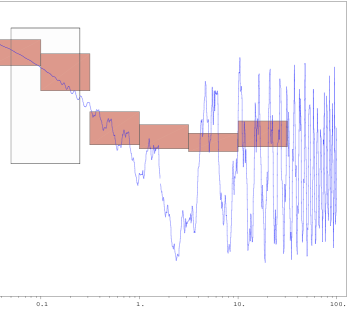
Figure 2: Taken from Fig. 5 of Ref. [8] to show the wiggly pattern in the $L/E$ dependence, with a moderate coupling to the infinite tower of KK neutrinos. The boxes are the Super-Kamiokande and K2K results.

In this case many KK modes are excited. The oscillation pattern gets very wiggly and very complicated, as illustrated in Fig. 2 from a numerical calculation taken from Ref. [8]. It seems unlikely that this is the situation phenomenologically unless we are so unlucky to have missed all these ‘irregular’ patterns so far.

4.4 Strong coupling

One might think that if intermediate coupling is difficult to analyse, strong coupling will be impossible. This turns out not to be the case because the widths of the eigenstates become so large that they overlap with one another to eliminate most of the wiggly and complicated structure seen in intermediate couplings. In fact, perhaps somewhat surprisingly, the problem becomes exactly soluble $\!{}^{{\bf?}}$ even for the DDG model.

To explain how that comes about let us first examine the eigenvalues in the strong coupling limit ($d\gg m_{i},1$). For any $d>0$, we see from Fig. 1 that $r(\lambda)$ is a decreasing function of $\lambda$, with poles at $m_{i}$, but $\tan(\pi\lambda)$ is an increasing function of $\lambda$, with poles at half integers. Consequently, there is one and only one solution of (6) in any interval bounded by a neighboring pair of poles. As $d$ is increased, the solution slides towards bigger magnitude of $\tan(\pi\lambda)$, i.e., $\lambda$ increases if $r(\lambda)>0$ and decreases if $r(\lambda)<0$. When $d\to\infty$, an eigenvalue must end up at the boundary of the interval, or at a zero of $r(\lambda)$. It is not difficult to show that the eigenvalues then consist of all half integers, plus the $f-1$ zeros of $r(\lambda)$. We denote the former by $\lambda^{\prime}_{n}=n+{1\over 2}\ (n\in{\bf Z})$, and the latter by $\lambda_{\ell}\ (2\leq\ell\leq f)$. $\lambda^{\prime}_{n}$ will be referred to as the regular eigenvalues, and $\lambda_{\ell}$ will be referred to as the isolated eigenvalues. Note that for large $d$, the brane and bulk neutrinos are quite thoroughly mixed up so we can no longer tell whether an eigenvector is more brane-like or more bulk-like. In particular, if we trace an isolated eigenvalue continuously back to $d=0$, depending on the precise values of $e_{i}$ and $m_{i}$, sometimes it ends up as a brane eigenvalue $m_{i}$, and sometimes it ends up as a bulk eigenvalue $n$.

Next let us look at $B^{2}(\lambda)$ and $U_{i\lambda}$. They behave differently for the two kinds of eigenvalues, because $\tan(\pi\lambda)$ is infinite for the regular eigenvalues and finite for the isolated eigenvalues. For this reason, it is more convenient to write (9) for the regular eigenvalues in the form $B^{2}(\lambda)=d^{2}s(\lambda)+1+d^{2}\tan^{2}(\pi\lambda)$, from which we see that $B^{2}(\lambda)=O(d^{2})$ and $U_{j\lambda}$ is finite in the large-$d$ limit. For regular eigenvalues, $r(\lambda)$ is non-zero, so we see from (9) that $B(\lambda)$ is of order $d^{4}$. This means that $U_{j\lambda}$ vanishes in the limit for every $\lambda$ of order unity. However, it does not mean that the sum in (2) over all regular eigenvalues is zero, because there is an infinite number of regular eigenvalues. In fact, for large $\lambda$ of order of $d^{2}$, we have $r(\lambda)\simeq 1/\lambda$ and $s(\lambda)\simeq 1/\lambda^{2}$, so $B^{2}(\lambda)\simeq 1+d^{2}(1+\pi^{2}d^{2})/\lambda^{2}\equiv 1+K^{2}/\lambda^{2}$ is finite for fixed $d^{2}/\lambda$ in the strong coupling limit. As a result, the sum in (2) over the regular eigenvalues can be replaced by the sum between $n=\pm N$ and $\pm\infty$, for any finite number $N$. We will choose $N$ so that $\lambda^{\prime}_{N}\gg 1,m_{i}$, then this sum can in turn be replaced by an integral, yielding

$${\cal A}^{reg}_{ij} = \sum_{n=-\infty}^{\infty}U^{*}_{i\lambda_{n}}U_{j\lambda_{n}}r^{-i\lambda_{n}^{2}\tau}$$ (14)

$$= e_{i}e_{j}\int_{-\infty}^{\infty}d\lambda{d^{2}e^{-i\lambda^{2}\tau}\over\lambda^{2}+K^{2}}$$

$$= e_{i}e_{j}g(K^{2}\tau),$$

where

$$g(x) \equiv {1\over\pi}\int_{-\infty}^{\infty}du{e^{-iu^{2}x}\over u^{2}+1}$$ (15)

begins at $g(0)=1$. Its absolute value decreases monotonically in $x$, approaching $g(x)\simeq(1-i)/\sqrt{2\pi x}$ for large $x$.

This leaves the sum over isolated eigenvalues. Since $U_{i\lambda}$ is finite for these eigenvalues, the transition in the strong coupling limit is amplitude

$${\cal A}_{ij}(\tau) = e_{i}e_{j}\Bigg{[}g(K^{2}\tau)+\sum_{\ell=2}^{f}{e^{-i\lambda_{\ell}^{2}\tau}\over s(\lambda_{\ell})(\lambda_{\ell}-m_{i})(\lambda_{\ell}-m_{j})}\Bigg{]}$$ (16)

$$\equiv V^{*}_{i1}V_{j1}g(K^{2}\tau)+\sum_{\ell=2}^{f}V^{*}_{i\ell}V_{j\ell}e^{-i\lambda_{\ell}^{2}\tau}$$

It can be verified that the $f\times f$ matrix $V$ is unitary (actually real orthogonal), so that ${\cal A}_{ij}(0)=\delta_{ij}$ as it should. If the function $g(K^{2}\tau)$ were replaced by $e^{-i\lambda_{1}^{2}\tau}$ (for some $\lambda_{1}$), then (16) would just be the usual transition amplitude of $f$ fermions, with a mixing matrix $V_{ij}$ and no bulk neutrino. In that case unitarity of $V$ guarantees the conservation of (brane) neutrino probability, namely, ${\cal P}_{j}(\tau)\equiv\sum_{i=1}^{f}{\cal P}_{ij}(\tau)=1$ for all $\tau$. With the presence of $g(K^{2}\tau)$ in (16), there is a leakage into the bulk so the total brane neutrino probability decreases with ‘time’, as in

$${\cal P}_{j}(\tau)=1-|e_{j}|^{2}\{1-|g(K^{2}\tau)|^{2}\}.$$ (17)

This reaches an asymptotic amount $1-|e_{j}|^{2}$ for large $\tau$. Since $\sum_{j}|e_{j}|^{2}=1$, the average leakage per brane channel is $1/f$.

5 Phenomenology

According to the Super-Kamiokande analysis of their data $\!{}^{{\bf?}}$, the mixing angle for atmospheric neutrino is large, and the mixing with sterile neutrino is small. Their data on solar neutrino favor the large angle MSW solution LMA, without much mixing with a sterile neutrino. However, this conclusion on solar neutrino depends somewhat how the data are analysed. The small angle (SMA) and the vacuum oscillation (VAC) solutions, with or without a large amount of sterile neutrino present, are not completely ruled out $\!{}^{{\bf?}}$, even with the recent charge current data from SNO $\!{}^{{\bf?}}$ taken into account.

There have been several attempts to understand the data from bulk neutrino models $\!{}^{{\bf?},{\bf?}}$. Unfortunately the data pose considerable difficulties on the simple DDG/ADDM model, which contains only one bulk neutrino and has no direct mixing between the active neutrinos. In the weak coupling limit when the mixing is small, there is no way this simple model can be applied to the atmospheric neutrino problem. Motivated by the 2+2 solution introduced to explain also the LSND data $\!{}^{{\bf?}}$, in which $(\nu_{\mu},\nu_{\tau})$ and $(\nu_{e},\nu_{s})$ form nearly degenerate doublets separated by about 1 eV, and the solar neutrino oscillates mostly to the sterile neutrino, attempts have been made to use the DDG/AGGM model to explain the solar neutrino problem. However, the 2+2 solution contains one sterile neutrino $\nu_{s}$, but the DDG/ADDM model contains an infinite tower of them. With more sterile neutrinos present the oscillation pattern becomes more complicated, and this can be utilized to cure the wrong energy dependence in the Super-K data caused by a single $\nu_{s}$. Two groups have succeeded in fitting the solar neutrino data, before the SNO data became available anyway, either with a $f=1$ DDG model $\!{}^{{\bf?}}$, or by introducing a mass for the bulk neutrino in the $f=1$ ADDM model $\!{}^{{\bf?}}$. To be able to explain also the atmospheric and perhaps the LSND data, one must modify the DDG/ADDM model, by introducing direct mixing between the active neutrinos, by introducing three bulk neutrinos, or by some other means.

One might think that the large mixing of atmospheric neutrino, and perhaps also of the solar neutrino, could possibly be explained by the DDG/ADDM model in the presence of a strong coupling. However, strong coupling also diverts a considerable amount of active neutrino flux into sterile neutrinos (the first term within the square brackets in (16)), which is forbidden by the data. Nevertheless, if the diversion comes mostly from an incoming $\nu_{\tau}$ beam, for which there is no data, it is conceivable that it might still work. In other words, we might attempt to make $e_{\tau}$ in (17) close to 1 and $e_{e},e_{\mu}$ small, in which case there is not much leakage of the solar and atmospheric neutrino fluxes into the sterile channels. Unfortunately this does not work for the $f=3$ DDG model, because with the vanishing of the first term of (16) for $\tau\gg 1/K^{2}$, there remains only $f-1=2$ terms in (16) and only one square-mass difference, impossible to explain both the atomospheric and the solar oscillations. Whether there is a way to make this work for $f\geq 4$ has not yet been analysed.

Figure 1: Graphical solutions of the characteristic equation (6). The left hand side of (6) is represented by the solid curve; the right hand side is represented by the dashed curves, with $(m_{1},m_{2},m_{3})=(-1.8,-0.2,0.3)$. The one with the short dash has the larger coupling constant $d$ than the one with the long dash. Note that the solution $\lambda$ moves up and right along the solid curve for increasing $d$ when the value on both sides of (6) is positive, and moves down and left along the solid curve when the value is negative.

References

- [1] T. Kaluza, Math. Phys. Kl (1921) 966; O. Klein, Phys. Z. 37 (1926) 895.
- [2] N. Arkani-Hamed, S. Dimopoulos, and G. Dvali, Phys. Lett. B429 (1998) 263; Phys. Rev. D59 (1999) 086004; I. Antoniadis, N. Arkani-Hamed, S. Dimopoulos, and G. Dvali, Phys. Lett. B436 (1998) 257; I. Antoniadis, Phys. Lett. B246 (1990) 317.
- [3] J. Polchinski, ‘String Theory’, Cambridge University Press, 1998.
- [4] J.C. Long, A.B. Churnside, and J.C. Price; C.D. Hoyle et. al., Phys. Rev. Lett. 86 (2001) 1418.
- [5] L. Randall and R. Sundrum, Phys. Rev. Lett. 83(1999) 3370, 4690; Y. Grossman and M. Neubert, Phys. Lett. B474 (2000) 361; S.J. Huber and Q. Shafi, hep-ph/0104293.
- [6] K.R. Dienes, E. Dudas, and T. Gherghetta, Nucl. Phys. B557 (1999) 25.
- [7] N. Arkani-Hamed, S. Dimopoulos, G. Dvali, and J. March-Russell, hep-ph/9811448.
- [8] N. Cosme, J.-M. Frere, Y. Gouverneur, F.-S. Ling, D. Monderen, V. Van Elewyck, Phys. Rev. D63 (2001) 113018.
- [9] C.S. Lam and J.N. Ng, hep-ph/0104129, to appear in Phys. Rev. D.
- [10] The Super-Kamiokande Collaboration, hep-ex/0009001, 0103032, 0103033.
- [11] V. Barger, D. Marfatia, and K. Whisnant, hep-ph/0106207; J.N. Bahcall, M.C. Gonzalez-Garcia, and C. Peña-Garay, hep-ph/0106258.
- [12] The SNO Collaboration, nucl-ex/0106015.
- [13] G. Dvali and A.Yu. Smirnov, Nucl. Phys. B563 (1999) 63-81; R.N. Mohapatra and A. Pérez-Lorenzana, Nucl. Phys. B576 (2000) 466, B596 (2001) 451; R. Barboero. Creminelli, and A. Strumia, Nucl. Phys. B585 (2000) 28; K.R. Dienes and I. Sarcevic, Phys. Lett. B500 (2001) 133.
- [14] C. Athanassopoulos et al., Phys. Rev. Lett. 77 (1996) 3082.
- [15] D.O. Caldwell, R.N. Mohapatra, and S. J. Yellin, Phys. Rev. Lett. 87 (2001) 041601, hep-ph/0101043, hep-ph/0102279.
- [16] A. Lukas, P. Ramond, A. Romanino, and G.G. Ross, Phys. Lett. B495 (2000) 136.