THEP 01/13
TTP01-19
hep-ph/0108197
August 2001

The Cross Section of $e^{+}e^{-}$ Annihilation into Hadrons of Order $\alpha_{s}^{4}n_{f}^{2}$
in Perturbative QCD

Abstract

We present the first genuine QCD five-loop calculation of the vacuum polarization functions: analytical terms of order $\alpha_{s}^{4}n_{f}^{2}$ to the absorptive parts of vector and scalar correlators. These corrections form an important gauge-invariant subset of the full ${\cal O}(\alpha_{s}^{4})$ correction to $e^{+}e^{-}$ annihilation into hadrons and the Higgs decay rate into hadrons respectively. They discriminate between different widely used estimates of the full result.

The value of the strong coupling $\alpha_{s}$ is one of the fundamental constants of Nature, comparable in its importance to the electromagnetic fine structure constant $\alpha_{\rm em}$ or the weak coupling $\alpha_{\rm weak}$, characterizing the coupling strength of the charged $W$ boson to lefthanded fermions. A precise measurement of $\alpha_{s}$ is important for the prediction of numerous observables in the framework of Quantum Chromodynamics (QCD). The comparison between the values determined with the methods of perturbative QCD (pQCD) at high energies and from lattice simulations respectively gives insight in to the quality of approximation methods and the validity of the overall framework. The combination of precise values of the three couplings $\alpha_{s}$, $\alpha_{\rm em}$ and $\alpha_{\rm weak}$ in the context of Grand Unified Theories leads, last but not least, to important information on the structure and the particle content of these theories beyond the Standard Model.

From the theoretical viewpoint the cross section for electron-positron annihilation into hadrons (or its variants like the $Z$-boson decay rate into hadrons or the semileptonic branching ratio of the $\tau$-lepton into hadrons) can be reliably predicted in pQCD and thus leads to one of the “gold-plated” $\alpha_{s}$ determinations.

Nontrivial QCD effects in these observables start at order $\alpha_{s}^{2}$ and their early evaluation CheKatTka79+NPB80 has laid the ground for the subsequent developments, both on the experimental and theoretical side (for a review see, e.g. ckk96 ). During the past years, in particular through the analysis of $Z$ decays at LEP and of $\tau$ decays, an enormous reduction of the experimental uncertainty (down to 3%) has been achieved with the perspective of a further reduction by a factor of four at a future linear collider TESLA .

Inclusion of the ${\cal O}(\alpha_{s}^{3})$ corrections GorKatLar91SurSam91 is thus mandatory already now. Quark mass effects as well as corrections specific to the axial current KniKue90b must be included for the case of $Z$-decays. The remaining theoretical uncertainty from uncalculated higher orders is at present comparable to the experimental one QCDreview . This has led to numerous estimates of the ${\cal O}(\alpha_{s}^{4})$ terms based on principles like that of “minimal sensitivity” (PMS), or of fastest apparent convergence (FAC) or by invoking the large $\beta_{0}$ limit (“naive nonabelization” (NNA)) etc. ste ; gru ; BG . In fact, already now the extraction of $\alpha_{s}$ from $\tau$-decays depends crucially on the corresponding estimates (see, e.g. QCDreview ).

The new calculational methods used in CheKatTka79+NPB80 , in particular recurrence relations based on the method of integration by parts me81b , had opened the door also to the four-loop calculation. Nevertheless, it took more than ten years of refinement of theoretical tools and development of the algebraic programs to move from the three to the four-loop calculation GorKatLar91SurSam91 .

It should be noted that much of this effort went into development of the algebraic program MINCER mincer2 written in FORM Ver91 , which implements the integration-by-parts algorithm to evaluate massless three loop propagators. An important part of the calculation, the generation of diagrams and their ultraviolet renormalization, was performed manually. In this context it is essential that one initially encounters the absorptive parts of four-loop amplitudes whose evaluation is reduced to that of three-loop propagators, employing the $R^{*}$ operation me84 . That latter step was also performed manually — an error-prone and time-consuming procedure difficult to implement in computer algebra, hence presenting a real obstacle for the ${\cal O}(\alpha_{s}^{4})$ calculation.

Recently the order ${\cal O}(\alpha_{s}^{3})$ result has been rederived in a general covariant gauge in a completely automatic way gvvq . This latter work was based on a general formula which explicitly expresses the result in terms of well-known renormalization constants and three-loop massless propagators, thus resolving the complicated combinatorics of ultraviolet and infrared subtractions. This formula is valid for any number of loops and is, therefore, an important ingredient of the present ${\cal O}(\alpha_{s}^{4})$ calculation.

The calculational effort for a full evaluation of $R(s)$ in ${\cal O}(\alpha_{s}^{4})$ is enormous and exceeds the presently available computer resources by perhaps two orders of magnitude. It is for this reason that we limit the present calculation to a gauge invariant subset, namely the terms of order $\alpha_{s}^{4}n_{f}^{2}$, where $n_{f}$ denotes the number of fermion flavours. The terms of order $\alpha_{s}^{4}n_{f}^{3}$ (and, in fact, all terms of order $\alpha_{s}(\alpha_{s}n_{f})^{n}$) have been obtained earlier by summing the renormalon chains VV:renormalons . These give interesting insight into the behavior of perturbation series in high orders and have been confirmed by the present work. However, they are numerically small and not directly sensitive to the nonabelian character of QCD, in contrast to the terms of order $\alpha_{s}^{4}n_{f}^{2}$.

The motivation of the present work is threefold. First: presenting the first ${\cal O}(\alpha_{s}^{4})$ results in pQCD demonstrates that the methods proposed in gvvq ; bai1 ; bai2 are indeed suited to obtain genuine QCD results in five loop approximation. Second: the results per se are an important ingredient of $R(s)$. And third: when comparing the exact $\alpha_{s}^{4}n_{f}^{2}$ results with the estimates based on various optimization procedures one obtains important insights into the quality of different approaches, confirming some and refuting others.

Below we will present the results for the vector correlator and the corresponding quantity $R(s)$ discussed above, and for the semileptonic branching ratio of the $\tau$ lepton. The same methods are applied for the scalar correlator. In this case the results are of relevance for the Higgs decays into quarks, for the QCD sum rule determinations of the strange quark mass and, last not least, they provide a second independent check of the “optimization procedures”.

Let us now briefly describe the methods used for the practical calculations. Using the techniques from gvvq and the known renormalization constants up to order $\alpha_{s}^{4}$ the four loop propagator type massless integrals remain to be evaluated. They were calculated following the method described in bai1 ; bai2 . It is based on the integration by part (IBP) technique me81b , however with important modifications. The integral is to be reduced to a sum of irreducible (“master”) integrals with coefficients that are known to be rational functions of the space-time dimension $D$. However, in contrast to the original approach, where these coefficients were calculated by a recursive procedure, they are in the current approach obtained from an auxiliary integral representationbai1 .

For three-loop vacuum integrals these representations can be solved explicitly in terms of Pochhammers symbols bai1 . The structure of four-loop propagators is much more involved and an explicit solution is not available. In the present case the following method is used: for massless propagators the coefficients of the master integrals should be rational functions of space-time dimension $D$ only. Their integral representation is expanded in the limit $1/D\rightarrow 0$. Calculating sufficiently many terms in this expansion, the original $D$-dependence can be reconstructed. This approach is essentially different from $1/D$ expansion for the very Feynman integrals, recently proposed in Ref. Tar . In our case only the coefficients of the master integrals (rational functions in $D$!) are expanded and the original integral can be reconstructed exactly.

In practice we proceed as follows: First, the set of irreducible integrals involved in the problem was constructed, using the criterion irreducibility of Feynman integrals bai2 . Second, the coefficients multiplying these master integrals were calculated in the $1/D\rightarrow 0$ expansion. This part was performed using the parallel version of FORM Fliegner:2000uy running on an 8-alpha-processor-SMP-machine with disk space of 350 GB. The calculations took approximately 500 hours in total. (The time includes $\approx$ 300 hours spent on the single diagram presented on Fig. 1a, which demonstrates that trivial parallelization by assigning different diagrams to different machines is not feasible.) Third, the exact answer was reconstructed from results of these expansions. Extensive tests were performed. Dealing with four-loop integrals, the result cannot have the singularities stronger then $1/(D-4)^{4}$ in $D\rightarrow 4$ limit. The contributions corresponding to individual master integrals have poles up to $1/(D-4)^{6}$ which cancel in the final expression. Furthermore, singular parts of all diagrams were checked by MINCER. Previously obtained four-loop results were successfully reproduced.

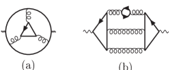
Figure 1: (a) Diagram whose calculation took $\approx$ 300 hours. (b) Diagram contributing to the QED $\beta$-function in ${\cal O}(\alpha_{\rm em}^{6}n_{f}^{3})$.

It is convenient to define “Adler functions” as

$$D(Q^{2})=\int_{0}^{\infty}\frac{Q^{2}\ R(s)ds}{(s+Q^{2})^{2}}{},\ \ \widetilde{D}(Q^{2})=\int_{0}^{\infty}\frac{Q^{2}\ \widetilde{R}(s)ds}{(s+Q^{2})^{2}}{}\ .$$

Here, $R(s)=1+\alpha_{s}/\pi+\dots$ is the famous $R$-ratio in the massless limit (we suppress the trivial factor $\sum_{f}Q^{2}_{f}$ throughout) and $\widetilde{R}(s)=1+\frac{17}{3}\alpha_{s}/\pi+\dots$ is properly normalized imaginary part of the scalar polarization function. Our results for $D,\widetilde{D},R$ and , $\tilde{R}$ are presented below. Let us define ($a_{s}\equiv\alpha_{s}/\pi$)

$$D(Q^{2}) = 1+\sum_{i=1}^{\infty}d_{i}\ a_{s}^{i}(Q^{2}),\ \ R(s)=1+\sum_{i=1}^{\infty}r_{i}\ a_{s}^{i}(s)\ ,$$

$$\widetilde{D}(Q^{2}) = 1+\sum_{i=1}^{\infty}\ \widetilde{d}_{i}a_{s}^{i}(Q),\ \ \tilde{R}(s)=1+\sum_{i=1}^{\infty}\ \tilde{r}_{i}a_{s}^{i}(s){}\ ,$$

where we have set the normalization scale $\mu^{2}=Q^{2}$ or to $\mu^{2}=s$ for the euclidian and minkowskian functions respectively. The results for generic values of $\mu$ can be easily recovered with the standard RG techniques. Since the functions $D$ and $\tilde{D}$ are known to order $\alpha_{s}^{3}$ from Refs. GorKatLar91SurSam91 ; gvvq ; gssq we cite below only the ${\cal O}(\alpha_{s}^{4})$ results (dots stand for still unknown terms of order $\alpha_{s}^{4}n_{f}$ and $\alpha_{s}^{4}n_{f}^{0}$).

$$d_{4}=\,C_{F}\,n_{f}^{3}\left[-\frac{6131}{7776}+\frac{203}{432}\,\zeta_{3}+\frac{5}{24}\,\zeta_{5}\right]$$ (1)

$${+} \,C_{F}\,C_{A}\,n_{f}^{2}\left[\frac{340843}{20736}-\frac{10453}{1152}\,\zeta_{3}-\frac{1}{8}\,\zeta_{3}^{2}-\frac{85}{18}\,\zeta_{5}\right]$$

$${+} C_{F}^{2}\,n_{f}^{2}\left[\frac{5713}{6912}-\frac{581}{96}\,\zeta_{3}+\frac{3}{4}\,\zeta_{3}^{2}+\frac{125}{24}\,\zeta_{5}\right]+\dots$$

$$\widetilde{d}_{4}=\,C_{F}\,n_{f}^{3}\left[-\frac{520771}{746496}+\frac{65}{576}\,\zeta_{3}+\frac{1}{192}\,\zeta_{4}+\frac{5}{24}\,\zeta_{5}\right]$$ (2)

$${+} C_{F}^{2}\,n_{f}^{2}\left[\frac{7009861}{497664}-\frac{4073}{384}\,\zeta_{3}\right.$$

$$\hskip 65.44142pt\left.+\frac{3}{4}\,\zeta_{3}^{2}-\frac{15}{128}\,\zeta_{4}+\frac{89}{24}\,\zeta_{5}\right]$$

$${+} \,C_{F}\,C_{A}\,n_{f}^{2}\left[\frac{18248293}{995328}-\frac{1243}{576}\,\zeta_{3}\right.$$

$$\hskip 48.36958pt\left.-\frac{1}{8}\,\zeta_{3}^{2}+\frac{15}{128}\,\zeta_{4}-\frac{2621}{576}\,\zeta_{5}\right]{}+\dots,$$

$${}r_{4} = \,n_{f}^{3}\left[-\frac{6131}{5832}+\frac{11}{432}\pi^{2}+\frac{203}{324}\,\zeta_{3}-\frac{1}{54}\pi^{2}\,\zeta_{3}+\frac{5}{18}\,\zeta_{5}\right]$$

$${+} \,n_{f}^{2}\left[\frac{1045381}{15552}-\frac{593}{432}\pi^{2}-\frac{40655}{864}\,\zeta_{3}\right.$$

$$\hskip 45.52458pt+\ \left.\frac{11}{12}\pi^{2}\,\zeta_{3}+\frac{5}{6}\,\zeta_{3}^{2}-\frac{260}{27}\,\zeta_{5}\right]+\dots{},$$

$$\widetilde{r}_{4} = n_{f}^{3}\left[-\frac{520771}{559872}+\frac{275}{3888}\pi^{2}-\frac{1}{2160}\pi^{4}\right.$$

$$\hskip 22.76228pt+\left.\frac{65}{432}\,\zeta_{3}-\frac{1}{54}\pi^{2}\,\zeta_{3}+\frac{1}{144}\,\zeta_{4}+\frac{5}{18}\,\zeta_{5}\right]$$

$${+} \,n_{f}^{2}\left[\frac{220313525}{2239488}-\frac{197119}{31104}\pi^{2}-\frac{11875}{432}\,\zeta_{3}+\frac{5}{6}\,\zeta_{3}^{2}\right.$$

$${+} \left.\frac{143}{4320}\pi^{4}+\frac{259}{216}\pi^{2}\,\zeta_{3}+\frac{25}{96}\,\zeta_{4}-\frac{5015}{432}\,\zeta_{5}\right]+\dots$$

In (1) and (2) we have distinguished between contributions proportional to different color factors, while for ( THEP 01/13 TTP01-19 hep-ph/0108197 August 2001 The Cross Section of $e^{+}e^{-}$ Annihilation into Hadrons of Order $\alpha_{s}^{4}n_{f}^{2}$ in Perturbative QCD) and ( THEP 01/13 TTP01-19 hep-ph/0108197 August 2001 The Cross Section of $e^{+}e^{-}$ Annihilation into Hadrons of Order $\alpha_{s}^{4}n_{f}^{2}$ in Perturbative QCD) their SU(3) values $C_{F}=4/3$, $C_{A}=3$ have been specified. In ( THEP 01/13 TTP01-19 hep-ph/0108197 August 2001 The Cross Section of $e^{+}e^{-}$ Annihilation into Hadrons of Order $\alpha_{s}^{4}n_{f}^{2}$ in Perturbative QCD) and ( THEP 01/13 TTP01-19 hep-ph/0108197 August 2001 The Cross Section of $e^{+}e^{-}$ Annihilation into Hadrons of Order $\alpha_{s}^{4}n_{f}^{2}$ in Perturbative QCD) we differentiate between $\zeta_{4}$-terms and $\pi^{4}$-ones generated by the analytic continuation from spacelike to timelike regions. At last, numerically $R$ and $\widetilde{R}$ read

$$R(s)=1+a_{s}+a_{s}^{2}\left(1.986-0.1153\ n_{f}\right)$$

$$+ a_{s}^{3}\left(-6.6369-1.2001\ n_{f}-0.00518\ n_{f}^{2}\right)$$

$$+ a_{s}^{4}\left(0.02152\ n_{f}^{3}-0.7974\ n_{f}^{2}+\ n_{f}\ r_{(4,1)}+r_{(4,0)}\right){},$$

$$\widetilde{R}(s)=1+5.6667\ a_{s}+a_{s}^{2}\left(35.940-1.3586\ n_{f}\right)$$

$$+ a_{s}^{3}\left(164.1392-25.7712\ n_{f}+0.2590\ n_{f}^{2}\right)$$

$$+ a_{s}^{4}\left(-0.02046\ n_{f}^{3}+9.6848\ n_{f}^{2}+\ n_{f}\ \tilde{r}_{(4,1)}+\tilde{r}_{(4,0)}\right){}.$$

The result is easily applied to the semileptonic $\tau$ decay rate. Numerically one finds for the QCD corrections to the parton result in the massless limit

$$R^{\tau}=1 + a_{s}+5.2023\ a_{s}^{2}+26.3659\ a_{s}^{3}$$ (7)

$$+ a_{s}^{4}\ (6.1827n_{f}^{2}-0.06368n_{f}^{3}){},$$

where we have set $\mu=M_{\tau}$ and $n_{f}=3$ everywhere except for the ${\cal O}(a_{s}^{4})$ term.

Another application of our results is the QED $\beta$-function. At four-loops it is known from GorKatLarSur91 . At five-loops the only available information is the leading at large $n_{f}$ term of order $\alpha^{6}n_{f}^{4}$ QED-beta:renorm.chain . For QED with $n_{f}$ electron flavours we find a partial result for the term of order ${\cal O}(\alpha^{6}n_{f}^{3})$, viz.

$$\beta_{QED}(\alpha)=\,n_{f}\left[\frac{4\ A^{2}}{3}\right]{+}4\,n_{f}A^{3}-A^{4}\left[2\,n_{f}+\frac{44}{9}\,n_{f}^{2}\right]$$ (8)

$${+} A^{5}\left[-46\,n_{f}+\frac{760}{27}\,n_{f}^{2}-\frac{832}{9}\,\zeta_{3}\,n_{f}^{2}-\frac{1232}{243}\,n_{f}^{3}\right]$$

$${+} A^{6}\left[\frac{9922}{81}\,n_{f}^{3}-\frac{7616}{27}\,\zeta_{3}\,n_{f}^{3}+\frac{352}{3}\,\zeta_{4}\,n_{f}^{3}\right.$$

$$\hskip 56.9055pt\left.\ +\ \frac{856}{243}\,n_{f}^{4}+\frac{128}{27}\,\zeta_{3}\,n_{f}^{4}\right]{},$$

where $A=\alpha/(4\pi),\alpha=e^{2}/(4\pi)$ and $e$ is the electron electric charge.

Table 1: Comparison of the results obtained in this paper with estimates based of FAC, PMS, NNA and two types of Padé approximation methods.

$r_{(4,2)}$	$\tilde{r}_{(4,2)}$
-0.797	9.685	exact
-1.06	—	KS (PMS), Samuel:1995jc (PAM)
—	7.71	CheKniSir97 (PMS, FAC)
0.74	25.2	HPade (APAM)
—	1.00	Broadhurst:2001yc (NNA)

In Table I our results are compared with predictions obtained with the help of various optimization procedures. To get these numbers we have taken the predictions of KS ; Samuel:1995jc ; CheKniSir97 ; HPade ; Broadhurst:2001yc (where available) for $n_{f}=3,4,5$, have subtracted the ${\cal O}(\alpha_{s}^{4}n_{f}^{3})$ contribution and fitted the result against the quadratic polynomial in $n_{f}$. For both correlators the predictions based on the Principle of Minimal Sensitivity (PMS) or on fastest apparent convergence (FAC) or, at last, on the Padé Approximation Method (PAM) are in quite good agreement to the exact results. On the other hand, Asymptotic Padé-Approximant Method (APAM) as well as Naive NonAbelization (NNA) fail to predict even the rough size of the $\alpha_{s}^{4}n_{f}^{2}$ coefficients. All in all one may conclude that there is a good chance that

• the often used prediction by Kataev and Starshenko for the complete ${\cal O}(\alpha_{s}^{4})$ contribution to the vector correlator will be close to reality;

• the relatively worser apparent convergence of the perturbative series for the scalar correlator as revealed by the calculation of Ref. gssq will persist in higher orders in agreement with FAC/PMS estimations of Ref. CheKniSir97 .

Finally, we note that the present calculation does not include all possible topological types of diagrams appearing in order $\alpha_{s}^{4}$. Nevertheless, our experience shows that these new topologies can be solved in the same way, given sufficient computer resources. Work in this direction is in progress.