Bilepton gauge boson contribution to the static electromagnetic properties of the W boson in the minimal 331 model

Abstract

We present a complete calculation of the singly and doubly charged gauge bosons (bileptons) contribution to the static properties of the $W$ boson in the framework of the minimal 331 model, which accommodates the bileptons in an $\mathrm{SU_{L}(2)}$ doublet. A nonlinear $R_{\xi}$ gauge is used and a slightly modified version of the Passarino-Veltman reduction scheme is employed as in this case the Gram determinant vanishes. It is found that the bilepton contribution is of the same order of magnitude as those arising from other weakly coupled renormalizable theories, like the two-Higgs doublet model and supersymmetry. The heavy mass limit is explored and the nontrivial decoupling properties of bileptons are discussed. Although there is a close resemblance with the contribution of an $\mathrm{SU_{L}(2)}$ fermion doublet, in the case of the bilepton doublet the decoupling theorem does remain valid. As a by-product, we present a detailed study of the trilinear and the quartic vertices involving the bileptons and the standard model gauge bosons.

I Introduction

One of the main goals of the next generation of high energy colliders will be to probe the Yang-Mills sector of the standard model (SM). In order to measure the $WW\gamma$ and $WWZ$ gauge couplings, the most promising production modes are $WZ$ and $W\gamma$ at hadron colliders and $WW$ at $e^{+}e^{-}$ linear colliders. With a high experimental accuracy, these modes would allow to test these couplings beyond tree level, which is essential for studying the gauge cancellations that arise at one-loop level. The study of these couplings also offers a unique opportunity to find any evidence of heavy physics lying beyond the Fermi scale. In particular, the on-shell electromagnetic properties of the $W$ boson have been the subject of constant interest since they can be sensitive to new physics effects. These quantities are the anomalous (one-loop) magnetic dipole moment and the electric quadrupole moment, which are characterized by two parameters denoted by $\Delta\kappa$ and $\Delta Q$. They appear as coefficients of Lorentz structures of canonical dimension 4 and 6, respectively. In the SM, both $\Delta\kappa$ and $\Delta Q$ vanish at tree level. This means that these parameters can only receive contributions at one-loop level in any renormalizable theory and may be sensitive to new physics effects, which might compete with the SM contribution. We will see below that a high precision measurement of $\Delta Q$ can only be useful to looking for physics effects not very far beyond the Fermi scale. In contrast, $\Delta\kappa$ may be sensitive to heavy physics effects. Within the SM, the one-loop contributions to $\Delta Q$ and $\Delta\kappa$ from the gauge bosons, the Higgs scalar and massless fermions were studied in [1], whereas the top quark effects were analyzed later [2]. The sensitivity of these quantities to new physics effects has also been studied within some specific models, like the two-Higgs doublet model [3] and supersymmetric theories [4]. Further studies were also done within models with an extra ${Z^{\prime}}$ boson [5], composite particles [6], and an extra $W$ boson [7]. Both $\Delta Q$ and $\Delta\kappa$ have also been parametrized in a model independent way by using an effective Lagrangian approach, and the phenomenological consequences have been extensively studied both at hadronic and leptonic colliders [8].

In this work we are interested in studying the on-shell $WW\gamma$ vertex in the framework of the minimal $331$ model, which is based on the simplest nonabelian gauge-group extension of the SM, namely $\mathrm{SU_{c}(3)}\times\mathrm{SU_{L}(3)}\times\mathrm{U_{X}(1)}$ [9]. In particular, we will concentrate on the contributions coming from a pair of singly and doubly charged gauge bosons predicted by this model. These particles are called bileptons because they have two units of lepton number. The 331 model has attracted considerable attention recently [10] since it requires that the number of fermion families be a multiple of the quark color number in order to cancel anomalies, which offers a possible solution to the flavor problem. Another important feature of this model is that the $\mathrm{\mathrm{SU_{L}(2)}}$ group is totally embedded in $\mathrm{SU_{L}(3)}$. As a consequence, after the first stage of spontaneous symmetry breaking (SSB), when $\mathrm{SU_{L}(3)}\times\mathrm{U_{X}(1)}$ is broken down to $\mathrm{SU_{L}(2)}\times\mathrm{U_{Y}(1)}$, there emerge a pair of massive bileptons in a doublet of the electroweak group, giving rise to very interesting couplings with the SM gauge bosons. In particular, these couplings do not involve any mixing angle, as occurs in other SM extensions, and are similar both in strength and Lorentz structure to those couplings existing between the SM gauge bosons.

Besides their nontrivial transformation properties under the electroweak gauge group, the bileptons get a mass splitting at the Fermi scale due to the presence of some terms that violate the custodial $\mathrm{SU_{c}(2)}$ symmetry. It is well known, from the analysis of fermion or scalar doublets, that these peculiarities might give rise to nondecoupling effects in low-energy processes. For this reason, it is important to investigate the respective contribution to $\Delta\kappa$ and $\Delta Q$ on the basis of the decoupling theorem [11]. It is a known fact that a heavy particle might be detected through its virtual effects on low-energy physics if it evades the decoupling theorem [12]. This interesting phenomenon can occur only in theories with SSB, where some particles can have a mass heavier than the vacuum expectation value (VEV) scale due to a large coupling constant. In such a situation, the suppression factor arising from the propagator of the heavy particle is compensated by a mass factor appearing in the numerator, which in turn is determined by a large coupling constant. In contrast, a particle decouples in the heavy mass limit if its mass is induced by a gauge singlet bare parameter (usually an unfixed VEV) since dynamics compensatory effects are not present in this case. In this paper we will show that bileptons obey the decoupling theorem and, as a consequence, their contribution to both $\Delta\kappa$ and $\Delta Q$ vanishes in the heavy mass limit. This behavior is a result of the fact that a large mass implies a large parameter not fixed by experiment, namely a VEV larger than the electroweak scale. It is interesting to note that this case is similar to that studied in Ref. [13], in which an extra scalar doublet that does not develop a VEV was considered. On the other hand, the decoupling nature of $\Delta Q$ is not surprising, even if it receives contributions from a particle that violates the decoupling theorem. It turns out that this quantity is insensitive to a large physical scale [14]. This result is a consequence of the fact that $\Delta Q$ is parametrized by a dimension-6 Lorentz structure which is naturally suppressed by inverse powers of the mass of the heavy particle circulating in the loop, as was explicitly verified for the contribution of an extra fermion generation and technihadrons [14]. We will return to this point later in the context of the bilepton contribution.

In contrast to other extensions of the SM, in the $331$ model the mass of the extra gauge bosons is bounded from above as a consequence of matching the gauge coupling constants at the Fermi scale [15]. Therefore this model would be either confirmed or ruled out at the future high-energy colliders. Current bounds establish that bilepton masses may take values ranging from a few hundred of GeVs to about 1 TeV. This is an important reason to investigate the effect of these particles on the $WW\gamma$ vertex. We will show below that the respective contributions to $\Delta\kappa$ and $\Delta Q$ are comparable to those induced by other weakly coupled renormalizable theories.

Another point worth to mention concerns the approach we took to perform our calculation. In the first place, we found convenient to use a nonlinear $R_{\xi}$ gauge rather than the unitary gauge. For this aim we introduced a gauge-fixing term covariant under the $\mathrm{U_{e}(1)}$ gauge group, from which the necessary Feynman rules were derived. This gauge-fixing procedure allowed us to remove the mixed $YG_{Y}\gamma$ vertices. As for the evaluation of the tensorial integrals, it has been customary to use the Feynman parameters technique for evaluating the static properties of elementary particles. It turns out that, in this case, the Passarino-Veltman reduction method [16] breaks down since the Gram determinant of the kinematic matrix vanishes [17]. However, we will show below that, even in this case, the last method can be used after introducing some slight modifications.

The rest of the paper is organized as follows. In Sec. II we give a description of the minimal $331$ model. Particular emphasis is given to the Yang-Mills sector. In Sec. III we present the calculation of the static properties of the $W$ boson. Sec. IV is devoted to discuss our results, and the conclusions are presented in Sec. V. Finally, explicit expressions for both the trilinear and quartic vertices involving bilepton gauge bosons are presented in the Appendices, together with the respective Feynman rules.

II Review of the minimal $331$ model

To begin with, we present a short description of the fermionic sector of the minimal $331$ model. We will turn next to discuss in detail the gauge sector. In particular, we will focus on the mass spectrum and the coupling structure of the Yang-Mills sector. Hereafter, we will follow closely the notation and conventions of Ref. [18]. The simplest anomaly-free fermionic content of the 331 model accommodates the leptons as antitriplets of $\mathrm{SU_{L}(3)}$:

$$\ell^{i}_{L}=\left(\begin{array}[]{c}e^{i}_{L}\\ \nu^{i}_{L}\\ e^{c\,i}\end{array}\right):(1,3^{*},0),$$ (1)

where $i=1,2,3$ is the generation index. The quark sector includes three new exotic quarks. Two quark generations are given the same representation, and the third one (no matter what) is treated differently. It has been customary to represent the first two quark families as triplets and the third one as antitriplet [9]:

$$q_{L}^{i}=\left(\begin{array}[]{c}u^{i}_{L}\\ d^{i}_{L}\\ D^{i}_{L}\end{array}\right):~{}(3,3,-1/3),$$ (2)

$$u^{i}_{R}:~{}(3,1,-2/3);\quad d^{i}_{R}:~{}(3,1,+1/3);\quad D^{i}_{R}:~{}(3,1,+4/3);\qquad(i=1,2),$$ (3)

$$q^{3}_{L}=\left(\begin{array}[]{c}u^{3}_{L}\\ d^{3}_{L}\\ T^{3}_{L}\end{array}\right):~{}(3,3^{*},2/3),$$ (4)

$$u^{3}_{R}:~{}(3,1,+1/3);\quad d^{3}_{R}:~{}(3,1,-2/3);\quad T^{3}_{R}:~{}(3,1,-5/3).$$ (5)

In order to accomplish the gauge hierarchy and the fermion masses, a Higgs sector composed of several $\mathrm{SU_{L}(3)}$ multiplets is required: to break $\mathrm{SU_{L}(3)}\times\mathrm{U_{X}(1)}$ down to $\mathrm{SU_{L}(2)}\times\mathrm{U_{Y}(1)}$ only one $\mathrm{SU_{L}(3)}$ scalar triplet is necessary; the next stage of SSB, $\mathrm{SU_{L}(2)}\times\mathrm{U_{Y}(1)}\to\mathrm{U_{e}(1)}$, requires two scalar $\mathrm{SU_{L}(3)}$ triplets and one sextet. The minimal Higgs sector has the following quantum numbers

$$\phi_{Y}=\left(\begin{array}[]{c}\Phi_{Y}\\ \phi^{0}\end{array}\right):\quad(1,3,1);\quad\phi_{1}=\left(\begin{array}[]{c}\Phi_{1}\\ \delta^{-}\end{array}\right):\quad(1,3,0);\quad\phi_{2}=\left(\begin{array}[]{c}\widetilde{\Phi}_{2}\\ \rho^{--}\end{array}\right):\ \ \ (1,3,-1),$$ (6)

$$H=\left(\begin{array}[]{ccc}T&\widetilde{\Phi}_{3}/\sqrt{2}\\ \widetilde{\Phi}^{T}_{3}/\sqrt{2}&\eta^{--}\end{array}\right):\ \ \ (1,6,0),$$ (7)

where $T$ is a $2\times 2$ matrix given by

$$T=\left(\begin{array}[]{ccc}T^{++}&T^{+}/\sqrt{2}\\ T^{+}/\sqrt{2}&T^{0}\end{array}\right),$$ (8)

Both $\Phi_{Y}$ and $\Phi_{i}$ ($i=1,\,2,\,3$ and $\widetilde{\Phi}_{i}=i\,\tau^{2}\,\Phi^{*}_{i}$) are two-component complex quantities. We will see below that after the first stage of SSB all these quantities constitute a specific representation of the electroweak group. When $\phi_{Y}$ develops a VEV, $\mathrm{SU_{L}(3)}\times\mathrm{U_{X}(1)}$ breaks down to $\mathrm{SU_{L}(2)}\times\mathrm{U_{Y}(1)}$ and the exotic quarks and the new gauge bosons acquire masses. The remaining multiplets endow the SM particles with mass.

The covariant derivative in the fundamental representation of $\mathrm{SU_{L}(3)}\times\mathrm{U_{X}(1)}$ can be written as

$${D}_{\mu}=\partial_{\mu}-i\,g\,\frac{\lambda^{a}}{2}\,W^{a}_{\mu}-i\,g_{X}X\,\frac{\lambda^{9}}{2}\,X_{\mu},\qquad(a=1\ldots 8),$$ (9)

with $\lambda^{a}$ the Gell-man matrices and $\lambda^{9}=\sqrt{2/3}\;{\mathrm{d}iag(1,1,1)}$. The generators are normalized according to $\mathrm{Tr}\,\lambda^{a}\lambda^{b}=2\,\delta^{ab}$, which means that $\mathrm{Tr}\,\lambda^{9}\lambda^{9}=2$. The first stage of SSB is accomplished by the VEV of $\phi_{Y}$, $\phi^{\dagger}_{Y0}=(0,0,u/\sqrt{2})$, according to the following scheme: six generators are broken, namely $\lambda^{b}\phi_{Y0}\neq 0$ ($b=4\ldots 9$), whereas the remaining ones leave invariant the vacuum, namely $\lambda^{a}\phi_{Y0}=0$ ($a=1,\,2,\,3$). Notice that $\sqrt{3}\,(\lambda^{8}+\sqrt{2}X\lambda^{9})\phi_{Y0}=0$, so the hypercharge can be identified with a linear combination of broken generators as follows $Y=\sqrt{3}\,(\lambda^{8}+\sqrt{2}X\lambda^{9})$. At this stage of SSB, there appears one pair of singly and doubly charged bileptons, which are defined by

$$Y^{++}_{\mu}=\frac{1}{\sqrt{2}}\left(W^{4}_{\mu}-iW^{5}_{\mu}\right),\qquad Y^{+}_{\mu}=\frac{1}{\sqrt{2}}\left(W^{6}_{\mu}-iW^{7}_{\mu}\right),$$ (10)

and get a mass given by

$$M_{Y}={M_{Y^{++}}}={M_{Y^{+}}}=\frac{g\,u}{2}.$$ (11)

According to the quantum number assignment, the bilepton gauge bosons fill out one doublet of $\mathrm{SU_{L}(2)}\times\mathrm{U_{Y}(1)}$ with hypercharge $3$:

$$Y_{\mu}=\left(\begin{array}[]{c}Y^{++}_{\mu}\\ Y^{+}_{\mu}\end{array}\right).$$ (12)

The gauge fields $W^{8}_{\mu}$ and $X_{\mu}$ mix to produce a massive field, ${Z^{\prime}}_{\mu}$, and a massless gauge boson, $B_{\mu}$. The latter is associated with the $\mathrm{U_{Y}(1)}$ group. These fields are given by

$${Z^{\prime}}_{\mu} =c_{\theta}\,W^{8}_{\mu}-s_{\theta}\,X_{\mu},$$ (13)

$$B_{\mu} =s_{\theta}W^{8}_{\mu}+c_{\theta}X_{\mu},$$ (14)

$$M^{2}_{{Z^{\prime}}} =\frac{1}{6}\left(2\,g^{2}+g^{2}_{X}\right)u^{2},$$ (15)

$$M_{B} =0,$$ (16)

where $s_{\theta}=\sin\theta,c_{\theta}=\cos\theta$ and $\tan\theta=g_{X}/(\sqrt{2}\,g)$. The coupling constant associated with the hypercharge group is given by $g^{\prime}=g\,s_{\theta}/\sqrt{3}$. The remaining fields associated with the unbroken generators of $\mathrm{SU_{L}(3)}$ are the gauge bosons of the $\mathrm{\mathrm{SU_{L}(2)}}$ group, which will be denoted as $W^{i}_{\mu}$ ($i=1,2,3$).

In the Higgs sector, $\Phi_{Y}$ and $\Phi_{i}$ ($i=1,2$) are $\mathrm{\mathrm{SU_{L}(2)}}$ doublets with hypercharge $3$ and $1$, respectively. It can be shown that the two components of $\Phi_{Y}$ represent the pseudo-Goldstone bosons associated with the bilepton fields, while the real and imaginary part of $\phi^{0}$ correspond to a physical Higgs boson and the pseudo-Goldstone boson associated with the ${Z^{\prime}}$ field, respectively. The third components of $\phi_{1}$ and $\phi_{2}$, $\delta^{-}$ and $\rho^{--}$, are singlets of $\mathrm{\mathrm{SU_{L}(2)}}$ with hypercharge $-2$ and $-4$, respectively. The sextet $H$ is composed of the following structures: a doublet $\Phi_{3}$ with $Y=+1$, a triplet $T$ with $Y=+2$, and a singlet $\eta^{--}$ with $Y=+4$. As for the fermionic sector, in addition to the SM content of leptons and quarks, there appear three exotic quarks as singlets of $\mathrm{\mathrm{SU_{L}(2)}}$. Among these exotic quarks, two of them have electric charge $-4/3$, while the third one has electric charge $5/3$.

In summary, after the first stage of SSB we end up with the $\mathrm{SU_{c}(3)}\times\mathrm{SU_{L}(2)}\times\mathrm{U_{Y}(1)}$   gauge group and the SM content of leptons and quarks, plus three doublets and one triplet of scalar fields, one bilepton doublet, one neutral gauge boson (${Z^{\prime}}$), and several singlets of scalar and quark fields. The presence of a bilepton doublet is a remarkable feature of this class of models and may give rise to some interesting phenomenological consequences. The main aim of this work is to explore the effects of these exotic particles on the static electromagnetic properties of the $W$ gauge boson. The respective contributions to the $WW\gamma$ vertex are dictated entirely by the Yang-Mills sector of the model. It is interesting to note that the exotic quarks do not contribute to the $WW\gamma$ vertex since they are $\mathrm{\mathrm{SU_{L}(2)}}$ singlets and thus do not interact with the $W$ boson. Moreover, we will not consider the contributions from charged scalar Higgs boson as such kind of contributions have been studied widely within the two Higgs doublet model [3]. Therefore, our main concern lies on the structure of the Yang-Mills sector associated with the $\mathrm{SU_{L}(3)}\times\mathrm{U_{X}(1)}$ group. The analysis of the Higgs kinetic-energy terms is also required since this sector is responsible for the splitting between the bilepton masses. As it will be discussed below, such a splitting is a consequence of the violation of the custodial $\mathrm{SU_{c}(2)}$ symmetry. In addition, this sector requires some manipulation as we found convenient to use a renormalizable $R_{\xi}$ gauge for our calculation.

The full Yang-Mills Lagrangian is composed of the following three $\mathrm{SU_{L}(2)}\times\mathrm{U_{Y}(1)}$ invariant pieces

$${\cal L}_{\mathrm{YM}} =-\frac{1}{4}W^{a}_{\mu\nu}W^{\mu\nu}_{a}-\frac{1}{4}X_{\mu\nu}X^{\mu\nu},$$ (17)

$$={\cal L}_{\mathrm{SM}}+{\cal L}_{{\mathrm{SMNP}}}+{\cal L}_{{\mathrm{NP}}},$$ (18)

where ${\cal L}_{\mathrm{SM}}$ is the SM Yang-Mills Lagrangian given by

$${\cal L}_{\mathrm{SM}}=-\frac{1}{4}W^{i}_{\mu\nu}W^{\mu\nu}_{i}-\frac{1}{4}B_{\mu\nu}B^{\mu\nu}.$$ (19)

${\cal L}_{{\mathrm{SMNP}}}$, which comprises the interactions between the SM gauge bosons and the new ones, can be written as

$${\cal L}_{{\mathrm{SMNP}}}= -\frac{1}{2}\left(D_{\mu}Y_{\nu}-D_{\nu}Y_{\mu}\right)^{\dagger}\left(D^{\mu}Y^{\nu}-D^{\nu}Y^{\mu}\right)-Y^{{\dagger}\mu}\left(i\,g\,{\bf W}_{\mu\nu}+i\,g^{\prime}\,{\bf B}_{\mu\nu}\right)Y^{\nu}$$ (20)

$$-\frac{i\,\sqrt{3}\,g\,c_{\theta}}{2}{Z^{\prime}}_{\mu}\left[Y^{\dagger}_{\nu}\left(D^{\mu}Y^{\nu}-D^{\nu}Y^{\mu}\right)-\left(D^{\mu}Y^{\nu}-D^{\nu}Y^{\mu}\right)^{\dagger}Y_{\nu}\right]$$ (21)

where we have introduced the definitions ${\bf W}_{\mu\nu}=\tau^{i}\,W^{i}_{\mu\nu}/2$ and ${\bf B}_{\mu\nu}=Y\,B_{\mu\nu}$/2. In addition $D_{\mu}=\partial_{\mu}-ig{\bf W}_{\mu}-ig^{\prime}{\bf B}_{\mu}$ is the covariant derivative associated with the electroweak group. Such a Lagrangian induces new couplings, which possess a rich structure, between the SM gauge bosons and the bileptons. It is interesting to note that the ${Z^{\prime}}WW$ vertex is not induced. In particular, the trilinear vertices $WYY$, $YY\gamma$, and the quartic one $WWYY$, induce one-loop anomalous contributions to the electromagnetic static properties of the $W$ boson. The trilinear couplings were previously studied in [19]. We take one step forward and present the complete expressions for both the trilinear and the quartic vertices in Appendix A. Finally, the term ${\cal L}_{{\mathrm{NP}}}$ induces interactions between the ${Z^{\prime}}$ boson and the bileptons:

$${\cal L}_{{\mathrm{NP}}}= -\frac{1}{4}{Z^{\prime}}_{\mu\nu}{Z^{\prime}}^{\mu\nu}-\frac{\sqrt{3}\,g\,c_{\theta}}{2}{Z^{\prime}}_{\mu\nu}Y^{{\dagger}\mu}Y^{\nu}-\frac{3\,g^{2}\,c^{2}_{\theta}}{4}{Z^{\prime}}_{\mu}Y^{\dagger}_{\nu}\left({Z^{\prime}}^{\mu}Y^{\nu}-{Z^{\prime}}^{\nu}Y^{\mu}\right)$$ (22)

$$+\frac{g^{2}}{2}\left(Y^{\dagger}_{\mu}\,\frac{\tau^{i}}{2}Y_{\nu}\right)\left(Y^{{\dagger}\mu}\,\frac{\tau^{i}}{2}Y^{\nu}-Y^{{\dagger}\nu}\frac{\tau^{i}}{2}Y^{\mu}\right)+\frac{3\,g^{2}}{4}\left(Y^{\dagger}_{\mu}Y_{\nu}\right)\left(Y^{{\dagger}\mu}Y^{\nu}-Y^{{\dagger}\nu}Y^{\mu}\right).$$ (23)

At the Fermi scale the bileptons and the ${Z^{\prime}}$ boson receive additional mass contributions from the VEV of the $\mathrm{\mathrm{SU_{L}(2)}}$ doublet $<\Phi^{0}_{i}>_{0}=v_{i}/\sqrt{2}$ ($i=1,2$). By simplicity we are assuming that $<H>_{0}=0$. The extra mass terms for the bileptons arise from the Higgs kinetic-energy sector and are given by

$$V=\frac{g^{2}}{2}\left[\left(Y^{\dagger}_{\mu}\Phi_{1}\right)\left(\Phi^{\dagger}_{1}Y^{\mu}\right)+\left(Y^{\dagger}_{\mu}\widetilde{\Phi}_{2}\right)\left(\widetilde{\Phi}^{\dagger}_{2}Y^{\dagger}\right)\right].$$ (24)

Notice that these terms violate the custodial $\mathrm{S}U_{c}(2)$ symmetry. Therefore, the bilepton masses are now given by

$${M_{Y^{++}}}=\frac{g^{2}}{4}\left(u^{2}+v^{2}_{2}\right),\quad{M_{Y^{+}}}=\frac{g^{2}}{4}\left(u^{2}+v^{2}_{1}\right).$$ (25)

As for the $W$ boson, it gains a mass given by

$$m^{2}_{W}=\frac{g^{2}}{4}\left(v^{2}_{1}+v^{2}_{2}\right).$$ (26)

From these expressions, the following bound on the splitting between the squared bilepton masses can be derived [20]

$$\left|{M^{2}_{Y^{++}}}-{M^{2}_{Y^{+}}}\right|\leq m^{2}_{W}.$$ (27)

Some remarks concerning the decoupling theorem and the custodial symmetry are in order. First of all, note that the bilepton masses depend essentially on the coupling constant $g$, the Fermi scale $v^{2}=v^{2}_{1}+v^{2}_{2}$, and $u$. Since $g$ and $v$ are fixed by experiment, the only way in which the bileptons can become very heavy is through a large $u$. We will discuss below that this fact is crucial in order for the bileptons to respect the decoupling theorem. On the other hand, the mass splitting arises from the term that violates the custodial $\mathrm{SU_{c}(2)}$ symmetry. As an immediate consequence, there are bilepton contributions to the $S\,T\,U$ oblique parameters arising from the mass splitting [20]. As it will be seen below, both $\Delta\kappa$ and $\Delta Q$ also depend on this quantity, though the dependence is somewhat different. In the large mass limit ($M^{2}_{Y}\gg m^{2}_{W}$) the custodial symmetry is restored, i.e. $T\to 0$.

We can now specify the theory by defining a supplementary condition. Since we are interested in studying the loop contributions to the on-shell $WW\gamma$ vertex arising from bileptons, it is only necessary to define a gauge-fixing procedure for these fields. Although a calculation within the unitary gauge requires only those vertices which arise from ${\cal L}_{{\mathrm{SMNP}}}$, for computational matters we found convenient to work in the framework of a renormalizable $R_{\xi}$ gauge, which requires the introduction of scalar fields (pseudo-Goldstone bosons and Faddeev-Popov ghosts). We will define a gauge which is covariant under the electromagnetic $\mathrm{U_{e}(1)}$ group by means of gauge-fixing functions which transform covariantly under this group [21]. We summarize the respective gauge-fixing procedure, together with the Feynman rules necessary for our calculation in Appendix B.

III Static properties of the $W$ boson

When the three bosons are on the mass-shell, the most general $CP$-conserving $WW\gamma$ vertex can be written as [1]

$$\Gamma^{\mu\alpha\beta} =i\,e\bigg{\{}A\left[2\,p^{\mu}g^{\alpha\beta}+4\,\left(Q^{\beta}\,g^{\mu\alpha}-Q^{\alpha}\,g^{\mu\beta}\right)\right]$$ (28)

$$+2\,\Delta\kappa\left(Q^{\beta}\,g^{\mu\alpha}-Q^{\alpha}\,g^{\mu\beta}\right)+\frac{4\,\Delta Q}{m_{W}^{2}}p_{\mu}\,Q^{\alpha}\,Q^{\beta}\bigg{\}},$$ (29)

where we are using the set of variables depicted in Fig. 1. In the SM, both $\Delta\kappa$ and $\Delta Q$ vanish at tree level, whereas the one-loop corrections are of the order of $\alpha/\pi$ [1]. These parameters are defined as

$$\Delta\kappa=\kappa_{\gamma}+\lambda_{\gamma}-1,$$ (30)

$$\Delta Q=-2\,\lambda_{\gamma}.$$ (31)

where $\kappa_{\gamma}$ and $\lambda_{\gamma}$ are related in turn to the magnetic dipole moment, $\mu_{W}$, and the electric quadrupole moment, $Q_{W}$, as follows

$$\mu_{W}=\frac{e}{2\,m_{W}}\,\left(1+\kappa_{\gamma}+\lambda_{\gamma}\right),$$ (32)

$$Q_{W}=-\frac{e}{m_{W}^{2}}\,\left(\kappa_{\gamma}-\lambda_{\gamma}\right).$$ (33)

In this Section we will present the complete calculation of the bilepton contribution to both $\Delta Q$ and $\Delta\kappa$ in the minimal $331$ model. Before presenting our results, it is worth commenting about the scheme that was employed to calculate the contribution from the diagrams of Fig. 2.

In the nonlinear $\mathrm{U_{e}(1)}$-covariant gauge, the static properties of the $W$ boson receive contributions from singly and doubly charged bileptons through the diagrams depicted in Fig. 2. In the Feynman-t’ Hooft gauge, that can be safely used since the static properties are gauge independent, there are also contributions from diagrams with unphysical fields. Apart from diagrams 2(e) and 2(f), the singly and doubly charged pseudo-Goldstone bosons also contribute through two triangle diagrams similar to that shown in Fig. 2(a). It is easy to see that there are no contributions from any two-point diagram involving only pseudo-Goldstone bosons. The same is true for the singly and doubly charged Ghost field contributions, which arise only from triangle diagrams similar to that of Fig. 2(a). Given the Feynman rules shown in Appendix B, it is straightforward to obtain the amplitude corresponding to each one of the diagrams contributing to the static properties of the $W$ boson. We have used a slightly modified version of the reduction scheme of Passarino and Veltman to express our result in terms of scalar functions [16]. To illustrate our calculation scheme, let us consider the triangle diagram shown in Fig. 2 (a): the one which involves the $Y^{--}Y^{--}\gamma$ coupling but now with the bilepton gauge bosons replaced with their respective pseudo-Goldstone boson. From now on this diagram will be referred to as $(a^{\prime})$. The respective amplitude is given by

$${\mathcal{M}}^{(a^{\prime})}_{\alpha\beta\mu}=8\,g^{2}\,e\int\frac{d^{D}k}{(4\pi)^{D}}\frac{(k+Q)_{\alpha}(k-Q)_{\beta}k_{\mu}}{\Delta},$$ (34)

where

$$\Delta=\left((k+p)^{2}-{M^{2}_{Y^{+}}}\right)\left((k+Q)^{2}-{M^{2}_{Y^{++}}}\right)\left((k-Q)^{2}-{M^{2}_{Y^{++}}}\right),$$ (35)

and $D$ is the space-time dimension. We have dropped any term that does not contribute to the static properties of the $W$ boson. In addition, we have used the mass-shell and transversality conditions for the gauge bosons, which means that we can make the following replacements everywhere: $(Q-p)^{2}=(Q+p)^{2}=m_{W}^{2}$, $p^{\alpha}\to Q^{\alpha}$ and $p^{\beta}\to-Q^{\beta}$. As it will be evident below, the condition $Q^{2}=0$ was only used at the final stage of the calculation.

The amplitude ${\mathcal{M}}^{(a^{\prime})}_{\alpha\beta\mu}$ can be put in the form of Eq. (29) by means of the Feynman parameters technique. One more alternative is to use the Passarino-Veltman method to reduce the tensor integrals down to scalar functions. However, the last scheme involves the inversion of the kinematic matrix

$${\mathbf{\cal D}}=\left|\begin{array}[]{cc}p_{1}^{2}&p_{1}\cdot p_{2}\\ p_{1}\cdot p_{2}&p_{2}^{2}\end{array}\right|,$$ (36)

where $p_{1}=Q-p$ and $p_{2}=-2\,Q$. The respective Gram determinant is given by $\|{\mathbf{\cal D}}\|=4\,Q^{2}\left(m^{2}_{W}-Q^{2}\right)$, which clearly vanishes for $Q^{2}=0$. It is thus evident that the Passarino-Veltman method breaks down if one attempts to use the condition $Q^{2}=0$ during the course of the reduction stage. One way to overcome this difficulty is via the approach followed in Ref. [17], which can be summarized in two steps

• Assume that $Q^{2}\neq 0$ and apply the Passarino-Veltman reduction scheme as usual.

• Once the reduction is done, take the limit $Q^{2}\to 0$.

After the reduction stage, the contribution from the diagram (a^′) to $\Delta Q$ can be expressed as

$$\frac{16\,\pi^{2}\,\Delta Q^{(a^{\prime})}}{g^{2}} =\lim_{Q^{2}\to 0}\,\bigg{[}\frac{1}{m_{W}^{2}\left(m_{W}^{2}-Q^{2}\right)^{3}}\bigg{(}\frac{1}{Q^{2}}h_{0}(Q^{2})+h_{1}(Q^{2})\bigg{)}\bigg{]}.$$ (37)

Both the $h_{0}$ and $h_{1}$ functions are analytical at $Q^{2}=0$. In fact $h_{0}(0)=0$, which is a necessary condition in order for the limit of Eq. (37) to exist. This function is given in terms of scalar functions as follows

$$h_{0}(Q^{2}) =\beta_{0}+\beta_{1}\,B_{0}(0,{M^{2}_{Y^{++}}},{M^{2}_{Y^{++}}})+\beta_{2}\,B_{0}(0,{M^{2}_{Y^{+}}},{M^{2}_{Y^{+}}})+\beta_{3}\,B_{0}(m_{W}^{2},{M^{2}_{Y^{+}}},{M^{2}_{Y^{++}}})$$ (38)

$$+\beta_{4}\,B_{0}(Q^{2},{M^{2}_{Y^{++}}},{M^{2}_{Y^{++}}})+\beta_{5}\,C_{0}\left(m_{W}^{2},m_{W}^{2},4Q^{2},{M^{2}_{Y^{++}}},{M^{2}_{Y^{+}}},{M^{2}_{Y^{++}}}\right),$$ (39)

where the $\beta_{i}$ functions depend on $Q^{2}$, $m_{W}^{2}$, ${M^{2}_{Y^{+}}}$, and ${M^{2}_{Y^{++}}}$. A similar expression holds for the $h_{1}$ function. We are using the notation of Ref. [22] for the scalar functions. The application of l’Hôpital rule to Eq. (37) yields

$$\Delta Q^{(a^{\prime})} =\frac{\alpha}{4\pi s_{W}^{2}m_{W}^{8}}\bigg{(}\frac{\partial h_{0}(Q^{2})}{\partial Q^{2}}\bigg{|}_{Q^{2}=0}+h_{1}(0)\bigg{)}.$$ (40)

As was noted in Ref. [17], any $n$-point scalar function and its respective derivatives can be expressed in terms of a set of $(n-1)$-point scalar functions when the kinematic Gram determinant vanishes. It follows that, in the limit of $Q^{2}\to 0$, one can express the three-point scalar function $C_{0}\left(m_{W}^{2},m_{W}^{2},4\,Q^{2},{M^{2}_{Y^{++}}},{M^{2}_{Y^{+}}},{M^{2}_{Y^{++}}}\right)$ and its derivative with respect $Q^{2}$ in terms of the two-point scalar functions $B_{0}\left(m^{2}_{W},{M^{2}_{Y^{+}}},{M^{2}_{Y^{++}}}\right)$, $B_{0}\left(0,{M^{2}_{Y^{+}}},{M^{2}_{Y^{+}}}\right)$, and $B_{0}\left(0,{M^{2}_{Y^{++}}},{M^{2}_{Y^{++}}}\right)$. It is then straightforward, though somewhat lengthy, to obtain the limit of Eq. (37). We thus have

$$\Delta Q^{(a^{\prime})} =-\frac{g^{2}}{24\,\pi^{2}\,{\zeta}^{2}}\bigg{\{}\frac{1}{3}\left[\left(2-3\,\eta\,\left(3+2\,\eta\right)+3\,\xi+12\,\eta\,\xi-6\,{\xi}^{2}\right)\,{\zeta}^{2}-12\,\eta\,\left(1-\eta-\xi\right)\right]$$ (41)

$$+2\left[\left(\eta\,\left(1+\eta\right)-\left(1+2\,\eta\right)\,\xi+{\xi}^{2}\right)\,{\zeta}^{2}+\eta\,\left(1-\eta+\xi\right)\right]F_{1}(\eta,\xi)$$ (42)

$$-2\left(1+\eta-\xi\right)\,\xi\,\left(\eta-{\zeta}^{2}\right)F_{2}(\eta,\xi)\bigg{\}},$$ (43)

where we are using the following variables $\eta=\left({M_{Y^{+}}}/m_{W}\right)^{2}$, $\xi=\left({M_{Y^{++}}}/m_{W}\right)^{2}$, $\zeta^{2}=4\,\eta-(\xi-\eta-1)^{2}$, and $\omega^{2}=4\,\eta\,\xi$. Furthermore

$$F_{1}(\eta,\xi) =B_{0}(m_{W}^{2},{M^{2}_{Y^{+}}},{M^{2}_{Y^{++}}})-B_{0}(0,{M^{2}_{Y^{+}}},{M^{2}_{Y^{+}}})$$ (44)

$$=\frac{1}{2}\left[4-2\,\zeta\,\arcsin\left(\frac{\zeta}{\omega}\right)+\left(\xi-\eta-1\right)\,\log\left(\frac{\eta}{\xi}\right)\right],$$ (45)

$$F_{2}(\eta,\xi)=B_{0}(0,{M^{2}_{Y^{++}}},{M^{2}_{Y^{++}}})-B_{0}(0,{M^{2}_{Y^{+}}},{M^{2}_{Y^{+}}})=\log\left(\frac{\eta}{\xi}\right).$$ (46)

We introduced explicit solutions for the scalar two-point functions.

In a similar way, we can obtain the respective contribution to $\Delta\kappa$, which is given by

$$\Delta\kappa^{(a^{\prime})} =-\frac{g^{2}}{16\,\pi^{2}}\bigg{\{}\eta\left(1-4\,\xi+2\,\eta\right)-\xi\,\left(1-2\,\xi\right)-\frac{1}{3}$$ (47)

$$-2\,\left({\left(\eta-\xi\right)}^{2}-\xi\right)F_{1}(\eta,\xi)-2\,\xi\,\left(1+\eta-\xi\right)F_{2}(\eta,\xi)\bigg{\}}.$$ (48)

The scheme above outlined can be employed to calculate the contributions from the whole set of diagrams shown in Fig. 2. Apart from the computational facilities offered by this scheme [22], its advantages are twofold: the cancellation of ultraviolet divergences is evident [see Eqs. (45) and (46)] since they are isolated as poles of $4-D$ in the two-point scalar functions; furthermore, the two-point scalar functions in turn can be expressed in terms of elementary functions [23] or numerically evaluated readily [24].

We turn now to discuss some other interesting facts of our calculation. In the nonlinear $\mathrm{U_{e}(1)}$-covariant gauge, the only diagrams with ultraviolet divergences are those shown in Fig. 2(a) - 2(d). The ultraviolet divergences of diagram 2(a) cancel out those of diagrams 2(b)- 2(d). It is interesting to note that in the SM the ultraviolet divergences are cancelled when the contribution from the two-point diagram with $W$ bosons [the analogue of diagram 2(b)] is added to the contribution from the triangle diagrams including a $Z$ boson or a photon. In the case of the 331 model, there is no contribution from the extra $Z^{\prime}$ boson and divergence cancellation occurs between diagrams containing just bileptons.

As shown in Eq. (27), in the minimal 331 model SSB imposes an upper bound on the splitting of the bilepton masses, which can be rewritten in terms of $\eta$ and $\xi$ as $|\xi-\eta|\leq\,1$. Therefore, it is convenient to express the static properties of the $W$ boson in terms of one bilepton mass and the mass splitting, let us say $\eta$ and $\epsilon=\xi-\eta\leq 1$ (we have assumed that $\xi>\eta$). We thus rewrite $\zeta$ and $\omega$ as $\zeta^{2}=4\,\eta-{\left(\epsilon-1\right)^{2}}$ and $\omega^{2}=4\,\eta\,\left(\eta+\epsilon\right)$. Once the contribution from the diagrams of Fig. 2 has been obtained, one can write

$$\Delta Q=\frac{\alpha}{4\pi s_{w}^{2}}\left[f_{0}^{Q}+\frac{1}{\zeta}\arcsin\left(\frac{\zeta}{\omega}\right)f_{1}^{Q}+\log\left(\frac{\eta}{\eta+\epsilon}\right)f_{2}^{Q}\right],$$ (49)

with

$$f_{0}^{Q}=\frac{2}{3}+\epsilon\,\left(2\,\epsilon-7\right)-2\,\eta,$$ (50)

$$f_{1}^{Q}=2\,\left[\left(\epsilon-1\right)\,\epsilon\,\left(2+\left(\epsilon-4\right)\,\epsilon\right)-\left(1+\epsilon\,\left(4\,\epsilon-11\right)\right)\,\eta+2\,{\eta}^{2}\right],$$ (51)

$$f_{2}^{Q}=\epsilon\,\left(2+\left(\epsilon-4\right)\,\epsilon-2\,\eta\right)+3\,\eta.$$ (52)

We also have

$$\Delta\kappa=\frac{\alpha}{4\pi s_{W}^{2}}\bigg{[}f_{0}^{\kappa}+\frac{1}{\zeta}\arcsin\left(\frac{\zeta}{\omega}\right)f_{1}^{\kappa}+\log\left(\frac{\eta}{\eta+\epsilon}\right)f_{2}^{\kappa}\bigg{]},$$ (53)

with

$$f_{0}^{\kappa}=-\frac{3}{2}\left[3-\left(5-2\,\epsilon\right)\,\epsilon-4\,\eta\right],$$ (54)

$$f_{1}^{\kappa}=-2+\left(1-\epsilon\right)\,\epsilon\,\left(7-3\,\left(\epsilon-3\right)\,\epsilon\right)+11\,\eta-15\,\left(\epsilon-2\right)\,\epsilon\,\eta-12\,{\eta}^{2},$$ (55)

$$f_{2}^{\kappa} =\frac{1}{2}\left[6-9\,\eta-\epsilon\,\left(7-3\,\left(3-\epsilon\right)\,\epsilon-9\,\eta\right)\right].$$ (56)

A very interesting scenario is that in which the bilepton masses are degenerate ($\epsilon=0$). From the above equations we get

$$\Delta Q\big{|}_{\epsilon=0}=\frac{\alpha}{4\pi s_{W}^{2}}\left(\frac{2}{3}-2\,\eta-\frac{2\,\eta\,\left(1-2\,\eta\right)\,}{{\sqrt{4\,\eta-1}}}\arcsin{\frac{{\sqrt{4\,\eta-1}}}{2\,\eta}}\,\right),$$ (57)

$$\Delta\kappa\big{|}_{\epsilon=0}=\frac{\alpha}{4\pi s_{W}^{2}}\left(-\frac{9}{2}+6\,\eta+\left(2-3\,\eta\right)\,{\sqrt{4\,\eta-1}}\,\arcsin{\frac{{\sqrt{4\,\eta-1}}}{2\,\eta}}\,\right),$$ (58)

We will discuss below the decoupling properties of these quantities as $\eta\to\infty$.

IV Results and discussion

Before analyzing our results, it is interesting to comment on the bounds on the doubly and singly charged gauge bosons masses. Both scalar and vector bileptons have been extensively studied in the literature [25]. An interesting peculiarity of the minimal 331 model is that the masses of the bilepton gauge bosons are bounded from above: $M_{Y}\leq 600$ GeV. This bound is derived from the fact that embedding the electroweak group in the 331 gauge group requires that $\sin\theta_{W}<1/4$ [20, 26]. However, it has been noted that the last bound relaxes if the minimal Higgs sector is extended to comprise one Higgs scalar octet or in other exotic scalar sectors [26]. Up to now, the most stringent bound on the doubly charged bilepton mass is that derived from muonium-antimuonium conversion, $\mu^{-}e^{+}\to\mu^{+}e^{-}$, which imposes the limit ${M_{Y^{++}}}\geq 800$ GeV [27]. However, diverse authors have argued that this bound can be evaded in a more general context since it relies on some very restrictive assumptions, such as considering that the matrix that couples bileptons to leptons is flavor diagonal[28]. Another very stringent bound, namely ${M_{Y^{++}}}\geq 750$ GeV, arises from fermion pair production and lepton-flavor violating processes [29]. Most recently, it has been claimed that the data taken at the CERN LEP-II at $\sqrt{S}=130-206$ GeV can be used to establish very restrictive bounds on the doubly charged bilepton mass and the respective couplings [30]. As for the singly charged gauge boson, the bound ${M_{Y^{+}}}>$ 440 GeV has been derived from limits on muon decay parameters [31]. However, we can directly obtain a bound on the mass of this bilepton by considering the mass splitting bound [Eq. (27)] and the current bounds on ${M_{Y^{++}}}$. At this point we would like to stress that all the previous bounds are somewhat model dependent, thereby allowing the existence of a lighter bilepton gauge boson. In the following analysis, we will consider the more conservative range 300 GeV $\leq M_{Y}\leq$ 1 TeV. We will discuss below that the mass splitting bound has very important consequences which are closely related to the decoupling theorem.

We are now ready to discuss our results. In the preceding Section we have presented explicit expressions, ready for their numerical evaluation, of the bilepton contribution to the static properties of the $W$ boson in the minimal 331 model. To begin with, it is worth analyzing the behavior of the $\Delta Q$ and $\Delta\kappa$ parameters as functions of both the singly and doubly charged gauge boson masses. The $\Delta Q$ parameter is shown in Fig. 3, whereas Fig. 4 shows the $\Delta\kappa$ parameter. For the purpose of comparison with results derived within other models, the results shown in Fig. 3 and Fig. 4 are given in units of $a=g^{2}/(96\pi^{2})$, which has been widely used in the literature[2]. We are using the scaled variables $\eta$, $\xi$, and $\epsilon$, defined in the last Section. It is not surprising that the maximum contribution from the bilepton gauge bosons to $\Delta Q$ is of the order of $O(a/100)$, while the maximum value of $\Delta\kappa$ is of the order of $O(a)$. These values are of the same order of magnitude as those arising from other weakly coupled renormalizable theories, such as the two-Higgs doublet model [3], supersymmetric theories [4], etc. As far as the SM contributions are concerned, $\Delta Q\simeq O(a/10)$ and $\Delta\kappa\simeq O(10\,a)$, for a Higgs boson mass of the order of 100 GeV [2]. In the 331 model, the maximum value of $\Delta Q$ is reached when the bilepton gauge boson masses are degenerate and acquire their lowest allowed values. In the case of $\Delta\kappa$, its maximum value is obtained for the lightest allowed singly charged bilepton and the maximum allowed splitting. Both $\Delta Q$ and $\Delta\kappa$ decrease rapidly as the bilepton masses increase simultaneously, as expected from the decoupling theorem. We will argue below that the validity of the decoupling theorem is, in this case, a little more involved than usual.

If the 331 model is realized in nature, there is no compelling reason to expect that the bilepton masses are exactly degenerate. However, in the case of a very heavy bilepton, with a mass of the order of 1 TeV, the bilepton masses are indeed almost degenerate (for instance, when ${M_{Y^{++}}}=1$ TeV the maximum splitting allows for ${M_{Y^{+}}}\simeq 997$ GeV). Therefore, in the heavy mass limit the bilepton masses become exactly degenerate and the custodial $\mathrm{SU_{c}(2)}$ symmetry is also exact, which also means that in this limit the bilepton contribution to the oblique parameter $T$ vanishes [20]. In Fig. 5 we show the static properties of the $W$ boson, as a function of $\eta$, when the bilepton masses are degenerate. In this scenario, both $\Delta Q$ and $\Delta\kappa$ decouple from low-energy physics when the bilepton mass is very heavy, in accordance with the decoupling theorem. It is interesting to analyze further this point. The bilepton gauge bosons acquire masses from the VEV of $\Phi_{Y}$, when the $\mathrm{SU_{c}(3)}\times\mathrm{SU_{L}(3)}\times\mathrm{U_{X}(1)}$  gauge group is broken down to the $\mathrm{SU_{c}(3)}\times\mathrm{SU_{L}(2)}\times\mathrm{U_{Y}(1)}$   gauge group. At this stage of SSB, the bilepton gauge boson masses are degenerate [see Eq. (11)]. The subsequent breaking of the $\mathrm{SU_{c}(3)}\times\mathrm{SU_{L}(2)}\times\mathrm{U_{Y}(1)}$   gauge group, through the VEVs of the $\Phi_{i}^{0}$ doublets, induces the splitting $\epsilon$ between the bilepton masses [see Eq. (25)], thereby breaking the custodial $\mathrm{SU_{c}(2)}$ symmetry. Since the SM gauge boson also get their masses at this stage, $\epsilon$ cannot become arbitrarily large and is bounded from above. In fact, a heavy bilepton mass implies a large VEV of $\Phi_{Y}$, which is not fixed by experiment. So, we cannot have a scenario where the mass of one bilepton becomes large while the mass of the other one remains small. This fact is crucial for the validity of the decoupling theorem. At this point we would like to compare the bilepton case with that of a SM-like fermion doublet, which is known to give rise to nondecoupling effects when there is a large splitting between the masses of the fermion doublet components [32]. For this purpose, let us consider the contribution from a hypothetical SM-like fourth fermion family, with quarks $u^{\prime}$ and $d^{\prime}$, to the oblique parameters. Of course, the same analysis applies to a doublet composed of a heavy lepton and a massive neutrino [33]. In this case, the fermion masses arise from independent Yukawa couplings and a heavy mass involves a large Yukawa coupling. In principle, there is no theoretical restriction for having a splitting $\Delta m_{f}^{2}=m_{u^{\prime}}^{2}-m_{d^{\prime}}^{2}$ arbitrarily large, though low-energy data do impose restrictions on it [32]. To clarify our point, let us consider the fermion contribution to the $T$ oblique parameter:

$$T\sim F(m_{u^{\prime}}^{2},m_{d^{\prime}}^{2})=m_{u^{\prime}}^{2}+m_{d^{\prime}}^{2}-2\,\frac{m_{d^{\prime}}^{2}\,m_{u^{\prime}}^{2}}{\Delta m_{f}^{2}}\log\left(\frac{m_{u^{\prime}}^{2}}{m_{d^{\prime}}^{2}}\right),$$ (59)

which clearly vanishes when $m_{u^{\prime}}=m_{d^{\prime}}$. Let us now assume that we can make $m_{u^{\prime}}$ large while $m_{d^{\prime}}$ is held fixed. In the limit $m_{d^{\prime}}\ll m_{u^{\prime}}$ we get $T\sim m_{u^{\prime}}^{2}$. It is thus evident that the decoupling theorem breaks down, which is not surprising since the heavy mass limit implies a large Yukawa coupling.

Let us now consider the contribution from the bilepton gauge bosons to the oblique $T$ parameter, which actually has the same mass dependence as in the fermion case, i.e. $T\sim F({M^{2}_{Y^{+}}},{M^{2}_{Y^{++}}})$ [20]. At first sight one might think that the bilepton gauge bosons would also give rise to nondecoupling effects. However, the splitting between the bilepton masses is now bounded from above: $\Delta M_{Y}^{2}={M^{2}_{Y^{++}}}-{M^{2}_{Y^{+}}}\leq m_{W}^{2}$, which in the heavy mass limit becomes $\Delta M_{Y}^{2}\ll{M^{2}_{Y^{++}}}\sim{M^{2}_{Y^{+}}}$. Therefore, writing ${M^{2}_{Y^{++}}}=\Delta M_{Y}^{2}-{M^{2}_{Y^{+}}}$ and expanding the $T$ parameter in powers of $\Delta m^{2}/{M^{2}_{Y^{+}}}$, we have in the limit of large bilepton masses

$$T\sim\frac{{(\Delta M_{Y}}^{2})^{2}}{{M^{2}_{Y^{+}}}}\sim\frac{{(\Delta M_{Y}}^{2})^{2}}{{M^{2}_{Y^{++}}}}.$$ (60)

It is thus clear that in this case the decoupling theorem remains valid, although there is the same mass dependence as in the fermion case. As in this limit the bileptons become almost degenerate, the custodial $\mathrm{SU_{c}(2)}$ symmetry becomes almost exact. It is important to notice that the bilepton gauge boson contribution to the $S$ parameter also vanishes in the limit of exact degeneracy since $S\sim\log({M_{Y^{+}}}/{M_{Y^{++}}})$[20].

Now let us go back to the static properties of the $W$ boson. It turns out that a similar analysis as the one already presented can be done for $\Delta Q$ and $\Delta\kappa$, though in this case there is a more intricate mass dependence, which makes the analysis less transparent [see Eqs. (49)-(56)]. In the heavy mass limit we have $\epsilon\ll\eta\sim\xi$, which yields Eqs. (57) and (58). In this case, shown in Fig. 5, both $\Delta Q$ and $\Delta\kappa$ vanish for a large bilepton mass: i.e. they are insensitive to a heavy bilepton. In fact, from Eqs. (57) and (58) we get when $\epsilon\ll\eta\sim\xi$

$$\Delta Q\sim\Delta\kappa\sim\frac{1}{\eta}=\left(\frac{m_{W}}{M_{Y}}\right)^{2},$$ (61)

which manifestly decouples from low-energy physics.

We would like now to explore the hypothetical situation in which a large mass splitting is allowed. It turns out that if we make $\xi$ large while $\eta$ is kept fixed, $\Delta Q$ vanishes, whereas $\Delta\kappa$ tends to a constant value. This scenario is depicted in Figs. 6 and 7. In Fig. 6, $\Delta Q$ is shown as a function of the doubly charged bilepton mass, for diverse values of the singly charged bilepton mass. It is evident that $\Delta Q$ would decouple if ${M_{Y^{++}}}$ would become heavy while ${M_{Y^{+}}}$ remains fixed. On the other hand, Fig. 7 shows a similar plot for $\Delta\kappa$, which makes also evident that this parameter would be sensitive to nondecoupling effects if the doubly charged bilepton mass would become much heavier than the singly charged bilepton mass. Although the situation illustrated in Figs. 6 and 7 is unrealistic within the 331 model, which forbids a mass splitting larger than the electroweak scale, the previous analysis is useful to clarify the following point: even in the scenario in which $\Delta\kappa$ is sensitive to nondecoupling effects of a heavy particle, $\Delta Q$ is insensitive to such effects. This fact was noted in Ref. [14], where it was explicitly verified that the contributions to $\Delta Q$ from an extra fermion doublet and technihadrons as well do decouple in the heavy mass limit [14].

Finally, we would like to stress that the main difference with a SM-like fermion doublet is that both components of the bilepton doublet of the 331 model get a heavy mass from a large VEV ($u$), which is heavier than the electroweak scale. On the other hand, the splitting between the bilepton masses lies in the electroweak scale since it arises from VEVs which break the $\mathrm{SU_{c}(3)}\times\mathrm{SU_{L}(2)}\times\mathrm{U_{Y}(1)}$   gauge group down to $\mathrm{U_{e}(1)}$. In fact, these VEVs also give masses to the SM gauge bosons. In the case of the SM-like fermion doublet, its components acquire their masses from Yukawa couplings. In summary, in the case of the bileptons, a heavy mass implies a large VEV but not a large coupling, whereas in the fermion case a large mass does implies a large coupling. The bilepton case has a close resemblance with the one discussed in Ref. [13], concerning a scalar doublet which acquires mass from a bare parameter.

V Final remarks

We have presented a detailed study of the bilepton gauge boson contributions to the static properties of the $W$ boson. We have presented explicit expressions for $\Delta Q$ and $\Delta\kappa$ in terms of elementary functions. We found that both $\Delta Q$ and $\Delta\kappa$ are of the same order of magnitude as those contributions from other weakly coupled renormalizable theories, like supersymmetric theories and the two-Higgs doublet model. An important consequence of this result is that, unless an overoptimistic precision is achieved in the future measurements of the anomalous moments of the $W$ boson, it would be extremely difficult to unravel the source of any possible deviation from the SM, if such a deviation is detected indeed and arises from a weakly coupled renormalizable theory. In the course of the last Section, particular emphasis was given to the decoupling properties of the bilepton gauge bosons. We have found that the bilepton contribution to the static properties of the $W$ boson decouples from low-energy physics as both the singly and the doubly charged gauge boson masses become heavy. There is a hypothetical scenario which might give rise to nondecoupling effects, but it is unrealistic as involves a large mass splitting (larger than the electroweak scale), which is not allowed in the 331 model since such a splitting is induced by the electroweak scale. In this context, the bileptonic contribution has a close resemblance with the contribution from a SM-like fermion doublet or a scalar doublet. In fact, the contribution from some Feynman diagrams involving bileptons has the same mass dependence as that derived from the Feynman diagrams involving fermions or scalar bosons. The main difference is that a large fermion mass comes from a large Yukawa coupling, while a large bilepton mass requires a large VEV. It has been argued that the last case does not give rise to nondecoupling effects.

Finally, as a by-product of our calculation, we have studied the Yang-Mills sector which induces the interactions between the bileptons and the SM gauge bosons. The respective trilinear and quartic vertices have been studied and the Feynman rules were derived within a nonlinear $R_{\xi}$ gauge covariant under the $\mathrm{U_{e}(1)}$ gauge group, which allowed us to remove any $\gamma YG_{Y}$ vertix. We hope that our results could be useful for anyone interested in performing calculations involving these couplings.

A Couplings between the bileptons and the SM gauge bosons in the 331 model

In this Appendix we present explicit expressions for the vertices arising from ${\cal L}_{{\mathrm{SMNP}}}$, which contains the interactions between the SM gauge bosons and those predicted by the 331 model.

1 Trilinear vertices

$${\cal L}_{WYY} =\frac{i\,g}{\sqrt{2}}\bigg{[}W^{+\mu}\left(Y^{--}_{\mu\nu}Y^{+\nu}-Y^{+}_{\mu\nu}Y^{--\nu}\right)-W^{+}_{\mu\nu}Y^{--\mu}Y^{+\nu}$$ (A1)

$$-W^{-\mu}\left(Y^{++}_{\mu\nu}Y^{-\nu}-Y^{-}_{\mu\nu}Y^{++\nu}\right)+W^{-}_{\mu\nu}Y^{++\mu}Y^{-\nu}\bigg{]},$$ (A2)

$${\cal L}_{\gamma YY} =i\,e\bigg{\{}A^{\mu}\left(Y^{-}_{\mu\nu}Y^{+\nu}-Y^{+}_{\mu\nu}Y^{-\nu}\right)-F_{\mu\nu}Y^{-\mu}Y^{+\nu}$$ (A3)

$$+2\left[A^{\mu}\left(Y^{--}_{\mu\nu}Y^{++\nu}-Y^{++}_{\mu\nu}Y^{--\nu}\right)-F_{\mu\nu}Y^{--\mu}Y^{++\nu}\right]\bigg{\}},$$ (A4)

$${\cal L}_{ZYY} =\frac{ig}{2c_{W}}\bigg{\{}-\left(1+2\,s^{2}_{W}\right)\left[Z^{\mu}\left(Y^{-}_{\mu\nu}Y^{+\nu}-Y^{+}_{\mu\nu}Y^{-\nu}\right)-Z_{\mu\nu}Y^{-\mu}Y^{+\nu}\right]$$ (A5)

$$+\left(1-4\,s^{2}_{W}\right)\left[Z^{\mu}(Y^{--}_{\mu\nu}Y^{++\nu}-Y^{++}_{\mu\nu}Y^{--\nu})-Z_{\mu\nu}Y^{--\mu}Y^{++\nu}\right]\bigg{\}}.$$ (A6)

2 Quartic vertices

$${\cal L}_{WWYY} =-\frac{g^{2}}{2}\Big{\{}W^{+\mu}\left[Y^{+\nu}\left(W^{-}_{\mu}Y^{-}_{\nu}-W^{-}_{\nu}Y^{-}_{\mu}\right)+Y^{--\nu}\left(W^{-}_{\mu}Y^{++}_{\nu}-W^{-}_{\nu}Y^{++}_{\mu}\right)\right]$$ (A7)

$$+\left(W^{+}_{\mu}W^{-}_{\nu}-W^{-}_{\mu}W^{+}_{\nu}\right)\left(Y^{--\mu}Y^{++\nu}-Y^{-\mu}Y^{+\nu}\right)\Big{\}},$$ (A8)

$${\cal L}_{\gamma WYY} =-\frac{ge}{\sqrt{2}}\left(Q_{Y^{+}}+Q_{Y^{++}}\right)A^{\mu}\big{[}Y^{--\nu}\left(W^{+}_{\mu}Y^{+}_{\nu}-W^{+}_{\nu}Y^{+}_{\mu}\right)$$ (A9)

$$+Y^{++\nu}\left(W^{-}_{\mu}Y^{-}_{\nu}-W^{-}_{\nu}Y^{-}_{\mu}\right)\big{]},$$ (A10)

$${\cal L}_{ZWYY} =\frac{-g^{2}}{2\,\sqrt{2}\,c_{W}}Z^{\mu}\Big{\{}\left(1-4\,s^{2}_{W}\right)\left[Y^{++\nu}\left(W^{-}_{\mu}Y^{-}_{\nu}-W^{-}_{\nu}Y^{-}_{\mu}\right)+Y^{--\nu}\left(W^{+}_{\mu}Y^{+}_{\nu}-W^{+}_{\nu}Y^{+}_{\mu}\right)\right]$$ (A11)

$$-\left(1+2\,s^{2}_{W}\right)\left[Y^{+\nu}\left(W^{+}_{\mu}Y^{--}_{\nu}-W^{+}_{\nu}Y^{--}_{\mu}\right)+Y^{-\nu}\right(W^{-}_{\mu}Y^{++}_{\nu}-W^{-}_{\nu}Y^{++}_{\mu}\left)\right]$$ (A12)

$$+2\,c^{2}_{W}\left[W^{+\nu}\left(Y^{--}_{\mu}Y^{+}_{\nu}-Y^{--}_{\nu}Y^{+}_{\mu}\right)+W^{-\nu}\left(Y^{++}_{\mu}Y^{-}_{\nu}-Y^{++}_{\nu}Y^{-}_{\mu}\right)\right]\Big{\}},$$ (A13)

$${\cal L}_{\gamma\gamma YY}=-e^{2}\,A^{\mu}\left[Y^{+\nu}\left(A_{\mu}Y^{-}_{\nu}-A_{\nu}Y^{-}_{\mu}\right)+4\,Y^{++\nu}\left(A_{\mu}Y^{--}_{\nu}-A_{\nu}Y^{--}_{\mu}\right)\right],$$ (A14)

$${\cal L}_{\gamma ZYY} =-\frac{g\,e}{2\,c_{W}}Z^{\mu}\Big{\{}-\left(1+2\,s^{2}_{W}\right)\left[Y^{+\nu}\left(A_{\mu}Y^{-}_{\nu}-A_{\nu}Y^{-}_{\mu}\right)+Y^{-\nu}\left(A_{\mu}Y^{+}_{\nu}-A_{\nu}Y^{+}_{\mu}\right)\right]$$ (A15)

$$+2\left(1-4\,s^{2}_{W}\right)\left[Y^{++\nu}\left(A_{\mu}Y^{--}_{\nu}-A_{\nu}Y^{--}_{\mu}\right)+Y^{--\nu}\left(A_{\mu}Y^{++}_{\nu}-A_{\nu}Y^{++}_{\mu}\right)\right]\Big{\}},$$ (A16)

$${\cal L}_{ZZYY}= -\frac{g^{2}}{4\,c^{2}_{W}}Z^{\mu}\bigg{[}\left(1+2\,s^{2}_{W}\right)^{2}Y^{+\nu}\left(Z_{\mu}Y^{-}_{\nu}-Z_{\nu}Y^{-}_{\mu}\right)$$ (A17)

$$+\left(1-4s^{2}_{W}\right)^{2}Y^{++\nu}\left(Z_{\mu}Y^{--}_{\nu}-Z_{\nu}Y^{--}_{\mu}\right)\bigg{]}.$$ (A18)

In the above expressions, $V_{\mu\nu}=\partial_{\mu}V_{\nu}-\partial_{\nu}V_{\mu}$ ($V=\gamma,\,Z,\,W,\,Y$). We have omitted those vertices which arise from the last term of Eq. (20) because they involve the neutral ${Z^{\prime}}$ boson.

B Feynman rules in a $\mathrm{U_{e}(1)}$-covariant gauge

This gauge is defined by means of the following nonlinear gauge-fixing functions, which transform covariantly under the $\mathrm{U_{e}\left(1\right)}$ group:

$$f^{++}_{Y} =D^{e}_{\mu}Y^{++\mu}-i\xi\,{M_{Y^{++}}}\,G^{++}_{Y},$$ (B1)

$$f^{+}_{Y} =D^{e}_{\mu}Y^{+\mu}-i\,\xi\,{M_{Y^{+}}}\,G^{+}_{Y},$$ (B2)

where $D^{e}_{\mu}=\partial_{\mu}-i\,e\,Q_{Y}\,A_{\mu}$ ($Q_{Y}=1,\,2$) is the $\mathrm{U_{e}(1)}$ covariant derivative, $\xi$ is the gauge parameter, and $G_{Y}$ are the pseudo-Goldstone bosons associated with the bilepton gauge fields.

This gauge allows us to eliminate the $YG_{Y}\gamma$ vertices but not the $YWG_{Y}$ ones, which are given by

$${\cal L}_{YWG}=-\frac{i\,g}{\sqrt{2}}\left[W^{+\mu}\left(G^{+}_{Y}\partial_{\mu}G^{--}_{Y}-G^{--}_{Y}\partial_{\mu}G^{+}_{Y}\right)-W^{-\mu}\left(G^{-}_{Y}\partial_{\mu}G^{++}_{Y}-G^{++}_{Y}\partial_{\mu}G^{-}_{Y}\right)\right].$$ (B3)

The interactions between the pseudo-Goldstone bosons and the photon obey scalar electrodynamics:

$${\cal L}_{G_{Y}G_{Y}\gamma}=\left(D^{e}_{\mu}G^{+}_{Y}\right)^{\dagger}\left(D^{e\,\mu}G^{+}_{Y}\right)+\left(D^{e}_{\mu}G^{++}_{Y}\right)^{\dagger}\left(D^{e\,\mu}G^{++}_{Y}\right).$$ (B4)

The gauge-fixing Lagrangian can be written in the form

$${\cal L}_{{\mathrm{G}F}} =-\frac{1}{\xi}f^{-}_{Y}f^{+}_{Y}-\frac{1}{\xi}f^{--}_{Y}f^{++}_{Y}$$ (B5)

$$=-\frac{1}{\xi}\left(D^{e}_{\mu}Y^{+\mu}\right)^{\dagger}\left(D^{e}_{\nu}Y^{+\nu}\right)-\frac{1}{\xi}\left(D^{e}_{\mu}Y^{++\mu}\right)^{\dagger}\left(D^{e}_{\nu}Y^{++\nu}\right)-\xi{M^{2}_{Y^{+}}}G^{-}_{Y}G^{+}_{Y}$$ (B6)

$$-\xi{M^{2}_{Y^{++}}}G^{--}_{Y}G^{++}_{Y}+i\,{M_{Y^{+}}}\left(G^{+}_{Y}\left(D^{e}_{\mu}Y^{+\mu}\right)^{\dagger}-G^{-}_{Y}\left(D^{e}_{\nu}Y^{+\nu}\right)\right)$$ (B7)

$$+i\,{M_{Y^{++}}}\left(G^{++}_{Y}\left(D^{e}_{\mu}Y^{++\mu}\right)^{\dagger}-G^{--}_{Y}\left(D^{e}_{\nu}Y^{++\nu}\right)\right).$$ (B8)

After integration by parts, the last two terms of this expression cancel out the bilinear, $YG_{Y}$, and the trilinear, $YG_{Y}\gamma$, couplings that arise from the Higgs kinetic-energy sector.

Finally, the Faddeev-Popov Lagrangian needed for the calculation of the $WW\gamma$ vertex has the following form

$${\cal L}_{{\mathrm{F}PG}}= \left(D^{e\,\mu{\dagger}}\bar{C}_{Y}^{--}\right)\left(D^{e}_{\mu}C^{++}_{Y}\right)+\left(D^{e\,\mu}\bar{C}_{Y}^{++}\right)\left(D^{e{\dagger}}_{\mu}C^{--}_{Y}\right)-\xi{M^{2}_{Y^{++}}}\left(\bar{C}^{--}_{Y}C^{++}_{Y}+\bar{C}^{++}_{Y}C^{--}_{Y}\right)$$ (B9)

$$+\left(D^{e\,\mu{\dagger}}\bar{C}_{Y}^{-}\right)\left(D^{e}_{\mu}C^{+}_{Y}\right)+\left(D^{e\,\mu}\bar{C}_{Y}^{+}\right)\left(D^{e{\dagger}}_{\mu}C^{-}_{Y}\right)-\xi{M^{2}_{Y^{+}}}\left(\bar{C}^{-}_{Y}C^{+}_{Y}+\bar{C}^{+}_{Y}C^{-}_{Y}\right)$$ (B10)

$$+\frac{i\,g}{\sqrt{2}}\bigg{\{}W^{+\mu}\left[\left(D^{e{\dagger}}_{\mu}\bar{C}^{--}_{Y}\right)C^{+}_{Y}-\left(D^{e}_{\mu}\bar{C}^{+}_{Y}\right)C^{--}_{Y}\right]$$ (B11)

$$-W^{-\mu}\left[\left(D^{e}_{\mu}\bar{C}^{++}_{Y}\right)C^{-}_{Y}-\left(D^{e{\dagger}}_{\mu}\bar{C}^{-}_{Y}\right)C^{++}_{Y}\right]\bigg{\}}$$ (B12)

The respective Feynman rules are summarized in Figs. 8-10 and Table I. It can be seen that QED-like Ward identities are satisfied by the $YY\gamma$, $G_{Y}G_{Y}\gamma$, and $\bar{C}_{Y}C_{Y}\gamma$ vertices.

FIG. 1.: The trilinear $WW\gamma$ vertex. The loop denotes any anomalous contribution.

FIG. 2.: Feynman diagrams for the $WW\gamma$ vertex in the nonlinear $\mathrm{U_{e}(1)}$-covariant gauge. There are also two sets of diagrams obtained from diagrams (a)-(d) after replacing each bilepton gauge boson with their respective pseudo-Goldstone boson and diagrams (a), (c) and (d) with their ghost field.

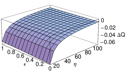
FIG. 3.: Bilepton gauge boson contribution to the anomalous $\Delta Q$ parameter, in units of $a=g^{2}/(96\,\pi^{2})$. $\eta=({M_{Y^{+}}}/m_{W})^{2}$ and $\epsilon=({M^{2}_{Y^{++}}}-{M^{2}_{Y^{+}}})/m_{W}^{2}$.

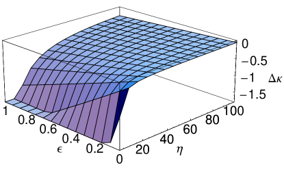
FIG. 4.: Bilepton gauge boson contribution to the anomalous $\Delta\kappa$, in units of $a=g^{2}/(96\,\pi^{2})$. $\eta=({M_{Y^{+}}}/m_{W})^{2}$ and $\epsilon=({M^{2}_{Y^{++}}}-{M^{2}_{Y^{+}}})/m_{W}^{2}$.

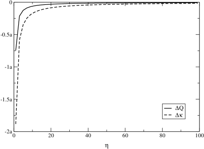
FIG. 5.: Static properties of the $W$ boson, in units of $a=g^{2}/(96\,\pi^{2})$, when the bilepton masses are exactly degenerate, as a function $\eta=(M_{Y}/m_{W})^{2}$.

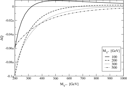
FIG. 6.: Bilepton gauge boson contribution to the anomalous $\Delta Q$ parameter, in units of $a=g^{2}/(96\,\pi^{2})$, as a function of the doubly charged gauge boson mass. We show curves for diverse values of the singly charged gauge boson mass, as indicated in the plot.

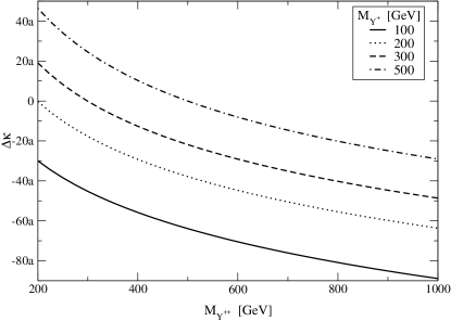
FIG. 7.: Bilepton gauge boson contribution to the anomalous $\Delta\kappa$ parameter, in units of $a=g^{2}/(96\,\pi^{2})$, as a function of the doubly charged gauge boson mass. We show curves for diverse values of the singly charged gauge boson mass, as indicated in the plot.

FIG. 8.: Feynman rules for the trilinear and quartic vertices involving singly and doubly charged gauge bosons. $c_{1}=i\,g/\sqrt{2}$ and the respective expressions for $S$, $T$, $U$ and $V$ are given in Table I.

FIG. 9.: Feynman rules for the trilinear and quartic vertices involving singly and doubly charged pseudo-Goldstone bosons.

FIG. 10.: Feynman rules for the trilinear and quartic vertices involving singly and doubly charged ghost fields.

TABLE I.: Feynman rules for the vertices shown in Fig. 8. $U$ and $U^{\prime}$ stand for the $WWYY$ vertex when $Y=Y^{+}$ and $Y=Y^{++}$, respectively.

	$\mathrm{U_{e}(1)}$-covariant gauge
$S_{\alpha\,\lambda\,\rho}$	$(k_{2}-k_{1})_{\alpha}g_{\lambda\rho}+(k-k_{2})_{\lambda}g_{\alpha\rho}+(k_{1}-k)_{\rho}g_{\alpha\lambda}$
$T_{\alpha\,\lambda\,\rho}$	$(k_{2}-k_{1})_{\alpha}g_{\lambda\rho}+(k-\frac{1}{\xi}\,k_{1}-k_{2})_{\lambda}g_{\alpha\rho}+(k_{1}+\frac{1}{\xi}\,k_{2}-k)_{\rho}g_{\alpha\lambda}$
$U_{\alpha\,\beta\,\lambda\,\rho}$	$g_{\alpha\,\beta}\,g_{\lambda\,\rho}+g_{\alpha\,\rho}\,g_{\beta\,\lambda}-2\,g_{\alpha\,\lambda}\,g_{\beta\,\rho}$
$U^{\prime}_{\alpha\,\beta\,\lambda\,\rho}$	$g_{\alpha\,\beta}\,g_{\lambda\,\rho}-2\,g_{\alpha\,\rho}\,g_{\beta\,\lambda}+g_{\alpha\,\lambda}\,g_{\beta\,\rho}$
$V_{\alpha\,\beta\,\lambda\,\rho}$	$g_{\alpha\,\beta}\,g_{\lambda\,\rho}-\,g_{\alpha\,\rho}\,g_{\beta\,\lambda}$

REFERENCES

- [1] W. A. Bardeen, R. Gastmans, and B. Lautrup, Nucl. Phys. B46, 319 (1972); See also E. N. Argyres, et al., Nucl. Phys. B391, 23 (1993).
- [2] G. Couture and J. N. Ng, Z Phys. C 35, 65 (1987).
- [3] G. Couture, J. N. Ng, J. L. Hewett, and T. G. Rizzo, Phys. Rev. D 36, 859 (1987).
- [4] C. L. Bilachak, R. Gastmans, and A. van Proeyen, Nucl. Phys. B273, 46 (1986); G. Couture, J. N. Ng, J. L. Hewett, and T. G. Rizzo, Phys. Rev. D 38, 860 (1988); A. B. Lahanas and V. C. Spanos, Phys. Lett. B 334, 378 (1994); T. M. Aliyev, Phys. Lett B 155, 364 (1985).
- [5] N. K. Sharma, P. Saxena, Sardar Singh, A. K. Nagawat, and R. S. Sahu, Phys. Rev. D 56, 4152 (1997).
- [6] T. G. Rizzo and M. A. Samuel, Phys. Rev. D 35, 403 (1987); A. J. Davies, G. C. Joshi, and R. R. Volkas, Phys. Rev. D 42, 3226 (1990).
- [7] F. Larios, J. A. Leyva, and R. Martínez, Phys. Rev. D 53, 6686 (1996).
- [8] For a review on the coupling within the effective Lagrangian approach, see J. Ellison and J. Wudka, Annu. Rev. Nucl. Part. Sci. 48, 33 (1998); and references therein.
- [9] F. Pisano and V. Pleitez, Phys. Rev. D 46, 410 (1992); P. H. Frampton, Phys. Rev. Lett. 69, 2889 (1992).
- [10] See for instance G. Tavares-Velasco and J. J. Toscano, Europhys. Lett. 53, 465 (2001).
- [11] T. Appelquist and J. Carazzone, Phys. Rev. D 11, 2856 (1975).
- [12] See for instance J. Collins, F. Wilczek, and A. Zee, Phys. Rev. D 18, 242 (1978); D. Toussaint, Phys. Rev. D 18, 1626 (1978); L. H. Chan, T. Hagiwara, and B. Ovrut, Phys. Rev. D 20, 1982 (1979).
- [13] L. F. Li, Z. Phys. C 58, 519 (1993).
- [14] T. Inami, C. S. Lim, B. Takeuchi, and M. Tanabashi, Phys. Lett. B 381, 458 (1996).
- [15] D. Ng, Phys. Rev. D 49, 4805 (1994).
- [16] G. Passarino and M. Veltman, Nucl. Phys. B160, 151 (1979); see also A. Denner, Fortschr. Phys. 41, 307 (1993).
- [17] R. G. Stuart, Comp. Phys. Commun. 48, 367 (1988); see also G. Devaraj and R.G. Stuart, Nucl. Phys. B519, 483 (2000).
- [18] J. T. Liu and D. Ng, Phys. Rev. D 50, 548 (1994).
- [19] H. N. Long and D. Van Soa, Nucl. Phys. B601, 361 (2001).
- [20] J. T. Liu and D. Ng, Z. Phys. C 62, 693 (1994).
- [21] K. Fujikawa, Phys. Rev. D 7, 393 (1973); M. Baće and N. D. Hari Dass, Ann. Phys. (N. Y.) 94, 349 (1975); M. B. Gavela, G. Girardi, C. Malleville, and P. Sorba, Nucl. Phys. B193, 175 (1981); U. Cotti, J. L. Díaz-Cruz, and J. J. Toscano, Phys. Lett. B 404, 308 (1997); Phys. Rev. D 62, 035009 (1990); J. M. Hernández, M. A. Pérez, G. Tavares-Velasco, and J. J. Toscano, Phys. Rev. D 60, 013004 (1990).
- [22] R. Mertig, M. Böhm and A. Denner, Comp. Phys. Commun. 64, 345 (1991).
- [23] G. t’ Hooft and M. Veltman, Nucl. Phys. B153, 365 (1979).
- [24] G. J. van Oldenborgh, Comput. Phys. Commun. 66 1 (1991); T. Hahn and M. Pérez-Victoria hep-ph/9807565.
- [25] F. Cuypers and S. Davidson, Eur. Phys. J. C 2, 503 (1998); B. Dion, et al., Phys. Rev. D 59, 075006 (1999);
- [26] P. H. Frampton, Int. J. Mod. Phys. A 13, 2345 (1998).
- [27] L. Willmann et al., Phys. Rev. Lett. 82, 49 (1999).
- [28] V. Pleitez, Phys. Rev. D 61 057903 (2000); P. Das and P. Jais, Phys. Rev. D 62, 075001 (2000); P. H. Frampton and A. Rasin, Phys. Lett B. 482, 129 (2000).
- [29] M. B. Tully and G. C. Joshi, Phys. Lett. B 466, 333 (1999).
- [30] E. M. Gregores, A. Gusso, and S. F. Novaes, Phys. Rev. D 64, 015004 (2001).
- [31] M. B. Tully and C. G. Joshi, Int. J. Mod. Phys A 13, 5593 (1998).
- [32] M. Veltman, Nucl. Phys. B123, 89 (1977).
- [33] T. P. Cheng and L. F. Li, Phys. Rev. D 44, 1502 (1991).