Non-Equilibrium Large $N$ Yukawa Dynamics: marching through the Landau pole

Abstract

The non-equilibrium dynamics of a Yukawa theory with N fermions coupled to a scalar field is studied in the large N limit with the goal of comparing the dynamics predicted from the renormalization group improved effective potential to that obtained including the fermionic backreaction. The effective potential is of the Coleman-Weinberg type. Its renormalization group improvement is unbounded from below and features a Landau pole. When viewed self-consistently, the initial time singularity does not arise. The different regimes of the dynamics of the fully renormalized theory are studied both analytically and numerically. Despite the existence of a Landau pole in the model, the dynamics of the mean field is smooth as it passes the location of the pole. This is a consequence of a remarkable cancellation between the effective potential and the dynamical chiral condensate. The asymptotic evolution is effectively described by a quartic upright effective potential. In all regimes, profuse particle production results in the formation of a dense fermionic plasma with occupation numbers nearly saturated up to a scale of the order of the mean field. This can be interpreted as a chemical potential. We discuss the implications of these results for cosmological preheating.

1 Introduction

In the Standard model or its extensions, the Yukawa couplings of Fermions to scalars (Higgs) play a fundamental role. Not only do such couplings determine the masses of the fermionic degrees of freedom, but in turn, it is through these couplings that the fermionic sector influences the dynamics of the scalar fields. If these Yukawa couplings are large enough, they can lead to negative contributions to the beta functions of the running scalar self-couplings and so to destabilizing the vacuum by large negative radiative corrections to the scalar effective potential[1]. This is the Coleman-Weinberg mechanism of symmetry breaking by radiative corrections[2].

While such a scenario has been ruled out within the Standard model due to an unacceptably low value of the Higgs and the top quark masses, large negative radiative corrections to the effective potential from large Yukawa couplings could still be relevant in extensions of the Standard model with more complicated Higgs-Yukawa sectors[3]. Coleman Weinberg phase transitions in extended Higgs models and their potential cosmological implications have been studied by Sher[3] who analyzed the effective potential of this theory. While this study extracted bounds on the parameters of extended Higgs sectors from vacuum stability and thermodynamic considerations, these results are based on an equilibrium description based on the effective potential, a purely static quantity.

Detailed studies reveal that the information extracted from a static effective potential is restricted to situations very close to equilibrium and that a deeper understanding of dynamical processes requires a non-equilibrium treatment. The necessity for a non-equilibrium description of quantum field theory has become clear in cosmology where inflationary phase transitions require a fully dynamical description[4], in heavy-ion collisions where a transient quark-gluon plasma may be formed[5, 6] and domain formation in phase transitions[7, 8] which may have consequences in cosmology as well as in heavy ion collisions.

In each of these fields, non-equilibrium effects can give rise to new phenomena which can differ from equilibrium behavior in dramatic ways that cannot be captured by an effective potential description.

From the point of view of cosmology and inflationary cosmology in particular, non-equilibrium effects associated with particle production via resonances and or instabilities in bosonic field theories have taken center stage. This is evident in the theory of preheating[9] as well as in the classicalization of fluctuations during inflation[10], where spinodally unstable dynamical fluctuations about an homogeneous condensate modify the long wavelength behavior of the theory.

While the non-equilibrium dynamics of fermionic fields has been studied recently by several authors [11, 12, 13, 14] and while there has been some remarkable progress in lattice simulations of fermionic dynamics in low dimensional gauge theories[15], the dynamical behavior of fermions has not received the same level of attention as the bosonic case. This is mostly due to the argument that Fermi-Dirac statistics preclude parametric amplification of occupation numbers with non-perturbative particle production.

In order to have access to non-perturbative dynamics, in this work we consider theories containing $N$ fermions with Yukawa couplings to one scalar field $\Phi$ in leading order in the large $N$ limit. The large $N$ limit leads to a consistent, non-perturbative approximation scheme that can be systematically improved. This approximation has been applied to bosonic theories and has been studied both analytically to leading order[5, 16] and more recently numerically in real time including corrections beyond leading order in the large $N$[17, 18]. These studies reveal a wealth of new phenomena not accessible via perturbative methods.

In the large $N$ limit we study here, the fermions serve to suppress scalar field fluctuations to leading order in $1/N$. We find that even at leading order a new and important aspect of field theory comes into play: the wave function renormalization. It should be noted that this does not occur at the same order in purely scalar theories. Our study reveals that this new ingredient is responsible for dramatic new dynamical phenomena.

We obtain the equations of motion of the mean field, or expectation value of the scalar field, taking into account the non-equilibrium back reaction of the fermionic modes to leading order in $1/N$. This analysis goes beyond the effective potential approximation[2] and affords us a window to understanding the non-perturbative dynamics of this coupled system.

We can summarize our main results as follows:

• The fully renormalized theory displays the Coleman-Weinberg mechanism of dimensional transmutation through radiative corrections. It has an effective potential that is unbounded from below at large values of the mean field with two symmetric global maxima and a local minimum at the origin. It also exhibits a Landau pole at an energy scale $E_{L}$ which is non-perturbative in the Yukawa coupling. The presence of the Landau pole distinguishes two distinct regimes to be studied depending on the relationship between the cutoff $\Lambda$, which is required for the numerical analysis of the theory, and the position $E_{L}$ of the Landau pole.

• Suppose that we take $\Lambda<E_{L}$. Then, if the initial value of the mean field is between the origin and the global maxima, the mean field oscillates about the origin, and the fermionic quantum fluctuations grow as a result of particle production in a preferred band of wave vectors. This is akin to what happens in the bosonic case but here the production must saturate due to Pauli blocking. The width of the band of wave vectors is determined by the initial amplitude of the mean field and the mass of the scalar field. If, however, the initial value of the mean field is larger than the maxima, its amplitude runs away to the cutoff scale at which point the evolution must be stopped since the theory reaches the edge of its domain of validity.

• Our most noteworthy results are those for which $\Lambda>>E_{L}$ and the initial value of the mean field is taken to be larger than the position of the maxima of the effective potential. In this case, an analysis of the dynamics based solely on the static effective potential would lead to the conclusion that the time evolution of the mean field would lead to a divergence or discontinuity in the time derivatives when the amplitude reaches the value of the Landau pole. However a detailed analysis of the full dynamics, including the fermionic fluctuations and their backreaction on to the mean field, reveals that the evolution of the mean field is smooth. When the amplitude of the mean field becomes larger than the Landau pole, the dynamics becomes oscillatory and asymptotically reaches a fixed point described by a simple quartic, upright effective potential with a quartic coupling of order one and with the mean field oscillating with a large amplitude around the origin. This novel dynamical behavior arises from a remarkable cancellation between the fermionic fluctuations and the contribution from the instantaneous effective potential that leads to smooth dynamics through the Landau pole. When the initial value of the mean field is larger than the maxima of the effective potential but much smaller than the Landau pole, the ensuing non-equilibrium evolution leads to fermion production in a band of wave-vectors up to the scale of the Landau pole. These modes become populated with almost Pauli blocking saturation at large times and describe a very dense medium. We study this behavior numerically and confirm that this phenomenon occurs for a wide range of parameters. We are led to conjecture that the theory is, in fact, sensibly behaved beyond the Landau pole when studied both dynamically and non-perturbatively, at least at the mean-field level. While at this point this is merely a conjecture, these phenomena may have some interesting phenomenological consequences.

• A consistent analysis of the renormalization during the dynamical evolution reveals that the wave function renormalization builds up in time over a time scale of ${\cal O}(1/\Lambda)$. The fully renormalized equations of motion display a renormalized coupling at a scale determined by the amplitude of the mean field, and which therefore depends parametrically on time. This is a consequence of the “running” of the coupling constant with scale, which in the dynamical evolution translates to a “running” with time.

The article is organized as follows: in section 2 we obtain the renormalization group improved effective potential, discuss its features including the presence of the Landau pole and the potential singularities that would occur in an analysis based solely on the effective potential. In section 3 we obtain the equations of motion to leading order in the large $N$ limit. In section 4 we address the renormalization of the equations of motion and the energy density. We discuss and resolve the issue of potential initial time singularities; in particular, we highlight the fact that the wave function renormalization builds up on time scales determined by the cutoff. In this section we also establish contact between the non-equilibrium equations of motion and the renormalization group improved effective potential, emphasizing the emergence of smooth dynamics as the mean-field approaches and passes the Landau pole. In section 5 we provide a detailed and comprehensive numerical study of the dynamics in several cases in a wide range of parameters. In section 6 we provide an exact proof of the lack of unstable bands for fermionic mode functions in the background of a scalar field that oscillates, by showing that the Floquet indices are purely real. This is the underlying reason for Pauli blocking at the level of mode functions. We also offer a perturbative analysis of this important phenomenon, which provides the reason for the existence of a preferred band of wave vectors for the produced fermions. We summarize our findings and offer some conjectures for potential implications of our results in cosmology as well as for the phenomenology of theories with extended Higgs-Yukawa sectors containing heavy fermions (and hence large Yukawa couplings) that could feature a Landau pole in an energy range of phenomenological interest.

2 Static aspects: the effective potential and its RG improvement

Before studying the dynamical aspects of the Yukawa theory in the large $N$ limit it is illuminating to understand the static aspects via the effective potential and its renormalization group improvement.

The Yukawa model under consideration is described by the Lagrangian density

$$\mathcal{L} = \frac{1}{2}\left(\partial_{\mu}\Phi_{B}\right)^{2}-\frac{1}{2}m_{B}^{2}\,\Phi_{B}^{2}-\,\frac{\lambda_{B}}{4!\,N}\,\Phi_{B}^{4}$$ (2.1)

$$+\sum_{i=1}^{N}\bar{\psi}_{i}\left[i\gamma^{\mu}\partial_{\mu}-\frac{y_{B}}{\sqrt{N}}\,\Phi_{B}\right]\,\psi_{i},$$

where the subscript $B$ denotes the bare fields, anticipating the need for renormalization. The factors of $N$ in the coupling constants are explicitly displayed so that both the quartic self coupling and the Yukawa coupling are of ${\cal O}(1)$ in the large $N$ limit.

The effective potential is defined as the expectation value of the Hamiltonian in a state that minimizes the energy subject to the constraint that the field has a space-time independent expectation value[19]

$$V_{eff}(\bar{\Phi})=\mbox{min}\frac{\langle\bar{\Phi}|H|\bar{\Phi}\rangle}{\Omega}$$ (2.2)

with $\Omega$ the spatial volume and $|\bar{\Phi}\rangle$ a (coherent) state for which

$$\langle\bar{\Phi}|\Phi|\bar{\Phi}\rangle=\bar{\Phi}.$$ (2.3)

To leading order in the large $N$ the effective potential is obtained by replacing $\Phi(\vec{x})\rightarrow\bar{\Phi}$ in the Hamiltonian and neglecting the scalar field fluctuations, since the energy will be dominated by the $N$ fermion fields. This is the mean field approximation, which becomes exact in the large $N$ limit.

Hence

$$H[\bar{\Phi}]=\Omega\left(\frac{1}{2}m_{B}^{2}\,{\bar{\Phi}}^{2}+\,\frac{\lambda_{B}}{4!\,N}\,{\bar{\Phi}}^{4}\right)+\sum_{i=1}^{N}\bar{\psi}_{i}\left[-i\vec{\alpha}\cdot\vec{\triangledown}+M\right]\,\psi_{i},$$ (2.4)

$$M=\frac{y_{B}}{\sqrt{N}}\bar{\Phi}.$$ (2.5)

The fermionic contribution to the Hamiltonian is simply that of $N$ Dirac fermions of mass $M$, and can be diagonalized in terms of creation and annihilation operators for particles and antiparticles with dispersion relation $\omega_{k}=\sqrt{k^{2}+M^{2}}$. The state that minimizes the expectation value of the normal ordered Hamiltonian is the vacuum state for particles and antiparticles and corresponds to the Dirac sea completely filled (with two spin states per wave vector). It is convenient to rescale the expectation value of the scalar field to exhibit the large $N$ limit more clearly:

$$\bar{\Phi}=\sqrt{N}~{}\delta_{B}$$ (2.6)

in terms of which

$$V_{eff}(\delta)=N\left\{\frac{m_{B}^{2}}{2}\delta^{2}_{B}+\frac{\lambda_{B}}{4!}\delta^{4}_{B}-2\int\frac{d^{3}k}{(2\pi)^{3}}\sqrt{k^{2}+M^{2}}\right\}.$$ (2.7)

The integral in (2.7) is the (negative) contribution from the Dirac sea, and is calculated with an ultraviolet cutoff $\Lambda$. A straightforward calculation, subtracting the “zero point energy” $\propto\Lambda^{4}$ and neglecting terms that vanish in the limit $\Lambda\rightarrow\infty$, leads to

$$\frac{V_{eff}(\delta)}{N}= \frac{\delta^{2}_{B}}{2}\left(m^{2}_{B}-\frac{y^{2}_{B}\Lambda^{2}}{4\pi^{2}}\right)+\frac{\delta^{4}_{B}}{4}\left(\frac{\lambda_{B}}{3!}+\frac{y^{4}_{B}}{2\pi^{2}}\ln\left[\frac{2\Lambda}{\mu}\right]\right)$$ (2.8)

$$-\frac{y^{4}_{B}~{}\delta^{4}_{B}}{8\pi^{2}}\ln\left[\left|\frac{y_{B}~{}\delta_{B}}{\mu}\right|\right]-\frac{y^{4}_{B}\delta^{4}_{B}}{32\pi^{2}},$$

where $\mu$ is an arbitrary renormalization scale. The renormalization of the mass and quartic scalar coupling $\lambda$ can be gleaned directly from the form of the effective potential above. However, to make contact with the dynamics in which the equations of motion are obtained from the non-equilibrium effective action, we also need the field or wave function renormalization. The wave function renormalization cannot be extracted from the effective potential since it is associated with gradient terms in the effective action. To leading order in $1/N$ it can be obtained from the one-fermion loop self energy shown in figure (1) below, where the scalar field lines have non-vanishing external momentum.

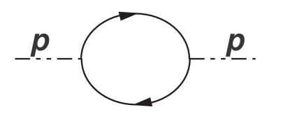
Figure 1: Scalar self energy in leading order in large $N$. External dashed lines correspond to the scalar field, internal solid lines are fermions.

This calculation leads to

$$Z[\mu]=\left(1+\frac{y^{2}_{B}}{4\pi^{2}}\ln\left[\frac{2\Lambda}{\mu}\right]\right)^{-1}.$$ (2.9)

The renormalization of field, mass and couplings is now achieved by introducing

$$\delta_{R} = \frac{\delta_{B}}{\sqrt{Z}},$$ (2.10)

$$m^{2}_{R} = Z\left(m^{2}_{B}-\frac{y^{2}_{B}\Lambda^{2}}{2\pi^{2}}\right),$$ (2.11)

$$\frac{\lambda_{R}}{3!} = Z^{2}\left(\frac{\lambda_{B}}{3!}+\frac{y^{4}_{B}}{2\pi^{2}}\ln\left[\frac{2\Lambda}{\mu}\right]\right),$$ (2.12)

$$y_{R} = y_{B}\sqrt{Z},$$ (2.13)

in terms of which the renormalized effective potential is given by

$$V_{eff}(\delta_{R})=\frac{1}{2}m^{2}_{R}~{}\delta^{2}_{R}+\frac{\delta^{4}_{R}}{4}\left(\frac{\lambda_{R}}{3!}-\frac{y^{4}_{R}}{2\pi^{2}}\ln\left|\frac{y_{R}~{}\delta_{R}e^{\frac{1}{4}}}{\mu}\right|\right).$$ (2.14)

We will consider the case in which the renormalized mass of the scalar field vanishes, since this case will highlight the important feature of dimensional transmutation both at the level of the static effective potential as well as the dynamics. Therefore in what follows we set $m_{R}=0$.

The equation of motion, which will be the focus of next section, requires $V^{\prime}(\delta_{R})=\partial V(\delta_{R})/\partial\delta_{R}$. This is given by

$$V^{\prime}(\delta_{R})=\frac{y^{4}_{R}}{2\pi^{2}}\delta^{3}_{R}\left[\frac{2\pi^{2}\lambda_{R}}{3!y^{4}_{R}}-\ln\left[\frac{|M_{R}|}{\mu}\right]-\frac{1}{2}\right],$$ (2.15)

where we introduced the renormalized effective fermion mass

$$M_{R}=y_{R}\delta_{R}.$$ (2.16)

We see that the effective potential features an extremum at $M_{R}={\bar{M}}$ with ${\bar{M}}$ determined by

$$\left[\frac{2\pi^{2}\lambda_{R}}{3!y^{4}_{R}}-\ln\left[\frac{|{\bar{M}}|}{\mu}\right]-\frac{1}{2}\right]=0.$$ (2.17)

In terms of the scale ${\bar{M}}$ we find

$$V^{\prime}_{eff}(\delta_{R}) = -\frac{y^{4}_{R}\delta^{3}_{R}}{2\pi^{2}}\ln\left[\frac{|M_{R}|}{{\bar{M}}}\right],$$ (2.18)

$$V_{eff}(\delta_{R}) = -\frac{y^{4}_{R}\delta^{4}_{R}}{8\pi^{2}}\ln\left[\frac{|M_{R}|e^{-\frac{1}{4}}}{{\bar{M}}}\right].$$ (2.19)

Thus we see that the term $\lambda_{R}/3!$ inside the parenthesis in (2.14) above has been traded for a new scale ${\bar{M}}$ at which the effective potential features a maximum. This is the manifestation of dimensional transmutation[2].

Figure (2) below displays $V_{eff}/{\bar{M}}^{4}$ vs. $\chi=\frac{M_{R}}{{\bar{M}}}$. The $V_{eff}$ is given by (2.19).

Figure 2: $F(\chi)=-\chi^{4}\ln(|\chi|e^{-\frac{1}{4}})$ vs. $\chi=\frac{M_{R}}{\bar{M}}$

While there are alternative calculations of the effective potential, the Hamiltonian formulation highlights many important aspects that will be relevant to the discussion in the next sections. In particular, it makes clear that the effective potential is the expectation value of the Hamiltonian in a “vacuum” state in which the scalar field attains an expectation value. Furthermore, this Hamiltonian interpretation immediately provides the physical reason for the effective potential being unbounded below in this approximation: it is completely determined by the negative energy Dirac sea. For larger amplitudes of the expectation value, the effective fermionic mass $M_{R}$ is larger, thus the negative energy of a free fermion mode of momentum $k$ in the Dirac sea decreases further. Thus for larger amplitudes of the expectation value, the energy stored in the Dirac sea becomes more negative. This particular point should be borne in mind when we study the dynamics of the mean field below, since we will find that the evolution of the scalar field “feeds off” the negative energy Dirac sea.

2.1 RG improvement:

The emergence of the scale ${\bar{M}}$ is a consequence of the renormalization scale $\mu$ introduced above. A change in this scale is compensated for by a change in the couplings. The effective action

$$\Gamma[\delta_{R}]=\int d^{4}x\left[-V_{eff}[\delta_{R}]+{\cal Z}[\delta_{R}]\frac{1}{2}(\partial_{\mu}\delta_{R})^{2}+\cdots\right]$$ (2.20)

is invariant under a change of the renormalization scale, and consequently under a change in the scale ${\bar{M}}$. This invariance leads to a renormalization group equation for the effective action[2].

Since our main focus is to study dynamical behavior, which involves $V^{\prime}_{eff}$, we now use the renormalization group to improve the derivative of the effective potential.

While in principle we can study the full solution of the renormalization group equation as in[2], the large $N$ approximation simplifies the task. In this limit we need only keep the one loop fermion contribution to renormalization. Therefore, after trading the quartic self-coupling for the scale ${\bar{M}}$ via dimensional transmutation, the effective potential (and its derivatives) are only functions of the Yukawa coupling. Furthermore, from the renormalization conditions (2.10,2.13) the product $y_{R}\delta_{R}$ is a renormalization group invariant, i.e, is constant under a change of scales. With the purpose of comparing with the dynamics to be studied in the next section, it is convenient to introduce the coupling

$$g_{R}(\mu)=\frac{y^{2}_{R}(\mu)}{2\pi^{2}},$$ (2.21)

and to RG improve the product

$$y_{R}(\mu)V^{\prime}_{eff}(\delta_{R}(\mu))=-g_{R}(\mu)M^{3}_{R}\ln|\frac{M_{R}}{\bar{M}}|.$$ (2.22)

The reason for studying this product is based on the idea that the effective equation of motion of the scalar field is loosely of the form

$$\ddot{\delta}_{R}(t)+V^{\prime}_{eff}(\delta_{R}(t))=0.$$ (2.23)

While $\delta$ is not invariant under a change of scale (i.e, under a renormalization group transformation) in the large $N$ limit the product $M_{R}=y_{R}\delta_{R}$ is a renormalization group invariant. Thus one is led to consider the product $y_{R}V^{\prime}_{eff}$.

However, from the renormalization condition (2.13) of the Yukawa coupling and the wave-function renormalization constant in the large $N$ limit given by (2.9) we find

$$\frac{2}{g_{R}(\mu)}=\frac{2}{g_{B}}+\ln\left[\frac{2\Lambda}{\mu}\right],$$ (2.24)

which leads to the renormalization group running of this coupling

$$\frac{2}{g_{R}(\mu^{\prime})}=\frac{2}{g_{R}(\mu)}+\ln\left[\frac{\mu}{\mu^{\prime}}\right].$$ (2.25)

Therefore choosing the new scale $\mu^{\prime}\equiv M_{R}$ with the scale of dimensional transmutation ${\bar{M}}$ fixed, the renormalization group improvement of the product (2.22) leads to

$$y_{R}(|M_{R}|)V^{\prime}_{eff}(M_{R})=-g_{R}(|M_{R}|)M^{3}_{R}\ln\left|\frac{M_{R}}{\bar{M}}\right|=-\frac{g~{}{\bar{M}}^{3}\chi^{3}~{}\ln|\chi|}{(1-\frac{g}{2}\ln|\chi|)},$$ (2.26)

with $g=g_{R}({\bar{M}})~{},~{}\chi=M_{R}/{\bar{M}}$.

The expression (2.26) features a Landau pole at

$$M_{R}\sim{\bar{M}}e^{\frac{2}{g}}$$ (2.27)

which, if interpreted in terms of the equation of motion of the scalar field via the effective action (2.20) would signal infinite time derivatives when the value of the scalar field reaches the putative Landau pole. Since the large $N$ limit does not restrict the coupling to be weak, the value of $g$ can be ${\cal O}(1)$. Therefore if the dynamical evolution of the expectation value of the scalar field is solely determined by $V^{\prime}_{eff}$ we would expect large derivatives and non-analytic behavior of the dynamics as the scalar field approaches the position of the Landau pole.

An important result of this work is that the Landau pole is not relevant for the dynamical evolution of the scalar field and contributions from particle production that cannot be captured by the effective potential become very important. These non-equilibrium contributions lead to smooth dynamics as the expectation value of the scalar field nears the Landau pole.

3 Large N Yukawa Dynamics

Having studied the static aspects of the Yukawa theory in the large $N$ limit via the effective potential and its renormalization group improvement, we now focus our attention on the dynamical aspects of this model.

As discussed in the introduction, we consider a system of $N$ fermions $\left\{\psi_{i}\right\}_{i=1}^{N}$ coupled to a scalar field $\Phi$. The Lagrangian density in terms of bare fields, mass and couplings is given by equation (2.1) above. In order to study the dynamics as an initial value problem we introduce an external “magnetic field” coupled to the scalar field so that ${\cal L}\rightarrow{\cal L}+h(t)\Phi_{B}$ with ${\cal L}$ the Lagrangian density in (2.1). The external source $h(t)$ serves to generate a spatially homogeneous expectation value for the scalar field

We will assume that the source was switched on adiabatically in the infinite past and then slowly switched off at $t=0$. This means that the scalar field evolves in the absence of this external source for $t\geq 0$. This adiabatic switching on procedure allows us to establish a connection with the effective potential formalism of the previous section. If the initial state as $t\rightarrow-\infty$ is the vacuum, an adiabatically switched on source ensures that the state is the adiabatic vacuum; recall that the (zero temperature) effective potential is referred to the expectation value of the field in the vacuum state. We will discuss this issue in greater detail below when we address the renormalization aspects.

In order to extract the dynamics of the mean field, we expand the scalar field as $\Phi_{B}\left(\vec{x},t\right)=\sqrt{N}\,\delta_{B}\left(t\right)+\chi\left(\vec{x},t\right)$ with $\left\langle\chi\left(\vec{x},t\right)\right\rangle=0$. Implementing this last equation within the path integral via the tadpole method[12], we find that to leading order in $1/N$, we arrive at the following equation of motion for the mean field $\delta_{B}\left(t\right)$:

$$\ddot{\delta}_{B}\left(t\right)+m_{B}^{2}\,\delta_{B}\left(t\right)+\frac{\lambda_{B}}{3!}\delta_{B}^{3}\left(t\right)+\frac{y_{B}}{N}\sum_{i=1}^{N}\left\langle\bar{\psi}_{i}\,\psi_{i}\right\rangle=h(t).$$ (3.1)

Note that this equation is non-perturbatively exact in the $N\rightarrow\infty$ limit. The Dirac equations for the $N$ species of fermions $\psi_{i}$ are :

$$\left(i\,\gamma^{\mu}\partial_{\mu}-M_{B}\left(t\right)\right)\psi_{i}=0\text{, where }M_{B}\left(t\right)=y_{B}\,\delta_{B}\left(t\right)\text{.}$$ (3.2)

The above equations are invariant under a permutation of the fermion fields so that we need only deal with one of them, denoted generically as $\psi$; therefore we make the replacement

$$\frac{y_{B}}{N}\sum_{i=1}^{N}\left\langle\bar{\psi}_{i}\,\psi_{i}\right\rangle\rightarrow y_{B}\left\langle\bar{\psi}\psi\right\rangle$$ (3.3)

in eq.(3.1).

In order to proceed, we expand the spinor field operators in terms of a complete set of mode functions solutions of the time dependent Dirac equation into eq.(3.2):

$$\psi\left(\vec{x},t\right)=\sum_{\alpha=1}^{2}\int\frac{d^{3}p}{\left(2\pi\right)^{3}}\left[b_{\vec{p},\alpha}\,U_{\vec{p}}^{\left(\alpha\right)}\left(t\right)\,e^{i\,\vec{p}\cdot\vec{x}}+d_{\vec{p},\alpha}^{\dagger}\,V_{\vec{p}}^{\left(\alpha\right)}\left(t\right)\,e^{-i\,\vec{p}\cdot\vec{x}}\right],$$ (3.4)

where the creation/annihilation operators obey the usual anticommutation relations

$$\left\{b_{\vec{p},\alpha},b_{\vec{q},\beta}^{\dagger}\right\}=\left\{d_{\vec{p},\alpha},d_{\vec{q},\beta}^{\dagger}\right\}=\left(2\pi\right)^{3}\,\delta_{\alpha\beta}\,\delta^{\left(3\right)}\left(\vec{p}-\vec{q}\right),$$ (3.5)

and the Dirac spinors satisfy the completeness relation

$$\sum_{\alpha=1}^{2}\left[U_{\vec{p}}^{\left(\alpha\right)}\left(t\right)_{a}\,U_{\vec{p}}^{\left(\alpha\right)\dagger}\left(t\right)_{b}+V_{-\vec{p}}^{\left(\alpha\right)}\left(t\right)_{a}\,V_{-\vec{p}}^{\left(\alpha\right)\dagger}\left(t\right)_{b}\right]=\delta_{ab},$$ (3.6)

with $a,b$ being Dirac space indices. Furthermore, eq.(3.2) implies:

$$\left(i\,\gamma^{0}\partial_{0}-\vec{\gamma}\cdot\vec{p}-M_{B}\left(t\right)\right)U_{\vec{p}}^{\left(\alpha\right)}\left(t\right)=0,\text{ }\left(i\,\gamma^{0}\partial_{0}+\vec{\gamma}\cdot\vec{p}-M_{B}\left(t\right)\right)V_{\vec{p}}^{\left(\alpha\right)}\left(t\right)=0.$$ (3.7)

Since the time derivative operator $\partial_{0}$ is singled out by our need to consider the time evolution of the system, it is best to work in the basis in which $\gamma^{0}$ is diagonal. Writing the four-component spinors $U_{\vec{p}}^{\left(\alpha\right)}\left(t\right)$, $V_{\vec{p}}^{\left(\alpha\right)}\left(t\right)$ in terms of two-component spinors $\chi_{i\vec{p}}^{\left(\alpha\right)},\xi_{i\vec{p}}^{\left(\alpha\right)}$ , $i=1,2$:

$$U_{\vec{p}}^{\left(\alpha\right)}\left(t\right)=\left(\begin{array}[c]{c}f_{1\,\vec{p}}\left(t\right)\,\chi_{1\vec{p}}^{\left(\alpha\right)}\\ f_{2\,\vec{p}}\left(t\right)\,\chi_{2\vec{p}}^{\left(\alpha\right)}\end{array}\right),\,V_{\vec{p}}^{\left(\alpha\right)}\left(t\right)=\left(\begin{array}[c]{c}g_{1\,\vec{p}}\left(t\right)\,\xi_{1\vec{p}}^{\left(\alpha\right)}\\ g_{2\,\vec{p}}\left(t\right)\,\xi_{2\vec{p}}^{\left(\alpha\right)}\end{array}\right),$$ (3.8)

we can use eq.(3.7) to find:

$$\left(i\,\partial_{0}-M_{B}\left(t\right)\right)f_{1\,\vec{p}}\left(t\right)\,\chi_{1\vec{p}}^{\left(\alpha\right)} =\left(\vec{\sigma}\cdot\vec{p}\right)f_{2\,\vec{p}}\left(t\right)\,\chi_{2\vec{p}}^{\left(\alpha\right)}$$ (3.9)

$$\left(i\,\partial_{0}+M_{B}\left(t\right)\right)f_{2\,\vec{p}}\left(t\right)\,\chi_{2\vec{p}}^{\left(\alpha\right)} =\left(\vec{\sigma}\cdot\vec{p}\right)f_{1\,\vec{p}}\left(t\right)\,\chi_{1\vec{p}}^{\left(\alpha\right)},$$

$$\left(i\,\partial_{0}-M_{B}\left(t\right)\right)g_{1\,\vec{p}}\left(t\right)\,\xi_{1\vec{p}}^{\left(\alpha\right)} =-\left(\vec{\sigma}\cdot\vec{p}\right)g_{2\,\vec{p}}\left(t\right)\,\,\xi_{2\vec{p}}^{\left(\alpha\right)}$$ (3.10)

$$\left(i\,\partial_{0}+M_{B}\left(t\right)\right)g_{2\,\vec{p}}\left(t\right)\,\,\xi_{2\vec{p}}^{\left(\alpha\right)} =-\left(\vec{\sigma}\cdot\vec{p}\right)g_{1\,\vec{p}}\left(t\right)\xi_{1\vec{p}}^{\left(\alpha\right)}.$$

We also impose the normalization conditions

$$U_{\vec{p}}^{\left(\alpha\right)\dagger}\left(t\right)U_{\vec{p}}^{\left(\beta\right)}\left(t\right)=\delta^{\alpha\beta}=V_{\vec{p}}^{\left(\alpha\right)\dagger}\left(t\right)V_{\vec{p}}^{\left(\beta\right)}\left(t\right),$$ (3.11)

which together with $\chi_{i\vec{p}}^{\left(\alpha\right)\dagger}\,\chi_{i\vec{p}}^{\left(\alpha\right)}=\delta^{\alpha\beta}$, $i=1,2,$ imply that

$$\left|f_{1\,\vec{p}}\left(t\right)\right|^{2}+\left|f_{2\,\vec{p}}\left(t\right)\right|^{2}=1$$ (3.12)

which is a consequence of the conservation of probability in the Dirac theory, which in turn is a consequence of the fact that the Dirac equation is first order in time. This constraint on the mode functions will have important consequences in the dynamics and underlies the mechanism of Pauli blocking, as will be analyzed in detail below.

We determine the initial state by demanding that $U_{\vec{p}}^{\left(\alpha\right)}\left(t=0\right)$ represent positive energy states while $V_{\vec{p}}^{\left(\alpha\right)}\left(t=0\right)$ represent negative energy ones:

$$i\,\partial_{0}U_{\vec{p}}^{\left(\alpha\right)}\left(t=0\right)=\omega_{p}\left(t=0\right)U_{\vec{p}}^{\left(\alpha\right)}\left(t<0\right),\,$$ (3.13a)

$$i\,\partial_{0}V_{\vec{p}}^{\left(\alpha\right)}\left(t=0\right)=-\omega_{p}\left(t=0\right)V_{\vec{p}}^{\left(\alpha\right)}\left(t=0\right)\,,$$ (3.13b)

where $$\omega_{p}\left(t\right)=\sqrt{p^{2}+M_{B}\left(t\right)^{2}} t=0 t=0$$ are the mode frequencies. Considering an initial state for which the time derivative of the scalar field vanishes at (which can always be achieved by a shift in the time variable) and then evaluating eqs.(3.9,3.10) at and using eqs.(3.13), we find:

$$\left(\omega_{0}-M_{0}\right)\,f_{1\,\vec{p}}\left(0\right)\,\chi_{1\vec{p}}^{\left(\alpha\right)} =\left(\vec{\sigma}\cdot\vec{p}\right)\,f_{2\,\vec{p}}\left(0\right)\,\chi_{2\vec{p}}^{\left(\alpha\right)}$$ (3.14)

$$\left(\omega_{0}+M_{0}\right)\,f_{2\,\vec{p}}\left(0\right)\,\chi_{2\vec{p}}^{\left(\alpha\right)} =\left(\vec{\sigma}\cdot\vec{p}\right)\,f_{1\,\vec{p}}\left(0\right)\,\chi_{1\vec{p}}^{\left(\alpha\right)},$$ (3.15)

where $\omega_{0}=\omega_{p}\left(0\right)$, $M_{0}=M_{B}\left(0\right)$. This leads to the relations:

$$f_{1\,\vec{p}}\left(0\right)=\sqrt{\frac{\omega_{0}+M_{0}}{2\,\omega_{0}}},\,f_{2\,\vec{p}}\left(0\right)=\sqrt{\frac{\omega_{0}-M_{0}}{2\,\omega_{0}}},\,\chi_{2\vec{p}}^{\left(\alpha\right)}=\left(\vec{\sigma}\cdot\hat{p}\right)\chi_{1\vec{p}}^{\left(\alpha\right)}.$$ (3.16)

A similar analysis for the negative energy modes shows that in fact $g_{1\,\vec{p}}\left(t\right)=f_{2\,\vec{p}}^{\ast}\left(t\right),$ $g_{2\,\vec{p}}\left(t\right)=f_{1\,\vec{p}}^{\ast}\left(t\right),\,\xi_{2\vec{p}}^{\left(\alpha\right)}=\left(\vec{\sigma}\cdot\hat{p}\right)\,\xi_{1\vec{p}}^{\left(\alpha\right)}$ so that we only need to solve for the positive energy modes. Using the relation between the spinors in (3.16), equations (3.9) reduce to:

$$\left(i\,\partial_{0}-M_{B}\left(t\right)\right)f_{1\,\vec{p}}\left(t\right) =pf_{2\,\vec{p}}$$ (3.17)

$$\left(i\,\partial_{0}+M_{B}\left(t\right)\right)f_{2\,\vec{p}}\left(t\right) =pf_{1\,\vec{p}}\;.$$

These can be seperated into two second order equations:

$$\left(\partial_{0}^{2}+p^{2}+M^{2}_{B}(t)\pm i\,\dot{M}_{B}\left(t\right)\right)\,f_{1,2\ \vec{p}}\left(t\right)=0.$$ (3.18)

The second order equations have twice as many solutions as the first order equations, but since the initial conditions for these equations are determined from the first order equations, the correct, physical, pair of solutions will be found. The second order equations are of interest because they are more amenable to the WKB expansion in the next section.

The quantity $\left\langle\bar{\psi}\psi\right\rangle$ appears in the mean field equation eq.(3.1); we need to calculate it in terms of the mode functions $\left\{f_{1\,\vec{p}}\left(t\right),\,f_{2\,\vec{p}}\left(t\right)\right\}$. This is easily done for our state when we note that $\left\langle b_{\vec{q},\alpha}^{\dagger}\,b_{\vec{p},\beta}\right\rangle=0$  while $\left\langle d_{\vec{p},\alpha}\,d_{\vec{q},\alpha}^{\dagger}\,\right\rangle=\left\langle\left\{d_{\vec{p},\alpha},\,d_{\vec{q},\beta}^{\dagger}\right\}\,\right\rangle=\left(2\pi\right)^{3}\,\delta_{\alpha\beta}\,\delta^{\left(3\right)}\left(\vec{p}-\vec{q}\right)$ and use $g_{1\,\vec{p}}\left(t\right)=f_{2\,\vec{p}}^{\ast}\left(t\right),$ $g_{2\,\vec{p}}\left(t\right)=f_{1\,\vec{p}}^{\ast}\left(t\right)$:

$$\left\langle\bar{\psi}\psi\right\rangle=2\,\int\frac{d^{3}p}{\left(2\pi\right)^{3}}\left(\left|\,f_{2\,\vec{p}}\left(t\right)\right|^{2}-\left|\,f_{1\,\vec{p}}\left(t\right)\right|^{2}\right).$$ (3.19)

Another important quantity for us is the energy density $\rho_{\text{f}}$ in the fermionic fluctuations:

$$\rho_{\text{f}}\equiv\left\langle T_{0}^{0}\right\rangle=\frac{i}{2}\left\langle\psi^{\dagger}\,\dot{\psi}-\dot{\psi}^{\dagger}\,\psi\,\right\rangle=2\,\int\frac{d^{3}p}{\left(2\pi\right)^{3}}\Im m\left(f_{1\,\vec{p}}^{\ast}\left(t\right)\,\dot{f}_{1\,\vec{p}}\left(t\right)+f_{2\,\vec{p}}^{\ast}\left(t\right)\,\dot{f}_{2\,\vec{p}}\left(t\right)\right),$$ (3.20)

where $T_{0}^{0}$ is the indicated component of the fermionic stress energy tensor operator.

At this point it is important to highlight the connection with the static effective potential studied in section 2 above.

The equation of motion for the mean field eqn. (3.1) suggests the identification of the fermionic contribution, the last term of (3.1), with the derivative of the fermionic contribution to the effective potential (divided by $N$) given by eqn. (2.7). Such an identification, however, could only hold for a time independent mean field. Indeed in this case, when the scalar field is independent of time, the solutions of the mode equations with the initial conditions given in eqn. (3.16) are given by $f_{1,{\vec{p}}}(t)=f_{1,{\vec{p}}}(0);f_{2,{\vec{p}}}(t)=f_{2,{\vec{p}}}(0)$ leading to

$$\langle{\bar{\psi}}\psi\rangle|_{\text{static}}=-2\int\frac{d^{3}k}{(2\pi)^{3}}\frac{M_{B}}{\sqrt{k^{2}+M^{2}_{B}}},$$ (3.21)

which is the derivative of the fermionic contribution to the effective potential with respect to the effective mass $M_{B}$. Thus the connection with the effective potential for a static mean field is manifest. As it will be explained in detail below, for a dynamically evolving mean field there are non-equilibrium contributions that cannot be captured by the static effective potential and that are responsible for a wealth of new phenomena associated with the non-equilibrium dynamics.

4 WKB Expansion and Renormalization

While the renormalization aspects of the Yukawa theory to leading order in the large $N$ approximation have been studied previously [11, 12], here we provide an alternative method, based on the WKB expansion, that makes contact with the effective potential formalism studied in section (2) above.

4.1 WKB Solution of the Mode Equations

Both the chiral condensate $\left\langle\bar{\psi}\psi\right\rangle$ and the energy density $\rho_{\text{f}}$ are divergent. In order to construct the renormalized equations of motion, we need to extract their divergent parts so that they can be absorbed by appropriate counterterms. This can be done by finding solutions to eq.(3.18) that allow for a large momentum expansion, i.e. a WKB expansion. We will concentrate on $f_{2\,\vec{p}}\left(t\right)$ since the results for $f_{1\,\vec{p}}\left(t\right)$ can be then be obtained via the replacement $M_{B}\left(t\right)\leftrightarrow-M_{B}\left(t\right)$ throughout, including in the initial conditions.

The WKB ansatz for $f_{2\,\vec{p}}\left(t\right)$ is:

$$f_{2}^{\left(I\right)}\left(t\right)=A\left(t\right)\,\exp\,i\,\int_{0}^{t}du\,\Omega\left(u\right)\,,$$ (4.1)

where from now on we omit the $\vec{p}$ index on the mode functions. Insert this into eq.(3.18) and take the real and imaginary parts to find:

$$\frac{\ddot{A}\left(t\right)}{A\left(t\right)}+\omega_{\vec{p}}^{2}\left(t\right)=\Omega^{2}\left(t\right);\,\,2\frac{\dot{A}\left(t\right)}{A\left(t\right)}+\frac{\dot{\Omega}\left(t\right)}{\Omega\left(t\right)}=\frac{\dot{M}_{B}\left(t\right)}{\Omega\left(t\right)}.$$ (4.2)

We can solve these equations:

$$f_{2}^{\left(I\right)}\left(t\right)=\frac{1}{\sqrt{2\,\Omega\left(t\right)}}\,\exp\,\int_{0}^{t}du\,\left(i\Omega\left(u\right)+\frac{\dot{M}_{B}\left(u\right)}{2\,\Omega\left(u\right)}\right),\text{ where }$$ (4.3)

$$\Omega^{2}\left(t\right)=\omega_{\vec{p}}^{2}\left(t\right)+\left(\frac{3}{4}\left(\frac{\dot{\Omega}\left(t\right)}{\Omega\left(t\right)}\right)^{2}-\frac{1}{2}\left(\frac{\ddot{\Omega}\left(t\right)}{\Omega\left(t\right)}\right)\right)+$$ (4.4)

$$\left(\frac{1}{2}\left(\frac{\ddot{M}_{B}\left(t\right)}{\Omega\left(t\right)}\right)+\frac{1}{4}\left(\frac{\dot{M}_{B}\left(t\right)}{\Omega\left(t\right)}\right)^{2}-\frac{\dot{M}_{B}\left(t\right)\,\dot{\Omega}\left(t\right)}{\Omega\left(t\right)^{2}}\right).$$

Given $f_{2}^{\left(I\right)}\left(t\right)$, the second,linearly independent, solution $f_{2}^{\left(II\right)}\left(t\right)$ is:

$$f_{2}^{\left(II\right)}\left(t\right) =\,f_{2}^{\left(I\right)}\left(t\right)\,F\left(t\right),$$ (4.5)

$$F\left(t\right) =-i\int_{0}^{t}\frac{du\,}{f_{2}^{\left(I\right)}\left(u\right)^{2}}.$$

Without loss of generality we can take the lower limit of integration in $F\left(t\right)$ to be $t=0$, since including an arbitrary constant in $F\left(t\right)$ will only give rise to a part proportional to $f_{2}^{\left(I\right)}\left(t\right)$ in $f_{2}^{\left(II\right)}\left(t\right)$. This in turn can be absorbed when constructing the appropriate linear combination to satisfy the initial conditions. The overall factor of $-i$ was chosen so that the Wronskian of $f_{2}^{\left(I\right)}\left(t\right)$, $f_{2}^{\left(II\right)}\left(t\right)$ would coincide with its value in the equilibrium case.

Write $f_{2}\left(t\right)=A_{I}\,f_{2}^{\left(I\right)}\left(t\right)+A_{II}\,f_{2}^{\left(II\right)}\left(t\right)$, and impose the conditions

$$f_{2}\left(0\right)=\sqrt{\frac{\omega_{0}-M_{0}}{2\,\omega_{0}}}\quad\quad,\quad\quad i\,\dot{f}_{2}\left(0\right)=\omega_{0}f_{2}\left(0\right)$$ (4.6)

to find:

$$f_{2}\left(t\right)=f_{2}\left(0\right)\left\{\frac{f_{2}^{\left(I\right)}\left(t\right)}{f_{2}^{\left(I\right)}\left(0\right)}\left[1+\left(\omega_{0}+\Omega\left(0\right)-i\frac{\dot{M}\left(0\right)-\dot{\Omega}\left(0\right)}{2\Omega\left(0\right)}\right)f_{2}^{\left(I\right)}\left(0\right)^{2}F\left(t\right)\right]\right\}.$$ (4.7)

4.2 Renormalizing $\left\langle\bar{\psi}\psi\right\rangle$

We begin the renormalization program by first studying the divergences in the fermion (chiral) condensate $\left\langle\bar{\psi}\psi\right\rangle$. The ultraviolet divergences of this expectation value can be extracted by performing a high momentum expansion of $\left|f_{2}\left(t\right)\right|^{2}-$ $\left|f_{1}\left(t\right)\right|^{2}$; the only terms that will be relevant are those proportional to $1/k^{p}$, $0\leq p\leq 3$ for large $k$. An alternative formulation can be found in references[20, 11]. Furthermore, since we can obtain $f_{1}\left(t\right)$ from $f_{2}\left(t\right)$ by making the replacement $M_{B}\left(t\right)\leftrightarrow-M_{B}\left(t\right)$, $\left|f_{2}\left(t\right)\right|^{2}-$ $\left|f_{1}\left(t\right)\right|^{2}$ is odd in $M_{B}\left(t\right)$.

We first solve for the WKB frequencies by iterating eq.(4.4) once and keeping the appropriate power of the momentum in the large momentum limit:

$$\Omega^{\left(0\right)}\left(t\right) =\omega\left(t\right)$$ (4.8)

$$\Omega^{\left(2\right)}\left(t\right) =\omega\left(t\right)\left(1+\frac{\ddot{M}_{B}\left(t\right)}{4\omega\left(t\right)^{3}}\right).$$ (4.9)

We will also need the high momentum behavior of $F\left(t\right)$ as defined in eq.(4.5). This is most easily obtained by integrating by parts a sufficient number of times to extract the relevant part. Doing this for $\left\langle\bar{\psi}\psi\right\rangle$, we find

$$F\left(t\right)=-1-i\frac{\dot{M}_{B}\left(0\right)}{2\Omega\left(0\right)^{2}}-\frac{\ddot{M}_{B}\left(0\right)}{4\Omega\left(0\right)^{3}}+$$ (4.10)

$$\left(1+i\frac{\dot{M}_{B}\left(t\right)}{2\Omega\left(t\right)^{2}}+\frac{\ddot{M}_{B}\left(t\right)}{4\Omega\left(t\right)^{3}}\right)\exp-2\int_{0}^{t}dt^{\prime}\left(i\Omega\left(t^{\prime}\right)+\frac{\dot{M}_{B}\left(t^{\prime}\right)}{2\Omega\left(t^{\prime}\right)}\right)+\mathcal{O}\left(\omega^{-4}\right)$$

After some algebra we find:

$$\left(\left|f_{2}\left(t\right)\right|^{2}-\left|f_{1}\left(t\right)\right|^{2}\right)_{\text{div}}=-\frac{M_{B}\left(t\right)}{\omega\left(t\right)}+\frac{\ddot{M}_{B}\left(t\right)}{4\omega^{3}\left(t\right)}-\frac{\ddot{M}_{B}\left(0\right)}{4\omega_{0}^{2}\omega\left(t\right)}\cos\left[2\int_{0}^{t}dt^{\prime}\omega\left(t^{\prime}\right)\right]+$$ (4.11)

$$\frac{\dot{M}_{B}\left(0\right)}{2\omega_{0}\omega\left(t\right)}\sin\left[2\int_{0}^{t}dt^{\prime}\omega\left(t^{\prime}\right)\right].$$

Note that

$$\left|f_{2}\left(0\right)\right|^{2}-\left|f_{1}\left(0\right)\right|^{2}=\left(\sqrt{\frac{\omega_{0}-M_{0}}{2\,\omega_{0}}}\right)^{2}-\left(\sqrt{\frac{\omega_{0}+M_{0}}{2\,\omega_{0}}}\right)^{2}=-\frac{M_{0}}{\omega_{0}}$$

$$=\left(\left|f_{2}\left(0\right)\right|^{2}-\left|f_{1}\left(0\right)\right|^{2}\right)_{\text{div}},$$ (4.12)

There are several important aspects of the renormalization of the condensate $\langle{\bar{\psi}}\psi\rangle$ that should be emphasized at this point:

• The momentum integral of the first term in eqn.(4.11) yields the derivative of the effective potential. This would be the only contribution in an adiabatic limit in which the derivatives of the expectation value of the scalar field vanish. This observation allows us to make a first contact with the preparation of the initial value problem via the external source term $h(t)$. Switching this source on adiabatically from the infinite past up to the initial time $t=0$ leads to the first term in eqn. (4.11) for $t<0$ only.

• Integrating the second term in (4.11) in momentum up to an upper momentum cutoff $\Lambda$ leads to a contribution of the form $\propto\ddot{\delta}_{B}(t)\ln(\Lambda)$; this should be identified with the wave function renormalization.

• By choosing $\dot{M}_{B}\left(0\right)=0$ we are able to dispense with the fourth term in (4.11).

• The third term in (4.11), proportional to $\ddot{M}_{B}\left(0\right)$ , has a logarithmic UV divergence at $t=0$ which can potentially give rise to initial time singularities in the equations of motion[20, 21, 22], for which there are no counter terms.

  However, in the infinite momentum cutoff limit, the contributions that give an initial time singularity, are actually finite for any $t>0$. This is because the integrand is averaged out by the strong oscillations[22]. At $t=0$ the contributions from the second and third terms cancel exactly. For finite but large cutoff $\Lambda$ it is a straightforward exercise to show that the combination of the second and third terms (proportional to $\ddot{M}$) is finite and small for $t\leq 1/\Lambda$. The UV logarithmic divergence in the combined second and third terms begins to develop on a time scale $t\geq 1/\Lambda$. Thus, for $t\gg 1/\Lambda$, when the third term in (4.11) is finite, we can write

  $$\left\langle\bar{\psi}\,\psi\right\rangle_{B}(t)=\left\langle\bar{\psi}\,\psi\right\rangle_{\text{div2}}^{>}(t)+\left\langle\bar{\psi}\,\psi\right\rangle^{>}_{R}(t)$$ (4.13)

  with $\left\langle\bar{\psi}\,\psi\right\rangle_{\text{div2}}^{>}(t)$ given as the momentum integral of the first two terms in eq.(4.11).

  Using an upper momentum cutoff $\Lambda$ and dropping terms of order $(\frac{M^{2}}{\Lambda^{2}})$ we find

  $$\left\langle\bar{\psi}\,\psi\right\rangle_{\text{div2}}^{>}(t)=\frac{1}{2\pi^{2}}\left[-M_{R}^{3}\left(t\right)\left(\ln\left|\frac{M_{R}\left(t\right)}{2\Lambda}\right|+\frac{1}{2}\right)-M_{R}\left(t\right)\Lambda^{2}-\frac{\ddot{M}_{R}\left(t\right)}{2}\left(\ln\left|\frac{M_{R}\left(t\right)}{2\Lambda}\right|+1\right)\right],$$ (4.14)

  and $\left\langle\bar{\psi}\,\psi\right\rangle^{>}_{R}(t)$ contains the third term of (4.11) and is finite for $t\gg 1/\Lambda$. In section(4.5) we will show that this is also finite for t=0 since $\ddot{M}_{B}(0)$ is proportional to $1/ln(\Lambda)$.

  Alternatively we can also write

  $$\left\langle\bar{\psi}\,\psi\right\rangle_{B}=\left\langle\bar{\psi}\,\psi\right\rangle_{\text{div1}}(t)+\left\langle\bar{\psi}\,\psi\right\rangle_{AF}(t)$$ (4.15)

  with $\left\langle\bar{\psi}\,\psi\right\rangle_{\text{div1}}(t)$ given as the momentum integral of only the first term in eq.(4.11):

  $$\left\langle\bar{\psi}\,\psi\right\rangle_{\text{div1}}=\frac{1}{2\pi^{2}}\left[-M_{R}^{3}\left(t\right)\left(\ln\left|\frac{M_{R}\left(t\right)}{2\Lambda}\right|+\frac{1}{2}\right)-M_{R}\left(t\right)\Lambda^{2}\right].$$ (4.16)

  Now $\left\langle\bar{\psi}\,\psi\right\rangle_{AF}(t)$ includes both the second and third term in eq.(4.11). It is clear from the discussion above, that $\left\langle\bar{\psi}\,\psi\right\rangle_{AF}(t)$ is actually finite for $t\leq 1/\Lambda$; it vanishes identically at $t=0$ and does not have any initial time singularity. This quantity will, however, develop a logarithmic divergence due to the second term in eq.(4.11) associated with wave function renormalization for $t\gg 1/\Lambda$ (hence AF for “almost finite”).

  Several important features of the above expressions must be highlighted. First, the argument of the logarithms contains the full time dependent mass, unlike a renormalization scheme that only extracts the logarithmic divergences in terms of the initial mass([11, 12, 21, 22]); note that these schemes differ only by finite terms. However, as will become clear below, keeping the full time dependent frequencies in the denominators will lead to the instantaneous effective potential, i.e, the static effective potential but now as a function of the time dependent mean field. Furthermore, taking the full time dependent frequencies will lead to the identification of the effective coupling that “runs” with the amplitude of the mean field. This identification will allow us to establish a direct correspondence with the RG improved effective potential. In this manner we will be able to clearly separate the contribution from an adiabatic or instantaneous generalization of the static effective potential, from important non-equilibrium and fully dynamical effects which can only be described in terms of the time dependent mean field. In particular, we seek to clearly separate the effect of particle production and its concomitant contribution to the dynamical evolution.

  Second, the term $\frac{1}{2\pi^{2}}\left[-M_{R}^{3}\left(t\right)\left(\ln\left|\frac{M_{R}\left(t\right)}{2\Lambda}\right|+\frac{1}{2}\right)-M_{R}\left(t\right)\Lambda^{2}\right]$ in both $\left\langle\bar{\psi}\,\psi\right\rangle_{\text{div2}}^{>}(t)$ and $\left\langle\bar{\psi}\,\psi\right\rangle_{\text{div1}}(t)$ will lead to the effective potential. This is implied because this term does not depend on the derivatives of $M_{B}(t)$.

  Finally, while $\left\langle\bar{\psi}\,\psi\right\rangle^{>}_{R}(t)$ is finite for $t\gg 1/\Lambda$ but features an initial time singularity at $t=0$, $\left\langle\bar{\psi}\,\psi\right\rangle_{AF}(t)$ vanishes identically at $t=0$, it is finite for $t\leq 1/\Lambda$ but exhibits a logarithmic ultraviolet divergence $\propto\ddot{\delta}\ln(\Lambda)$ associated with wave function renormalization for $t\gg 1/\Lambda$.

  If we insist in using the split (4.13), and thus extract the wave function renormalization divergent term at all times, including $t\leq 1/\Lambda$ the quantity $\langle{\bar{\psi}}\psi\rangle^{>}_{R}$ will contain an initial time singularity given by the short time limit $t\leq 1/\Lambda$ of the third term in eq.(4.11).

  In references[20, 21, 22] this initial time divergence is dealt with in several ways: by choosing the initial conditions on the mode functions to a high (fourth) order in the adiabatic expansion[20], or by performing an appropriately chosen Bogoliubov transformation of the initial state[21], or equivalently, by including a counterterm in the external “magnetic field” $h\left(t\right)$ [22] so as to cancel this singularity at $t=0$. All of these methods are equivalent and lead to a set of equations that conserve energy and are free of initial time singularities[20, 21, 22].

  However, these methods all suffer from the drawback that they do not lead to an interpretation of the dynamics in terms of the effective potential. This is evident in the Bogoliubov approach advocated in references[21, 22] since the Bogoliubov transformation involves the derivatives of the mean field, and the Bogoliubov coefficients multiply the terms that lead to the effective potential, thereby mixing terms that depend on the derivatives of the mean field with terms that arise from the adiabatic effective potential. We refer the reader to reference[21] for a thorough exposition of the Bogoliubov method. As discussed in detail in[20, 21, 22] any approach to regulating the initial time singularity of $\left\langle\bar{\psi}\,\psi\right\rangle^{>}_{R}(t)$ (when extrapolated to $t=0$) is tantamount to a redefinition of the state at $t=0$.

  Instead of seeking a regularization of this initial time singularity, we recognize that this singularity arises from trying to extract a wave function renormalization from very early time even when there is no such divergence. We interpret the fact that the logarithmic divergence associated with wave function renormalization emerges at time scales $t\gg 1/\Lambda$ as the build up of the wave function renormalization over this time scale. This is consistent with the adiabatic hypothesis of preparation of the state at $t=0$ via an external current. At this point the following question could be raised: in the formulation presented above, where is the adiabatic assumption explicit? The answer to this important question is in the initial conditions on the fermionic mode functions given by eqn.(4.6)(up to an overall trivial phase). These initial conditions determine that the state at $t=0$ is the vacuum state for free Dirac spinors of mass $M_{B}(0)$ which is determined by the value of the mean field at $t=0$. Obviously this is the state obtained by adiabatically displacing the mean field from the trivial vacuum. As we will see in detail below, recognizing that $\left\langle\bar{\psi}\,\psi\right\rangle_{AF}(t)$ vanishes identically at $t=0$ and is finite over a time interval $t\leq 1/\Lambda$ will allow us to solve the initial value problem self-consistently with the result that the potential initial time singularity is simply not there and the evolution is continuous throughout.

Thus in summary, the above discussion highlights the very important dynamical aspect that the wave function renormalization builds up on time scales $t>1/\Lambda$ and eqn.(4.13) or (4.15) must be used according to the time scale studied in the evolution. However, as will be discussed in detail below, when we study the full equations of motion, we will see that eqn. (4.15) is far more convenient for numerical studies. Furthermore we will find in section(4.5) below that a self-consistent analysis reveals that in fact there is no initial time singularity, i.e, $\left\langle\bar{\psi}\,\psi\right\rangle^{>}_{R}(0)$ is actually finite.

4.3 The Renormalized Equations of Motion

We now have all the ingredients to obtain the renormalized equations of motion. We recall our system of equations:

$$\left(\frac{d^{2}}{dt^{2}}+p^{2}+M^{2}_{B}(t)\pm i\,\dot{M}_{B}\left(t\right)\right)\,f_{1,2\ \vec{p}}\left(t\right)=0.$$ (4.17)

$$\ddot{\delta}_{B}\left(t\right)+m_{B}^{2}\,\delta_{B}\left(t\right)+\frac{\lambda_{B}}{3!}\delta_{B}^{3}\left(t\right)+y_{B}\left\langle\bar{\psi}\,\psi\right\rangle_{B}=0$$ (4.18)

where we have set $h(t>0)=0$.

Starting with the fermionic mode equations, we see that since there are no operators present to absorb the divergences in $M_{B}\left(t\right)$, we need to impose the condition: $M_{B}\left(t\right)=M_{R}\left(t\right)$ or $y_{B}\delta_{B}\left(t\right)=y_{R}\delta_{R}\left(t\right)$. When coupled with the wavefunction renormalization conditions below, this will relate the bare and renormalized Yukawa couplings. This condition also implies $\omega_{p}\left(t\right)_{B}=\omega_{p}\left(t\right)_{R}$ .

To study the dynamics for time scales $t\gg 1/\Lambda$ we use eqn.(4.13) to separate the divergences, leading to the following equation for the mean field

$$\left(1+\frac{y_{B}^{2}}{4\pi^{2}}\ln\frac{2\Lambda}{\mu}\right)\ddot{\delta}_{B}+\left(m_{B}^{2}-\frac{y_{B}^{2}\Lambda^{2}}{2\pi^{2}}\right)\delta_{B}+\left(\frac{\lambda_{B}}{3!}+\frac{y_{B}^{4}}{2\pi^{2}}\ln\frac{2\Lambda}{\mu}\right)\delta_{B}^{3}\left(t\right)+$$

$$y_{B}\left\langle\bar{\psi}\,\psi\right\rangle_{R}^{>}-\frac{y_{B}}{2\pi^{2}}\left\{M_{R}^{3}\left(t\right)\left(\ln\left|\frac{M_{R}\left(t\right)}{\mu}\right|+\frac{1}{2}\right)+\frac{\ddot{M}_{R}\left(t\right)}{2}\left(\ln\left|\frac{M_{R}\left(t\right)}{\mu}\right|+1\right)\right\}=0,$$ (4.19)

where $\mu$ is a renormalization point. Set $\delta_{B}\left(t\right)=\sqrt{Z}\delta_{R}\left(t\right)$, so that $M_{B}\left(t\right)=M_{R}\left(t\right)$ implies $y_{B}=y_{R}/\sqrt{Z}$, and choose the coefficient of $\ddot{\delta}_{R}$ to be unity. This yields the renormalization conditions:

$$Z\left(1+\frac{y_{B}^{2}}{4\pi^{2}}\ln\frac{2\Lambda}{\mu}\right)=1,$$ (4.20a)

$$Z\left(m_{B}^{2}-\frac{y_{B}^{2}\Lambda^{2}}{2\pi^{2}}\right)=m_{R}^{2}\left(\mu\right),$$ (4.20b)

$$Z^{2}\left(\frac{\lambda_{B}}{3!}+\frac{y_{B}^{4}}{2\pi^{2}}\ln\frac{2\Lambda}{\mu}\right)=\frac{\lambda_{R}\left(\mu\right)}{3!},$$ (4.20c)

$$\sqrt{Z}y_{B}=y_{R}\left(\mu\right),$$ (4.20d)

These are exactly the same renormalization conditions obtained from the renormalization of the static effective potential, together with the wave function renormalization obtained from the one loop fermionic self energy calculated in section (2) above. Furthermore, the renormalization of the Yukawa coupling (4.20d) guarantees that the fermionic mode equations are renormalization group invariant since they depend only on the product $y_{B}\delta_{B}=y_{R}\delta_{R}$.

The renormalized equation of motion for the mean field now becomes

$$\left(1-\frac{g_{R}\left(\mu\right)}{2}\left(\ln\left|\frac{eM_{R}\left(t\right)}{\mu}\right|\right)\right)\ddot{M}_{R}+m_{R}^{2}\left(\mu\right)M_{R}+$$ (4.21)

$$g_{R}\left(\mu\right)\left(\left(\frac{1}{12\pi^{2}}\frac{\lambda_{R}\left(\mu\right)}{g_{R}^{2}\left(\mu\right)}-\ln\left|\frac{M_{R}\left(t\right)}{\mu}\right|-\frac{1}{2}\right)M_{R}^{3}\left(t\right)+2\pi^{2}\left\langle\bar{\psi}\,\psi\right\rangle_{R}^{>}\right)=0,$$

where $g_{R}\left(\mu\right)\equiv y_{R}^{2}\left(\mu\right)/2\pi^{2}$, as defined previously, and we have multiplied through by $y_{R}$ to write the equation of motion for the renormalization group invariant product $y_{R}\delta_{R}$. We can rewrite this as:

$$\ddot{M}_{R}+\frac{1}{D\left(\mu\right)}\left(\frac{2m_{R}^{2}\left(\mu\right)}{g_{R}\left(\mu\right)}M_{R}+2\left(\frac{1}{12\pi^{2}}\frac{\lambda_{R}\left(\mu\right)}{g_{R}^{2}\left(\mu\right)}-\ln\left|\frac{M_{R}\left(t\right)}{\mu}\right|-\frac{1}{2}\right)M_{R}^{3}\left(t\right)+4\pi^{2}\left\langle\bar{\psi}\,\psi\right\rangle_{R}^{>}\right)=0,$$ (4.22)

where $D\left(\mu\right)=\left(2/g_{R}\left(\mu\right)-\ln\left|eM_{R}\left(t\right)/\mu\right|\right)$. Using the following relations we can see that all the terms in eq.(4.22) are $\mu$ independent:

$$\frac{m_{R}^{2}\left(\mu\right)}{g_{R}\left(\mu\right)}=\frac{m_{B}^{2}}{g_{B}}-\Lambda^{2}$$ (4.23a)

$$\frac{2}{g_{R}\left(\mu\right)}=\frac{2}{g_{B}}+\ln\frac{2\Lambda}{\mu}$$ (4.23b)

$$\frac{1}{12\pi^{2}}\frac{\lambda_{R}\left(\mu\right)}{g_{R}^{2}\left(\mu\right)}=\frac{1}{12\pi^{2}}\frac{\lambda_{B}}{g_{B}^{2}{}}+\ln\frac{2\Lambda}{\mu}$$ (4.23c)

In particular,

$$D\left(\mu\right)\equiv\frac{2}{g_{R}\left(\mu\right)}-\ln\left|\frac{eM_{R}\left(t\right)}{\mu}\right|=\frac{2}{g_{R}\left(eM_{R}\left(t\right)\right)}.$$ (4.24)

Since $g_{R}\left(\mu\right)\propto y_{R}^{2}\left(\mu\right)\geq 0$, unitarity appears to require that the range of validity of the theory be restricted to be below the Landau pole at $E_{L}=e^{-1}\mu\exp\left(2/g_{R}\left(\mu\right)\right)$. As discussed in the Introduction, however, this may not actually be necessary under all circumstances; we will explore this issue further in the next section.

We can now compare to the static case. Taking $m_{R}=0$ (as in the static case) we see that the term proportional to $M_{R}^{3}$ in (4.22) is precisely the derivative of the static effective potential given by eqn. (2.15) but now in terms of the time dependent renormalized mean field. Therefore, just as with the static effective potential, we introduce the dimensional transmutation scale $\bar{M}$ by demanding that the instantaneous or adiabatic effective potential, i.e, the static effective potential in terms of the time dependent mean field, have a maximum at this scale when $m_{R}=0$:

$$\frac{1}{12\pi^{2}}\frac{\lambda_{R}\left(\mu\right)}{g_{R}^{2}\left(\mu\right)}-\ln\frac{\bar{M}}{\mu}-\frac{1}{2}=0.$$ (4.25)

We also define $\chi\equiv M_{R}\left(t\right)/\bar{M},g=g_{R}\left(\bar{M}\right),q=k/\bar{M},\tilde{m}^{2}=m_{R}^{2}\left(\mu=\bar{M}\right)/\bar{M}^{2},\tau=\bar{M}t.$ Then eq.(4.22) can be written as:

$$\chi^{\prime\prime}\left(\tau\right)+g_{R}\left(e\chi\left(\tau\right)\right)\left(\frac{\tilde{m}^{2}}{g}\chi\left(\tau\right)-\chi^{3}\left(\tau\right)\ln\left|\chi\left(\tau\right)\right|+2\pi^{2}\frac{\left\langle\bar{\psi}\,\psi\right\rangle_{R}^{>}(\tau)}{\bar{M}^{3}}\right)=0,$$ (4.26)

where primes denote $\tau$ derivatives.

For $m_{R}=0$ we see immediately that the combination $-g_{R}(e\chi(\tau))\chi^{3}\left(\tau\right)\ln\left|\chi\left(\tau\right)\right|$ is the derivative of the renormalization group improved effective potential (see equation (2.26)) in terms of the running coupling constant at a scale $\chi(\tau)$ (up to a finite term).

Thus this form of the mean field equation of motion splits off the effects due to the RG improved effective potential ( the first two terms) from those due to the time evolution of the fermionic fluctuations which are represented by $\left\langle\bar{\psi}\,\psi\right\rangle_{R}^{>}$. We also see that the effects of wavefunction renormalization are encoded in the prefactor $g_{R}\left(e\chi\left(\tau\right)\right)$ multiplying the potential and fluctuation terms.

A remarkable aspect of equation (4.26) is that the effective coupling depends on time. In a well defined sense, this is a dynamical renormalization much in the same way as that explored in real time in references[23]. As mentioned before we could have renormalized simply by absorbing the divergences with the frequencies at the initial time. However, doing this would still leave “large logarithms” arising from when the amplitude of the mean field becomes large. As the mean field evolves in time, the fermion fields probe different energy scales. Since the coupling “runs” with energy scale, it is then natural that it will “run” as a parametric function of time through the evolution of the mean field. This physical picture is manifest in eq.(4.26). This important aspect of our study is a novel result which only becomes manifest in a real time non-equilibrium framework that allows one to study the dynamics of the fully renormalized fields and couplings.

It would appear from this equation that the dynamics of $\chi$ could be singular as $\chi$ crosses $E_{L}/\bar{M}$ since

$$g_{R}\left(e\chi\left(\tau\right)\right)=\frac{2}{2/g-\ln\left|e\chi\left(\tau\right)\right|}=\frac{2}{\ln\left[\frac{\bar{E}}{\left|\chi\left(\tau\right)\right|}\right]},$$ (4.27)

where

$$\bar{E}=\frac{E_{L}}{\bar{M}}=e^{\frac{2}{g}-1}.$$ (4.28)

This would certainly be the case if the equation of motion only involved the derivative of the static effective potential. However, we will see below that this is not the case when the fluctuations are taken into account.

We conclude this section by collecting together our renormalized equations of motion and initial conditions, now in terms of dimensionless variables, valid in principle for $t\gg 1/\Lambda$ when $\langle\bar{\psi}\,\psi\rangle_{R}^{>}(\tau)$ is free of potential initial time singularities:

$$\left(\frac{d^{2}}{d\tau^{2}}+q^{2}+\chi^{2}\left(\tau\right)\pm i\ \chi^{\prime}\left(\tau\right)\right)\,f_{1,2\ \vec{q}}\left(\tau\right)=0,$$ (4.29)

$$\chi^{\prime\prime}\left(\tau\right)+g_{R}\left(e\chi\left(\tau\right)\right)\left(\frac{\tilde{m}^{2}}{g}\chi\left(\tau\right)-\chi^{3}\left(\tau\right)\ln\left|\chi\left(\tau\right)\right|+\mathcal{F}\left(\tau\right)\right)=0,$$ (4.30)

$$\mathcal{F}\left(\tau\right)\equiv 2\pi^{2}\frac{\left\langle\bar{\psi}\,\psi\right\rangle_{R}^{>}(\tau)}{\bar{M}^{3}}=2\,\int_{0}^{\infty}dqq^{2}\left(\left|\,f_{2\,\vec{q}}\left(\tau\right)\right|^{2}-\left|\,f_{1\vec{q}}\left(\tau\right)\right|^{2}-\left\{-\frac{\chi\left(\tau\right)}{\omega_{q}\left(\tau\right)}+\frac{\chi^{\prime\prime}\left(\tau\right)}{4\omega_{q}^{3}\left(\tau\right)}\right\}\right),$$ (4.31)

with the initial conditions

$$f_{1,2\ \vec{q}}\left(0\right)=\sqrt{\frac{\omega_{q}\left(0\right)\pm\chi\left(0\right)}{2\omega_{q}\left(0\right)}}~{},~{}i\dot{f}_{1,2\ \vec{q}}\left(0\right)=\omega_{q}\left(0\right)f_{1,2\ \vec{q}}\left(0\right)$$ (4.32)

$$\chi\left(0\right)=\chi_{0}~{},~{}\dot{\chi}\left(0\right)=0$$ (4.33)

$$\left\langle\bar{\psi}\,\psi\right\rangle_{AF}\left(0\right)=0.$$ (4.34)

The quantity ${\cal F}(\tau)$ is the fermionic condensate $\langle\bar{\psi}\psi\rangle$ after subtracting the contributions that lead to the effective potential and the wave function renormalization. It therefore represents the purely dynamical fluctuations in the fermion field associated with particle production.

4.4 RG Improved Effective Potential

Since we will focus our study on the effects of the dynamics, we start by highlighting the dynamics that would ensue from a consideration of the RG improved effective potential alone[2]. A comparison between the renormalization group improved effective potential eq. (2.26) and the renormalized equation of motion (4.30) clearly indicates that we can extract the dynamics that would ensue solely from the effective potential by neglecting the dynamical contribution of the fermionic fluctuations encoded in ${\cal F}(\tau)$ in the equation of motion (4.30) leading to

$$\chi^{\prime\prime}\left(\tau\right)+\frac{2}{2/g-\ln\left|e\chi\left(\tau\right)\right|}\left(\frac{\tilde{m}^{2}}{g}\chi\left(\tau\right)-\chi^{3}\left(\tau\right)\ln\left|\chi\left(\tau\right)\right|\right)=0.$$ (4.35)

Notice that the denominator in the second term comes solely from wavefunction renormalization considerations and that it has a zero at the Landau pole, as discussed above. This truncated form of the equation of motion displays clearly the connection with the renormalization group improved effective potential, as obtained in section (2.1), eqn. (2.26)). Obviously for generic values of $\tilde{m}^{2}$ and $g$, the numerator will not vanish when the denominator does, leading to infinite acceleration at the time when the mean field reaches the Landau pole. Thus, an investigation of the above equation would lead to unphysical behavior of the mean field as it approaches the Landau pole and one would then conclude that the existence of a Landau pole precludes a sensible interpretation of the theory when the amplitude of the mean field is comparable to the position of the Landau pole.

We bring this discussion to the fore because it is one of the important points of this study that the effect of the fluctuations is very dramatic and completely changes the picture extracted from the effective potential.

4.5 Full dynamics: fermionic fluctuations

Having established the connection with the renormalization group improved effective potential, we now study the evolution of the full equation of motion (4.30) including the fermionic fluctuations ${\cal F}(\tau)$.

However at this point we face two problems: i) the renormalized equation of motion (4.30) is only valid for $t\gg 1/\Lambda$ and cannot be extrapolated to the initial time $t=0$ because of the potential initial time singularity in ${\cal F}(0)$ discussed above. This in turn, entails a potential problem with the initialization of the dynamical evolution. ii) Equation (4.30) cannot be numerically implemented accurately because ${\cal F}(\tau)$ requires a subtraction that involves the second derivative of the mean field at the same time as the update (see eqn. (4.31). Both problems can be circumvented at once by invoking the split (4.15) or equivalently by introducing the dimensionless quantity ${\cal F}_{AF}(\tau)$ as

$$\mathcal{F}\left(t\right)=\mathcal{F}_{\text{AF}}\left(\tau\right)+\left(-\frac{1}{2}\int_{0}^{\Lambda}dqq^{2}\frac{1}{\omega_{q}^{3}\left(\tau\right)}\right)\chi^{\prime\prime}\left(\tau\right),\text{ where}$$ (4.36)

$$\mathcal{F}_{\text{AF}}\left(\tau\right)=2\,\int_{0}^{\Lambda}dqq^{2}\left(\left|\,f_{2\,\vec{q}}\left(\tau\right)\right|^{2}-\left|\,f_{1\vec{q}}\left(\tau\right)\right|^{2}-\left\{-\frac{\chi\left(\tau\right)}{\omega_{q}\left(\tau\right)}\right\}\right)$$ (4.37)

We call $\mathcal{F}_{\text{AF}}\left(\tau\right)$ the “almost finite” fluctuation, since it only has the part of the divergences proportional to $\chi\left(\tau\right)$ subtracted. Furthermore, as discussed above, $\mathcal{F}_{\text{AF}}\left(0\right)=0$.

We emphasize that we have not changed the equation but have merely redistributed the terms, just as the two alternative forms of writing the fermionic condensate given by (4.13) and (4.15).

The integral in eq.(4.36) can be done explicitly. We can then combine the terms proportional to $\chi^{\prime\prime}\left(\tau\right)$ and rewrite eq.(4.30) as

$$\chi^{\prime\prime}\left(\tau\right)+\frac{2}{Z_{\Lambda}\left(\tau\right)}\left(\frac{\tilde{m}^{2}}{g}\chi\left(\tau\right)-\chi^{3}\left(\tau\right)\ln\left|\chi\left(\tau\right)\right|+\mathcal{F}_{\text{AF}}\left(\tau\right)\right)=0$$ (4.38)

$$Z_{\Lambda}\left(\tau\right)=2/g-1+\frac{\Lambda}{\sqrt{\Lambda^{2}+\chi^{2}\left(\tau\right)}}-\ln\left(\Lambda+\sqrt{\Lambda^{2}+\chi^{2}\left(\tau\right)}\right).$$

We have kept the full expressions for the integral for the sake of completeness. However, if $\chi\left(\tau\right)$ approaches the cutoff, fermion modes with momenta of the order of the cutoff will be excited indicating that we are approaching the limit of validity of our numerical approximation. This means that we should restrict $\chi\left(\tau\right)$ to be much less than $\Lambda$. Doing so allows us to simplify the expression for $Z_{\Lambda}\left(\tau\right)$:

$$Z_{\Lambda}\left(\tau\right)\sim 2/g-\ln 2\Lambda=\ln\frac{\bar{E}}{2e^{-1}\Lambda}\equiv\ln\frac{\bar{E}}{\bar{\Lambda}}.$$ (4.39)

The important point to note here is that $Z_{\Lambda}\left(\tau\right)$ is independent of time. In particular, in this formulation the Landau pole does not give rise to any singular behavior.

From the renormalization of the coupling $g$ given by eqn. (4.23b) we identify

$$\frac{2}{Z_{\Lambda}}=g_{B}$$ (4.40)

i.e, the coupling at the scale $\Lambda$ or the “bare coupling”.

We reiterate that we are still solving the renormalized equations; all we have done is reformulate them for the purposes of numerical analysis. The fact that $Z_{\Lambda}\left(\tau\right)$ is non-vanishing provides a strong hint that there should be no problems as $\chi$ crosses the Landau pole. We shall see below that indeed this is borne out by the numerics.

The equation of motion (4.38) is now in a form that can be studied numerically. In particular, it can be initialized for any large but finite cutoff. Furthermore, the form of the equation of motion given by eqn. (4.38) above suggests that the dynamics is smooth even at time scales $t\gg 1/\Lambda$ when ${\cal F}_{AF}(\tau)$ develops an ultraviolet logarithmic divergence. This is so because the logarithmic divergence in ${\cal F}_{AF}(\tau)$ will be compensated by the logarithm in $Z_{\Lambda}$ in the denominator. Hence we conclude that the equation of motion (4.38) has a well defined initialization and the dynamics is smooth without logarithmic divergences or discontinuities as $\chi(\tau)$ approaches and passes the Landau pole. This in fact will become clear from the detailed numerical analysis provided in the next section. The equivalence of the equations of motion in terms of ${\cal F}_{AF}$ or ${\cal F}$ and the observation that the equation of motion (4.38) does not feature any initial divergence suggests that the equation of motion (4.30) is free from initial time singularities and the numerical evolution is indeed smooth. That this is indeed the case can be seen as follows. From the fact that $\mathcal{F}_{\text{AF}}\left(0\right)=0$ we now find that

$$\chi^{\prime\prime}\left(0\right)=-\frac{2}{Z_{\Lambda}}\left(\frac{\tilde{m}^{2}}{g}\chi\left(0\right)-\chi^{3}\left(0\right)\ln\left|\chi\left(0\right)\right|\right)$$ (4.41)

Furthermore, from the relation between ${\cal F}$ and ${\cal F}_{AF}$ given by eqn. (4.36) we find that

$${\cal F}(0)=\frac{1}{2}\chi^{\prime\prime}\left(0\right)\left[1-\ln\left(\frac{2\Lambda}{\chi(0)}\right)\right]=\frac{\ln\left[\frac{{\bar{\Lambda}}}{\chi(0)}\right]}{\ln\left[\frac{{\bar{E}}}{{\bar{\Lambda}}}\right]}\left(\frac{\tilde{m}^{2}}{g}\chi\left(0\right)-\chi^{3}\left(0\right)\ln\left|\chi\left(0\right)\right|\right).$$ (4.42)

In the large cutoff limit, the above expression becomes cutoff independent and we conclude that the equation of motion in terms of the renormalized fermionic condensate is also free of initial time divergences. Thus either formulation can now be used for a numerical study with well defined initialization and smooth evolution throughout with no cutoff dependence in the limit when the cutoff is taken to infinity.

The resolution of the initial time singularity is now clear: from equation (4.11), it is clear that the initial time singularity is completely determined by $\chi^{\prime\prime}(0)$ which in turn must be obtained self-consistently from the renormalized equation of motion in terms of ${\cal F}$. The formulation of the equation of motion in terms of ${\cal F}_{AF}$ which vanishes at $t=0$ allows us to find the value of the second derivative at the origin, the logarithmic singularity is now encoded in $Z_{\Lambda}$ which leads to an initial value of the second derivative of the mean field that is vanishingly small in the limit of large cutoff.

The solution (4.42) has a remarkable aspect that explains how the dynamics manages to be smooth when the amplitude of the mean field approaches the Landau pole. Consider the initial value problem in which $\chi(0)$ is very near the Landau pole, i.e, $\chi(0)\sim{\bar{E}}$. In this case we find from (4.42) that

$$\mathcal{F}(0)=-\left(\frac{\tilde{m}^{2}}{g}\chi\left(0\right)-\chi^{3}\left(0\right)\ln\left|\chi\left(0\right)\right|\right)$$ (4.43)

which leads to the conclusion that the coefficient of the coupling $g_{R}(e\chi(0))$ in (4.30) actually vanishes. That is to say, the potential singularity at the Landau pole is actually rendered finite by an exact cancellation between the fermionic fluctuation and the adiabatic effective potential. We will see numerically below that this remarkable feature is borne out by the dynamics in all cases.

In the cases below we can solve the mean field equation in the form given by eq.(4.38) together with the fermionic mode equations, simply because the update does not require the specification of the second derivative and is therefore more accurate. However after each step in the iteration we have constructed $\mathcal{F}$ and checked that the value of the second derivative obtained from both formulations coincide, thus providing a numerical check of consistency.

Standard numerical techniques (fourth order predictor-corrector Runge-Kutta ODE solver together with a fourth order Simpson’s rule integrator) are used. We also compute the fermion occupation number relative to the initial vacuum state in each momentum mode as a function of time given by[11]

$$n_{q}\left(\tau\right)=\left|\,f_{2\,\vec{q}}\left(\tau\right)\,f_{1\vec{q}}^{\ast}\left(0\right)-\,f_{1\,\vec{q}}\left(\tau\right)\,f_{2\,\vec{q}}^{\ast}\left(0\right)\right|^{2}$$ (4.44)

In the section (5) below, we analyze the equations governing the system for various values of the parameters $\tilde{m}^{2},g,\chi_{0}$.

4.6 Renormalizing $\varrho_{\text{f}}$

Before proceeding to the numerical study of the renormalized equations of motion we now turn our attention to the renormalization of the energy density $\varrho_{\text{f}}$. From eq.(3.20), we see that a time derivative of the mode functions is involved in computing $\varrho_{\text{f}}$. This has the effect of bringing down one more power of momentum into the integrand and implies that we need the WKB expansion of the mode functions to order $k^{-4}$. This entails both one more iteration of the WKB frequency, eq.(4.4), as well as one more integration by parts on the function $F\left(t\right)$. Doing this yields

$$\Im m\left(f_{1\,\vec{p}}^{\ast}\left(t\right)\,\dot{f}_{1\,\vec{p}}\left(t\right)+f_{2\,\vec{p}}^{\ast}\left(t\right)\,\dot{f}_{2\,\vec{p}}\left(t\right)\right)_{\text{div}}=-\omega\left(t\right)-\frac{\dot{M}_{B}^{2}\left(t\right)-\dot{M}_{B}^{2}\left(0\right)}{8\omega\left(t\right)^{3}}+$$ (4.45)

$$\frac{\dot{M}_{B}\left(t\right)}{4\omega\left(t\right)^{3}}\left(\dot{M}_{B}\left(t\right)-\dot{M}_{B}\left(0\right)\cos 2\int_{0}^{t}dt^{\prime}\omega\left(t^{\prime}\right)\right)-$$

$$\frac{\dot{M}_{B}\left(0\right)\left(\dot{M}_{B}\left(t\right)-\dot{M}_{B}\left(0\right)\right)}{8\omega\left(t\right)^{3}}\sin 2\int_{0}^{t}dt^{\prime}\omega\left(t^{\prime}\right).$$

When the factor of two in eq.(3.20) is included, the first term above gives the contribution of the zero point energy densities for a four component Dirac fermion. This would be the one-loop approximation to the effective potential[2] if the frequencies were constant. In this case, we can consider this piece to be an adiabatic approximation to the effective potential as described above. The other terms have been grouped so that their contribution vanishes at the initial time. While the fully renormalized energy density has a lengthy but not very illuminating expression, we just highlight its main features. After mass, coupling, wavefunction renormalization and a substraction of the zero point energy (time independent and proportional to the fourth power of the cutoff) the energy density is finite and conserved by use of the fully renormalized equations of motion for the scalar field and the mode functions. There is no unambiguous separation between the fermionic and scalar energy density because of the wave function renormalization, which arises from the fermionic fluctuations but contributes to the kinetic energy of the scalar field. The total energy density is renormalization group invariant, finite and conserved. Furthermore we have checked numerically in all cases that the energy density is constant throughout the evolution to the accuracy required in the numerical implementation, thus providing an alternative check of the reliability of the numerical calculation.

5 Solving the Equations of Motion

We now turn to a discussion of the actual time evolution of the coupled scalar-fermion system. At this stage we summarize the discussion of the previous section on renormalization to be able to focus on the important aspects to be gleaned from the numerical study:

• The fully renormalized equations of motion for the fermion field modes (4.29) and for the mean field either in the form given by (4.30) or by (4.38) are free of initial time singularities or ultraviolet divergences. They can be consistently initialized and lead to smooth evolution. The two forms of the mean field equation are completely equivalent as they are obtained one from the other by a rearrangement of terms. While eqn. (4.30) seems to suggest a singular behavior when $\chi$ reaches the Landau pole, the equivalent form (4.38) suggests smooth and continuous evolution.

• Mass, coupling and wave function renormalization and a renormalization of the zero point energy (time independent) renders the energy density finite and conserved as a consequence of the equations of motion.

We now study in detail different cases to bring the role of the fermionic fluctuations to the fore.

5.1 Case 1: $\tilde{m}^{2}\neq 0$ , $\Lambda<\bar{E}$ and $\left|\chi_{0}\right|<\chi_{\text{max}}$

For this case we will use $\tilde{m}^{2}/g=1,g=0.261$ and look at two different values of $\chi_{0}:\chi_{0}=0.75,0.2$. For reference, the location of the maxima of the effective potential are at $\left|\chi_{\text{max}}\right|=1.53$ so for these values of $\chi_{0}$ we expect $\chi\left(\tau\right)$ to oscillate about the origin. Figure (3) below displays $\chi(\tau)$ as a function of $\tau$ for $\chi_{0}=0.75$.

Figure 3: $\chi(\tau)$ and $\langle\bar{\psi}\psi(\tau)\rangle_{R}^{>}$ vs. $\tau$. $\chi(0)=0.75$

The first figure reveals that the amplitude of the mean field decays as would be expected; there is energy transfer to fermion particle production. These two figures taken together exhibit an interesting feature. There is a remarkable similarity at later times between the mean field and the oscillations in $\mathcal{F}$. A comparison of the two figures suggests that the amplitude of the fluctuations is proportional to $\chi$. Since the mean field has a decreasing envelope while the fluctuations increase, if such a proportionality exists, it must involve a coefficient that is slowly increasing in time. We can actually extract more information from a parametric plot of $\chi^{\prime\prime}$ versus $\chi$, which is shown in figure (4).

Figure 4: $\chi^{\prime\prime}(\tau)$ vs. $\chi(\tau)$

The fact that such a tight curve is produced is indicative of an underlying relationship. In fact, we found that this curve could be well fit to $a\chi\left(\tau\right)+b\chi^{3}\left(\tau\right)\ln\left|\chi\left(\tau\right)\right|$ with $a;b$ very slowly varying over the time scale of the oscillations. This in turn implies that the fermionic fluctuations $\mathcal{F}\left(t\right)$ can also be fit to this form, with coefficients that are slowly varying function of time indicating that the growth of the fermionic fluctuations results in a time dependent correction to the mass term and quartic coupling of the mean field. This, we believe, is a noteworthy aspect of the dynamics: the non-equilibrium fermionic fluctuations, those that were not accounted for by the adiabatic effective potential, introduce a slow time dependent renormalization of the parameters of the effective potential, mass and quartic coupling.

There is a new time scale emerging from the dynamics that is associated with the (slow) time evolution of this renormalization and the decay of the mean field. A full analysis of these time scales is beyond the scope of this article, but we expect to use the methods of dynamical renormalization group [23] to investigate the relaxation of the mean field in future work.

We next consider the behavior of the fermion occupation numbers as a function of time. Figure (5) below gives three snapshots of $n\left(k\right)$ versus $k$ at different times.

Figure 5: $n(k)$ vs. $k$ at times $\tau=15.01;51.05;99.09$ respectively.

What should be apparent from these pictures is the existence of band structure in the fermion occupation numbers. In fact, the produced fermions seem to have wavenumbers that lie within a region spanning $k=0$ to $k=k_{c}$ where $k_{c}\propto\chi_{0}$. While we are used to band structure in bosonic theories with parametric resonance, it is unexpected to encounter this structure in fermionic theories. Pauli blocking prevents exponential particle production since the occupation numbers can at most become unity. In section (6) we study in detail the issue of parametric amplification versus Pauli blocking.

Now consider the case where $\chi_{0}=0.20$.

Figure 6: $\chi(\tau)$ vs. $\tau$ for $\chi(0)=0.2$.

Figure (6) shows the phenomenon of “catalyzed regeneration” or “revival” first observed in [11]. The mean field decays for a while and then regenerates itself. It is important to note that it never regenerates back to the original value, always to something less than that. The reason for this can be seen from the evolution of the momentum distribution below (Figure (7)) which clearly shows an almost saturated distribution of particles for momenta $k\lesssim\chi_{0}$.

Figure 7: $n(k)$ vs. $k$ at times $\tau=15.01;51.05;99.09$ respectively.

The allowed band fills up to saturation very early on. After that, the energy in the scalar cannot be transferred efficiently to fermions and in fact the fermions, which only couple to the mean field in our approximation, begin to transfer their energy back to $\chi$. This depletes the band but not completely, which accounts for incompleteness of the regeneration.

5.2 Case 2: $\tilde{m}=0$ , $\Lambda<\bar{E}$ and $\left|\chi_{0}\right|<\chi_{\text{max}}$

The massless case leads to a qualitatively similar dynamics of the mean field and the fermionic fluctuations but with definite quantitative differences in the time scale of oscillations damping of the mean field and growth of the fermion fluctuation as compared to the massive case. These are shown in fig.(8) below.

We note that now the only scale in the problem is completely determined by the initial value of the mean field $\chi(0)$ whereas in the previous case there were two scales.

Figure 8: $\chi(\tau)$ and $\langle\bar{\psi}\psi(\tau)\rangle_{R}^{>}$ vs. $\tau$. $\chi(0)=0.75$

The figures for the dynamics of the mean field and fermion fluctuations are qualitatively similar to those of the previous case. Figure (9) shows the momentum space distribution of fermions.

Figure 9: $n(k)$ vs. $k$ at times $\tau=67.67;77.20$ respectively.

The band structure is still present and is still set by the initial value $\chi_{0}$. This is as it should be , especially since $\chi_{0}$ is now the only scale in the problem. Finally we again plotted $\chi^{\prime\prime}$ versus $\chi\;$ with a result identical as that shown in figure (4). We can again find a good fit to $a\chi\left(\tau\right)+b\chi^{3}\left(\tau\right)\ln\left|\chi\left(\tau\right)\right|$ with the parameters $a,b$ very slowly varying on the time scale of the oscillations. This fit shows that a time dependent mass has been generated by the dynamics. This is not so surprising as scalar masses are not protected against radiative corrections.

Again, just as in the previous case we find that new time scales associated with damping in the amplitude of the mean field and the renormalization of the parameters emerges.

5.3 Case 3: $\tilde{m}=0$ , $\Lambda<\bar{E}$ and $\left|\chi_{0}\right|>\chi_{\text{max}}$

In this case the mean field begins to the right of the maximum of the effective potential and rolls down, running away up to the scale of the cutoff, with a similar behavior for $\langle\bar{\psi}\psi(\tau)\rangle$. This behavior is displayed in figure (10). Once the mean field reaches an amplitude of the order of the cutoff scale there is particle production on this scale so the momentum integral over the fermionic fluctuations is no longer accurate. Therefore the dynamics is no longer trustworthy and the evolution must be stopped. In this case the dynamics is what would be expected from the effective potential description: the mean field runs away as a consequence of the effective potential being unbounded from below.

Figure 10: $\chi(\tau)$ and $\langle\bar{\psi}\psi(\tau)\rangle_{R}^{>}$ vs. $\tau$ for $\chi(0)=1.1$.

5.4 Case 4: $\tilde{m}=0$ , $\Lambda>\bar{E}$ and $\left|\chi_{0}\right|>\chi_{\text{max}}$

In the previous section we have discussed the possibility that the presence of a Landau pole in the fully renormalized equations of motion might not be a signal of discontinuities or singularities in the evolution and that the dynamics will be smooth when the mean field reaches and crosses the Landau pole. There are two important hints that led us to this conclusion: a:) the Landau pole does not appear explicitly in the equation of motion written in terms of $\mathcal{F}_{AF}$ (4.38) (the logarithmic divergence in $\mathcal{F}_{AF}$ is compensated by the logarithm in $Z_{\Lambda}$). b:) The self-consistent solution for $\chi^{\prime\prime}(0)$ and for $\mathcal{F}(0)$ given by (4.43) when $\chi(0)$ is very near the Landau pole, shows manifestly that the fermionic fluctuations cancel exactly the contribution from the effective potential thus making the “residue” at the Landau pole vanish exactly. While this remarkable cancellation has been gleaned in a particular case, that in which the initial condition places the amplitude of the mean field at the Landau pole, the combination of both arguments are suggestive enough to conjecture that the dynamics will be smooth in all cases as $\chi(\tau)$ crosses the Landau pole.

In order to probe this conjecture, we need to consider the case $\Lambda\gg\bar{E}$ so that $\chi$ can can evolve past the Landau pole but the dynamics should be reliable in such a way that the amplitude of the mean field must always be much smaller than the cutoff.

For $\Lambda\gg\bar{E}$ we see from the formulation (4.38) that $Z_{\Lambda}<0$ thus for very early time when $\mathcal{F}_{AF}\sim 0$ the acceleration is negative and the mean field climbs the potential hill instead of rolling down. This a consequence of the fact that for a theory with a Landau pole, if the cutoff is taken much larger than the Landau pole, the “bare” coupling becomes negative but very small. Thus in the “almost finite” formulation the only hint of the presence of a Landau pole is in the opposite sign of the second derivative of the mean field as compared to the case in which the cutoff is well below the Landau pole.

Thus initially we expect that the second derivative is very small and negative, the mean field will slowly climb up the potential hill and the fermionic fluctuations will grow.

In what follows we study the cases with $g=1.0;\chi_{0}=1.2,\Lambda=200;E_{L}=2.7$ and $g=0.5;\chi_{0}=1.2,\Lambda=500;E_{L}=20.1$ respectively, to illustrate the main features of the dynamics.

The full dynamics for the mean field and the renormalized chiral condensate in these cases is displayed in figures (11,12) for the mean field and the fully renormalized fermion fluctuation $\langle\bar{\psi}\psi(\tau)\rangle_{R}^{>}$.

Figure 11: $\chi(\tau)$ and $\langle\bar{\psi}\psi(\tau)\rangle_{R}^{>}$ vs. $\tau$ for $\chi(0)=1.2;g=1.0;E_{L}=2.7$

Figure 12: $\chi(\tau)$ and $\langle\bar{\psi}\psi(\tau)\rangle_{R}^{>}$ vs. $\tau$ for $\chi(0)=1.2;g=0.5;E_{L}=20.1$

These figures show a remarkable behavior: $\chi$ initially climbs up the potential, reaches the maximum and begins falling down towards the mininum, overshoots, climbing up to the maximum on the negative side and finally begins a plunge down the potential hill on the negative side. As the amplitude of the mean field reaches the Landau pole at a time $\tau_{LP}$ the (fully renormalized) fermion condensate $\mathcal{F}(\tau)$ exactly compensates the contribution of the effective potential thus cancelling the singularity of the running coupling at the position of the Landau pole.

When the amplitude becomes larger than $E_{L}$ the mean field begins an oscillatory motion about the origin with greater and greater amplitude. The key to understanding this behavior lies in the figure (13) which depicts $\chi^{\prime\prime}$ vs $\chi$ parametrically. Note that the two different cases we are examining are almost indistinguishable.

Figure 13: $\chi^{\prime\prime}$ vs. $\chi$ parametrically for both cases.

A numerical fit to an excellent accuracy reveals that for $\tau>>\tau_{LP}$

$$\chi^{\prime\prime}(\tau)\sim b\chi^{3}(\tau)~{}~{};~{}~{}$$ (5.1)

with $b$ slowly varying in time and saturating at long times at a value $b\lesssim-2.0$.

Thus for $\tau>>\tau_{LP}$ the fermion condensate provides a small renormalization of the coefficient of $\chi^{3}\ln|\chi|$. Therefore when the amplitude of the mean field is much larger than $E_{L}$, the $\mathcal{F}\left(\tau\right)$ can be neglected, the logs cancel, and the equation of motion takes the form:

$$\chi^{\prime\prime}\left(\tau\right)+\frac{2}{2/g-\ln\left|e\chi\left(\tau\right)\right|}\left(-\chi^{3}\left(\tau\right)\ln\left|\chi\left(\tau\right)\right|+\mathcal{F}\left(\tau\right)\right)=0\text{ or}$$

$$\chi^{\prime\prime}\left(\tau\right)\simeq b\chi^{3}\left(\tau\right)~{}~{};~{}~{}\textmd{with}~{}b\lesssim-2.0$$ (5.2)

This shows that the mean field behaves at late time as if it were in a quartic potential; this would also be true in the massive case since the mass term would eventually become subdominant. The “potential” appears to “open up” with time i.e. the coefficient of the quartic term becomes smaller and smaller as the log in the denominator dominates until it saturates.

Suppose that the initial value of the mean field were near the maximum and that the coupling is such that $E_{L}>>1$. In this case from the self-consistent solution (4.42) we see that $\mathcal{F}\sim\mathcal{O}(1)$ (for $\Lambda>>E_{L}$). However we have argued and seen explicitly numerically that as the mean field approaches and crosses the Landau pole, the fermion condensate $\mathcal{F}(\tau)$ cancels the term $\chi^{3}(\tau)\ln|\chi(\tau)|$.This implies that the fermion condensate becomes of $\mathcal{O}(E_{L}^{3})$. Since the renormalized fermionic condensate is obtained by subtracting the terms from the effective potential and the wave function renormalization, the only manner in which this can actually happen, roughly speaking, is that the mode functions $f_{1,2}$ evolve in time to almost saturation, i.e, that $|f_{1,2}|^{2}\sim 1$ for wave vectors up to the Landau pole scale $\sim e^{2/g-1}$ (or beyond). This will lead to a fermion condensate of order $E^{3}_{L}$. This argument is shown to be correct by figure (14) which displays the occupation numbers of the produced fermions as a function of momentum for large $\tau$ when the mean field oscillates.

Figure 14: $n(k)$ vs $k$. Left figure is for $\tau=1.89,g=1.0,E_{L}=2.7$, the right figure for $\tau=0.35,g=0.5,E_{L}=20.1$.

Comparing the width of the band of occupied wavevectors with the amplitude of the mean field in the oscillatory phase (see figures 11,12) reveals that the width of the band is proportional to the amplitude of the mean field, which, in turn is larger than the position of the Landau pole. Thus states with wavevectors up to $E_{L}$ (or somewhat larger as shown by fig.(14)) are almost saturated with occupation one (per spin). We interpret this as the formation of a very dense fermionic plasma with a “chemical potential” of the order of the Landau pole, since all states up to this scale are filled by produced particles.

Summary of the numerical analysis: we want to highlight several noteworthy features that emerge from the numerical analysis: a: as presaged by the discussion above, the mean field evolution is completely non-singular, even as it crosses the Landau pole. The avoidance of singular behavior is entirely due to the dynamical growth of the fermionic fluctuations: they ensure that the quantity $-\chi^{3}\left(\tau\right)\ln\left|\chi\left(\tau\right)\right|+\mathcal{F}\left(\tau\right)$ vanishes when $2/g-\ln\left|e\chi\left(\tau\right)\right|$ does. b: The backreaction of the fermions provide a small renormalization to the effective potential after the mean field crosses the Landau pole, and as a result, the true effective potential at large values of $\chi$ is upright and quartic. The equation of motion is then of the approximate form $\chi^{\prime\prime}\sim-2\chi^{3}$ where the factor $-2$ receives small corrections from the fermion backreaction. c: The non-equilibrium evolution results in profuse particle production. The fermion occupation number saturates generally up to momenta larger than the Landau pole, which in turn results in a very dense medium akin to a fermi gas with chemical potential of the order of the Landau pole.

6 Pauli blocking vs. parametric amplification:

An important question that we address in this section is the role of parametric amplification in a fermionic theory.

In a bosonic theory, when the expectation value of the scalar field oscillates around a minimum the fluctuation mode functions obey an equation of motion with an effective oscillatory mass squared term. The resulting Schrodinger-like equation for the mode functions results in a spectrum with forbidden bands with positions that depend on wave vector $k$ of the mode function and the specific details of the oscillatory potential. For generic initial conditions, the wavevectors $k$ in the forbidden bands lead to an exponential growth of the mode functions with an exponent, given by the imaginary part of the Floquet index, that depends on the details of the potential. This is the phenomenon of parametric amplification. The exponential growth of the mode functions is associated with the build up of a non-equilibrium, time dependent distribution function for the bosons, i.e, particle production.

In the fermionic case, the Pauli exclusion principle restricts the maximum occupation number of fermion states for a given wave vector to be one. This is Pauli blocking, i.e, the quantum states must have a finite occupation number. Obviously, even if the fermionic fluctuation mode equations contain an oscillatory time dependent mass, Pauli blocking should prevent any parametric amplification and forbidden bands from occurring. This is somewhat problematic, however. As our detailed numerical work shows, there are cases in which the mean field is oscillatory, i.e, $\chi(t)\sim\chi_{0}\cos(\Omega t)$ and the fermion mode equations (3.18) take the form

$$\left[\frac{d^{2}}{dt^{2}}+p^{2}+\chi^{2}_{0}\cos^{2}(\Omega t)\mp i\Omega\chi_{0}\sin(\Omega t)\right]f_{1,2{\vec{p}}}(t)=0$$ (6.1)

At first glance it would appear that the oscillatory terms would drive parametric amplification of the mode functions, which would lead to an unbounded distribution function, contrary to Pauli blocking. This is not the case, though. We now provide an rigorous proof that fermionic mode functions do not have forbidden band structure hence there is no parametric amplification, and a perturbative argument that not only confirms the exact proof but also illuminates the build-up of the occupation number in absence of parametric amplification.

6.1 No forbidden bands: formal proof

The first order equations for the fermions (3.17) can be written in the following matrix form

$$\left[i\frac{d}{dt}-p\sigma_{1}-M(t)\sigma_{3}\right]f(t)=0$$ (6.2)

with $\sigma_{1,3}$ the Pauli matrices and

$$f(t)=\left(\begin{array}[]{c}f_{1}\\ f_{2}\end{array}\right).$$ (6.3)

It is straightforward to check that

$$f^{\dagger}(t)g(t)=f^{*}_{1}(t)g_{1}(t)+f^{*}_{2}(t)g_{2}(t)=\mbox{constant}$$ (6.4)

for an arbitrary pair of solutions $f(t)$ and $g(t)$ of the equation (6.2). This is a result of the conservation of probability in the Dirac equation, or equivalently the normalization condition on the Dirac spinors. Equation (6.2) has two linearly independent spinor solutions $h_{1}(t)~{},~{}h_{2}(t)$ with initial conditions:

$$h_{1}(0)=\left(\begin{array}[]{c}1\\ 0\end{array}\right)~{}~{};~{}~{}h_{2}(0)=\left(\begin{array}[]{c}0\\ 1\end{array}\right).$$ (6.5)

Both solutions therefore obey

$$h_{1}^{\dagger}(t)h_{1}(t)=1~{}~{},~{}~{}h_{2}^{\dagger}(t)h_{2}(t)=1$$ (6.6)

Furthermore it follows from the above identities that

$$h_{1}^{\dagger}(t)h_{2}(t)=0,$$ (6.7)

i.e, the linearly independent solutions are orthogonal at all times.

Since $M(t)$ is periodic with period T, i.e, $M(t+T)=M(t)$ then $h_{1}(t+T)$ and $h_{2}(t+T)$ will also be solutions of (6.2), but then they must be linear combinations of the linearly independent solutions $h_{1}(t)~{},~{}h_{2}(t)$:,

$$h_{1}(t+T) = \alpha h_{1}(t)+\beta h_{2}(t)$$

$$h_{2}(t+T) = \gamma h_{1}(t)+\delta h_{2}(t)$$

where $\alpha,\beta,\gamma,\delta$ are complex coefficients. The matrix of coefficients

$$M=\left(\begin{array}[]{cc}\alpha&\beta\\ \gamma&\delta\end{array}\right)$$ (6.8)

is called the monodromy matrix and is the important concept in Floquet theory. It represents an operator that evolves the solution in time by one period.

The conditions

$$h^{\dagger}_{1}(t+T)h_{1}(t+T)=1~{};~{}h^{\dagger}_{2}(t+T)h_{2}(t+T)=1~{};~{}h^{\dagger}_{1}(t+T)h_{2}(t+T)=0$$ (6.9)

obtained above, lead to the following conditions on the coefficients

$$|\alpha|^{2}+|\beta|^{2}=1~{},~{}|\gamma|^{2}+|\delta|^{2}=1~{},~{}\alpha^{*}\gamma+\beta^{*}\delta=0,$$ (6.10)

which in turn implies that the monodromy matrix is unitary:

$$M^{\dagger}M=1.$$ (6.11)

This unitarity property of the monodromy matrix can be traced back to the conservation of probability of the solutions of the Dirac equation (since it is first order in time) as explicitly determined by the condition (6.4).

Floquet solutions are the eigenvectors of the monodromy matrix and the (logarithm) of the eigenvalues are the Floquet exponents. Floquet solutions therefore satisfy

$$F_{\pm}(t+T)=e^{i\varpi_{\pm}}F_{\pm}(t),$$ (6.12)

where in general, the exponents $\varpi_{\pm}$ are complex. Their imaginary parts determine the growth (or decay) rate of the solutions and are responsible for parametric amplification. However, the unitarity of the monodromy matrix implies that the Floquet indices $\varpi_{\pm}$ are real, hence Floquet solutions develop a phase upon time evolution during a period but their magnitude is constant. This then precludes forbidden bands and hence there is no parametric amplification of fermionic modes. Pauli blocking is a direct result of the Dirac fields obeying a first order evolution equation in time. This is also at the heart of the conservation of probability (or normalization of the Dirac spinors), which in turn determines that the monodromy matrix is unitary, hence Floquet indices are real.

6.2 Perturbative argument:

While the formal proof above unambiguously clarifies that there is no parametric amplification of fermionic modes with an oscillatory time dependent mass, we offer also a perturbative argument. We do this both to highlight the main result of the exact proof above, but also to illuminate why even when the Floquet indices are real and there are no forbidden bands, time evolution with phases leads to a build-up of the occupation number for some (resonant) values of the wave vectors.

Consider the second order evolution equation for $f_{1,{\vec{p}}}(t)$ (after rescaling by the scale ${\bar{M}}$)

$$\left[\frac{d^{2}}{dt^{2}}+p^{2}+M^{2}(t)+i\dot{M}(t)\right]f_{1,{\vec{p}}}(t)=0$$

$$M(t)=\chi_{0}\cos(\Omega t)$$ (6.13)

A perturbative solution is obtained by considering $\chi_{0}=\epsilon<1$ and writing the formal expansion $f_{1,{\vec{p}}}(t)=f^{(0)}_{1,{\vec{p}}}(t)+\epsilon f^{(1)}_{1,{\vec{p}}}(t)+\epsilon^{2}f^{(2)}_{1,{\vec{p}}}(t)+\cdots$ which leads to the following hierarchy of equations

$$\ddot{f}^{(0)}_{1,{\vec{p}}}(t)+p^{2}f^{(0)}_{1,{\vec{p}}}(t) = 0$$

$$\ddot{f}^{(1)}_{1,{\vec{p}}}(t)+p^{2}f^{(1)}_{1,{\vec{p}}}(t) = -i\dot{M}f^{(0)}_{1,{\vec{p}}}(t)$$

$$\ddot{f}^{(2)}_{1,{\vec{p}}}(t)+p^{2}f^{(2)}_{1,{\vec{p}}}(t) = -i\dot{M}f^{(1)}_{1,{\vec{p}}}(t)-M^{2}(t)f^{(0)}(t)$$

$$\quad\quad\vdots\quad\quad = \quad\quad\vdots\quad\quad$$ (6.14)

The zeroth order solution is of the form

$$f^{(0)}_{1,{\vec{p}}}(t)=A({\vec{p}})e^{ipt}+B({\vec{p}})e^{-ipt}$$ (6.15)

with the coefficients $A({\vec{p}}),B({\vec{p}})$ determined by the initial conditions. The higher order inhomogeneous equations are solved in terms of the retarded Green’s function

$$G({\vec{p}},t-t^{\prime})=\frac{1}{p}\sin[p(t-t^{\prime})]\Theta(t-t^{\prime}).$$ (6.16)

The general solution is given by

$$f^{(i)}_{1,{\vec{p}}}(t)=\int_{0}^{\infty}dt^{\prime}G({\vec{p}},t-t^{\prime}){\cal I}^{(i)}(t^{\prime})$$ (6.17)

with ${\cal I}^{(i)}$ the inhomogeneity in the equation for the i-th order contribution. We note that $f^{(i)}_{1,{\vec{p}}}(0)=0;\dot{f}^{(i)}_{1,{\vec{p}}}(0)=0$, therefore the initial conditions determine the constants $A({\vec{p}});B({\vec{p}})$ to all orders.

The first order solution $f^{(1)}_{1,{\vec{p}}}(t)$ exhibits a secular term, which grows linearly in time, when $\Omega=2p$. This obviously corresponds to the production of a fermion pair. However this secular term is purely imaginary: $f^{(1)}_{1,{\vec{p}}}(t)\propto it\chi_{0}/p$. It corresponds to a renormalization of the phase of the order solution. The calculation to second order is lengthy but straightforward, with the following remarkable result: purely imaginary secular terms appear once again which grow in time, leading to a further contribution to the phases. The real part of the secular terms cancels out between the $M^{2}$ contribution (which involves the zeroth order solution ) and the contribution from $i\dot{M}$ which appears squared thus always (in both cases for $f_{1,2}$) with opposite sign as the $M^{2}(t)$ contribution. Therefore, at least to second order, we find that the secular terms generated from resonances when $\Omega\sim 2p$ are purely imaginary, while the real part of the secular terms cancel exactly. Thus there is no exponential growth of the solution which would emerge from real secular terms in the perturbative expansion. We have not attempted a higher order calculation, but in view of the exact proof offered above, it is clear that the result holds to all orders. The lowest order perturbative solution also shows that $f_{1}$ and $f_{2}$ develop opposite phases so that the occupation number given by eqn. (4.44) becomes of the form

$$n_{q}(\tau)\propto\sin(\varpi\tau)$$ (6.18)

with $\varpi$ the real Floquet index. This explains the behavior of the occupation number displayed in the figures above, the oscillations and the saturation. Hence unlike the bosonic case in which parametric amplification results in an exponential growth of bosonic fluctuations, Pauli blocking at the level of the mode functions is a consequence of real Floquet indices that result in a bounded growth of the occupation number.

7
Conclusions, conjectures, implications and further questions

We have used an expansion in $1/N$, where $N$ is the number of fermion fields coupled to a scalar to understand the non-perturbative dynamics of this system. In this limit, the scalar fluctuations are suppressed relative to the fermionic ones and we can consider mean field dynamics in a consistent approximation that, at least in principle, can be improved on.

In the large $N$ limit, the theory exhibits dimensional transmutation and symmetry breaking via the Coleman-Weinberg mechanism with an effective potential that is unbounded below and features a metastable minimum at the origin and two symmetric maxima. The bulk of our work consisted in obtaining the equation of motion for the expectation value of the scalar field, or mean field and comparing the dynamics due to the full equations of motion, including the backreaction of the fermionic fluctuations to that obtained from a renormalization group improved effective potential.

The equation of motion obtained from the RG effective potential alone contains a Landau pole at a non-perturbative scale $E_{L}\propto e^{2/g-1}$ where $g=y^{2}/2\pi^{2}$ and $y$ is the Yukawa coupling. We should note that since we are working within the large $N$ expansion, this Landau pole cannot be considered to be an artifact of the perturbative expansion. The dynamics obtained from the effective potential alone would yield singular behavior when the amplitude of the mean field reaches the Landau pole.

The renormalization of the full equations of motion leads to a running coupling constant that depends on time through the dependence on the amplitude of the mean field. This phenomenon is akin to the dynamical renormalization found in reference[23]. Furthermore we show that potential initial singularities are self-consistently removed and that the dynamics is smooth and free of Landau pole singularities, or discontinuities.

The fully renormalized equations of motion including the backreaction of the fermionic fluctuations has two different regimes depending on whether the ultraviolet cutoff $\Lambda\ll E_{L}$ or $\Lambda\gg E_{L}$. In the former case, if the initial value of the mean field is between the origin and the maxima, the mean field undergoes damped oscillations transferring energy to the fermionic fluctuations. This energy transfer results in fermion pair production within a band of wavevectors determined by the mass of the scalar and the initial amplitude of the mean field. It is found that the backreaction from the fermionic fluctuations, encoded in the renormalized fermion chiral condensate introduce a slowly varying renormalization of the parameters of the effective potential.

When the absolute value of the initial value of the mean field is larger than the maximum of the effective potential, both the mean field and the fermion chiral condensate run away to the cutoff scale, at which point the evolution must be stopped.

While it is commonly acknowledged that a theory that features a Landau pole only makes physical sense when the cutoff is below the scale of the Landau pole, we decided to study the dynamics even in the case in which $\Lambda\gg E_{L}$ to find out if and how there are any singularities in the non-equilibrium dynamics associated with the Landau pole. Typical statements on the limit of validity of a theory with the Landau pole are mostly based on perturbative unitarity in S-matrix elements.

Our study is definitely non-perturbative as we study the evolution for large amplitude mean field configurations. Whether perturbative statements on S-matrix elements provide a limitation to the non-perturbative approach is, to our knowledge, an open question. We therefore proceed to study the theory in this regime and to analyze the consequences without bias.

In this case we find novel, remarkable behavior. When the amplitude of the mean field reaches the Landau pole there is a cancellation between the contribution from the effective potential and that from the renormalized chiral condensate that prevents a singularity in the dynamics at the Landau pole from developing. The ensuing evolution is continuous. As the amplitude of the mean field becomes larger than the Landau pole, it begins to oscillate with an amplitude that grows. We find that the time evolution of the mean field is well described by an effective potential that is quartic and upright.

We have seen that the fermion occupation number almost saturates up to a wave vector of the order of the amplitude of the mean field. The resulting state is a very dense medium or plasm which can be described as a cold, degenerate fermi gas with a chemical potential of the order of the energy scale of the mean field.

We have also provided an exact proof of the fact that the Floquet indices for the fermionic mode functions are real, therefore preventing unbounded parametric amplification. This is the manifestation of Pauli blocking at the level of the mode functions. A perturbative proof of this result served to illuminate the workings of the exact proof.

Conjectures: We conjecture, at this stage, that the phenomenon of smooth dynamics beyond the Landau pole is somewhat related to a recent observation that in a medium the actual position of the Landau pole is actually shifted to much larger scales[24].

While we have studied the theory in a regime in which perturbative unitarity of S-matrix elements would suggest that the theory breaks down, we have done so non-perturbatively at the mean-field level. It is conceivable, that while the dynamics is smooth and there are no signals of pathologies, incompatibilities may lurk in some (non-perturbative) matrix elements or physical quantities that would cast doubt on the validity of the theory. To assess this possibility requires a deeper study of correlation functions beyond mean field and perhaps to next to leading order in the large $N$. This is beyond the goal of this article and an issue that deserves further scrutiny in its own right.

There has previously been a related conjecture that Landau poles in some theories only appear in perturbative calculations or in calculations of unobservables[29].

Implications: There are many important cosmological implications of our results. While previous studies of reheating and preheating of fermionic theories have argued that fermions are not very efficient for reheating because of Pauli blocking, in this work we have seen that in the regime when the cutoff is much larger than the Landau pole there is the possibility of abundant particle production. After the mean field crosses the Landau pole, the fermionic occupation numbers basically saturate up to a momentum scale of the order of the Landau pole. This in turn describes a dense medium with a large chemical potential of the order of the Landau pole.

This could potentially be relevant in an extension of the Standard Model with top-like quark sector with a Yukawa coupling of order one. Since this theory will be part of an even larger theory (perhaps Grand Unified) the cutoff should be taken to be of the order the GUT scale. On the other hand with a vacuum expectation value of few hundred GeV’s and a Yukawa coupling of order one, the position of the Landau pole is at a scale of a few TeV’s. Thus the situation $\Lambda\gg E_{L}$ would naturally arise in these type of scenarios.

Another potentially interesting implication in cosmology would be the following: consider that after a phase transition the system is trapped in the metastable vacuum. A bubble type configuration, characterized by a collective coordinate[25, 26, 27] will tunnel underneath the barrier of the effective potential[26] and exit on the other side of the maximum. The collective coordinate will then begin to roll down the potential hill until it reaches the Landau pole at which point the novel dynamics studied in this article will lead to fermion pair production and the production of a dense medium with a large chemical potential. We believe that these potential implications deserve further study and we expect to address these in future work.

Further questions: An important aspect that we have not investigated is that of the new time scales that emerge from the dynamics. For example when the mean field oscillates with small amplitude in the first cases analyzed, there is a damping associated with the energy exchange with the fermion fluctuations. The time scale for damping is much larger than the typical oscillation frequency, despite the fact that the coupling is fairly strong. Another time scale is that associated with the growth of the amplitude of oscillations after the mean field crosses the Landau pole, until the amplitude saturates.

We expect to apply the methods developed in[23, 28]to study these questions and relegate this investigation to future work.

Acknowledgements R.H. would like to thank Ira Rothstein for valuable discussions. D.B. was supported in part by the NSF grants PHY-9988720 and NSF-INT-9815064. H. J. d. V. thanks the CNRS-NSF collaboration for support. R.H. and  M.R.M. were supported in part by the DOE grant number DE-FG03-91-ER40682 .

References

- [1] M. Sher, Phys.Rept.179 273 (1989); M. Sher, Phys.Lett.B317159,(1993); M. Lindner, M. Sher and H. W. Zaglauer, Phys.Lett.B228 139 (1989); S. Nie, M. Sher, Phys.Lett.B449 89 (1999); E. Gildener and S. Weinberg, Phys. Rev. D13, 3333 (1976).
- [2] S. Coleman and E. Weinberg, Phys. Rev. D7, 1888 (1973).
- [3] see for example: M. Sher, Phys.Rev.D54 7071 (1996) and references therein.
- [4] D. Boyanovsky, D. Cormier, H. J. de Vega, R. Holman, S. P. Kumar; Phys.Rev. D57 (1998) 2166; Gary Felder, Juan Garcia-Bellido, Patrick B. Greene, Lev Kofman, Andrei Linde, Igor Tkachev, Phys.Rev.Lett. 87 (2001) 011601; Gary Felder, Lev Kofman, Andrei Linde, Tachyonic Instability and Dynamics of Spontaneous Symmetry Breaking, hep-th/0106179.
- [5] F. Cooper, S. Habib, Y. Kluger, E. Mottola, J. P. Paz, and P. R. Anderson, Phys. Rev. D50, 2848 (1994); M. A. Lampert, J. F. Dawson, and F. Cooper, Phys. Rev. D54, 2213 (1996); F. Cooper, Y. Kluger, and E. Mottola, Phys. Rev. C54, 3298 (1996).
- [6] F. Cooper, Y. Kluger, E. Mottola and J.P. Paz, Phys.Rev.D51, 2377 (1995); Y. Kluger, F. Cooper, E. Mottola, and J.P. Paz, Nucl. Phys. A590, 581c (1995); L.V. Bravina et. al, Phys.Lett.B459 660 (1999); Y. Kluger, J. M. Eisenberg, B. Svetitsky, F. Cooper and E. Mottola, Phys. Rev. D45, 4659 (1992); Phys. Rev. Lett. 67, 2427 (1991); for a review see: D. Boyanovsky Phase transitions in the early and the present Universe: from the big bang to heavy ion collisions, in Nato Advanced Study Institute: Phase Transitions in the Early Universe: Theory and Observations. Erice, 6th-17th December 2000. Eds, H. J. de Vega, I. Khalatnikov, N. Sanchez, Kluwer hep-ph/0102120.
- [7] F. Cooper, S. Habib, Y. Kluger and E. Mottola, Phys.Rev.D55 6471 (1997); D. Boyanovsky, D.-S. Lee and A. Singh, Phys. Rev. D 48, 800 (1993).
- [8] Martin Kunz and Ruth Durrer,Phys.Rev. D55 (1997) 4516; R. Durrer Global Field Dynamics and Cosmological Structure Formation, in Formation and Interactions of Topological Defects (Ed. A-C. Davis and R. Brandenberger, Nato Asi Series, Plenum Press, 1995); A.J. Gill and R.J. Rivers, Phys.Rev. D51 (1995) 6949; D.Boyanovsky, H. J. de Vega, R. Holman, Non-equilibrium phase transitions in condensed matter and cosmology: spinodal decomposition, condensates and defects, in Topological Defects and the Non-Equilibrium Dynamics of Symmetry Breaking Phase Transitions, (Nato Science Series, Eds. Y. M. Bunkov and H. Godfrin, Kluwer, 2000), hep-ph/9903534.
- [9] L. Kofman, A. Linde and A. Starobinsky, Phys.Rev. D56 (1997) 3258; D. Boyanovsky, H. J. de Vega, R. Holman, D.-S. Lee and A. Singh, Phys. Rev. D51, 4419 (1995); F. Finelli and R. Brandenberger, Phys.Rev. D62 (2000) 083502; Phys.Rev.Lett. 82 (1999) 1362; G. Felder, J. Garcia-Bellido, P. B. Greene, L. Kofman, A. Linde and I. Tkachev Phys.Rev.Lett. 87 (2001) 011601; G. Felder, L. Kofman, A. Linde and I. Tkachev, JHEP 8 (2000) 010.
- [10] D.Boyanovsky, D. Cormier, H. J. de Vega, R. Holman and S. P. Kumar, Phys. Rev. D 57,2166 (1998); D. Cormier, R. Holman,Phys.Rev.Lett. 84 (2000) 5936; Phys.Rev. D62 (2000) 023520.
- [11] J. Baacke, K. Heitmann and C. Patzold, Phys.Rev. D58 (1998) 125013; J. Baacke and C. Patzold, Phys.Rev. D62 (2000) 084008.
- [12] D. Boyanovsky, M. D’attanasio, H.J. de Vega, R. Holman and D.-S.Lee, Phys.Rev. D52 (1995) 6805.
- [13] R. Kallosh, L. Kofman, A. Linde and A. Van Proeyen, Phys.Rev. D61 (2000) 103503.
- [14] H.P. Nilles, M. Peloso and L. Sorbo, Nonthermal production of gravitinos and inflatinos hep-ph/0102264; JHEP 0104 (2001) 004.
- [15] G. Aarts and J. Smit, Nucl.Phys. B555 (1999) 355; Dynamics of Fermions and Inhomogeneous Bose Fields on a Real-Time Lattice hep-ph/9902231; Non-Equilibrium Dynamics with Fermions on a Lattice in Space and Time hep-ph/9809340.
- [16] For applications in cosmology see for example: D. Boyanovsky and H. de Vega, Out of Equilibrium Fields in Self-consistent Inflationary Dynamics. Density Fluctuations astro-ph/0006446 and references therein.
- [17] G. Aarts and J. Berges, Classical aspects of quantum fields far from equilibrium hep-ph/0107129; J. Berges, Controlled nonperturbative dynamics of quantum fields out of equilibrium hep-ph/0105311; G. Aarts and J. Berges Nonequilibrium time evolution of the spectral function in quantum field theory hep-ph/0103049; G. Aarts, Nonequilibrium Fields: Exact and Truncated Dynamics hep-ph/0009026; G. Aarts, G. F. Bonini and C. Wetterich, Phys.Rev. D63 (2001) 025012.
- [18] K. Blagoev, F. Cooper, J. Dawson and B. Mihaila, “Schwinger-Dyson approach to non-equilibrium classical field theory”, hep-ph/0106195 ; F. Cooper, A. Khare and H. Rose, Classical Limit of Time-Dependent Quantum Field Theory-a Schwinger-Dyson Approach, hep-ph/0106113.
- [19] S. Coleman, Aspects of Symmetry, (Cambridge University Press, Cambridge, 1985); S. Weinberg, The Quantum Theory of Fields II: Modern Applications, (Cambridge University Press, Cambridge 1996).
- [20] F. Cooper and E. Mottola, Mod. Phys. Lett. 2, 635 (1987); Phys. Rev. D36, 3114 (1987).
- [21] J. Baacke, K. Heitmann and C. Patzold, Phys.Rev. D57 (1998) 6398.
- [22] J. Baacke, D. Boyanovsky, H. J. de Vega, Phys.Rev. D63 (2001) 045023.
- [23] D. Boyanovsky, H. J. de Vega, R. Holman and M. Simionato, Phys.Rev. D60 (1999) 065003 S.-Y. Wang, D. Boyanovsky, H. J. de Vega and D.-S. Lee,Phys.Rev. D62 (2000) 105026; D. Boyanovsky, H.J. de Vega and S.-Y. Wang, Phys.Rev. D61 (2000) 065006; D. Boyanovsky and H. J. de Vega, Phys.Rev. D59 (1999) 105019.
- [24] H. J. de Vega and M. Simionato, Phys.Rev. D64 (2001) 021703.
- [25] H.J. de Vega, J.L. Gervais and B. Sakita, Phys.Rev. D19 604 (1979); Nucl.Phys.B143 125 (1978); Nucl.Phys.B139 20 (1978).
- [26] E. J. Weinberg, Phys.Rev.D47 4614 (1993); K. Lee and E. J. Weinberg, Nucl.Phys.B267, 181 (1986).
- [27] See S. Coleman in[19] and references therein.
- [28] G.B. Whitham, Linear and Non-Linear Waves, John Wiley, 1974.
- [29] R. Tarrach, hep-th/9502020.