CERN-TH/2001-219 IFIC/01-42 IFUP–TH/2001-25 MPI-PhT/2002-23

SN 1987A and the Status of Oscillation Solutions
to the Solar Neutrino Problem
(including an appendix discussing the NC and day/night data from SNO)

Abstract

We study neutrino oscillations and the level-crossing probability $P_{\rm LSZ}$ in power-law potential profiles $A(r)\propto r^{n}$. We give local and global adiabaticity conditions valid for all mixing angles $\vartheta$ and discuss different representations for $P_{\rm LSZ}$. For the $1/r^{3}$ profile typical of supernova envelopes we compare our analytical to numerical results and to earlier approximations used in the literature. We then perform a combined likelihood analysis of the observed SN 1987A neutrino signal and of the latest solar neutrino data, including the recent SNO CC measurement. We find that, unless all relevant supernova parameters (released binding energy, $\bar{\nu}_{e}$ and $\bar{\nu}_{\mu,\tau}$ temperatures) are near their lowest values found in simulations, the status of large mixing type solutions deteriorates considerably compared to fits using only solar data. This is sufficient to rule out the vacuum-type solutions for most reasonable choices of astrophysics parameters. The LOW solution may still be acceptable, but becomes worse than the SMA–MSW solution which may, in some cases, be the best combined solution. On the other hand the LMA–MSW solution can easily survive as the best overall solution, although its size is generally reduced when compared to fits to the solar data only.

I Introduction

The detection of astrophysical neutrinos has played a major rôle in the still on-going process of establishing neutrino masses and mixing [1]. The propagation of these neutrinos from their source to the detector can be influenced by matter effects as it was pointed out by Wolfenstein [2]. In particular, Mikheev and Smirnov [3] showed that the flavour of neutrinos produced in the core of the sun or a supernova can be efficiently converted into a different one even for small mixing angles $\vartheta$ via “resonant” neutrino oscillations (MSW effect). In the limit that the density inside a star varies much slower than the typical distance characterizing flavour oscillations, the instantaneous matter states of the neutrino propagating towards the vacuum change adiabatically their flavour composition which can be reversed completely even for small $\vartheta$.

The analytical study of non-adiabatic neutrino oscillations started soon after the discovery of the MSW effect. The leading non-adiabatic effects were calculated for a linear potential profile in Ref. [4] as a Landau-Stückelberg-Zener (LSZ) crossing probability [5],

$$P_{\rm LSZ}=\exp\left(-\frac{\gamma\pi}{2}\right)\,.$$ (1)

The adiabaticity parameter for a linear profile is

$$\gamma=\frac{|m_{2}^{2}-m_{1}^{2}|\,\sin^{2}2\vartheta}{2E\cos 2\vartheta\>|{\rm d}\ln A/{\rm d}x|_{0}}\,,$$ (2)

where $E$ is the energy, $m_{i}$ denotes the masses, and $\vartheta$ the vacuum mixing angle of the two (active) neutrinos. Furthermore, $A=2EV=2\sqrt{2}G_{F}N_{e}E$ is the induced mass squared for the electron neutrino. The parameter $\gamma$ has to be evaluated at the so-called resonance point, i.e. the point where the mixing angle in matter is $\vartheta_{\rm m}=\pi/4$. For a linear profile, adiabaticity is maximally violated at this point. Therefore, the probability that a neutrino jumps from one branch of the dispersion relation to the other one is indeed maximal at the resonance. Since the condition $\vartheta_{\rm m}=\pi/4$ can be fulfilled only for a normal mass hierarchy in the case of neutrinos and for an inverted hierarchy in the case of anti-neutrinos, Eq. (2) allows the calculation of $P_{\rm LSZ}$ only in half of the parameter space of neutrino mixing.

Later, Kuo and Pantaleone [6] derived the LSZ crossing probability for an arbitrary power-law like $r^{n}$ potential profile. This type of profile does not only contain the case $n\approx-3$ typical for supernova envelopes, but also the exponential profile of the sun in the limit $n\to\pm\infty$. Moreover, it allows discussing which features of neutrino oscillations are generic and which ones are specific for, e.g., the linear profile $n=1$ usually discussed. Kuo and Pantaleone found that also for arbitrary power-law like potential profiles the dependence on the neutrino masses and energies can be factored out, while the effect of a non-linear profile can be encoded into a correction function ${\cal F}_{n}$,

$$P_{\rm LSZ}=\exp\left(-\frac{\pi\gamma_{n}}{2}\>{\cal F}_{n}(\vartheta)\right)\,,$$ (3)

which only depends on $\vartheta$ and $n$. The “adiabaticity” parameter $\gamma_{n}$ has to be evaluated still at the resonance although, as we will show, it does not coincide with the point of maximal violation of adiabaticity (PMVA) for $n\neq 1$. An unsatisfactory feature of Eq. (3) is its restricted range of applicability: As in the case of a linear profile, the calculation of $P_{\rm LSZ}$ with Eq. (3) requires the validity of the resonance condition $\vartheta_{\rm m}=\pi/4$. Several other authors have also considered non-adiabatic effects in neutrino oscillations, partially for arbitrary potential profiles, but their results either do not allow simple numerical evaluation or have also a restricted range of validity [7]. Therefore, it has not been possible to calculate, e.g., the survival probability of supernova anti-neutrinos in the quasi-adiabatic regime without solving numerically their Schrödinger equation.

The purpose of this work is twofold. First, we clarify the physical significance of the resonance point compared to the point where adiabaticity is maximally violated locally: we find that the crossing probability has its maximum at the PMVA and not at $\vartheta_{\rm m}=\pi/4$. Then we show explicitly that the product $\gamma_{n}{\cal F}_{n}$ can be evaluated at an arbitrary point. We conclude that the “resonance” point has in general no particular physical meaning: it does not necessarily describe the point of maximal violation of adiabaticity nor is it necessary to calculate the adiabaticity parameter at the resonance. We provide a criterion that measures the global cumulative non-adiabatic effects along the neutrino trajectory and gives an estimate of the border between the adiabatic and non-adiabatic regions for a power-law profile. Moreover, we obtain an accurate formula for $P_{\rm LSZ}$ which is valid for all $\vartheta$ and convenient for numerical evaluation.

Second, we apply this formula to neutrino oscillations in supernova (SN) envelopes and in particular to the neutrino signal of SN 1987A. Performing a combined likelihood analysis of the observed neutrino signal of SN 1987A and the updated global set of solar neutrino data including the recent SNO CC measurement [9, 10], we find that the supernova data offer additional discriminating power between the different solutions. We find that, unless all relevant supernova parameters (released binding energy, $\bar{\nu}_{e}$ and $\bar{\nu}_{\mu,\tau}$ temperatures) are near their lowest values found in simulations, the status of the large mixing solutions to the solar neutrino problem deteriorates considerably compared to fits using only solar data. This is sufficient to rule out the vacuum-type solutions for most reasonable choices of astrophysics parameters. The LOW solution may still be acceptable, but becomes worse than the SMA–MSW solution. In contrast the LMA–MSW solution can easily survive as the best overall solution, although its size is generally reduced when compared to fits to the solar data only. In the analysis of the solar neutrino data which we adopt in the present paper, the SMA–MSW solution is absent at $3$ standard deviations if solar data only are included but may reappear once SN 1987A data are included and, may, in some cases, be the best combined solution.

II Neutrino evolution: resonance and adiabaticity conditions, maximal violation of adiabaticity

We consider neutrino oscillations in a two flavour scenario and label always the heavier neutrino mass eigenstate with “2”. Then $\Delta$ is positive and the vacuum mixing angle $\vartheta$ is in the range $[0\!:\!\pi/2]$. As starting point for our discussion, we use the evolution equation for the medium states $\tilde{\psi}$ first given in Ref. [11],

$$\frac{{\rm d}}{{\rm d}r}\left(\begin{array}[]{c}\tilde{\psi}_{1}\\ \tilde{\psi}_{2}\end{array}\right)=\left(\begin{array}[]{cc}{{\rm i}}\Delta_{\rm m}/(4E)&-\vartheta_{\rm m}^{\prime}\\ \vartheta_{\rm m}^{\prime}&-{{\rm i}}\Delta_{\rm m}/(4E)\end{array}\right)\left(\begin{array}[]{c}\tilde{\psi}_{1}\\ \tilde{\psi}_{2}\end{array}\right)\,.$$ (4)

Here,

$$\Delta_{\rm m}=\sqrt{\left(A-\Delta\cos 2\vartheta\right)^{2}+(\Delta\sin 2\vartheta)^{2}}$$ (5)

denotes the difference between the effective mass of the two neutrino states in matter, $\vartheta_{\rm m}$ is the mixing angle in matter with

$$\tan 2\vartheta_{\rm m}=\frac{\Delta\sin 2\vartheta}{\Delta\cos 2\vartheta-A}$$ (6)

and $\vartheta_{\rm m}^{\prime}={\rm d}\vartheta_{\rm m}/{\rm d}r$. Following Ref. [12], we rewrite the evolution equation as

$$\frac{{\rm d}}{{\rm d}\vartheta_{\rm m}}\left(\begin{array}[]{c}\tilde{\psi}_{1}\\ \tilde{\psi}_{2}\end{array}\right)=\left(\begin{array}[]{cc}{{\rm i}}\Delta_{\rm m}/(4E\vartheta_{\rm m}^{\prime})&-1\\ 1&-{{\rm i}}\Delta_{\rm m}/(4E\vartheta_{\rm m}^{\prime})\end{array}\right)\left(\begin{array}[]{c}\tilde{\psi}_{1}\\ \tilde{\psi}_{2}\end{array}\right)$$ (7)

with

$$\vartheta_{\rm m}^{\prime}=\frac{\sin^{2}2\vartheta_{\rm m}}{2\Delta\sin 2\vartheta}\>\frac{{\rm d}A}{{\rm d}r}\,,$$ (8)

$$\frac{\Delta_{\rm m}}{\vartheta_{\rm m}^{\prime}}=\frac{2\Delta^{2}\sin^{2}2\vartheta}{\sin^{3}2\vartheta_{\rm m}}\>\frac{1}{{\rm d}A/{\rm d}r}\,,$$ (9)

and

$$A=\frac{\Delta\sin(2\vartheta_{\rm m}-2\vartheta)}{\sin 2\vartheta_{\rm m}}\,.$$ (10)

The traditional condition for an adiabatic evolution of a neutrino state along a certain trajectory is that the diagonal entries of the Hamiltonian in Eq. (7) are large with respect to the non-diagonal ones, $|\Delta_{\rm m}|\gg|4E\vartheta_{\rm m}^{\prime}|$. This condition measures indeed how strong adiabaticity is locally violated. Therefore, the PMVA is given by the minimum of $\Delta_{\rm m}/\vartheta_{\rm m}^{\prime}$. Differentiating Eq. (9) for a power law profile, $A(r)\propto r^{n}$, we find the minimum at

$$\cot(2\vartheta_{\rm m}-2\vartheta)+2\cot(2\vartheta_{\rm m})-\frac{1}{n}\,\left[\cot(2\vartheta_{\rm m}-2\vartheta)-\cot(2\vartheta_{\rm m})\right]=0\,.$$ (11)

For $n=1$, the PMVA is at $\vartheta_{\rm m}=\pi/4$ for all $\vartheta$. Thus, in the region where the resonance point is well-defined, it coincides with it. In the general case, $n\neq 1$, the PMVA agrees however only for $\vartheta=0$ with the resonance point. Finally, we recover the result of Ref. [12] for an exponential profile in the limit $n\to\pm\infty$.

In Fig. 1, we show the survival probability $p(r)=|\tilde{\psi}_{2}(r)|^{2}$ for a neutrino produced at $r=0$ as $\tilde{\nu}_{2}$, together with the PMVA predicted by Eq. (11) and the resonance point for a power law profile $A\propto r^{-3}$. The resonance condition predicts a transition in regions of density lower than that which characterizes the PMVA, until for $\vartheta=\pi/4$ the resonance point reaches $r=\infty$ and the concept of a resonant transition breaks down completely. If one plots the change of the survival probability, ${\rm d}p(r)/{\rm d}r={\rm d}|\tilde{\psi}_{2}(r)|^{2}/{\rm d}r$, as function of $r$, cf. Fig. 2, it can be clearly seen that Eq. (11) describes quite accurately the most probable position of the level crossing, while the resonance condition fails. As an immediate consequence, we note that in the case that the true potential profile $A(r)$ is only approximately given by a power-law, its exponent should be determined by the region around the PMVA, not by the region around the resonance point. Finally, Fig. 2 shows that the crossing probability becomes less and less localized near the PMVA for larger mixing angles $\vartheta$.

Let us now discuss the condition for the adiabatic evolution of a neutrino state along a trajectory from the core of a star to the vacuum. While the condition $|\Delta_{\rm m}|\gg|4E\vartheta_{\rm m}^{\prime}|$ indicates whether adiabaticity is locally violated, we need now a global criterion that measures the cumulative non-adiabatic effects along the trajectory from $\vartheta_{\rm m}\approx\pi/2$ to $\vartheta$. For a non-adiabatic evolution of the neutrino state we require that

$$\bigg{|}\!\int_{\pi/2}^{\vartheta}{\rm d}\vartheta_{\rm m}\>\tilde{\psi}_{1}\bigg{|}=\varepsilon\>\bigg{|}\!\int_{\pi/2}^{\vartheta}{\rm d}\vartheta_{\rm m}\>\frac{4E\vartheta_{\rm m}^{\prime}}{\Delta_{\rm m}}\>\tilde{\psi}_{2}\bigg{|}$$ (12)

with $\varepsilon\ll 1$. Then we can use $\tilde{\psi}_{1}\approx\cos\vartheta_{\rm m}$, $\tilde{\psi}_{2}\approx\sin\vartheta_{\rm m}$ and Eq. (9),

$$\bigg{|}\!\int_{\pi/2}^{\vartheta}{\rm d}\vartheta_{\rm m}\>\cos\vartheta_{\rm m}\bigg{|}=\frac{2E\varepsilon}{\Delta^{2}\sin^{2}(2\vartheta)}\>\bigg{|}\!\int_{\pi/2}^{\vartheta}{\rm d}\vartheta_{\rm m}\sin\vartheta_{\rm m}\sin^{3}2\vartheta_{\rm m}\frac{{\rm d}A}{{\rm d}r}\>\bigg{|}\,.$$ (13)

We consider first the simple case of an exponential profile, $|{\rm d}A/{\rm d}r|=A/R_{0}$, where we can solve the $\vartheta_{\rm m}$ integral of the RHS of Eq. (13) analytically. Then the non-adiabatic region obeys the following condition

$$\frac{\Delta}{E}=\varepsilon\>\frac{f(\vartheta)}{(1-\sin\vartheta)\sin^{2}(2\vartheta)}\>\frac{2}{R_{0}}$$ (14)

with

$$f(\vartheta)=\frac{1}{3}\sin\vartheta-\frac{1}{10}\sin(3\vartheta)+\frac{1}{42}\sin(5\vartheta)+\frac{16}{35}\cos(2\vartheta)\,.$$ (15)

This criterion agrees well with the one derived in a more intuitive way in Ref. [12],

$$\frac{\Delta}{E}=\varepsilon^{\prime}\>\frac{\tan(\pi/4+\vartheta/2)}{2\sin\vartheta\tan\vartheta}\>\frac{1}{R_{0}}\,,$$ (16)

for $\varepsilon\approx 2\varepsilon^{\prime}$.

In the case of a power-law like profile, $A(r)=2EV_{0}(r/R_{0})^{n}$, the border between the adiabatic and non-adiabatic regions is given by

$$\frac{\Delta}{E}=\left\{\varepsilon\>\frac{f(\vartheta)}{\sin^{2}(2\vartheta)(1-\sin\vartheta)}\>\frac{2n(2V_{0})^{1/n}}{R_{0}}\right\}^{\frac{n}{n+1}}\,,$$ (17)

with

$$f(\vartheta)=\bigg{|}\int_{\pi/2}^{\vartheta}{\rm d}\vartheta_{\rm m}\sin\vartheta_{\rm m}\left[\sin(2\vartheta_{\rm m})\right]^{2+1/n}\left[\sin(2\vartheta_{\rm m}-2\vartheta)\right]^{1-1/n}\bigg{|}\,.$$ (18)

In Fig. 3 we compare the different predictions for the borders between the non-adiabatic and adiabatic regions for solar neutrinos with energy $E=1$ MeV with the contours of constant survival probability (dashed lines) of the neutrino eigenstate $\tilde{\nu}_{2}$ obtained by solving the Schrödinger equation (7). In the solar case, we can approximate the potential by an exponential profile with the typical solar height scale $R_{0}=R_{\odot}/10.54$. The difference between our general criterion (14) together with (15) compared to (16) is negligible for $\varepsilon^{\prime}=\varepsilon/2=1$: both criteria predict very well the borderline of the adiabatic region. For comparison, the 90, 95, 99 and 99.73% confidence level (C.L.) contours for the different solutions to the solar neutrino problem from Ref. [9] are also shown.

In Fig. 4 we show a similar comparison for anti-neutrinos with energy $E=20$ MeV and a profile typical for supernova envelopes, $V(r)=1.5\times 10^{-9}$ eV $(10^{9}~{}{\rm cm}/r)^{3}$. We now compare the borderlines obtained using our general criterion (17) together with two different choices for $f(\vartheta)$: the solid line is obtained solving numerically (18) for $n=-3$, while we used (15) for the dash-dotted line. We find that already for moderate $|n|$ values the function $f(\vartheta)$ depends rather weakly on $n$ so that the expression (15) obtained for $n\to\pm\infty$ can be used as a reasonable approximation already for $n=-3$.

III The crossing probability in the WKB formalism

A The correction functions ${\cal F}_{n}$

We discuss now in detail the calculation of the leading term to the crossing probability within the WKB formalism. The semi-classical transition probability $P_{\rm LSZ}$ from the neutrino states $1\to 2$ under an adiabatic change of the action is mainly determined by those $x$ values for which $E_{1}(x)=E_{2}(x)$. Using the ultra-relativistic limit and omitting an overall phase, the WKB formula gives

$$\ln P_{\rm LSZ}=-\frac{1}{E}\>\Im\int_{x_{1}(A_{1})}^{x_{2}(A_{2})}{\rm d}x\>\left[(A-\Delta C)^{2}+(\Delta S)^{2}\right]^{1/2}\,,$$ (19)

where $A_{2}=\Delta(C+{{\rm i}}S)=\Delta e^{2{{\rm i}}\vartheta}$ is the branch point of $\Delta_{\rm m}$ in the upper complex $x$ plane and we have also introduced the abbreviations $C=\cos 2\vartheta$ and $S=\sin 2\vartheta$.

We identify the physical coordinate $r\in[0\!:\!\infty]$ with the positive part of the real $x$ axis, i.e. we consider a neutrino state produced at small but positive $x$ propagating to $x=\infty$. Then, a convenient choice for $A_{1}$ is to use the real part of $A_{2}$ for $C>0$, i.e. the “resonance” point $A_{1}=\Delta C$. However, we stress that this choice has technical reasons and makes sense only for $C>0$: consider for instance the simplest case $n=1$. Then both the integration path chosen and the branch cut are for $C<0$ in the half-plane $\Re(x)<0$. The physical interpretation is therefore that an anti-neutrino state created at small but negative $x$ propagates to $-\infty$. This case is however equivalent to a neutrino state propagating with $C>0$ in the right half-plane and therefore contains no new information. Thus, we expect the correction functions ${\cal F}_{n}$ obtained with the integration path from $\Delta C$ to $\Delta{\rm e}^{2{{\rm i}}\vartheta}$ to be functions with period $\pi/4$ and to be valid only in the resonant region.

We substitute first $A=\Delta(B+C)$,

$$\ln P_{\rm LSZ}=-\frac{\Delta}{E}\>\Im\int_{0}^{{{\rm i}}S}{\rm d}B\>\frac{{\rm d}x}{{\rm d}B}\>(B^{2}+S^{2})^{1/2}\,.$$ (20)

Then we expand the Jacobian for a potential $A(x)=A_{0}(x/R_{0})^{n}$,

$$f=\frac{{\rm d}x}{{\rm d}B}=\frac{R_{0}}{n}\left(\frac{\Delta}{A_{0}}\right)^{1/n}(B+C)^{1/n-1}\,,$$ (21)

into a power series around the arbitrary point $B_{0}$. Using

$$\left.\frac{1}{A}\,\frac{{\rm d}A}{{\rm d}x}\,\right|_{B_{0}}=\left.\frac{n}{x}\,\right|_{B_{0}}=\frac{n}{R_{0}}\left(\frac{A_{0}}{\Delta}\right)^{1/n}\frac{1}{(B_{0}+C)^{1/n}}\,,$$ (22)

we obtain

$$f=\left(\left.\frac{1}{A}\,\frac{{\rm d}A}{{\rm d}x}\right|_{B_{0}}\right)^{-1}\sum_{m=0}^{\infty}\left(\begin{array}[]{c}1/n-1\\ m\end{array}\right)\frac{(B-B_{0})^{m}}{(B_{0}+C)^{m+1}}\,.$$ (23)

After expanding the binomial $(B-B_{0})^{m}$, we can solve the integral in Eq. (20) for each of the terms of (23) separately. We obtain as our final result for general $B_{0}$ and $C>0$,

$$\ln P_{\rm LSZ}=-\frac{\pi\gamma_{n}(B_{0})}{2}\>{\cal F}_{n}(\vartheta,B_{0})$$ (24)

with

$$\gamma_{n}(B_{0})=\frac{\Delta S^{2}}{2EC\>|{\rm d}\ln A/{\rm d}x|_{B_{0}}}$$ (25)

and

$${\cal F}_{n}(\vartheta,B_{0}) = \frac{2C}{B_{0}+C}\sum_{m=0}^{\infty}\left(\begin{array}[]{c}1/n-1\\ m\end{array}\right)\left(\frac{1}{B_{0}+C}\right)^{m}$$ (33)

$$\sum_{k=0}^{m}\left(\begin{array}[]{c}m\\ 2k\end{array}\right)\left(\begin{array}[]{c}1/2\\ k+1\end{array}\right)(-B_{0})^{m-2k}S^{2k}\,.$$

It is now clear that the choice of the point $x_{0}$ or $B_{0}$ where the adiabaticity parameter $\gamma_{n}$ should be evaluated is totally arbitrary. A change of $B_{0}$ will always be compensated by a change in the correction function ${\cal F}_{n}$ so that the physical observable $P_{\rm LSZ}$ is independent of $B_{0}$, as it should. The choice of the resonance point $B_{0}=0$ is privileged only by the fact that it results in the simplest analytical expression for ${\cal F}_{n}$ in the resonant region. Indeed, by requiring the invariance of $P_{\rm LSZ}$ against variations of $B_{0}$, one can write a differential equation for ${\rm d}{\cal F}_{n}/{\rm d}B_{0}$ [8]. The solution of such equation allows to rescale the correction functions obtained for $B_{0}=0$ to arbitrary $B_{0}$,

$${\cal F}_{n}(\vartheta,B_{0})=\left(\frac{C}{B_{0}+C}\right)^{1/n}{\cal F}_{n}(\vartheta,0)\,.$$ (34)

For practical calculations however it is simpler to insert $B_{0}=0$ whenever possible (resonance case) into Eq. (24) thereby obtaining the well-known result of Ref. [6],

$${\cal F}_{n}(\vartheta,0)=2\sum_{m=0}^{\infty}\left(\begin{array}[]{c}1/n-1\\ 2m\end{array}\right)\left(\begin{array}[]{c}1/2\\ m+1\end{array}\right)\left(\tan(2\vartheta)\right)^{2m}\,,$$ (35)

valid only for $\vartheta<\pi/8$. Representing this series as a hypergeometric function,

$${\cal F}_{n}(\vartheta,0)=\,_{2}F_{1}\left(\frac{n-1}{2n},\frac{2n-1}{2n};2;-\tan^{2}(2\vartheta)\right)\,,$$ (36)

we can use the Euler integral representation [13] of ${}_{2}F_{1}$,

$${}_{2}F_{1}(a,b;c;z)=\frac{\Gamma(c)}{\Gamma(b)\Gamma(c-b)}\;\int_{0}^{1}{\rm d}t\>t^{b-1}(1-t)^{c-b-1}(1-tz)^{a}\,,$$ (37)

as the analytical continuation for all $\vartheta\in[0\!:\!\pi/4]$.

B The correction functions ${\cal G}_{n}$

In order to avoid the limited regime of validity of the formalism presented in the previous subsection we will now present a new representation for the crossing probability which is valid for all $\vartheta$. We start directly from Eq. (19), but use now as integration path in the complex $x$ plane the part of a circle of radius $\Delta$ centered at zero and starting from $A_{1}=\Delta$ and ending at $A_{2}=\Delta{\rm e}^{2{{\rm i}}\vartheta}$ namely, the end of the branch cut, see Fig. 5. In the case of a power-law potential $A=A_{0}(r/R_{0})^{n}$ by substituting $x=R_{0}(\Delta/A_{0})^{1/n}{\rm e}^{{{\rm i}}\varphi}$ we can factor out the $\vartheta$ dependence of $P_{\rm LSZ}$ into functions ${\cal G}_{n}$,

$$\ln P_{\rm LSZ}=-\kappa_{n}{\cal G}_{n}(\vartheta)\,,$$ (38)

where

$$\kappa_{n}=\left(\frac{\Delta}{E}\right)\>\left(\frac{\Delta}{A_{0}}\right)^{1/n}R_{0}$$ (39)

is independent of $\vartheta$ and

$${\cal G}_{n}(\vartheta)=\left|\;\Re\int_{0}^{2\vartheta/n}{\rm d}\varphi\>{\rm e}^{{{\rm i}}\varphi}\left[\left({\rm e}^{{{\rm i}}n\varphi}-C\right)^{2}+S^{2}\right]^{1/2}\right|\,.$$ (40)

The functions ${\cal G}_{n}$ are well suited for numerical evaluation and always correspond to a neutrino state propagating in the physical part of the $x$ plane, $x>0$. Therefore, they have, in contrast to the ${\cal F}_{n}$ functions, the period $\pi/2$ and are valid for all $\vartheta$. Anti-neutrinos feel a potential $A$ with the opposite sign than neutrinos. This sign change can be compensated by the exchange of $\vartheta$ with $\pi/2-\vartheta$; thus the formulae derived for the crossing probability of neutrinos become valid for anti-neutrinos substituting $\vartheta\to\pi/2-\vartheta$.

Finally, we remind the reader that the Landau-Stückelberg-Zener approach is only valid for small deviations from adiabaticity. Therefore, in order to cover also the non–adiabatic case, the WKB formula Eq. (3) has to be replaced [6] by

$$P_{c}=\frac{\exp\left(-\kappa_{n}{\cal G}_{n}\right)-\exp\left(-\kappa_{n}{\cal G}_{n}^{\prime}\right)}{1-\exp\left(-\kappa_{n}{\cal G}_{n}^{\prime}\right)}\,,$$ (41)

where ${\cal G}_{n}^{\prime}={\cal G}_{n}/\sin^{2}\vartheta$ for neutrinos and ${\cal G}_{n}^{\prime}={\cal G}_{n}/\cos^{2}\vartheta$ for anti-neutrinos, respectively. A similar formula holds for the ${\cal F}_{n}$ functions, if $\kappa_{n}{\cal G}_{n}$ is replaced by $\gamma{\cal F}_{n}\pi/2$.

IV Neutrino oscillations in supernova envelopes

A General discussion

The potential profile $A(r)$ in supernova (SN) envelopes can be approximated by a power law with $n\approx-3$, and $V(r)=1.5\times 10^{-9}$ eV $(10^{9}~{}{\rm cm}/r)^{3}$ [14]. Since only $\bar{\nu}_{e}$ were detected from SN 1987A and also in the case of a future galactic SN the $\bar{\nu}_{e}$ flux will dominate the observed neutrino signal, an analytical expression for $P_{c}$ valid in the non-resonant part of the mixing space is especially useful. In the following, we will always consider oscillations of anti-neutrinos.

The probability for a $\bar{\nu}_{e}$ to arrive at the surface of the Earth can be written as an incoherent sum of probabilities,

$$P_{\bar{e}\bar{e}}=P^{S}_{\bar{e}1}P^{E}_{1\bar{e}}+P^{S}_{\bar{e}2}P^{E}_{2\bar{e}}=\left(1-P_{c}\right)\cos^{2}\vartheta+P_{c}\sin^{2}\vartheta\,,$$ (42)

where $P^{S}_{\bar{e}i}$ denotes the probability that a $\bar{\nu}_{e}$ leaves the star as mass eigenstate $\bar{\nu}_{i}$ and $P^{E}_{i\bar{e}}$ the probability that $\bar{\nu}_{i}$ is detected as $\bar{\nu}_{e}$.

In Fig. 6, we compare the results of a numerical solution of the Schrödinger equation (7) with the analytical calculation of $P_{\bar{e}\bar{e}}$ using the ${\cal G}_{-3}$ and the ${\cal F}_{-3}$ functions. The latter is shown only for its range of applicability, $\vartheta>\pi/4$. The agreement between the two methods using the WKB approach is again (for $\vartheta>\pi/4$) excellent. Generally, these two methods agree also very well with the results of the numerical solution of the Schrödinger equation; there are only tiny deviations in the region $\Delta/(2E)\sim 10^{-17}$ eV.

Next, we discuss the quality of the different approximations for $P_{\rm LSZ}$ which have so far been used in the literature. The most common one is to use the correct potential profile, $A\propto r^{-3}$, together with ${\cal F}_{1}=1$ [15]. Since all correction functions ${\cal F}_{n}$ go to 1 for small mixing in the resonant region, this approximation is certainly justified for $\vartheta\to 0$ in neutrino and for $\vartheta\to\pi/2$ in anti-neutrino oscillations. The shape of the MSW triangle which is determined by the exponent $n$ is correctly reproduced in this approximation, as the comparison of the numerical results and the linear approximation in Fig. 7 confirms. However, this approximation becomes worse for $\tan^{2}\vartheta\mathrel{\mathop{\kern 0.0pt\hbox to0.0pt{\raise 0.86108pt\hbox{$<$}\hss}}\lower 3.87495pt\hbox{\kern-1.90002pt$\sim$}}5$ and breaks down for $\tan^{2}\vartheta<1$. Therefore, it is not applicable in the phenomenologically most interesting region of maximal or nearly maximal mixing presently indicated by the solar neutrino data [9, 10, 16]. Physically, the failure of the linear approximation [15] already in the resonant region is understandable by the broadening of the crossing probability profile, cf. Fig. 2. Since for larger mixing the crossing probability is determined not only by the potential near the expansion point but by a rather large, extended region, a linear approximation of the potential profile is not good enough.

In order to obtain an approach well-defined for all $\vartheta$ another approximation was employed in Ref. [17]. There, the expression $\gamma_{n}{\cal F}_{n}$ valid for an exponential profile was used. The resulting shape of the MSW triangle outside the region of nearly-maximal mixing is not correctly reproduced because of the wrong profile used, as can be seen from Fig. 8. The agreement between $P_{c}$ from the numerical solution of the Schrödinger equation and that obtained by using the exponential profile is however very good for $\tan^{2}\vartheta\mathrel{\mathop{\kern 0.0pt\hbox to0.0pt{\raise 0.86108pt\hbox{$<$}\hss}}\lower 3.87495pt\hbox{\kern-1.90002pt$\sim$}}5$ and a suitable choice of $A_{0}$ and $R_{0}$. Therefore, this approximation is adequate for the discussion of anti-neutrino oscillations in the whole parameter space allowed by present solar neutrino experiments. Numerically, we have found the best agreement between the two approaches for $R_{0}^{\rm exp}\approx 100\times R_{0}^{\rm power}$, where we have fixed $A_{0}^{\rm exp}=A_{0}^{\rm power}$. This normalization of the scale factor $R_{0}$ ensures that both potentials, $A=A_{0}\exp(-r/R_{0}^{\rm exp})$ and $A=A_{0}(r/R_{0}^{\rm power})^{-3}$, give rise to the same scale height, $[{\rm d}\ln A(r)/{\rm d}r]^{-1}$, in the region around the PMVA for the values of $\vartheta$ of interest. Figure 8 shows very good agreement between this approximation and the numerical results except for $\tan^{2}\vartheta\mathrel{\mathop{\kern 0.0pt\hbox to0.0pt{\raise 0.86108pt\hbox{$>$}\hss}}\lower 3.87495pt\hbox{\kern-1.90002pt$\sim$}}3$ and $\Delta/E\mathrel{\mathop{\kern 0.0pt\hbox to0.0pt{\raise 0.86108pt\hbox{$>$}\hss}}\lower 3.87495pt\hbox{\kern-1.90002pt$\sim$}}10^{-10}$ eV²/MeV.

Reference [6] gave an additional approximation for ${\cal F}_{-3}$ which consists of an expansion of the exponential profile in the parameter $1/n$,

$${\cal F}_{n}(\vartheta) = (1-\tan^{2}\vartheta)\>\big{\{}1-\frac{1}{n}\big{[}\ln(1-\tan^{2}\vartheta)+1$$ (44)

$$-\frac{(1+\tan^{2}\vartheta)}{\tan^{2}\vartheta}\ln(1+\tan^{2}\vartheta)\big{]}+\ldots\big{\}}\,.$$

This approximation agrees indeed very well already for $n=-3$ with our numerical results in the resonant region, cf. Fig. 7. Only near the limit of its range of applicability, $\tan^{2}\vartheta=1$, sizeable deviations can be seen.

Finally, we have also checked how deviations of the true SN progenitor profile $V(r)$ from an $1/r^{3}$ profile may affect our results for $P_{\bar{e}\bar{e}}$. Realistic progenitor profiles differ in two aspects from the simple $1/r^{3}$ profile assumed. First, the outer part of the envelope has an onion like structure, and its chemical composition, $Y_{e}(r)$, and thus also $V(r)$ changes rather sharply at the boundaries of the various shells. Second, the density drops faster in the outermost part of the envelope, becoming closer to an exponential decrease. We have calculated numerically $P_{\bar{e}\bar{e}}$ using profiles for three different progenitor masses (11, 20 and 30 $M_{\odot}$) from Woosely [18] and one by Nomoto [19] for the progenitor of SN 1987A. We have found that $P_{\bar{e}\bar{e}}$ is well approximated in the non-resonant part by our analytical results for the $1/r^{3}$ profile, independently of the details of the progenitor profile. In contrast, $P_{\bar{e}\bar{e}}$ depends strongly on the details of the progenitor profile in the resonant region. In particular, there are rather strong deviations between a $1/r^{3}$ profile and the profiles of Refs. [18, 19]. As an example, we compare in Fig. 9 the $P_{\bar{e}\bar{e}}$ calculated numerically for the $20M_{\odot}$ profile of Ref. [18] with the analytical results for our standard SN profile $V(r)=1.5\times 10^{-9}$ eV $(10^{9}~{}{\rm cm}/r)^{3}$. We conclude that a numerical solution of the Schrödinger equation (7) should be performed in the resonant region, using a realistic profile for the particular progenitor star considered. However, a $1/r^{3}$ profile together with the LSZ crossing probability is sufficient for the analysis of anti-neutrino oscillations in the phenomenologically most interesting region $\tan^{2}\vartheta\mathrel{\mathop{\kern 0.0pt\hbox to0.0pt{\raise 0.86108pt\hbox{$<$}\hss}}\lower 3.87495pt\hbox{\kern-1.90002pt$\sim$}}5$. Note that it is this region where the other methods based on the splitting of $P_{\rm LSZ}$ into the adiabaticity factor $\gamma$ plus the functions ${\cal F}$ fail.

B Likelihood analysis of the SN 1987A neutrino signal

In Ref. [17] we performed a likelihood analysis [20] of the neutrino signal of SN 1987A observed by the Kamiokande II and the IMB experiments [21] using the expression $\gamma_{n}{\cal F}_{n}$ valid for an exponential potential profile for $P_{\rm LSZ}$. In order to describe the SN 1987A neutrino signal we need the evolution of a typical SN anti-neutrino in the region of parameters presently indicated by the solar neutrino problem [9, 10]. Most of the presently allowed oscillation solutions of the solar neutrino problem (LMA–MSW, LOW-QVAC, VAC, “just-so”) require large neutrino mixing. The small mixing angle solution, called SMA-MSW, appears in most analyses only at about 99.9% C.L. The precise value slightly depends on arbitrary details of the statistical analysis, as can be seen by comparing different global analyses of the solar data. So far, only the SuperKamiokande collaboration can perform a full analysis of its signal and background [22]. However, the published data allow to approximate reasonably well the full SuperKamiokande results so as to be used in global analyses. We have here adopted the values of the $\chi^{2}_{\odot}(\vartheta,\Delta)$ grid corresponding to Fig. 6b of Ref. [9].

The description of the anti-neutrino conversion is trivial both in the cases of complete adiabaticity or full non-adiabaticity. In the first case there is, of course no-level crossing, while in the second the standard vacuum treatment applies. In either case the exact form of the potential profile used has no effect. As we have seen in Figs. 3 and 4 full adiabaticity or non-adiabaticity occur for an exponential and a power-law like profile with $n=-3$ for all solutions to the solar neutrino problem, except for the case of LOW-QVAC solution. Therefore for the former solutions the main part of the results and conclusions of Ref. [17] remains unchanged. However, for the LOW-QVAC a new analysis is in order.

Here we have repeated therefore the likelihood fit of the neutrino signal from SN 1987A in the $\tan^{2}\vartheta$–$\Delta$ plane for a more realistic $1/r^{3}$ profile together with the expression (41) for the crossing probability but used otherwise exactly the same approach as in Ref. [17]. In particular, we work in the framework of oscillations between two active neutrino flavours. Our 2-flavour approximation is valid for the case of normal mass hierarchy $m_{3}\gg m_{1}\sim m_{2}$ in view of the Chooz limit [23] on $U_{13}$. In the alternative inverse mass hierarchy case $m_{1}\sim m_{2}\gg m_{3}$, the third neutrino do not significantly affect supernova oscillations if $s_{13}^{2}<\hbox{few}\times 10^{-4}$ because then the “heavy” resonance is non-adiabatic. With the inverted spectrum, larger values of $s_{13}$ are already strongly disfavoured by SN 1987A [24].

The ratio of the likelihood functions ${\cal L}$ for different hypotheses measures the degree to which the experimental data favour one hypothesis over the other. In order to decide how strong the large mixing solutions are disfavoured with respect to the no-oscillation case (or to SMA–MSW oscillations, that negligibly affect supernova $\bar{\nu}_{e}$) for a certain choice of astrophysical parameters $\{\alpha\}$, we consider the ratio

$$R_{\alpha}(\vartheta,\Delta)=\frac{{\cal L}_{\alpha}(\vartheta,\Delta)}{{\cal L}_{\alpha,{\rm NO-OSC}}}$$ (45)

as function of $\vartheta$ and $\Delta$. The likelihood function

$${\cal L}_{\alpha}(\vartheta,\Delta)\propto\exp\left(-\int n_{\alpha}(E)\;dE\right)\prod_{i=1}^{N_{\rm obs}}n_{\alpha}(E_{i},\vartheta,\Delta)$$ (46)

tests the hypothesis that a prescribed neutrino fluence $F_{\bar{\nu}_{e}}$ leads to the observed experimental data $E_{i}$ with probability distribution $n_{\alpha}(E,\vartheta,\Delta)$. The connection between the observed data set $E_{i}$ and the emitted neutrino fluence $F$ has been described already in detail in the literature, cf. Ref. [17].

The astrophysical parameters $\alpha$ used are the released binding energy $E_{\rm b}$, the average energy $\langle E_{\bar{\nu}_{\rm e}}\rangle$ of $\bar{\nu}_{e}$ neutrinos, and the average energy $\langle E_{\bar{\nu}_{\rm h}}\rangle=\tau\langle E_{\bar{\nu}_{\rm e}}\rangle$ of $\bar{\nu}_{\mu,\tau}$ neutrinos. For a more details see Ref. [17]. We consider mainly two sets of values for $\{E_{\rm b},\langle E_{\bar{\nu}_{\rm e}}\rangle\}$: one corresponds to the lowest values found in simulations, $E_{\rm b}=1.5\times 10^{53}$ erg and $\langle E_{\bar{\nu}_{\rm e}}\rangle=12$ MeV, and the second one is with $E_{\rm b}=3\times 10^{53}$ erg and $\langle E_{\bar{\nu}_{\rm e}}\rangle=14$ MeV nearer to average values found [25].

In Figs. 10 and 11 we show the likelihood ratio $\ln(R)$ as function of $\tan^{2}\vartheta$ and $\Delta$ relative to the NO-OSC hypothesis. The contours of constant likelihood shown correspond to $\ln(R)=-1,-2,-3,-5,-10,-15,-20$, unless otherwise indicated. There are two differences compared to the same plots of Ref. [17]. First, since in Ref. [17] the scale height $R_{0}$ of the exponential profile was not optimized to reproduce best a power-law profile with $n=-3$, matter effects in the SN envelope became important at $10^{-7}$-$10^{-8}$ eV² while here we find that they already start being important for ${\rm few}\times 10^{-9}$ eV². Second, the slope of the MSW triangle in the dark side $\tan^{2}\vartheta>1$ has now the correct value. The changes in the regions favoured by the solar neutrino data are however marginal.

C Combined global analysis of solar and SN 1987A neutrino data

In Figs. 10 and 11, we have simply superimposed the C.L. contours obtained by analyzing solar and SN data separately. Since the two data sets are statistically independent and functions of the same two fit parameters, they can be trivially combined,

$$\chi^{2}_{\rm TOT}(\vartheta,\Delta)=\chi^{2}_{\odot}(\vartheta,\Delta)+\chi^{2}_{\rm SN}(\vartheta,\Delta)\,.$$ (47)

We can then obtain new C.L. contours which are defined relative to the minimum of $\chi^{2}_{\rm TOT}$. In the following, we will use the $\chi^{2}_{\odot}(\vartheta,\Delta)$ grid calculated in Ref. [9] for the solar data and $\chi^{2}_{\rm SN}=-2\,{\cal L}(\vartheta,\Delta)$ with ${\cal L}(\vartheta,\Delta)$ as defined in Ref. [17] for the SN 1987A data. We consider the astrophysical parameters as known and minimize only the two parameters $\vartheta$ and $\Delta$. Hence, the confidence levels are always calculated with respect to two fit parameters.

In Figs. 12–16 we show the 90, 95, 99 and 99.73% C.L. contours of the combined fit of solar and SN 1987A data for different astrophysical parameters. We also show the best-fit point of the solar neutrino data alone (dot) and the best-fit point of the combined data set (star). The values chosen in Fig. 12 correspond to a rather representative set of astrophysical parameters, namely $E_{\rm b}=3\times 10^{53}$ erg and $\langle E_{\bar{\nu}_{\rm e}}\rangle=14$ MeV. In this case, the impact of the SN 1987A data on the standard solutions to the solar neutrino problem is rather dramatic: the LOW-QVAC and VAC solutions disappear for all assumed $\tau$ values. We find that they are excluded at 99.98% and 99.99% respectively, even for $\tau=1.4$. Moreover the size of the LMA–MSW solution decreases, with increasing $\tau$. The part of the LMA–MSW solution which is most stable against the addition of the supernova data corresponds to the lowest $\Delta$ and $\tan^{2}\vartheta$ values, since these are favoured by Earth matter regeneration effects. On the other hand the SMA–MSW region re-appears extending, for increasing $\tau$, as a funnel towards the VAC solution along the hypotenuse of the solar MSW triangle. The combined best-fit point moves from the LMA–MSW region for $\tau=1.4$ to the SMA–MSW solution for $\tau=1.7$ and 2. Comparing the C.L. contours for the different solutions to the solar neutrino problem with the border between the adiabatic and non-adiabatic region in Fig. 3, we find that the SMA–MSW solution lies for anti-neutrinos always in the adiabatic region, while it is in the non-adiabatic region for neutrinos (dotted line).

In Fig. 13, we have chosen astrophysical parameters corresponding to the lower limit of the range found in simulations, $E_{\rm b}=1.5\times 10^{53}$ erg and $\langle E_{\bar{\nu}_{\rm e}}\rangle=12$ MeV. Even in this case, the vacuum type solutions to the solar neutrino problem are severely disfavored, and exist very marginally only at the $3\sigma$ level for $\tau=1.4$. In contrast, the LOW solution can still exist at 90% level for the most favorable choice of astrophysical parameters. Finally the LMA solution remains for all of the above three $\tau$ choices and, most importantly, for such choices of astrophysical parameters the best combined global fit-point remains within the LMA solution.

In order to analyse the stability of the LMA solution against larger values of the astrophysical parameters, we have considered in Fig. 14, the following case, $E_{\rm b}=3\times 10^{53}$ erg, and $\langle E_{\bar{\nu}_{\rm e}}\rangle=16$ MeV. It can be seen how even for this choice the LMA-MSW solution is allowed at 99% C.L unless $\langle E_{\bar{\nu}_{\rm h}}\rangle$ becomes uncomfortably large ($\tau=2$), in which case no large mixing solutions remains at $3\sigma$.

To elucidate more the importance of the different parameters, we show in Figs. 15 and 16 the confidence contours for low $E_{\rm b}$ combined with an average value of $\langle E_{\bar{\nu}_{\rm e}}\rangle$ and vice versa. Comparing the two set of figures, one recognizes that a low value of $E_{\rm b}$ can be more important for the “goodness-of-fit” of the LMA–MSW region than a low value of $\langle E_{\bar{\nu}_{\rm e}}\rangle$. In the case of small energy release, $E_{\rm b}=1\times 10^{53}$ erg, the combined best-fit point remains even for $\tau=2$ and $\langle E_{\bar{\nu}_{\rm e}}\rangle=14$ MeV in the LMA–MSW region.

In Fig. 17 we illustrate in a global way the relative status of various oscillation solutions to the solar neutrino problem and the qualitative impact of adding the SN 1987A data. For each $\Delta$ value we have optimized the $\chi^{2}$ with respect to $\vartheta$. The solid curve indicates the $\chi^{2}$ of the various oscillation solutions to the solar neutrino problem. The non-solid curves correspond to the case where the SN 1987A data are included. The dash-dotted line is for $E_{\rm b}=3\times 10^{53}$ erg, $\tau=1.4$ and $\langle E_{\bar{\nu}_{\rm e}}\rangle=14$ MeV. The dashed line is for $E_{\rm b}=3\times 10^{53}$ erg, $\tau=1.4$ and $\langle E_{\bar{\nu}_{\rm e}}\rangle=12$ MeV. The dotted line is for $E_{\rm b}=3\times 10^{53}$ erg, $\tau=1.7$ and $\langle E_{\bar{\nu}_{\rm e}}\rangle=14$ MeV. Here we have adjusted an arbitrary constant which appears when combining the minimum likelihood-type SN 1987A analysis with the solar $\chi^{2}$ data analysis in such a way that the SMA solution gets unaffected by the SN 1987A data. One notices that the effect of adding SN 1987A data is always to worsen the status of presently preferred oscillation-type solutions. Within each such curve one can compare the relative goodness of various solutions, however different curves should not be qualitatively compared. In Fig. 18 we repeat this procedure after optimizing over $\Delta$ and displaying the result with respect to the mixing parameter $\vartheta$.

In contrast to earlier investigations, we conclude that the observed neutrino signal of SN 1987A is compatible with the LMA–MSW solution, especially for “standard” values of the neutrino energies together with small values of $E_{\rm b}$ . Smaller apparent values for $E_{\rm b}$ are e.g. expected if SN 1987A was not spherically symmetric and the axis of maximal emission of neutrinos was not pointing to the Earth. We note also that, although the size of the LMA–MSW region in the combined fit may be substantially reduced, the position of its local best-fit point is rather stable: the inclusion of the SN 1987A data drives the local best-fit point to only slightly smaller values of $\vartheta$ and $\Delta$. While there is no significant conflict between the solar and SN 1987A data for the LMA–MSW solution, the case of the other large mixing solutions is different: even the LOW solution which always gives a better fit than the vacuum-type solutions requires a conspiracy of all astrophysical parameters to fit well the combined data.

V Summary and Discussion

We have discussed non-adiabatic neutrino oscillations in general power-law potentials $A\propto x^{n}$. We found that the resonance point coincides only for a linear profile with the point of maximal violation of adiabaticity. We presented the correct boundary between the adiabatic and non-adiabatic regime for all $\vartheta$ and $n$. As a new method to calculate the crossing probability also in the non-resonant regime we proposed a different splitting of $\ln P_{c}$ into a $\vartheta$ independent part $\kappa_{n}$ and new correction functions ${\cal G}_{n}$ which have a simple integral representation for all $\vartheta\in[0\!:\!\pi/2]$.

As an important application for supernova neutrinos, we considered the case $n=-3$ in detail. Comparing the different approximations used in the literature with exact numerical results, we found that all of them fail in some part of the $\tan^{2}\vartheta$–$\Delta$ plane. While the use of ${\cal F}_{1}=1$ together with $A\propto r^{-3}$ describes correctly the crossing probability for small mixing in the resonant region, the errors become larger for larger mixing until this approximation fails completely in the non-resonant region. The correction function ${\cal F}_{\infty}$ used for $n=-3$ describes quite accurately the most interesting region of large mixing as well as the non-resonant region, but does not reproduce the correct shape of the MSW triangle. In contrast, the results using the ${\cal F}_{-3}$ and ${\cal G}_{-3}$ function agree very well with the numerical results for a $1/r^{3}$ profile in the resonant region and for all $\vartheta$, respectively.

Performing a combined likelihood analysis of the observed neutrino signal of SN 1987A and solar neutrino data including the recent SNO CC measurement, we have found that the supernova data offer additional discrimination power between the different solutions of the solar neutrino puzzle. Unless all relevant supernova parameters lie close to their extreme values found in simulations, the status of the large mixing solutions deteriorates, although the LMA solution may still survive as the best fit of solar and SN 1987A data for acceptable choices of astrophysical parameters. In particular, SN 1987A data generally favour its part with smaller values of $\vartheta$ and $\Delta$. In contrast the vacuum or “just-so” solution is excluded and the LOW solution is significantly disfavoured for most reasonable choices of astrophysics parameters. The SMA–MSW solution is absent at about the $3\sigma$-level if solar data only are included but may reappear once SN 1987A data are added, due to the worsening of the large mixing type solutions.

Finally, we speculate about the possible impact of the SN 1987A data on the solar neutrino problem in the near future. If the solution of the solar neutrino puzzle lies in the LMA–MSW region, the KamLAND experiment [26] will determine $\vartheta$ and $\Delta$ accurately [27] (unless $\Delta>2~{}10^{-4}\,{\rm eV}^{2}$). However KamLAND cannot distinguish $\vartheta$ from $\pi/2-\vartheta$. Both solar and SN 1987A data can make this distinction, and both favour $\vartheta<\pi/4$: in the solar case because it gives a MSW resonance in $\nu_{e}$ oscillations; in the SN 1987A case because it gives no MSW resonance in $\bar{\nu}_{e}$ oscillations. On the other hand, the knowledge of the neutrino mixing parameters would change the emphasis of studies of the SN 1987A neutrino signal from particle physics to astrophysics and help to shed new light on the allowed range of the astrophysical parameters.

Last but not least, let us mention that one should not forget a fundamental difference between the SN 1987A and the solar fits. In the solar case, a well-tested standard solar model exists, whose errors in the various quantities from astro- and nuclear physics can be estimated and are accounted for in the fit. In contrast there is no “standard model” for type II supernovae and therefore also no well-established average values and error estimates for the relevant astrophysical parameters. Nevertheless, experimental data about SN 1987A exist, and it is worth studying their consequences.

FIG. 1.: Survival probability $p(r)=|\tilde{\psi}_{2}(r)|^{2}$ as function of $r$ for a neutrino produced at $r=0$ as $\tilde{\nu}_{2}$. The point of maximal violation of adiabaticity predicted by Eq. (11) is indicated by a dot, while the resonance point for a power law profile $A=2EV_{0}(r/R_{0})^{-3}$ with $\Delta/E=2\times 10^{-10}~{}\mathrm{eV}^{2}/\mathrm{MeV}$, $V_{0}=1.5\times 10^{-9}$ eV and $R_{0}=10^{9}$ cm is denoted by a star.

FIG. 2.: Change of the survival probability ${\rm d}p(r)/{\rm d}r$ of a neutrino produced at $r=0$ as $\tilde{\nu}_{2}$ together with the point of maximal violation of adiabaticity (dot) and the resonance point (star) for a power law profile $A\propto r^{-3}$. The height of the different curves is rescaled.

FIG. 3.: Contours of constant neutrino survival probability (dashed) together with the borderlines Eq. (14) (solid) and (16) (dash-dotted) between adiabatic and non-adiabatic regions for the solar density profile. The 90, 95, 99 and 99.73% C.L. contours for the different solutions to the solar neutrino problem are also shown.

FIG. 4.: Contours of constant anti-neutrino survival probability (dashed) together with the borderlines Eq. (17) between adiabatic and non-adiabatic regions using Eq. (18) (solid) and (15) (dash-dotted) for $f(\vartheta)$ for the SN profile given in the text; the dotted line shows the borderline for neutrinos. The 90, 95, 99 and 99.73% C.L. contours for the different solutions to the solar neutrino problem are also shown.

FIG. 5.: Analytical structure of the function $\Delta_{\rm m}$ together with the different integration paths used in Sec. III B for the special case $n=1$. The branch cut is shown by a wavy line, poles by crosses; an additional pole appears for $n<0$ at $x=0$.

FIG. 6.: Contours of constant survival probability $P_{\bar{e}\bar{e}}$, numerically (solid lines), with ${\cal G}_{-3}$ (dashed lines) and ${\cal F}_{-3}$ (filled circles, only for $\vartheta>\pi/4$), for $A\propto r^{-3}$ as given in the text.

FIG. 7.: Comparison of the contours of constant survival probability $P_{\bar{e}\bar{e}}$ calculated numerically (solid lines) and with the linear approximation ${\cal F}_{1}=1$ (dashed lines) and the approximation Eq. (7) (dotted lines), respectively; all for $A\propto r^{-3}$ as given in the text.

FIG. 8.: Comparison of the contours of constant survival probability $P_{\bar{e}\bar{e}}$ calculated numerically (solid lines) for $A\propto r^{-3}$ and with the exponential approximation $A\propto\exp(-r/R_{0}^{\rm exp})$ (dashed lines) with $R_{0}^{\rm exp}=100\times R_{0}^{\rm power}$.

FIG. 9.: Comparsion of the contours of constant survival probability $P_{\bar{e}\bar{e}}$ calculated numerically for a $M=20M_{\odot}$ progenitor star from Ref. [17] (dotted lines) and calculated for $A\propto r^{-3}$ with the $P_{\rm LSZ}$ approximation (solid lines).

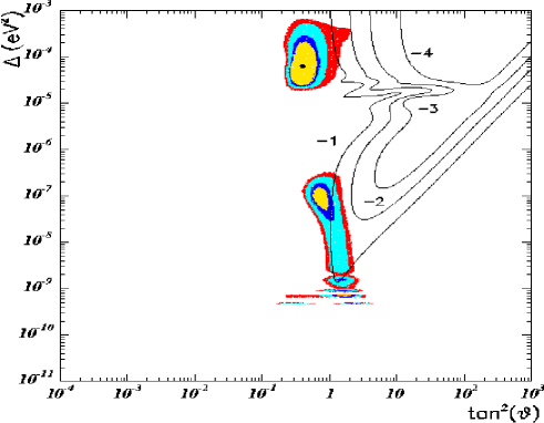
FIG. 10.: Likelihood ratio $\ln(R)$ relative to the NO–OSC hypothesis, as function of $\tan^{2}\vartheta$ and $\Delta$/eV² for $\tau=\langle E_{\bar{\nu}_{\rm h}}\rangle/\langle E_{\bar{\nu}_{\rm e}}\rangle=1.4$ (top), $\tau=1.7$ (middle) and $\tau=2$ (bottom) together with the different solutions to the solar neutrino problem. All figures for $E_{\rm b}=1.5\times 10^{53}$ erg and $\langle E_{\bar{\nu}_{\rm e}}\rangle=12$ MeV.

FIG. 11.: Likelihood ratio $\ln(R)$ relative to the NO–OSC hypothesis, as function of $\tan^{2}\vartheta$ and $\Delta$/eV² for $\tau=\langle E_{\bar{\nu}_{\rm h}}\rangle/\langle E_{\bar{\nu}_{\rm e}}\rangle=1.4$ (top), $\tau=1.7$ (middle) and $\tau=2$ (bottom) together with the different solutions to the solar neutrino problem. All figures for $E_{\rm b}=3\times 10^{53}$ erg and $\langle E_{\bar{\nu}_{\rm e}}\rangle=14$ MeV.

FIG. 12.: The 90, 95, 99 and 99.73% C.L. contours of the combined fit of solar and SN 1987A data (coloured/grey) together with the contours of the solar data alone (solid lines); for $\tau=\langle E_{\bar{\nu}_{\rm h}}\rangle/\langle E_{\bar{\nu}_{\rm e}}\rangle=1.4$ (top), $\tau=1.7$ (middle) and $\tau=2$ (bottom). All figures for $E_{\rm b}=3\times 10^{53}$ erg and $\langle E_{\bar{\nu}_{\rm e}}\rangle=14$ MeV.

FIG. 13.: The 90, 95, 99 and 99.73% C.L. contours of the combined fit of solar and SN 1987A data (coloured/grey) together with the contours of the solar data alone (solid lines); for $\tau=\langle E_{\bar{\nu}_{\rm h}}\rangle/\langle E_{\bar{\nu}_{\rm e}}\rangle=1.4$ (top), $\tau=1.7$ (middle) and $\tau=2$ (bottom). All figures for $E_{\rm b}=1.5\times 10^{53}$ erg and $\langle E_{\bar{\nu}_{\rm e}}\rangle=12$ MeV.

FIG. 14.: The 90, 95, 99 and 99.73% C.L. contours of the combined fit of solar and SN 1987A data (coloured/grey) together with the contours of the solar data alone (solid lines); for $\tau=\langle E_{\bar{\nu}_{\rm h}}\rangle/\langle E_{\bar{\nu}_{\rm e}}\rangle=1.4$ (top), $\tau=1.7$ (middle) and $\tau=2$ (bottom). All figures for $E_{\rm b}=3\times 10^{53}$ erg and $\langle E_{\bar{\nu}_{\rm e}}\rangle=16$ MeV.

FIG. 15.: The 90, 95, 99 and 99.73% C.L. contours of the combined fit of solar and SN 1987A data (coloured/grey) together with the contours of the solar data alone (solid lines); for $\tau=\langle E_{\bar{\nu}_{\rm h}}\rangle/\langle E_{\bar{\nu}_{\rm e}}\rangle=1.4$ (top), $\tau=1.7$ (middle) and $\tau=2$ (bottom). All figures for $E_{\rm b}=1\times 10^{53}$ erg and $\langle E_{\bar{\nu}_{\rm e}}\rangle=14$ MeV.

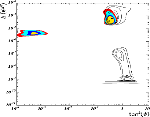
FIG. 16.: The 90, 95, 99 and 99.73% C.L. contours of the combined fit of solar and SN 1987A data (coloured/grey) together with the contours of the solar data alone (solid lines); for $\tau=\langle E_{\bar{\nu}_{\rm h}}\rangle/\langle E_{\bar{\nu}_{\rm e}}\rangle=1.4$ (top), $\tau=1.7$ (middle) and $\tau=2$ (bottom). All figures for $E_{\rm b}=3\times 10^{53}$ erg and $\langle E_{\bar{\nu}_{\rm e}}\rangle=12$ MeV.

FIG. 17.: The solid curve indicates the $\chi^{2}$ of the various oscillation solutions to the solar neutrino problem. The non-solid curves illustrate the effect of adding the SN 1987A data, which worsens the status of large mixing-type solutions. See text for explanation.

FIG. 18.: Same as in Fig. 17 but displayed with respect to $\vartheta$; see text for explanation.

Addendum: Combined analysis of SN 1987A and solar data after SNO’s NC and day/night results

In this addendum, we update our analysis including the new NC and day/night measurements of SNO [1] as well as the latest Super-K [2], SAGE [3] and GNO results [4]. As a result of the precise determination of the ⁸B flux by SNO together with the absence of spectral distortions in Super-K, the solar data disfavour now SMA-MSW, VAC, and the LOW solutions more strongly than before. To show the impact of the new measurements, we have performed a new combined $\chi^{2}$ analysis of the SN 1987A and the solar data, using the same method as described in section IV C. The $\chi^{2}_{\odot}$ were taken from Ref. [5], where also more details of this analysis can be found.

We consider again the astrophysical parameters ($E_{\rm b}$, $\langle E_{\bar{\nu}_{\rm e}}\rangle$, $\tau$ and implicitly the assumption of equipartition) as given a priori, and use only $\vartheta$ and $\Delta$ as fit parameters. Since present simulations with improved treatment of neutrino transport and microphysics (inclusion of energy transfer by recoils, nucleon bremsstrahlung, and flavour-changing neutrino annihilations $\nu_{e}\bar{\nu}_{e}\to\nu_{\mu,\tau}\bar{\nu}_{\mu,\tau}$) find much smaller differences between the spectra of $\bar{\nu}_{e}$ and $\bar{\nu}_{\mu,\tau}$, we use now only the lowest value for the ratio $\tau$ of the $\bar{\nu}_{\mu,\tau}$ and $\bar{\nu}_{e}$ temperatures considered previously, $\tau=1.4$ [6]. There are two main consequences of low $\tau$ values: First, the weight of the SN 1987A data in the combined fit is reduced. Second, deviations from equipartition which are naturally expected become more important and should not be neglected in the future.

In Fig. 19, we show the 90, 95, 99 and 99.73% C.L. contours of the combined fit for different $\bar{\nu}_{e}$ average energies, $\langle E_{\bar{\nu}_{\rm e}}\rangle=12,~{}14$ and 16 MeV. In all cases, we use $E_{\rm b}=3\times 10^{53}$ erg and $\tau=1.4$; also, we keep the assumption of equipartition to allow a simple comparison with the previous figures. The best-fit point of the combined data set lies now for all values of $\langle E_{\bar{\nu}_{\rm e}}\rangle$ in the LMA-MSW region, very close to the solar best-fit point. Both the new solar data and the small value of $\tau$ strengthen the status of LMA-MSW as the leading solution to the solar neutrino problem. Only the regions of the LMA-MSW solution with large $\Delta$ or $\tan\vartheta\mathrel{\mathop{\kern 0.0pt\hbox to0.0pt{\raise 0.86108pt\hbox{$>$}\hss}}\lower 3.87495pt\hbox{\kern-1.90002pt$\sim$}}1$ — where Earth regeneration effects are less important — are inconsistent with the combined data set. As in our previous analysis, we find that the other large mixing solutions, LOW, quasi-VAC and VAC, are disfavoured by the SN 1987A data. The LOW solution appears for small values of $\langle E_{\bar{\nu}_{\rm e}}\rangle$, but only at the 99.73% confidence level. On the other hand, the SMA-MSW solution appears at 99% C.L. if one goes to large values of $\langle E_{\bar{\nu}_{\rm e}}\rangle$.

As a concise way to illustrate these results, we show in Fig. 20 the $\chi^{2}$ in terms of only one variable, $\Delta$ or $\tan^{2}\vartheta$, respectively. The dash-dotted line is for $\tau=1.4$ and $\langle E_{\bar{\nu}_{\rm e}}\rangle=14$ MeV, the dashed line for $\tau=1.4$ and $\langle E_{\bar{\nu}_{\rm e}}\rangle=12$ MeV, while the dotted line shows $\chi^{2}$ for $\tau=1.7$ and $\langle E_{\bar{\nu}_{\rm e}}\rangle=14$ MeV. Finally, note that the arbitrary constant which appears when the maximum-likelihood analysis of SN 1987A is combined with the solar $\chi^{2}$ analysis has again been adjusted in such a way that no oscillations (and consequently the SMA-MSW solution) are unaffected by the SN 1987A data.

In summary, we find that the combined effect of current SN simulations favoring low values of $\tau$, together with the large $\chi^{2}_{\odot}$ difference between the LMA-MSW solution and its competitors, result in a very comfortable position of the LMA-MSW solution as the leading solution to the solar neutrino problem.

FIG. 19.: The 90, 95, 99 and 99.73% C.L. contours of the combined fit of solar and SN 1987A data (coloured/grey) together with the contours of the solar data alone (solid lines); for $\langle E_{\bar{\nu}_{\rm e}}\rangle=12$ MeV (top), $\langle E_{\bar{\nu}_{\rm e}}\rangle=14$ MeV (middle) and $\langle E_{\bar{\nu}_{\rm e}}\rangle=16$ MeV (bottom). All figures are for $E_{\rm b}=3\times 10^{53}$ erg and $\tau=\langle E_{\bar{\nu}_{\rm h}}\rangle/\langle E_{\bar{\nu}_{\rm e}}\rangle=1.4$.

FIG. 20.: The solid curve indicates the $\chi^{2}$ of the various oscillation solutions to the solar neutrino problem as a function of $\Delta$ (top) and $\tan^{2}\vartheta$ (bottom). The non-solid curves illustrate the effect of adding the SN 1987A data, which worsens the status of large mixing-type solutions. See text for explanation.

- [1] Q. R. Ahmad et al. [SNO Collaboration], arXiv:nucl-ex/0204008; Q. R. Ahmad et al. [SNO Collaboration], arXiv:nucl-ex/0204009.
- [2] M. B. Smy, arXiv:hep-ex/0202020.
- [3] J. N. Abdurashitov et al. [SAGE Collaboration], arXiv:astro-ph/0204245.
- [4] T. Kirsten, talk at “XXth International Conference on Neutrino Physics and Astrophysics”, Munich 2002.
- [5] P. Creminelli, G. Signorelli and A. Strumia, JHEP 0105 (2001) 052 [arXiv:hep-ph/0102234]. Version 3: addendum, discussing the implications of the NC and day/night SNO data.
- [6] G. G. Raffelt, Nucl. Phys. Proc. Suppl. 110 (2002) 254 [arXiv:hep-ph/0201099]; R. Buras, H. T. Janka, M. T. Keil, G. G. Raffelt and M. Rampp, arXiv:astro-ph/0205006; M. T. Keil, G. G. Raffelt H. T. Janka, “Monte Carlo study of supernova neutrino spectra formation” (in preparation). In the last work, values as low as have been found.