MULTIPLE PARTON RADIATION IN HADROPRODUCTION
AT LEPTON-HADRON COLLIDERS
 
By
Pavel M. Nadolsky
A THESIS
 
Submitted to
Michigan State University
in partial fulfillment of the requirements
for the degree of
 
DOCTOR OF PHILOSOPHY
 
Department of Physics & Astronomy
 
2001

ABSTRACT

MULTIPLE PARTON RADIATION IN HADROPRODUCTION
AT LEPTON-HADRON COLLIDERS
 
By
 
Pavel M. Nadolsky
 

Factorization of long- and short-distance hadronic dynamics in perturbative Quantum Chromodynamics (QCD) is often obstructed by the coherent partonic radiation, which leads to the appearance of large logarithmic terms in coefficients of the perturbative QCD series. In particular, large remainders from the cancellation of infrared singularities distort theoretical predictions for angular distributions of observed products of hadronic reactions. In several important cases, the predictive power of QCD can be restored through summation of large logarithmic terms to all orders of the perturbative expansion. Here I discuss the impact of the the coherent parton radiation on semi-inclusive production of hadrons in deep inelastic scattering at lepton-proton colliders. Such radiation can be consistently described in the $b$-space resummation formalism, which was originally developed to improve theoretical description of production of hadrons at $e^{+}e^{-}$ colliders and electroweak vector bosons at hadron-hadron colliders. I present the detailed derivation of the resummed cross section and the energy flow at the next-to-leading order of perturbative QCD. The theoretical results are compared to the experimental data measured at the $ep$ collider HERA. A good agreement is found between the theory and experiment in the region of validity of the

resummation formalism. I argue that semi-inclusive deep inelastic scattering (SIDIS) at lepton-hadron colliders offers exceptional opportunities to study coherent parton radiation, which are not available yet at colliders of other types. Specifically, SIDIS can be used to test the factorization of hard scattering and collinear contributions at small values of $x$ and to search for potential crossing symmetry relationships between the properties of the coherent radiation in SIDIS, $e^{+}e^{-}$ hadroproduction and Drell-Yan processes.

To Sunny, my true love and inspiration

ACKNOWLEDGMENTS

My appreciation goes to many people who helped me grow as a physicist. Foremost, I am deeply indebted to my advisors C.-P. Yuan and Wu-Ki Tung, who made my years at MSU a truly enriching and enjoyable experience. I feel very fortunate that C.-P. and Wu-Ki agreed to work with me when I first asked them to. Traditionally C.-P. warns each new graduate student about the challenges that accompany the career in high energy physics. In my own experience, I found that benefits and satisfaction from the work in the team with C.-P. and Wu-Ki outweigh all possible drawbacks.

Both of my advisors have spent a significant effort and time to teach me new valuable knowledge and skills. They also strongly supported my interest in the subjects of my research, both morally and through material means. I am wholeheartedly grateful for their guidance and support. The remarkable scope of vision, vigor, and patience of C.-P., together with profound knowledge, careful judgment and precision of Wu-Ki, inspire me as model personal qualities required for a scientist.

I owe my deep appreciation to my coauthor Dan Stump, who spent many focused hours working with me on the topics in this thesis. Dan’s proofreading was the main driving force behind the improvements in my English. A significant fraction of my accomplishments is due to the possibility of open and direct communication between the graduate students, MSU professors, and members of the CTEQ Collaboration. My understanding of resummation formalism was significantly enhanced through discussions with John Collins, Jianwei Qiu, Davison Soper, and George Sterman. At numerous occasions, I had useful exchanges of ideas with Edmond Berger, Raymond Brock, Joey Huston, Jim Linnemann, Fred Olness, Jon Pumplin, Wayne Repko, and Carl Schmidt. Many tasks were made easy by the interest and help from my fellow graduate students and research associates, most of all from Jim Amundson, Csaba Balazs, Qinghong Cao, Dylan Casey, Chris Glosser, Hong-Jian He, Shinya Kanemura, Stefan Kretzer, Frank Kuehnel, Liang Lai, Simona Murgia, Tom Rockwell, Tim Tait, and Alex Zhukov.

Throughout this work I was using the CTEQ Fortran libraries, which were mainly developed by W.-K. Tung, H.-L. Lai and J. Collins. The numerical package for resummation in SIDIS was developed on the basis of the programs Legacy and ResBos written by C. Balazs, G. Ladinsky and C.-P. Yuan. S. Kretzer has provided me with the Fortran parametrizations of the fragmentation functions. Some preliminary calculations included in this thesis were done by Kelly McGlynn.

I am grateful to Michael Klasen and Michael Kramer for physics discussions and invitation to give a talk at DIS2000 Workshop. I learned important information about the BFKL resummation formalism from Carl Schmidt, J. Bartels and N.P. Zotov. I thank Gunter Grindhammer and Heidi Schellman for explaining the details of SIDIS experiments at HERA and TEVATRON colliders. I also thank D. Graudenz for the correspondence about the inclusive rate of SIDIS hadroproduction, and M. Kuhlen for the communication about the HZTOOL data package. I enjoyed conversations about semi-inclusive hadroproduction with Brian Harris, Daniel Boer, Sourendu Gupta, Anna Kulesza, Tilman Plehn, Zack Sullivan, Werner Vogelsang, and other members of the HEP groups at Argonne and Brookhaven National Laboratories, University of Wisconsin and Southern Methodist University. I am grateful to Brage Golding, Joey Huston, Vladimir Zelevinsky for useful advices and careful reading of my manuscript.

I am sincerely grateful to Harry Weerts, who encouraged me to apply to the MSU graduate program and later spent a significant effort to get me in. During my years at Michigan State University, I was surrounded by the friendly and productive atmosphere created for HEP graduate students by a persistent effort of many people, notably Jeanette Dubendorf, Phil Duxbury, Stephanie Holland, Julius Kovacs, Lorie Neuman, George Perkins, Debbie Simmons, Brenda Wenzlick, Laura Winterbottom and Margaret Wilke. My teaching experience was more pleasant due to the interactions with Darlene Salman and Mark Olson.

Perhaps none of this work would be completed without the loving care and enthusiastic encouragement from my wife Sunny, who brings the meaning and joy to each day of my life. The completion of this thesis is our joint achievement, of which Sunny’s help in the preparation of the manuscript is only the smallest part. My deep gratitude also goes to my parents, who always support and love me despite my being overseas. The memory of my grandmother who passed away during the past year will always keep my heart warm.

Chapter 1 Introduction

Since its foundation in 1970’s, perturbative Quantum Chromodynamics (PQCD) has evolved into a precise theory of energetic hadronic interactions. The success of the QCD theory in the quantitative description of hadronic experimental data originates from the following fundamental ideas:

1. Hadrons are not elementary particles. As it was first shown by the quark model of Gell-Mann and Zweig [1], basic properties of the observed low-energy hadronic states are explained if hadrons are composed of a few “constituent quarks” with spin 1/2, fractional electric charges and new quantum numbers of flavor and color [2]. If the hadron constituents (partons) are bound weakly at some energy, they can possibly be detected in scattering experiments. The parton model of Feynman and Bjorken suggested that the pointlike hadronic constituents may reveal themselves in the wide-angle scattering of leptons off hadronic targets [3]. The first direct experimental proof of the hadronic substructure came from the observation of the Bjorken scaling [4] in the electron-proton deep-inelastic scattering [5]; subsequently the quantum numbers of partons were tested in a variety of experiments [6].

2. The elementary partons of QCD are “current” quarks, which interact with one another through mediation of non-Abelian gauge fields (gluons) [7]. These gauge fields are introduced to preserve the local $SU(3)$ symmetry of the quark color charges, in accordance with the pioneering work on non-Abelian gauge symmetries by C. N. Yang and R. L. Mills [8]. Remarkably, the QCD interactions weaken at small distances because of the anti-screening of color charges by self-interacting gluons [9]. Due to this feature (asymptotic freedom) of QCD, probabilities for parton interactions at distance scales smaller than $1\mbox{\, GeV}^{-1}$ can be calculated as a series in the small QCD running coupling $\alpha_{S}$. In the opposite limit of large distances, $\alpha_{S}$ grows rapidly, so that the QCD interactions become nonperturbative at the scale of about $0.2\mbox{\, GeV}^{-1}$. Such scale dependence of the QCD coupling explains why the partons behave as quasi-free particles when probed in the energetic collision, but eventually are confined in colorless hadrons at the later stages of the scattering.

3. Because of the parton confinement, quantitative calculations within QCD require systematic separation of dynamics associated with short and long distance scales. The possibility for such separation is proven by factorization theorems [10, 11, 12, 13, 14, 15]. With time, the factorization was proven for observables of increasing complexity. In 1977, G. Sterman and S. Weinberg introduced a notion of infrared-safe observables, which are not sensitive to the details of long-distance dynamics [16]. A typical example of an infrared-safe observable is the cross-section for the production of well-separated hadronic jets at an $e^{+}e^{-}$ collider. It was shown that infrared-safe observables can be systematically described by means of PQCD. As a next step, factorization was proven for inclusive observables depending on one large momentum scale $Q^{2}$. In the limit $Q^{2}\rightarrow\infty$, such observables can be factorized into a perturbatively calculable hard part, describing energetic short-range interactions of hadronic constituents, and several process-independent nonperturbative functions, relevant to the complicated strong dynamics at large distances.

The proof of factorization is more involved for hadronic observables that depend on several momentum scales (e.g., differential cross sections). The complications stem not so much from the complex dependence of the cross sections on kinematical variables, but from the presence of logarithms $\ln r$, where $r$ is some dimensionless function of the kinematical parameters of the system. For instance, $r$ may be a ratio of two momentum scales $P_{1}$ and $P_{2}$ of the system, $r=P_{1}/P_{2}$. Near the boundaries of the phase space, the ratio $r$ can be very large or very small, in which case the convergence of the series in the QCD coupling $\alpha_{S}$ can be spoiled by the largeness of terms proportional to powers of $\ln r$. Hence the factorization cannot be proven as straightforwardly as in the case of the inclusive observables, because its most obvious requirement – sufficiently rapid convergence of the perturbative series – is violated.

To restore the convergence of PQCD, one may have to sum the large logarithmic terms through all orders of $\alpha_{S}$. This procedure is commonly called resummation. Logarithmic terms of one rather general class appear due to the QCD radiation along the directions of the observed initial- or final-state hadrons (collinear radiation) or the emission of low-energy gluons (soft radiation). Such logarithms commonly affect observables sensitive to the angular distribution of the hadrons. In several important processes, the soft and collinear logarithms can be consistently resummed through the use of the formalism developed by J. Collins, D. Soper and G. Sterman (CSS).

The original resummation technique was proposed in Ref. [17] to describe angular distributions of back-to-back jets produced at $e^{+}e^{-}$ colliders (Fig. 1.1a). Subsequent developments of this technique and its comparison to the data on the $e^{+}e^{-}$ hadroproduction were presented in Refs. [18, 19, 20]. In Ref. [21] the resummation formalism   was

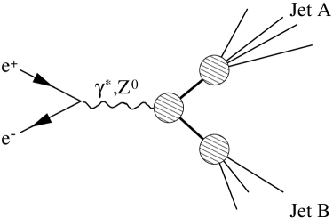
(a)

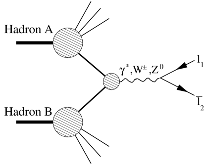
(b)

Figure 1.1: (a) Production of hadronic jets at $e^{+}e^{-}$colliders; (b) Production of lepton pairs at hadron-hadron colliders

extended to describe transverse momentum distributions of lepton pairs produced at hadron-hadron colliders (Fig. 1.1b). In the subsequent publications [22, 23, 24, 25, 26, 27], this technique was developed to a high degree of numerical accuracy. Currently the resummation analysis of this type is employed in the measurements of the mass [28] and the width [29] of the $W$-bosons produced at the $p\bar{p}$ collider TEVATRON. With some modifications, this resummation formalism is also used to improve PQCD predictions for the production of Higgs bosons [30] and photon pairs [31] at the Large Hadron Collider (LHC).

The hadroproduction at $e^{+}e^{-}$colliders and the lepton pair production at hadron-hadron colliders (Drell-Yan process) are the simplest reactions that require resummation of the soft and collinear logarithms. In both reactions, the interaction between the leptons and two initial- or final-state hadronic systems is mediated by an electroweak boson $V$ with a timelike momentum. The CSS resummation formalism can also be formulated for reactions with the exchange of a spacelike electroweak vector boson [32, 33]. In this work, I discuss resummation in the semi-inclusive production of hadrons in electron-hadron deep-inelastic scattering, which is the natural analog of $e^{+}e^{-}$ hadroproduction and Drell-Yan process in the spacelike channel. The reaction of semi-inclusive deep-inelastic scattering (SIDIS) $e+A\rightarrow e+B+X$, where $A$ and $B$ are the initial- and final-state hadrons, respectively, is shown in Figure 1.2.

As in the other two reactions, in SIDIS the multiple parton radiation affects angular distributions of the observed hadrons. The study of the resummation in SIDIS has several advantages in comparison to the reactions in the timelike channels. First, SIDIS is characterized by an obvious asymmetry between the initial and final hadronic states, so that the dependence of the multiple parton radiation on the properties of the initial state can be distinguished clearly from the dependence on the properties of the final state. In contrast, in $e^{+}e^{-}$ hadroproduction or the Drell-Yan process some details of the dynamics may be hidden due to the symmetry between two external hadronic systems. Notably, I will discuss the dependence of the resummed observables on the longitudinal variables $x$ and $z$, which can be tested in SIDIS more directly than in $e^{+}e^{-}$ hadroproduction or Drell-Yan process.

Figure 1.2: Semi-inclusive deep inelastic scattering

Second, SIDIS can be studied in the kinematical region covered by the measurements of the hadronic structure functions $F_{i}(x,Q^{2})$ in completely inclusive DIS. The ongoing DIS experiments at the $ep$ collider HERA probe $F_{i}(x,Q^{2})$ at $x$ down to $10^{-5}$, which are much smaller than lower values of $x$ reached at the existing hadron-hadron colliders. The region of low $x$, which is currently studied at HERA, will also be probed routinely in the production of $W^{\pm},Z^{0}$ and Higgs bosons at the LHC. At such low values of $x$, other dynamical mechanisms may compete with the contributions from the soft and collinear radiation described by the CSS formalism. The study of the existing SIDIS data provides a unique opportunity to learn about the applicability of the CSS formalism in the low-$x$ region and estimate robustness of theoretical predictions for the electroweak boson production at the LHC.

Last, but not the least, is the issue of potential symmetry relations between the resummed observables in SIDIS, $e^{+}e^{-}$ hadroproduction and Drell-Yan process. In SIDIS, the dynamics associated with the initial-state radiation may be similar to the initial-state dynamics in the Drell-Yan process, while the final-state dynamics may be similar to the final-state dynamics in $e^{+}e^{-}$hadroproduction. It is interesting to find out if the data support the existence of such crossing symmetry.

The results presented here were published or accepted for publication in Ref. [35, 36, 37]. The remainder of the thesis is organized as follows. In Chapter 2, I discuss the basics of factorization of mass singularities in hadronic cross sections. Then I review the general properties of the Collins-Soper-Sterman resummation formalism and illustrate some of its features with the example of hadroproduction at $e^{+}e^{-}$ colliders.

In Chapter 3, I apply the resummation formalism to semi-inclusive deep inelastic scattering. Guided by the similarities between SIDIS, $e^{+}e^{-}$ hadroproduction and Drell-Yan process, I introduce a set of kinematical variables that are particularly convenient for the identification and subsequent summation of the soft and collinear logarithms. I also identify observables that are directly sensitive to the multiple parton radiation. In particular, I argue that such radiation affects the dependence of SIDIS cross sections and hadronic energy flow on the polar angle in the photon-proton center-of-mass frame. Next I derive the ${\cal O}(\alpha_{S})$ cross section and obtain the ${\cal O}(\alpha_{S})$ coefficients for the resummed cross sections and the hadronic energy flow.

In Chapter 4, I compare the results of the CSS resummation formalism and ${\cal O}(\alpha_{S})$ fixed-order calculation with the data from the $ep$ collider HERA. I show that the CSS resummation improves theoretical description of various aspects of these data. I also discuss the dependence of the resummed observables on the longitudinal variables $x$ and $z$. I show that the HERA data are consistent with the rapid increase of nonperturbative contributions to the resummed cross section at $x\lesssim 0.01$. I discuss the potential dynamical origin of such low-$x$ behavior of the CSS formula.

Finally, in Chapter 5 I discuss the impact of the multiple parton radiation on azimuthal asymmetries of the SIDIS cross sections. I show that the CSS resummation formalism can be used to distinguish reliably between perturbative and nonperturbative contributions to the azimuthal asymmetries. I also suggest to measure azimuthal asymmetries of the transverse energy flow, which provide a clean test of PQCD.

Chapter 2 Overview of the QCD factorization

Perturbative calculations in Quantum Chromodynamics rely on a systematic procedure for separation of short- and long-distance dynamics in hadronic observables. The proof of feasibility of such procedure naturally leads to the methods for improvement of the convergence of the perturbative series when this convergence is degraded by infrared singularities of contributing subprocesses. Here I present the basics of the factorization procedure. The omitted details can be found in standard textbooks on the theory of strong interactions, e.g., Refs. [38, 39, 40, 41].

2.1 QCD Lagrangian and renormalization

Low-energy hadronic states have internal substructure. They are composed of more fundamental fermions (quarks) that are bound together by non-Abelian gauge forces. The quanta of the QCD gauge fields are called gluons. Quantum ChromoDynamics (QCD) is the theory that describes strong interactions between the quarks. In the classical field theory, the QCD Lagrangian density in the coordinate space is

$${\cal L}_{QCD}(x) = \sum_{f}\bar{\psi}_{f}\left(i{\hbox to0.0pt{/\hss}\partial}-gA_{a}\!\!\!\!\!\!/\,\,\,T_{a}-m_{f}\right)\psi_{f}$$ (2.1)

$$- \frac{1}{4}F^{\alpha\beta}_{a}F_{a\alpha\beta}-\frac{\lambda}{2}(\eta_{\alpha}A_{a}^{\alpha})^{2}+\bar{c}_{a}\left(\delta_{ad}\eta\cdot\partial-gC_{abd}\eta\cdot A_{b}\right)c_{d},$$

where $\psi_{fl}(x)$, $A^{\alpha}_{a}(x)$ and $c_{a}(x)$ are the quark, gluon and ghost fields, respectively;

$$F_{a}^{\alpha\beta}(x)\equiv\partial^{\alpha}A_{a}^{\beta}-\partial^{\beta}A^{\alpha}_{a}-gC_{abc}A_{b}^{\alpha}A^{\beta}_{c}$$ (2.2)

is the gauge field tensor; $-\lambda(\eta_{\alpha}\cdot A_{a}^{\alpha})^{2}/2$ is the term that fixes the gauge $\eta\cdot A=0$. The vector $\eta^{\alpha}$ is equal to the gradient vector $\partial^{\alpha}$ in covariant gauges $(\partial_{\alpha}A_{a}^{\alpha}=0)$ or an arbitrary vector $n^{\alpha}$ in axial gauges ($n_{\alpha}A_{a}^{\alpha}=0$). The color indices $l,m$ vary between 1 to $N_{c}$ (where $N_{c}=3$ is the number of colors), while the color indices $a,b,c,d$ vary between 1 and $N_{c}^{2}-1$. The index $f$ denotes the flavor (i.e., the type) of the quarks, which is conserved in the strong interactions. The remaining parameters in ${\cal L}_{QCD}(x)$ are the QCD charge $g$ and the masses of the quarks $m_{f}$.

The QCD Lagrangian is invariant under the gauge transformations of the $SU(N_{c})$ color group:

$$\psi_{f}(x) \rightarrow U(\theta(x))\psi_{f}(x);$$ (2.3)

$$T_{a}A_{a}^{\alpha}(x) \rightarrow U(\theta(x))T_{a}A_{a}^{\alpha}(x)U^{-1}(\theta(x))+\frac{i}{g}\left(\partial^{\alpha}U(\theta(x))\right)U^{-1}(\theta(x)),$$ (2.4)

where the $x-$dependent unitary operator $U(\theta(x))$ is

$$U(\theta(x))\equiv e^{-iT_{a}\theta_{a}(x)}.$$ (2.5)

$\left(T_{a}\right)_{lm}$ and $C_{abd}$ are generator matrices and structure constants of the color group. The commutators of the matrices $(T_{a})_{lm}$ are

$$\left[T_{a},T_{b}\right]=iC_{abc}T_{c}.$$ (2.6)

The quark fields $\psi_{fl}$ and gauge fields $A^{\alpha}_{a}$ are vectors in the fundamental and adjoint representations of $SU(N_{c})$, respectively.

In the quantum theory, $\psi_{f},\,A^{\alpha},c_{a}$ are interpreted as “bare” (unrenormalized) operators of the corresponding fields; $g$ and $m_{f}$ are interpreted as the “bare” charge and masses. The perturbative calculation introduces infinite ultraviolet corrections to these quantities. In order to obtain finite theoretical predictions, ${\cal L}_{QCD}$ has to be expressed in terms of the renormalized parameters, which are related to the “bare” parameters through infinite multiplicative renormalizations.

If the ultraviolet singularities are regularized by the continuation to $n=4-2\epsilon$, $\epsilon\nolinebreak>\nolinebreak 0$ dimensions [42], the renormalized parameters (marked by the subscript $``R^{\prime\prime}$) are related to the bare parameters as

$$\psi_{fR}(\mu) = Z_{\psi}^{-1}(\mu)\psi_{f},$$ (2.7)

$$A^{\alpha}_{aR}(\mu) = Z_{A}^{-1}(\mu)A^{\alpha}_{a},$$ (2.8)

$$c_{aR}(\mu) = Z_{c}^{-1}(\mu)c_{a},$$ (2.9)

$$g_{R}(\mu) = Z^{-1}_{g}(\mu)\mu^{-\epsilon}g,$$ (2.10)

$$m_{fR}(\mu) = Z^{-1}_{m}(\mu)m_{f},$$ (2.11)

where $Z_{\psi},Z_{A},Z_{c},Z_{g}$, and $Z_{m}$ are perturbatively calculable renormalization constants. In the dimensional regularization, the renormalized parameters depend on an auxiliary momentum scale $\mu_{n}$, which is introduced to keep the charge $g$ dimensionless in $n\neq 4$ dimensions. In Eqs. (2.7-2.11) the renormalized parameters and the constants $Z_{k}$ are expressed in terms of another scale $\mu$, which is related to $\mu_{n}$ as

$$\mu^{2}=4\pi e^{-\gamma_{E}}\mu_{n}^{2}.$$ (2.12)

Here $\gamma_{E}=0.577215...$ is the Euler constant.

2.2 Asymptotic freedom

The further improvement of the theory predictions for physical observables is achieved by enforcing their invariance under variations of the scale $\mu$, i.e., by solving renormalization group (RG) equations. Consider an observable $S$ that depends on $N$ external momenta $p_{i}^{\mu},\quad i=1,\dots,N$. If the renormalized expression for $S$ is

$$S\left(g_{R}(\mu),\{m_{fR}(\mu)\},\{p_{i}\},\mu\right)$$

(where “$\{\dots\}$” denotes a set of parameters), then the RG-improved expression for $S$ is

$$S\left(\bar{g}(\mu),\{\bar{m}_{f}(\mu)\},\{p_{i}\},\mu\right),$$ (2.13)

where $\bar{g}(\mu)$ and $\bar{m}_{f}(\mu)$ are the running QCD charge and quark masses. By solving the equation for the independence of $S$ from $\mu$,

$$\mu\frac{d}{d\mu}S\left(\bar{g}(\mu),\{\bar{m}_{f}(\mu)\},\{p_{i}\},\mu\right)=0,$$ (2.14)

we find the following differential equations for $\bar{g}(\mu)$ and $\bar{m}_{f}(\mu)$:

$$\mu\frac{\partial\bar{g}(\mu)}{\partial\mu} = \beta(\bar{g}(\mu)),$$ (2.15)

$$\mu\frac{\partial\bar{m}_{f}(\mu)}{\partial\mu} = -\gamma_{mf}\left(\bar{g}(\mu)\right)\bar{m}_{f}(\mu).$$ (2.16)

The approximate expressions for the functions $\beta(g)$ and $\gamma_{m}(g)$ on the r.h.s. of Eqs. (2.15) and (2.16) are found from the $\mu-$dependence of the fixed-order renormalized charges and masses:

$$\beta(g_{R}(\mu)) \equiv \mu\frac{\partial g_{R}(\mu)}{\partial\mu},$$ (2.17)

$$\gamma_{mf}(g_{R}(\mu)) \equiv -\frac{1}{2m_{fR}^{2}(\mu)}\mu\frac{\partial m_{fR}^{2}(\mu)}{\partial\mu}.$$ (2.18)

The renormalization group analysis of the QCD Lagrangian suggests that the interactions between the quarks weaken at high energies, i.e., that Quantum Chromodynamics is asymptotically free in this limit. Indeed, the perturbative series for the function $\beta(g)$ is

$$\beta(g)=-g\sum^{\infty}_{k=1}\left(\frac{\alpha_{S}}{4\pi}\right)^{k}\beta_{k},$$ (2.19)

where $\alpha_{S}\equiv g^{2}/4\pi$ is the QCD coupling. In the modified minimal subtraction ($\overline{MS}$) regularization scheme [43], the lowest-order coefficient $\beta_{1}$ in Eq. (2.19) is given by

$$\beta_{1} = \frac{11}{3}C_{A}-\frac{4}{3}T_{R}N_{f},$$ (2.20)

where $N_{f}$ is the number of active quark flavors, $C_{A}=N_{c}=3$, and $T_{R}=1/2$. By solving Eq. (2.15), we find that

$$\bar{\alpha}_{S}(\mu)=\frac{\bar{\alpha}_{S}(\mu_{0})}{1+\frac{\bar{\alpha}_{S}}{4\pi}\beta_{1}\ln\frac{\mu^{2}}{\mu_{0}^{2}}}.$$ (2.21)

This equation proves the asymptotic freedom of QCD interactions: for six known quark generations, $\beta_{1}>0$ and

$$\lim_{\mu\rightarrow\infty}\bar{\alpha}_{S}(\mu)=0.$$

Higher-order corrections to the beta-function do not change this asymptotic behavior. Eq. (2.21) also shows that $\bar{\alpha}_{S}(\mu)$ has a pole at some small value of $\mu$. The position of this pole can be easily found from the alternative form of Eq. (2.21),

$$\bar{\alpha}_{S}(\mu)=\frac{4\pi}{\beta_{1}\ln(\mu^{2}/\Lambda_{QCD}^{2})}\left[1+\dots\right].$$ (2.22)

In Eq. (2.22), $\Lambda_{QCD}$ is a phenomenological parameter, which is found from the analysis of the experimental data. The most recent world average value of $\Lambda_{QCD}$ for $N_{f}\nolinebreak=\nolinebreak 5$ and ${\cal O}(\alpha_{S}^{4})$ expression for the $\beta$-function is $208^{+25}_{-23}$ MeV [44]. According to Eq. (2.22), $\bar{\alpha}_{S}(\mu)$ becomes infinite when $\mu=\Lambda_{QCD}$. This feature of the QCD running coupling obstructs theoretical calculations for hadronic interactions at low energies.

2.3 Infrared safety

Due to the asymptotic freedom, the calculation of QCD observables at large $\mu$ can be organized as a series in powers of the small parameter $\bar{g}(\mu)$. To find out when the perturbative calculation may converge rapidly, consider the formal expansion of the RG-improved expression (2.13) for the observable $S$ in the series of $\bar{g}(\mu)$:

$$S=\Phi(\{p_{i}\},\{\bar{m}_{f}\},\mu)\sum^{\infty}_{k=0}S^{(k)}\left(\left\{\frac{p_{i}\cdot p_{j}}{\mu^{2}}\right\},\left\{\frac{\bar{m}_{f}(\mu)^{2}}{\mu^{2}}\right\}\right)\bar{g}^{k}(\mu).$$ (2.23)

In this expression, the function $\Phi(\{p_{i}\},\{\bar{m}_{f}\},\mu)$ includes all coefficients that do not depend on the order of the perturbative calculation (for instance, the phase space factors). The mass dimension of $\Phi(\{p_{i}\},\{\bar{m}_{f}\},\mu)$ is equal to the mass dimension of $S$. The sum over $k$ on the right-hand side is dimensionless. The coefficients of the perturbative expansion $S^{(k)}$ depend on dimensionless Lorentz-invariant combinations of the external momenta $p_{i}^{\mu}$, the mass parameter $\mu$, and the running quark masses $\bar{m}_{f}(\mu)$. There are indications that the perturbative series in Eq. (2.23) are asymptotic [45], so that it diverges at sufficiently large $k$. However, the lowest few terms of this series may approximate $S$ sufficiently well if they do not grow rapidly when $k$ increases.

The factors that control the convergence of Eq. (2.23) can be understood in a simpler case, when all Lorentz scalars $p_{i}\cdot p_{j}$ in Eq. (2.23) are of the same order $Q^{2}$. Then Eq. (2.23) simplifies to

$$S=\Phi(\{p_{i}\},\{\bar{m}_{f}\},\mu)\sum^{\infty}_{k=0}S^{(k)}\left(\frac{Q^{2}}{\mu^{2}},\left\{\frac{\bar{m}_{f}(\mu)^{2}}{\mu^{2}}\right\}\right)\bar{g}^{k}(\mu).$$ (2.24)

When $Q^{2}\gg\Lambda^{2}_{QCD}$, we can choose $\mu\sim Q$ to make $\bar{g}(\mu)$ small. This choice also eliminates potentially large terms like $\ln(Q^{2}/\mu^{2})$ from the coefficients $S^{(k)}$. In addition, let’s assume that $Q$ is much larger than any quark mass $\bar{m}_{f}(\mu)$ on which $S$ depends. For instance, $S$ may be dominated by contributions from the $u,\,d,\,s$ quarks, whose running masses are lighter than $200$ MeV at $\mu=2$ GeV [44]. At $\mu^{\prime}>2$ GeV, the quarks become even lighter due to the running of $\bar{m}_{f}$:

$$\bar{m}_{f}(\mu^{\prime})=\bar{m}_{f}(\mu)\exp\left\{-\int^{\mu^{\prime}}_{\mu}\frac{d\bar{\mu}}{\bar{\mu}}\gamma_{mf}(\bar{\mu})\right\}<\bar{m}_{f}(\mu),$$ (2.25)

since in QCD

$$\gamma_{mf}(\mu)=\frac{3\bar{\alpha}_{S}(\mu)}{4\pi}C_{F}+{\cal O}(\bar{\alpha}_{S}^{2})>0.$$ (2.26)

Here $C_{F}\equiv(N_{c}^{2}-1)/(2N_{c})=4/3$.

When the quark masses vanish, many observables, which are finite if $\bar{m}_{fi}\neq 0$, acquire infrared singularities. These singularities are generated from the terms in the perturbative coefficients that are proportional to the logarithms $\ln(\bar{m}_{f}^{2}/\mu^{2})$. The expansion in the perturbative series (2.24) makes sense only for those observables $S$ that remain finite when $\bar{m}_{f}(\mu)^{2}/\mu^{2}\rightarrow 0$.

There are two categories of observables for which the perturbative expansion (2.24) is useful. In the first case, the coefficients $S^{(k)}$ are finite and analytically calculable when $\mu\rightarrow\infty:$

$$S^{(k)}\left(\frac{Q^{2}}{\mu^{2}},\left\{\frac{\bar{m}_{f}(\mu)^{2}}{\mu^{2}}\right\}\right)\rightarrow\widetilde{S}^{(k)}\left(\frac{Q^{2}}{\mu^{2}}\right)+{\cal O}\left(\left\{\left(\frac{\bar{m}_{f}(\mu)^{2}}{\mu^{2}}\right)^{a}\right\}\right),\quad a>0.$$ (2.27)

Such observables are called infrared-safe [16]. For instance, the total and jet production cross sections in $e^{+}e^{-}$ hadroproduction are infrared-safe. In this example, hadrons appear only in the completely inclusive final state. According to the Kinoshita-Lee-Nauenberg (KLN) theorem [46], such inclusive states are free of infrared singularities, so that the finite expressions for the total and jet cross sections can be found from the massless perturbative calculation.

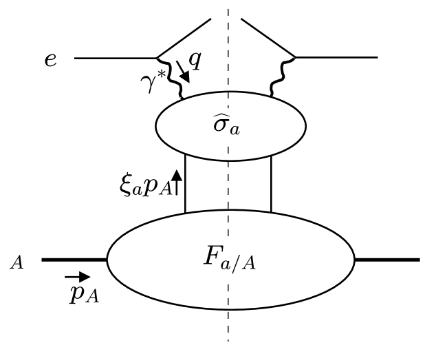
Figure 2.1: Factorization of collinear singularities in completely inclusive electron-hadron DIS

In the second case, $S^{(k)}$ are not infrared-safe, but all mass singularities of $S^{(k)}$ can be absorbed (factorized) into one or several process-independent functions. These functions can be measured in one set of experiments and then used to make predictions for other experiments.

To understand which singularities should be factorized, notice that there are two classes of the infrared singularities in a massless gauge theory: soft singularities and collinear singularities. The soft singularities occur in individual Feynman diagrams when the momentum $k^{\mu}$ carried by some gluon line vanishes ($k^{\mu}\sim\lambda\kappa^{\mu},$ where $\lambda\rightarrow 0$ and $\kappa^{\mu}$ are fixed). The soft singularities cancel at each order of $\bar{\alpha}_{S}(\mu)$ once all Feynman diagrams of this order are summed over.

In contrast, the collinear singularities occur when the momenta $p_{1}^{\mu}$ and $p_{2}^{\mu}$ of two massless particles are collinear to one another , i.e., when $p_{1}\cdot p_{2}\rightarrow 0$. Since one or both collinear particles can be simultaneously soft, the class of the collinear singularities partially overlaps with the class of the soft singularities. The soft collinear singularities cancel in the complete fixed-order result just as all soft singularities do. On the contrary, the singularities due to the collinearity of the particles with non-vanishing momenta do not cancel and should be absorbed in the long-distance phenomenological functions.

As an illustration of the factorization of the purely collinear singularities, consider the factorized form for the cross section of inclusive deep inelastic scattering $e+A\stackrel{{\scriptstyle\gamma^{*}}}{{\longrightarrow}}e+X$ (where $A$ is a hadron) in the limit $Q^{2}\rightarrow\infty$:

$$\frac{d\sigma_{A}}{dxdQ^{2}}=\sum_{a}\int^{1}_{x}d\xi_{a}\frac{d\widehat{\sigma}^{hard}_{a}}{dx\,dQ^{2}}\left(\bar{\alpha}_{S}(Q),\,\frac{x}{\xi_{a}},\,\frac{Q}{\mu_{F}}\right)F_{a/A}(\xi_{a},\mu_{F})+{\cal O}\left(\frac{1}{Q^{2}}\right).$$ (2.28)

This representation and notations for the particle momenta are illustrated in Fig. 2.1.

In Eq. (2.28), $Q^{2}\equiv-q^{2}$ is the large invariant mass of the virtual photon $\gamma^{*},$ $x\equiv Q^{2}/(2(p_{A}\cdot q))$. These variables are discussed in more detail in Subsection 3.1.1. $d\widehat{\sigma}^{hard}_{a}/\left(dx\,dQ^{2}\right)$ is the infrared-safe (“hard”) part of the cross-section for the scattering $e+a\rightarrow e+X$ of the electron on a parton $a$. $F_{a/A}(\xi_{a},\mu_{F})$ is the parton distribution function (PDF), which absorbs the collinear singularities subtracted from the full parton-level cross section to obtain $d\widehat{\sigma}^{hard}_{a}/(dx\,dQ^{2})$. In the inclusive DIS, all collinear singularities appear due to the radiation of massless partons along the direction of the initial-state hadron $A$. The final state is completely inclusive; hence, by the KLN theorem, it is finite.

The collinear radiation in the initial state depends only on the types of $a$ and $A$ and does not depend on the type of the particle reaction. Therefore, $F_{a/A}(\xi_{a},\mu_{F})$ is process-independent. It can be interpreted as a probability of finding a massless parton $a$ with the momentum $\xi_{a}p_{A}^{\mu}$ in the initial hadron with the momentum $p_{A}^{\mu}$. To obtain the complete hadron-level cross section, we sum over all possible types of $a$ ($a=g,u,\bar{u},d,\bar{d},\dots)$ and integrate over the allowed range of the momentum fractions $\xi_{a}$ $(0<x\leq\xi_{a}\leq 1)$.

In Eq. (2.28), both the “hard” cross sections $d\widehat{\sigma}^{hard}_{a}/(dx\,dQ^{2})$ and the parton distribution functions $F_{a/A}(\xi_{a},\mu_{F})$ depend on an arbitrary factorization scale $\mu_{F}$, which appears due to some freedom in the separation of the collinear contributions included in $F_{a/A}(\xi_{a},\mu_{F})$ from the “hard” contributions included in $d\widehat{\sigma}^{hard}_{a}/(dx\,dQ^{2})$. Of course, the complete hadron-level cross section on the l.h.s. of Eq. (2.28) should not depend on $\mu_{F}.$ Hence the $\mu_{F}$-dependence of $F_{a/A}(\xi_{a},\mu_{F})$ should cancel the $\mu_{F}$-dependence of the hard cross section. This requirement is used to find Dokshitser-Gribov-Lipatov-Altarelli-Parisi (DGLAP) differential equations [47], which describe the dependence of $F_{a/A}(\xi_{a},\mu_{F})$ on $\mu_{F}$:

$$\mu_{F}\frac{dF_{a/A}(\xi_{a},\mu_{F})}{d\mu_{F}}=\sum_{b}\left({\cal P}^{S}_{ab}\otimes F_{b/A}\right)(\xi_{a},\mu_{F}).$$ (2.29)

Here ${\cal P}_{ab}^{S}(\xi,\mu)$ are “spacelike” splitting functions that are currently known up to ${\cal O}(\alpha_{S}^{2})$ [48]. They describe evolution of partons with spacelike momenta. The convolution in Eq. (2.29) is defined as

$$(f\otimes g)(x,\mu)\equiv\int_{x}^{1}f(x/\xi,\mu)g(\xi,\mu)\frac{d\xi}{\xi}.$$ (2.30)

A similar approach can be used to derive factorized cross sections for reactions with observed outgoing hadrons. Such cross sections depend on fragmentation functions (FFs) $D_{B/b}(\xi,\mu_{D})$, which absorb the singularities due to the collinear radiation in the final state. The fragmentation function can be interpreted as the probability of finding the hadron $B$ among the products of fragmentation of the parton $b$. The variable $\xi$ is the fraction of the momentum of $b$ that is carried by $B$. In the presence of FFs, the hadron-level cross section becomes dependent on yet another factorization scale $\mu_{D}$. Similarly to the PDFs, the dependence of the FFs on $\mu_{D}$ is described by the DGLAP evolution equations:

$$\mu_{D}\frac{dD_{B/b}(\xi_{b},\mu_{D})}{d\mu_{D}}=\sum_{a}\left(D_{B/a}\otimes{\cal P}^{T}_{ab}\right)(\xi_{b},\mu_{D}),$$ (2.31)

where ${\cal P}_{ab}^{T}(\xi,\mu)$ are the “timelike” splitting functions.

As in the case of the renormalization scale $\mu$, it is natural to choose the factorization scales $\mu_{F}$ and $\mu_{D}$ of order $Q$ to avoid the appearance of the potentially large logarithms $\ln\left(Q/\mu_{F}\right)$ and $\ln\left(Q/\mu_{D}\right)$ in the “hard” cross section. I should emphasize that the factorized cross sections are derived under the assumption that all Lorentz scalars $p_{i}\cdot p_{j}$ are of order $Q^{2}$, so that $x$ in Eqs. (2.28) is sufficiently close to unity. When some scalar product $p_{i}\cdot p_{j}$ is much larger or smaller than $Q^{2}$, the convergence of the perturbative series for the hard cross section is worsened due to the large logarithms of the ratio $p_{i}\cdot p_{j}/Q^{2}$. This is a general observation that applies to any PQCD calculation. In some cases, the predictive power of the theory can be restored by the summation of the large logarithms through all orders of the perturbative expansion. In particular, the resummation of the large logarithms is required for the accurate description of the angular distributions of the final-state particles, including angular distributions of the final-state hadrons in SIDIS. In the next Section, I discuss general features of such resummation on the example of angular distributions of the jets in $e^{+}e^{-}$ hadroproduction.

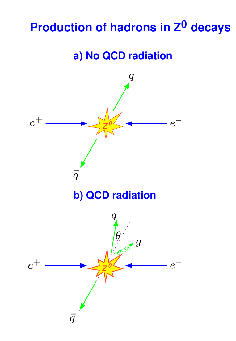
Figure 2.2: The space-time picture of hadroproduction at $e^{+}e^{-}$ colliders

2.4 Two-scale problems

2.4.1 Resummation of soft and collinear logarithms

To understand the nature of the problem, consider the process $e^{+}e^{-}\rightarrow Z^{0}\rightarrow jets$ (Fig. 1.1a). The space-time picture of this process is shown in Figure 2.2. Let us assume that the $Z^{0}$-bosons are produced at the resonance ($E_{e^{+}}+E_{e^{-}}=M_{Z}$) at rest in the laboratory frame. In $e^{+}e^{-}$ hadroproduction, the hadronic decays are initiated predominantly by the direct decay of the $Z^{0}$-boson into a quark-antiquark pair. The QCD radiation off the quarks produces hadronic jets, which are registered in the detector.

If no additional hard QCD radiation is present (Fig. 2.2a), the decay of the $Z^{0}$ boson produces two narrow jets escaping in the opposite directions in the lab frame. The typical angular width of each jet is of the order $\Lambda_{QCD}/E_{A,\,B}\ll 1$, where $E_{A,B}\approx M_{Z}/2$ are the energies of the jets. The quarks may also emit energetic gluons, in which case the angle between the jets is not equal to $\pi$ (Fig. 2.2b). If the angle $\theta$ in Fig. 2.2b is large, the additional QCD radiation is described well by the rapidly converging series in the small perturbative parameter $\alpha_{S}(M_{Z})/\pi$. But when $\theta\rightarrow 0$, the higher-order radiation is no longer suppressed, because the smallness of $\alpha_{S}(M_{Z})/\pi$ is compensated by large terms $\ln^{p}(\theta^{2}/4)/\theta^{2},\,p\geq 0$ in the hard part of the hadronic cross section. Therefore, the calculation at any fixed order does not describe reliably the shape of the hadronic cross section when $\theta\rightarrow 0$.

To illustrate this point, consider the hadronic energy-energy correlation [49], defined as

$$\frac{d\Sigma}{d\cos\theta}\equiv\frac{1}{M_{Z}^{2}}\int^{M_{Z}/2}_{0}dE_{A}\int_{0}^{M_{Z}/2}dE_{B}\,E_{A}E_{B}\frac{d\sigma}{dE_{A}dE_{B}d\cos\theta}.$$ (2.32)

In the limit $\theta\rightarrow 0$, but $\theta\neq 0$ $,d\Sigma/d\cos\theta$ behaves as

$$\left.\frac{d\Sigma}{d\cos\theta}\right|_{\theta\rightarrow 0}\approx\frac{1}{\theta^{2}}\sum^{\infty}_{k=1}\left(\frac{\alpha_{S}(M_{Z})}{\pi}\right)^{k}\,\sum_{m=0}^{2k-1}c_{km}\ln^{m}\left(\frac{\theta^{2}}{4}\right),$$ (2.33)

where $c_{km}$ are calculable dimensionless coefficients. Additionally there are virtual corrections to the lowest order cross section, which contribute at $\theta=0$. Suppose we truncate the perturbative series in Eq. (2.33) at $k=N$. If $N$ increases by 1 (that is, if we go to one higher order in the series of $\alpha_{S}$), the highest possible power of the logarithms $\ln^{m}(\theta^{2}/4)$ on the r.h.s. of Eq. (2.33) increases by 2. Therefore, the theoretical prediction does not become more accurate if the order of the perturbative calculation increases. Equivalently, the energy-energy correlation receives sizeable contributions from arbitrarily high orders of $\alpha_{S}$.

To expose the two-scale nature of this problem, let us introduce a spacelike four-vector $q_{t}^{\mu}$ and a momentum scale $q_{T}$ as

$$q_{t}^{\mu} \equiv q^{\mu}-p_{A}^{\mu}\frac{q\cdot p_{B}}{p_{A}\cdot p_{B}}-p_{B}^{\mu}\frac{q\cdot p_{A}}{p_{A}\cdot p_{B}},$$ (2.34)

$$q_{T}^{2} \equiv -q_{t}^{\mu}q_{t\mu}>0,$$ (2.35)

where $q^{\mu},\,p^{\mu}_{A},\,p_{B}^{\mu}$ are the momenta of the $Z^{0}$-boson and two jets, respectively. The vector $q_{t}^{\mu}$ is interpreted as the component of the four-momentum $q^{\mu}$ of the $Z^{0}$-boson that is transverse to the four-momenta of the jets; that is,

$$q_{t}\cdot p_{A}=q_{t}\cdot p_{B}=0.$$ (2.36)

The orthogonality of $q_{t}^{\mu}$ to both $p_{A}^{\mu}$ and $p_{B}^{\mu}$ follows immediately from its definition (2.34).

In the laboratory frame,

$$q^{\mu} = (M_{Z},\,\vec{0});$$ (2.37)

$$p_{A}^{\mu} = E_{A}(1,\,\vec{n}_{A});$$ (2.38)

$$p_{B}^{\mu} = E_{B}(1,\,-\vec{n}_{B}),$$ (2.39)

where $E_{A},\vec{n}_{A}$ and $E_{B},-\vec{n}_{B}$ are the energies of the jets and the unity vectors in the directions of the jets, respectively. The large invariant mass $q^{2}=M_{Z}^{2}$ of the $Z^{0}$-boson can be associated with the QCD renormalization scale $Q^{2}$. Let the $z$-axis be directed along $\vec{n}_{A}$. Then $q_{T}$ coincides with the length of the transverse component $\vec{q}_{T}$ of $q_{t}^{\mu}$:

$$q_{t}^{\mu}=\left(-M_{Z}\tan\frac{\theta}{2},q_{T},0,-M_{Z}\tan\frac{\theta}{2}\right).$$

At the same time

$$\frac{q_{T}^{2}}{Q^{2}}=\frac{1-\cos\theta}{1+\cos\theta},$$ (2.40)

and

$$\lim_{\theta\rightarrow 0}\frac{q_{T}^{2}}{Q^{2}}=\frac{\theta^{2}}{4}\left(1+\frac{\theta^{2}}{6}+\dots\right).$$ (2.41)

We see that the problems at $\theta\rightarrow 0$ arise due to the large logarithmic terms $\ln^{m}(q_{T}^{2}/Q^{2})/q_{T}^{2}$ when $q_{T}^{2}/Q^{2}\ll 1$:

$$\left.\frac{d\Sigma}{d\cos\theta}\right|_{\theta\rightarrow 0} \approx \frac{Q^{2}}{2}\left.\frac{d\Sigma}{dq_{T}^{2}}\right|_{q_{T}\rightarrow 0}=$$ (2.42)

$$= \frac{1}{q_{T}^{2}}\sum^{\infty}_{k=1}\left(\frac{\alpha_{S}(Q)}{\pi}\right)^{k}\,\sum_{m=0}^{2k-1}c^{\prime}_{km}\ln^{m}\left(\frac{q_{T}^{2}}{Q^{2}}\right),$$

where

$$c_{km}^{{}^{\prime}}=\frac{Q^{2}}{4}c_{km}.$$ (2.43)

The origin of these logarithms can be traced back to the presence of infrared singularities in the QCD theory. Before considering these singularities, notice that the energy-energy correlation is sufficiently inclusive to be infrared-safe. Therefore, the complete expression for the energy-energy correlation is finite at each order of $\alpha_{S}(\mu)$. On the other hand, the infrared singularities do appear in individual Feynman diagrams. According to the discussion in Section 2.3, these singularities are due to the emission of soft gluons. Although the soft singularities cancel in the sum of all Feynman diagrams at the given order of $\alpha_{S}$, this cancellation leaves large remainders $\ln^{m}(q_{T}^{2}/Q^{2})/q_{T}^{2}$ if $q_{T}$ is small.

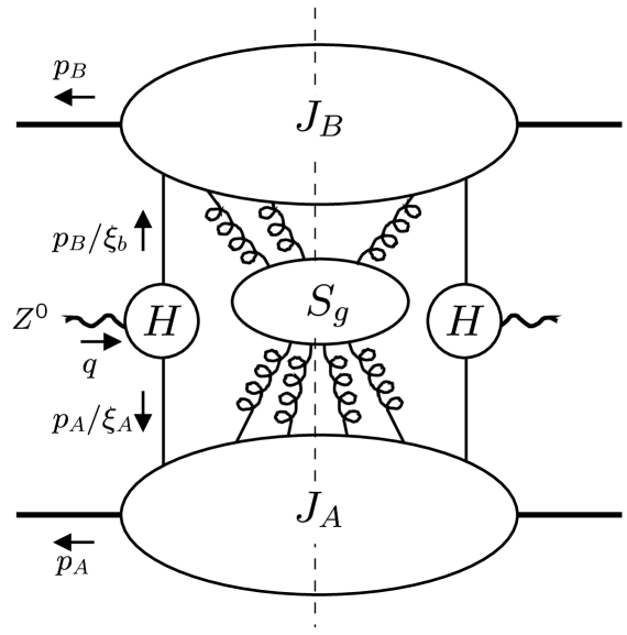
Figure 2.3: The structure of infrared singularities in a cut diagram $D$ for the energy-energy correlation in the axial gauge

Fortunately, not all coefficients $c^{\prime}_{km}$ in Eq. (2.42) are independent. Refs. [50, 51] suggested that the leading logarithmic subseries in Eq. (2.42) and in analogous expressions in SIDIS and Drell-Yan process can be summed through all orders of $\alpha_{S}$. The possibility to sum all logarithmic subseries in Eq. (2.42) and restore the convergence of the series in $\alpha_{S}$ was proven by J. Collins and D. Soper [17]. Schematically, Eq. (2.42) can be written as [23]

$$\left.\frac{d\Sigma}{dq_{T}^{2}}\right|_{q_{T}\rightarrow 0} \approx \frac{1}{q_{T}^{2}}\Bigl{\{}$$ (2.44)

$$\alpha_{S}\left(L+1\right)$$

$$+ \alpha^{2}_{S}\left(L^{3}+L^{2}+L+1\right)$$

$$+ \alpha_{S}^{3}\left(L^{5}+L^{4}+L^{3}+L^{2}+L+1\right)$$

$$+ \dots\Bigr{\}},$$

where $L\equiv\ln(q_{T}^{2}/Q^{2})$, and the coefficients $2c^{\prime}_{km}/(\pi^{k}Q^{2})$ are not shown. This series can be reorganized as

$$\left.\frac{d\Sigma}{dq_{T}^{2}}\right|_{q_{T}\rightarrow 0}\approx\frac{1}{q_{T}^{2}}\left\{\alpha_{S}Z_{1}+\alpha^{2}_{S}Z_{2}+\dots\right\},$$

where

$$\alpha_{S}Z_{1} \sim \alpha_{S}(L+1)+\alpha^{2}_{S}(L^{3}+L^{2})+\alpha^{3}_{S}(L^{5}+L^{4})+\dots\hskip 30.0pt\left|\,A_{1},B_{1},{\cal C}_{0}\right.;$$

$$\alpha^{2}_{S}Z_{2} \sim \hskip 77.0pt\alpha^{2}_{S}(L+1)+\alpha^{3}_{S}(L^{3}+L^{2})+\dots\hskip 30.0pt\left|\,A_{2},B_{2},{\cal C}_{1}\right.;$$

$$\alpha^{3}_{S}Z_{3} \sim \hskip 155.0pt\alpha^{3}_{S}(L+1)+\dots\hskip 30.0pt\left|\,A_{3},B_{3},{\cal C}_{2}\right.;$$ (2.45)

$$\dots$$

In Eq. (2.45), the right-hand side shows the new coefficients $A_{k},B_{k,}{\cal C}_{k-1}$ that are required to calculate each new subseries $\alpha^{k}_{S}Z_{k}.$ The complete subseries $\alpha_{S}^{k}Z_{k}$ can be reconstructed as soon as the coefficients $A_{k},B_{k,}{\cal C}_{k-1}$ are known from the calculation of the term $\alpha_{S}^{k}(L+1)$. Each successive subseries $\alpha_{S}^{k}Z_{k}$ in Eq. (2.45) is smaller by $\alpha_{S}$ than its predecessor, so that $\alpha_{S}$ regains its role of the small parameter of the perturbative expansion.

The rule that makes the resummation of the subseries $\alpha_{S}^{k}Z_{k}$ possible follows from (a) the analysis of the structure of the infrared singularities in the contributing Feynman diagrams at any order of $\alpha_{S}(\mu)$ and (b) the requirement that the full energy-energy correlation is infrared-safe and gauge- and renormalization-group invariant.

The structure of the infrared singularities can be identified from the analysis of analytic properties of the Feynman diagrams with the help of the Landau equations [52, 53, 54] and the infrared power counting [55, 14, 38]. This structure for some contributing cut diagram $D$ is illustrated by Figure 2.3. Throughout this discussion the axial gauge $\zeta\cdot A=0$ is used. In $D$ we can identify two jet parts $J_{A},J_{B}$, the hard vertex $H$, and possibly the soft subdiagram $S_{g}$. By their definition, the jet parts $J_{A}$ or $J_{B}$ are the connected subdiagrams of $D$ that describe the propagation of nearly on-shell massless particles inside the observed jets. Each of the particles in the jet part $J_{A}$ has a four-momentum $p_{i}^{\mu}$ that is proportional to the momentum of the jet $A$:

$$p_{i}^{\mu}=\beta_{i}p_{A}^{\mu},$$ (2.46)

where

$$0\leq\beta_{i}\leq 1,\mbox{\quad and\quad}\sum_{i}\beta_{i}=1.$$ (2.47)

Similar relations hold for the momenta of the particles in the jet part $J_{B}$.

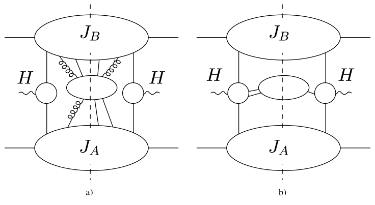
Figure 2.4: Examples of the finite soft subdiagrams: (a) the subdiagrams that are connected to $J_{A},\,J_{B}$ by one or several quark lines; (b) the subdiagrams that are connected to $H$

Both jets originate from the hard vertex $H$ that contains contributions from the highly off-shell particles. In the axial gauge the jet parts are connected to $H$ only through the single quark lines. Since the hard scattering happens practically at one point, $H$ depends only on $Q^{2}$ and not on $q_{T}^{2}$.

After the jets are created, they propagate in different directions with the speed of light. Due to the Heisenberg uncertainty principle, these jets, which are separated by large distances, do not interact with one another except by the exchange of low momentum (soft) particles. The infrared singularities, which are associated with the long-distance dynamics, can occur only in the jet parts or the soft subdiagram. This observation can be refined by the dimensional analysis of the Feynman integrals in the infrared limit [55, 14, 38], which shows that the infrared singularities are at most logarithmic. Also, those soft subdiagrams that are attached to the jet parts $J_{A}$ and $J_{B}$ with one or more quark propagators (Fig. 2.4a) or are connected to $H$ (Fig. 2.4b) are finite.

To summarize, the infrared singularities of any individual Feynman diagram reside in the soft parts of the jets $J_{A},J_{B}$ and in subdiagrams $S_{g}$ that are connected to $J_{A},\,J_{B}$ by soft gluon lines (cf. Fig. 2.3). Both types of singularities contribute at $q_{T}=0$ (i.e., $q^{\mu}=p_{A}^{\mu}+p_{B}^{\mu}$), in agreement with the expectation that the small-$q_{T}$ logarithms are remainders from the cancellation of such singularities. Therefore, at small $q_{T}$ the distribution $d\Sigma/dq_{T}^{2}$ naturally factorizes as

$$\left.\frac{d\Sigma}{dq_{T}^{2}}\right|_{q_{T}\rightarrow 0}=H(Q^{2})\,{\cal C}_{A}^{out}\,{\cal C}_{B}^{out}\,{\cal S}(q_{T}^{2},Q^{2}),$$ (2.48)

where $H(Q^{2})$ is the contribution from the pointlike hard part, ${\cal S}(q_{T}^{2},Q^{2})$ is the all-order sum of the large logarithms, and ${\cal C}_{A,B}^{out}$ collect finite contributions from the jet parts. Clearly, ${\cal C}_{A}^{out}={\cal C}_{B}^{out}$ due to the symmetry between the jets.

The factorized formula is proven by considering the Fourier-Bessel transform of $d\Sigma/dq_{T}^{2}$ to the space of the impact parameter $\vec{b}$, which is conjugate to $\vec{q}_{T}$. Explicitly,

$$\left.\frac{d\Sigma}{dq_{T}^{2}}\right|_{q_{T}\rightarrow 0}=\frac{\sigma_{0}}{S_{e^{+}e^{-}}}\int\frac{d^{2}\vec{b}}{(2\pi)^{2}}e^{i\vec{q}_{T}\cdot\vec{b}}\widetilde{W}_{\Sigma}(b,Q),$$ (2.49)

where

$$\widetilde{W_{\Sigma}}(b,Q)=\sum_{j}{\widetilde{e}}_{j}^{2}{\cal C}^{out}_{A}(C_{1},C_{2}){\cal C}^{out}_{B}(C_{1},C_{2})e^{-S(b,Q,C_{1},C_{2})}.$$ (2.50)

In Eqs. (2.49,2.50),

$$S_{e^{+}e^{-}}=Q^{2}$$ (2.51)

is the square of the center-of-mass energy of the initial-state electron and positron; $\sum_{j}$ denotes the summation over the active quark flavors (i.e., $j=u,\bar{u},d,\bar{d},\dots$); ${\widetilde{e}}_{j}$ are the couplings of the quarks to the $Z^{0}$-bosons; $(\sigma_{0}/S_{e^{+}e^{-}})\sum_{j}{\widetilde{e}}_{j}^{2}$ is the Born approximation for the hard part $H(Q^{2})$. The Fourier-Bessel transform of the shape factor ${\cal S}(q_{T}^{2},Q^{2})$ is given by $e^{-S(b,Q,C_{1},C_{2})}$, where $S(b,Q,C_{1},C_{2})$ is called the Sudakov function. At $b^{2}\ll\Lambda_{QCD}^{-2}$ (i.e., in the region of applicability of perturbative QCD), the Sudakov function is given by the integral between two momentum scales of the order $Q$ and $1/b,$ respectively:

$$\lim_{b\rightarrow 0}S(b,Q,C_{1},C_{2}) = \int_{C_{1}^{2}/b^{2}}^{C_{2}^{2}Q^{2}}\frac{d\overline{\mu}^{2}}{\overline{\mu}^{2}}\left({\cal A}(\alpha_{S}(\overline{\mu}),C_{1})\ln\frac{C_{2}^{2}Q^{2}}{\overline{\mu}^{2}}+{\cal B}(\alpha_{S}(\overline{\mu}),C_{1},C_{2})\right),$$

where ${\cal A}$ and ${\cal B}$ can be calculated in PQCD. $C_{1}$ and $C_{2}$ are arbitrary constants of the order 1 that determine the range of the integration in $S(b,Q)$. The undetermined values of these constants reflect certain freedom in separation of the collinear-soft contributions included in $S^{P}(b,Q)$ from the purely collinear contributions included in ${\cal C}$-functions. At each order of $\alpha_{S}$, changes in $S^{P}(b,Q)$ due to the variation of $C_{1},\,C_{2}$ are compensated by the opposite changes in the ${\cal C}$-functions. Hence the perturbative expansion of $\widetilde{W}_{\Sigma}$ does not depend on these constants. However, the complete form-factor $\widetilde{W}_{\Sigma}$ in Eq. (2.50) does have residual dependence on $C_{1},C_{2}$ because of the exponentiation of the terms depending on $C_{1}$ and $C_{2}$ in $\exp{(-S(b,Q,C_{1},C_{2}))}$. The variation of $C_{1},C_{2}$ allows us to test the scale invariance of the separation of soft and collinear contributions in the $\widetilde{W}_{\Sigma}$-term.

At $b^{2}\gg\Lambda_{QCD}^{-2}$, the behavior of $S$ is determined by complicated nonperturbative dynamics, which remains intractable at the current level of the development of the theory. At large $b$ the Sudakov function $S$ is parametrized by a phenomenological function $S^{NP}(b,Q)$, which has to be found from the comparison with the experimental data. When $Q\rightarrow\infty$, the sensitivity of the resummation formula to the nonperturbative part of $S(b,Q)$ is expected to decrease.

Now suppose that the experiment identifies a hadron $H_{A}$ in the jet $J_{A}$ and a hadron $B$ in the jet $J_{B}$. Let $z_{A,B}$ be the fractions of the energies of the jets $J_{A}$ and $J_{B}$ carried by $H_{A}$ and $H_{B}$, respectively. The cross section of the process $e^{+}e^{-}\stackrel{{\scriptstyle Z^{0}}}{{\longrightarrow}}H_{A}H_{B}X$ is no longer infrared-safe because of the collinear singularities due to the fragmentation into the hadrons $H_{A}$ and $H_{B}$. Nonetheless, in the limit $q_{T}\rightarrow 0$ the cross section $d\sigma/(dz_{A}dz_{B}dq_{T}^{2})$ factorizes similarly to Eqs. (2.49,2.50):

$$\left.\frac{d\sigma_{H_{A}H_{B}}}{dz_{A}dz_{B}dq_{T}^{2}}\right|_{q_{T}\rightarrow 0}=\frac{\sigma_{0}}{S_{e^{+}e^{-}}}\int\frac{d^{2}\vec{b}}{(2\pi)^{2}}e^{i\vec{q}_{T}\cdot\vec{b}}\widetilde{W}_{H_{A}H_{B}}(b,z_{A},z_{B}),$$ (2.53)

where at $b\rightarrow 0$

$$\widetilde{W}_{H_{A}H_{B}}(b,z_{A},z_{B})=\sum_{j}e_{j}^{2}\times$$

$$\left(\sum_{a}D_{H_{A}/a}\otimes{\cal C}^{out}_{aj}\right)(z_{A},b,\mu_{D})\left(\sum_{b}D_{H_{B}/b}\otimes{\cal C}^{out}_{bj}\right)(z_{B},b,\mu_{D})e^{-S};$$

$$a,b=g,\stackrel{{\scriptstyle{(-)}}}{{u}},\stackrel{{\scriptstyle{(-)}}}{{d}},\dots;$$

$$j=\stackrel{{\scriptstyle{(-)}}}{{u}},\stackrel{{\scriptstyle{(-)}}}{{d}},\dots.$$ (2.54)

The only major difference between the form-factor $\widetilde{W}_{H_{A}H_{B}}$ for the hadron pair production cross section $d\sigma/(dz_{A}dz_{B}dq_{T}^{2})$ and the form-factor $\widetilde{W}_{\Sigma}$ for the energy-energy correlation $d\Sigma/dq_{T}^{2}$ is the presence of the fragmentation functions $D_{H/a}(\xi,\mu)$, which absorb the collinear singularities due to the final-state fragmentation into the observed hadrons $H_{A},H_{B}$. The FFs are convolved with the coefficient functions ${\cal C}_{ab}^{out}(\xi,C_{1},C_{2},\mu_{D},b)$, which absorb finite contributions due to the perturbative collinear radiation.

The same resummation technique can also be applied to the production of vector bosons (e.g., virtual photons $\gamma^{*}$, which decay into lepton-antilepton pairs) at hadron-hadron colliders (Fig. 1.1b). In this process, the four-vector $q_{t}^{\mu}$ is introduced using the same definition (2.34), where now $p_{A}$ and $p_{B}$ denote the momenta of the initial hadrons $A$ and $B$. The scale $q_{T}$ is just the magnitude of the transverse momentum $p_{T}$ of $\gamma^{*}$ in the center-of-mass frame of the hadron beams (Fig. 2.5), since in this frame

$$q_{t}^{\mu}=(0,p_{T},0,0).$$

Therefore, the $b$-space resummation formalism [21] applies to the production of vector bosons with small transverse momenta. The cross section for the production of the virtual photon $\gamma^{*}$ at $q_{T}\rightarrow 0$ can be factorized as

$$\left.\frac{d\sigma_{\gamma}}{dQ^{2}dydq_{T}^{2}}\right|_{q_{T}\rightarrow 0}=\frac{\sigma^{\prime}_{0}}{S_{AB}}\int\frac{d^{2}\vec{b}}{(2\pi)^{2}}e^{i\vec{q}_{T}\cdot\vec{b}}\widetilde{W}_{\gamma}(b,x_{A},x_{B}),$$ (2.55)

where $Q^{2}$ and $y$ are the virtuality and rapidity of $\gamma^{*}$ in the lab frame, $x_{A,B}\equiv\frac{Q^{2}}{S_{AB}}e^{\pm y},$ and

$$\left.\widetilde{W}_{\gamma}(b,x_{A},x_{B})\right|_{b\rightarrow 0} = \sum_{a,b,j}e_{j}^{2}\left({\cal C}^{in}_{ja}\otimes F_{a/A}\right)(x_{A},b,\mu)\left({\cal C}^{in}_{jb}\otimes F_{b/B}\right)(x_{B},b,\mu)e^{-S}.$$

In $\widetilde{W}_{\gamma}$, $e_{j}$ are fractional electric charges of the quarks ($e_{j}=2/3$ for up quarks and $-1/3$ for the down quarks). $\left({\cal C}^{in}_{ja}\otimes F_{a/A}\right)(x_{A},b,\mu)$ and $\left({\cal C}^{in}_{jb}\otimes F_{b/B}\right)(x_{B},b,\mu)$ are the jet parts corresponding to the incoming hadrons $A$ and $B$. They are constructed from the perturbatively calculable coefficient functions ${\cal C}_{ab}^{in}(\xi,b,\mu)$ convolved with the PDFs for the relevant partons. The perturbative part of the Sudakov function in Eq. (LABEL:WV) has the same functional dependence as in Eq. (LABEL:ee_SP) for $e^{+}e^{-}$-hadroproduction. As in the case of $\widetilde{W}_{\Sigma}$ and $\widetilde{W}_{H_{A}H_{B}}$, the large-$b$ behavior of $\widetilde{W}_{\gamma}$ should be parametrized by a phenomenological function.

To conclude, the $b-$space resummation formalism was originally derived to describe the production of hadrons at $e^{+}e^{-}$ colliders [17] and production of electroweak vector bosons at hadron-hadron colliders [21]. The possibility to apply the same formalism to SIDIS relies on close similarities between the three processes. First, hadronic interactions in all three processes are described by the same set of Feynman diagrams in different crossing channels. Second, multiple parton radiation dominates each of the three processes when the final-state particle escapes closely to the direction predicted by the leading-order kinematics. The formalism for the resummation of such radiation can be formulated in Lorentz-invariant notations, so that it can be continued from one process to another.

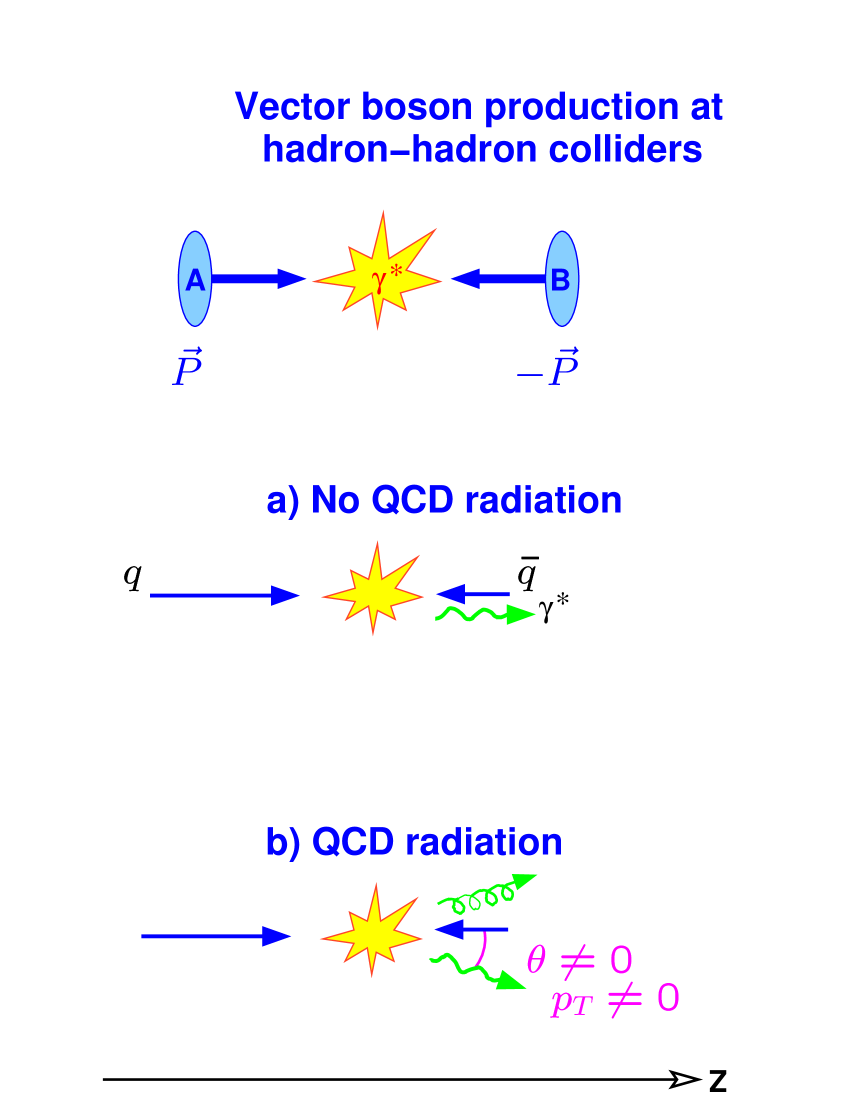
Figure 2.5: The space-time picture of Drell-Yan process

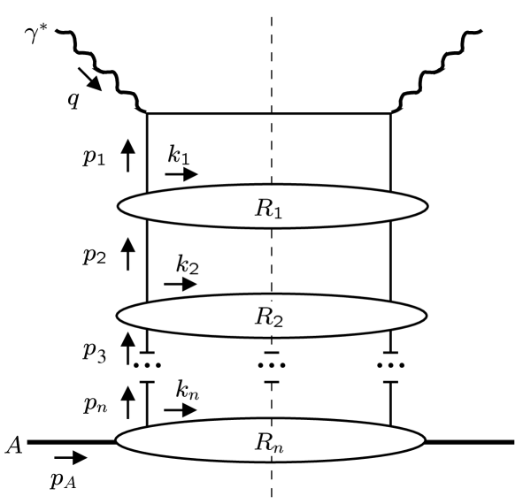
Figure 2.6: The ladder structure of the DIS cut diagrams

2.4.2 QCD at small $x$

According to the discussion in Section 2.3, the convergence of the series in $\alpha_{S}(\mu)$ depends on the absence of very large or small dimensionless quantities in the perturbative coefficients. In particular, the dimensionless variable $x$ in the inclusive DIS cross section should not be too close to zero: otherwise the hard part of the DIS cross section contains large logarithms $\ln^{m}(1/x)$, which compensate for the smallness of $\alpha_{S}(Q)$. These logarithms are different from the logarithms $\ln^{m}\mu^{2}$ resummed by the DGLAP evolution equations. As a result, the factorization of the DIS cross section in the hard cross section and PDFs (cf. Eq. (2.28)) may experience difficulties at small $x$.

The large logarithms $\ln^{m}(1/x)$ are resummed in the formalism of Balitsky, Fadin, Kuraev and Lipatov (BFKL) [56]. The BFKL and DGLAP pictures for the history of the parton probed in the hard scattering are quite different. Both types of formalisms resum contributions from the cut ladder diagrams shown in Figure 2.6. In this Figure, each “rung” $R_{k}$ is a two-particle irreducible subdiagram that corresponds to the radiation off the probed parton line (see Refs. [38, 57] for more details). The vertical propagators correspond to the quarks or the gluons that are parents to the probed quark. The momenta $p_{1,2,\dots,n}^{\mu}$ flow from the parent hadron to the probed quark. The momenta $k_{1,2,\dots,n}^{\mu}$ flow through the rungs and are sums of the momenta of the radiated particles. The conservation of the momentum in each rung implies that

$$p_{i}^{\mu}=p_{i+1}^{\mu}-k_{i}^{\mu},\quad\quad i=1,\dots,n,$$ (2.57)

where $p_{n+1}^{\mu}\equiv p_{A}^{\mu}$. In the reference frame where the hadron $A$ moves at the speed of light along the $z$-axis, $x$ coincides with the ratio of the plus components of $p_{0}^{\mu}$ and $p_{A}^{\mu}$:

$$x=\frac{p_{0}^{+}}{p_{A}^{+}},$$ (2.58)

where

$$k^{\pm}\equiv k^{0}\pm k^{3}.$$ (2.59)

The DGLAP equation arises from the resummation of the ladder diagrams corresponding to the collinear radiation along the direction of the hadron $A$. The radiating parton remains highly boosted at each rung of the ladder. At the same time, the transverse momentum carried away by the radiation grows rapidly from the bottom to the top of the ladder. The DGLAP equation corresponds to the strong ordering of the transverse momenta flowing through the rungs $R_{i}$: that is,

$$Q^{2}\gg k^{2}_{T1}\gg k^{2}_{T2}\gg\dots\gg k^{2}_{Tn}\gg\Lambda_{QCD}^{2},$$ (2.60)

while

$$p_{1}^{+}\sim p_{2}^{+}\sim\dots\sim p_{n}^{+}\sim p_{A}^{+}\gg 0$$ (2.61)

and

$$p_{1}^{-}\sim p_{2}^{-}\sim\dots\sim p_{n}^{-}\sim p_{A}^{-}\sim 0.$$ (2.62)

On the other hand, the BFKL formalism describes the situation in which the QCD radiation carries away practically all energy of the probed parton. In this case,

$$p_{1}^{+}\ll p_{2}^{+}\ll\dots\ll p_{n}^{+}\ll p_{A}^{+},$$ (2.63)

and

$$p_{1}^{-}\gg p_{2}^{-}\gg\dots\gg p_{n}^{-}\gg p_{A}^{-}.$$ (2.64)

In addition, the BFKL picture imposes no ordering on the transverse components of $k_{i}^{\mu}$:

$$k_{T1}^{2}\sim k_{T2}^{2}\sim\dots\sim k_{Tn}^{2}\gg\Lambda^{2}_{QCD}.$$ (2.65)

As a result, the probed quark is likely to have a significant transverse momentum throughout the whole process of evolution, which is impossible in the DGLAP picture. Due to its large $k_{T}$, the radiating parton is off its mass shell at any moment of its evolution history, so that the BFKL radiation cannot be factorized from the hard scattering. As another consequence of the $k_{T}$-unordered radiation, the BFKL picture implies broad angular distributions of the final-state hadrons, while in the DGLAP picture the hadrons are more likely to belong to the initial- and final-state jets.

Since the BFKL approach applies to the limit $x\rightarrow 0$ and $k_{iT}^{2}\gg\Lambda_{QCD}^{2}$, it corresponds to asymptotically high energies of hadronic collisions. So far, the experiments have produced no data that would definitely require the BFKL formalism to explain them. In particular, the behavior of the inclusive DIS structure functions in the low $x$ region at HERA agrees well with the ${\cal O}(\alpha_{S}^{2})$ predictions of the traditional factorized formalism and disagrees with the steep power-law growth predicted by the leading-order solution of the BFKL equation [56].

The situation is not so clear for some less inclusive observables, which deviate from the low-order predictions of PQCD. Specifically, SIDIS in the small-$x$ region is characterized by large higher-order corrections. Some of these corrections can be potentially attributed to the enhanced $k_{T}$-unordered radiation at $x\rightarrow 0$. If this is indeed the case, the effects of the $k_{T}$-unordered radiation may be identified by observing the changes in the angular distributions of the final-state hadrons or “intrinsic $k_{T}$” of the partons. In order to pinpoint these effects, good understanding of the angular dynamics in the traditional DGLAP picture is needed. Such understanding can be achieved in the framework of the small-$q_{T}$ resummation formalism, which systematically describes angular distributions of the hard, soft and collinear radiation. Hence it can be naturally used to organize our knowledge about the angular patterns of the DGLAP radiation and search for the effects from new low-$x$ QCD dynamics.

Chapter 3 Resummation in semi-inclusive DIS: theoretical formalism

Deep-inelastic lepton-hadron scattering (DIS) is one of the cornerstone processes to test PQCD. Traditionally, the experimental study of the fully inclusive DIS process $e+A\rightarrow e+X$, where $A$ is usually a nucleon, and $X$ is any final state, is used to measure the parton distribution functions (PDFs) for $A$. These functions describe the long-range dynamics of hadron interactions and are required by many PQCD calculations. During the 1990’s, significant attention has been also paid to various aspects of semi-inclusive deep inelastic scattering (SIDIS), for instance, the semi-inclusive production of hadrons and jets, $e+A\rightarrow e+B+X$ and $e+A\rightarrow e+jets+X$. In particular, the H1 and ZEUS collaborations at HERA, European Muon Collaboration at CERN, and the E665 experiment at Fermi National Accelerator Laboratory performed extensive experimental studies of the charged particle multiplicity [58, 59, 60, 61, 62, 63] and hadronic transverse energy flows [64, 65] at large momentum transfer $Q$. It was found that some aspects of the data, e.g., the Feynman $x$ distributions, can be successfully explained in the framework of PQCD analysis [66, 67]. On the other hand, applicability of PQCD to the description of other features of the process is limited. For example, the perturbative calculation in lowest orders fails to describe the pseudorapidity or transverse momentum distributions of the final hadrons. Under certain kinematical conditions the whole perturbative expansion as a series in the QCD coupling may fail due to the large logarithms discussed in Section 2.4.

To be more specific, consider semi-inclusive DIS production of hadrons of a type $B$. At large energies, one can neglect the masses of the participating particles. In semi-inclusive DIS at given energies of the beams, any event can be characterized by two energy scales: the virtuality of the exchanged vector boson $Q$ and the scale $q_{T}$ introduced analogously to $e^{+}e^{-}$ hadroproduction and Drell-Yan process (cf. Section 2.4). The scale $q_{T}$ is also related to the transverse momentum of $B$. The expansion in the series of $\alpha_{S}$ is justified if at least one of these scales is much larger than $\Lambda_{QCD}$. However, the above necessary condition does not guarantee fast convergence of perturbative series in the presence of large logarithmic terms. If $\Lambda^{2}_{QCD}\ll Q^{2},\,q^{2}_{T}\ll Q^{2}$, the cross sections are dominated by the soft and collinear logarithms $\log^{m}\left(q^{2}_{T}/Q^{2}\right),$ which can be resummed in the framework of the small-$q_{T}$ resummation formalism (Subsection 2.4.1). In the limit $\Lambda^{2}_{QCD}\ll q^{2}_{T},\,Q^{2}\ll q^{2}_{T}$ (photoproduction region) PQCD may fail due to the large terms $\log^{m}\left(Q^{2}/q^{2}_{T}\right)$, which should be resummed into the parton distribution function of the virtual photon [68]. Finally, even in the region $\Lambda^{2}_{QCD}\ll q^{2}_{T}\sim Q^{2}$ one may encounter another type of large logarithms corresponding to events with large rapidity separation between the partons and/or the hadrons. This type of large logarithms can be resummed with the help of the Balitsky-Fadin-Kuraev-Lipatov (BFKL) formalism (Subsection 2.4.2).

In this Chapter I discuss resummation of soft and collinear logarithms in SIDIS hadroproduction $e+A\rightarrow e+B+X$ in the limit $\Lambda_{QCD}^{2}\ll Q^{2},\,q_{T}^{2}\ll Q^{2}$. The calculations are based on the works by Meng, Olness, and Soper [34, 33], who analyzed the resummation technique for a particular energy distribution function of the SIDIS process. This energy distribution function receives contributions from all possible final-state hadrons and does not depend on the specifics of fragmentation.

Here the resummation is discussed in a more general context compared to [34, 33]: namely, I also consider the final-state fragmentation of the partons. Using this formalism, I discuss the impact of soft and collinear PQCD radiation on a wide class of physical observables including particle multiplicities. The calculations will be done in the next-to-leading order of PQCD. In the next Chapter, I compare the resummation formalism with the H1 data on the pseudorapidity distributions of the transverse energy flow [64, 65] and ZEUS data on multiplicity of charged particles [60] in the $\gamma^{*}p$ center-of-mass frame. Another goal of this study is to find in which regions of kinematical parameters the CSS resummation formalism is sufficient to describe the existing data, and in which regions significant contributions from other hadroproduction mechanisms, such as the BFKL radiation [56], higher-order corrections including multijet production with [68] or without [69, 70] resolved photon contributions, or photoproduction showering [71], cannot be ignored.

3.1 Kinematical Variables

I follow notations which are similar to the ones used in [34, 33]. In this Section I summarize them.

I consider the process

$$e+A\rightarrow e+B+X,$$ (3.1)

where $e$ is an electron or positron, $A$ is a proton (or other hadron in the initial state), $B$ is a hadron observed in the final state, and $X$ represents any other particles in the final state in the sense of inclusive scattering (Fig. 1.2). I denote the momenta of $A$ and $B$ by $p_{A}^{\mu}$ and $p_{B}^{\mu}$, and the momenta of the electron in the initial and final states by $l^{\mu}$ and $l^{\prime\mu}$. Also, $q^{\mu}$ is the momentum transfer to the hadron system, $q^{\mu}=l^{\mu}-l^{\prime\mu}$. Throughout all discussion, I neglect particle masses.

I assume that the initial electron and hadron interact only through a single photon exchange. Contributions due to the exchange of $Z$-bosons or higher-order electroweak radiative corrections will be neglected. Therefore, $q^{\mu}$ also has the meaning of the 4-momentum of the exchanged virtual photon $\gamma^{*}$; $q^{\mu}$ is completely determined by the momenta of the initial- and final-state electrons. In many respects, DIS behaves as scattering of virtual photons on hadrons, so that the theoretical discussion of hadronic interactions can often be simplified by considering only the photon-proton system.

3.1.1 Lorentz scalars

For further discussion, I define five Lorentz scalars relevant to the process (3.1). The first is the center-of-mass energy of the initial hadron and electron $\sqrt{S_{eA}}$ where

$$S_{eA}\equiv(p_{A}+l)^{2}=2p_{A}\cdot l.$$ (3.2)

I also use the conventional DIS variables $x$ and $Q^{2}$ which are defined from the momentum transfer $q^{\mu}$ by

$$Q^{2}\equiv-q^{2}=2\ell\cdot\ell^{\prime},$$ (3.3)

$$x\equiv\frac{Q^{2}}{2p_{A}\cdot q}.$$ (3.4)

In principle, $x$ and $Q^{2}$ can be completely determined in an experimental event by measuring the momentum of the outgoing electron.

Next I define a scalar $z$ related to the momentum of the final hadron state $B$ by

$$z=\frac{p_{B}\cdot p_{A}}{q\cdot p_{A}}=\frac{2xp_{B}\cdot p_{A}}{Q^{2}}.$$ (3.5)

The variable $z$ plays an important role in the description of fragmentation in the final state. In particular, in the quark-parton model (or in the leading order perturbative calculation) it is equal to the fraction of the fragmenting parton’s momentum carried away by the observed hadron.

The next relativistic invariant $q_{T}^{2}$ is the square of the component of the virtual photon’s 4-momentum $q^{\mu}$ that is transverse to the 4-momenta of the initial and final hadrons:

$$q_{T}^{2}=-q_{t}^{\mu}q_{t\mu},$$ (3.6)

where

$$q_{t}^{\mu}=q^{\mu}-p_{A}^{\mu}\frac{q\cdot p_{B}}{p_{A}\cdot p_{B}}-p_{B}^{\mu}\frac{q\cdot p_{A}}{p_{A}\cdot p_{B}}.$$ (3.7)

As discussed in Subsection 2.4.1, the momentum $q_{t}^{\mu}$ plays the crucial role in the resummation of the soft and collinear logarithms. In particular, a fixed-order PQCD cross-section is divergent when $q_{T}\rightarrow 0$, so that all-order resummation is needed to make the theory predictions finite in this limit. According to Eqs. (3.5,3.7) $q_{t}^{\mu}=0$ if and only if $p_{B}^{\mu}=z\left(xp_{A}^{\mu}+q^{\mu}\right).$ Hence the resummation is required when the final-state hadron $B$ approximately follows the direction of $x\vec{p}_{A}+\vec{q}.$

In the analysis of kinematics, I will use three reference frames. The most obvious frame is the laboratory frame, or the rest frame of the experimental detector. The observables in this frame are measured directly, but the theoretical analysis is complicated due to the varying momentum of the photon-proton system. Hence I will mostly use two other reference frames, the center-of-mass frame of the initial hadron and the virtual photon (hadronic c.m., or hCM frame), and a special type of Breit frame which I will call, depending on whether the initial state is a hadron or a parton, the hadron or parton frame. As was shown in Ref. [33], the resummed cross section can be derived naturally in the hadron frame. On the other hand, many experimental results are presented for observables in the hCM frame. These observables are not measured directly; rather they are reconstructed from directly measured observables in the laboratory frame. I will use subscripts $h$, $cm$ and $lab$ to denote kinematical variables in the hadron, hCM or laboratory frame. Below I discuss kinematical variables in all three frames.

3.1.2 Hadron frame

Following Meng et al. [34, 33] the hadron frame is defined by two conditions: (a) the energy component of the 4-momentum of the virtual photon is zero, and (b) the momentum of the outgoing hadron $B$ lies in the $xz$ plane. The directions of particle momenta in this frame are shown in Fig. 3.1.

In this frame the proton $A$ moves in the $+z$ direction, while the momentum transfer $\vec{q}$ is in the $-z$ direction, and $q^{0}$ is 0:

$$q^{\mu}_{h} = \left(0,0,0,-Q\right),$$ (3.8)

$$p_{A,h}^{\mu} = \frac{Q}{2x}\left(1,0,0,1\right).$$ (3.9)

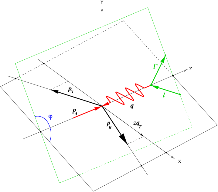
Figure 3.1: Geometry of the particle momenta in the hadron frame

The momentum of the final-state hadron $B$ is

$$p_{B,h}^{\mu}=\frac{zQ}{2}\Bigl{(}1+\frac{q_{T}^{2}}{Q^{2}},\frac{2q_{T}}{Q},0,\frac{q_{T}^{2}}{Q^{2}}-1\Bigr{)}.$$ (3.10)

The incoming and outgoing electron momenta in the hadron frame are defined in terms of variables $\psi$ and $\varphi$ as follows [83]:

$$\ell^{\mu}_{h} = \frac{Q}{2}\left(\cosh\psi,\sinh\psi\cos\varphi,\sinh\psi\sin\varphi,-1\right),$$

$$\ell^{\prime\mu}_{h} = \frac{Q}{2}\left(\cosh\psi,\sinh\psi\cos\varphi,\sinh\psi\sin\varphi,+1\right).$$ (3.11)

Note that $\varphi$ is the azimuthal angle of $\vec{\ell}_{h}$ or $\vec{\ell}^{\prime}_{h}$ around the $Oz$-axis. $\psi$ is a parameter of a boost which relates the hadron frame to an electron Breit frame in which $\ell^{\mu}=(Q/2,0,0,-Q/2)$. By (3.2) and (3.11)

$$\cosh\psi=\frac{2xS_{eA}}{Q^{2}}-1=\frac{2}{y}-1,$$ (3.12)

where the conventional DIS variable $y$ is defined as

$$y\equiv\frac{Q^{2}}{xS_{eA}}.$$ (3.13)

The allowed range of the variable $y$ in deep-inelastic scattering is $0\leq y\leq 1$ (see Subsection 3.1.4); therefore $\psi\geq 0$.

The transverse part of the virtual photon momentum $q_{t}^{\mu}$ has a simple form in the hadron frame; it can be shown that

$$q_{t,h}^{\mu}=(-\frac{q_{T}^{2}}{Q},-q_{T},0,-\frac{q_{T}^{2}}{Q}).$$ (3.14)

In other words, $q_{T}$ is the magnitude of the transverse component of $\vec{q}_{t,h}$. The transverse momentum $p_{T}$ of the final-state hadron $B$ in this frame is simply related to $q_{T}$, by

$$p_{T}=zq_{T}.$$ (3.15)

Also, the pseudorapidity of $B$ in the hadron frame is

$$\eta_{h}\equiv-\log\Bigl{(}\tan\frac{\theta_{B,h}}{2}\Bigr{)}=\log\frac{q_{T}}{Q}.$$ (3.16)

The resummed cross-section will be derived using the hadron frame. To transform the result to other frames, it is useful to express the basis vectors of the hadron frame ($T^{\mu},\,\,X^{\mu},\,\,Y^{\mu},Z^{\mu}$) in terms of the particle momenta [34]. For an arbitrary coordinate frame,

$$T^{\mu} = \frac{q^{\mu}+2xp_{A}^{\mu}}{Q},$$

$$X^{\mu} = \frac{1}{q_{T}}\Biggl{(}\frac{p^{\mu}_{B}}{z}-q^{\mu}-\Bigl{[}1+\frac{q_{T}^{2}}{Q^{2}}\Bigr{]}xp_{A}^{\mu}\Biggr{)},$$

$$Y^{\mu} = \epsilon^{\mu\nu\rho\sigma}Z_{\nu}T_{\rho}X_{\sigma},$$

$$Z^{\mu} = -\frac{q^{\mu}}{Q}.$$ (3.17)

If these relations are evaluated in the hadron frame, the basis vectors $T^{\mu},\,\,X^{\mu},\,\,Y^{\mu},Z^{\mu}$ are $(1,0,0,0),\,\,(0,1,0,0),(0,0,1,0),(0,0,0,1)$, respectively.

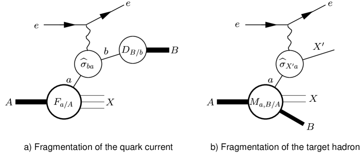
Figure 3.2: (a) In the current fragmentation region, the hadron-level cross section can be factorized into hard partonic cross sections $\widehat{\sigma}_{ba}$, parton distribution functions $F_{a/A}(\xi_{a},\mu_{F})$, and fragmentation functions $D_{B/b}(\xi_{b},\mu_{F})$. (b) In the target fragmentation region, the hadrons are produced through the mechanism of diffractive scattering that depends on “diffractive parton distributions” $M_{a,B/A}(\xi_{a},\zeta_{B},\mu_{F}).$

The limit of small $q_{T}$, which is the most relevant for our resummation calculation, corresponds to the region of large negative pseudorapidities in the hadron frame. Hence the resummation affects the rate of the production of the hadrons that follow closely the direction of the virtual photon. The region of negative $\eta_{h}$ is often called the current fragmentation region, since the final-state hadrons are produced due to the interaction of the virtual photon with the quark current. In the current fragmentation region, hadroproduction proceeds through independent scattering and subsequent fragmentation of partons. Therefore, in this region the hadron-level cross section $\sigma_{BA}$ can be factorized in the cross sections $\widehat{\sigma}_{ba}$ for the electron-parton scattering $e+a\rightarrow e+b+X$, the PDFs $F_{a/A}(\xi_{a},\mu_{F})$, and the FFs $D_{B/b}(\xi_{b},\mu_{D})$ (cf. Figure 3.2a). The formal proof of the factorization in the current region of SIDIS can be found in [32, 72].

In the opposite direction $\eta_{h}\gg 0$ ($q_{T}\rightarrow+\infty$) contributions from the current fragmentation vanish. Rather the produced hadron is likely to be a product of fragmentation of the target proton, which moves in the $+z$-direction (cf. Eq. (3.9)). According to Eq. (3.5), such hadrons have $z\approx 0$. The target fragmentation hadroproduction is described by a different approach, which relies on factorization of the hadron-level cross section into cross sections of parton subprocesses and diffractive parton distributions $M_{a,B/A}(\xi_{a},\zeta_{B},\mu_{F})$ (cf. Figure 3.2b). These distributions can be interpreted as probabilities for the initial hadron $A$ to fragment into the parton $a$, the hadron $B$, and anything else. $\xi_{a}$ and $\zeta_{B}$ denote fractions of the momentum of $A$ that are carried by the parton $a$ and the hadron $B$, respectively. The distributions $M_{a,B/A}(\xi_{a},\zeta_{B},\mu_{F})$ (also called fracture functions) were introduced in Refs. [73, 74] and used in [67, 75, 76, 77] to describe various aspects of SIDIS with unpolarized and polarized beams. The factorization of cross sections in the target fragmentation region was formally proven in the scalar field theory [78] and in full QCD [79, 80]. The recent experimental studies of the diffractive scattering at HERA are reviewed in [81]. The detailed discussion of diffractive scattering and interesting models [82] that are applied for its analysis is beyond the scope of this work.

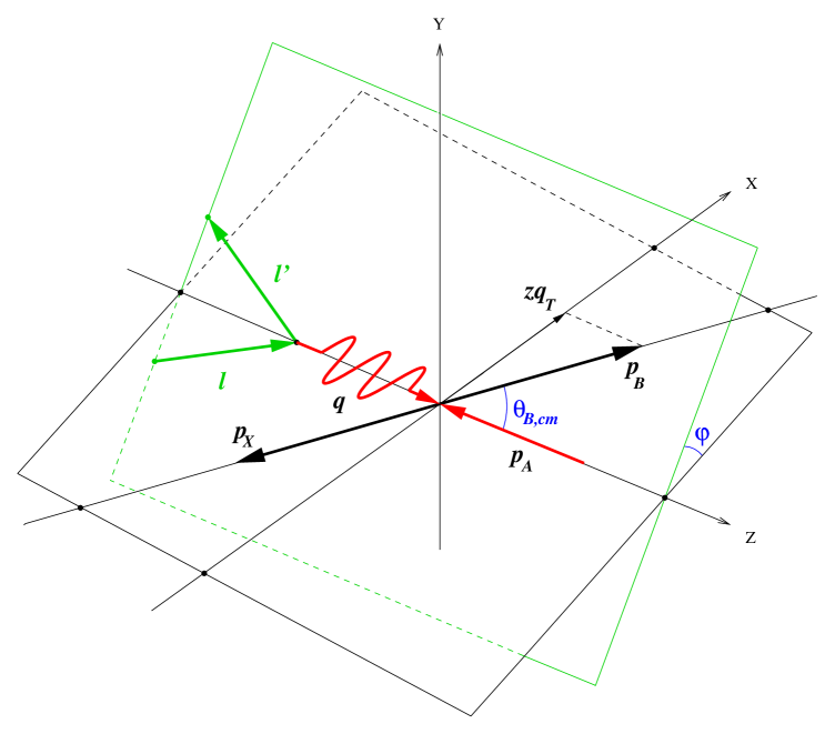
Figure 3.3: Particle momenta in the hadronic center-of-mass (hCM) frame

3.1.3 Photon-hadron center-of-mass frame

The center-of-mass frame of the proton $A$ and virtual photon $\gamma^{*}$ is defined by the condition $\vec{p}_{A,cm}+\vec{q}_{cm}=0$. The relationship between particle momenta in this frame is illustrated in Fig. 3.3. As in the hadron frame, the momenta $\vec{q}_{cm}$ and $\vec{p}_{A,cm}$ in the hCM frame are directed along the $Oz$ axis. The coordinate transformation from the hadron frame into the hCM frame consists of (a) a boost in the direction of the virtual photon and (b) inversion of the direction of the $Oz$ axis, which is needed to make the definition of the hCM frame consistent with the one adopted in HERA experimental publications. In the hCM frame the momentum of $\gamma^{*}$ is

$$q_{cm}^{\mu}=\Biggl{(}\frac{W^{2}-Q^{2}}{2W},0,0,\frac{W^{2}+Q^{2}}{2W}\Biggr{)},$$ (3.18)

where $W$ is the hCM energy of the $\gamma^{*}p$ collisions,

$$W^{2}\equiv(p_{A}+q)^{2}=Q^{2}\left(\frac{1}{x}-1\right)\geq 0.$$ (3.19)

Since all energy of the $\gamma^{*}p$ system is transformed into the energy of the final-state hadrons, $W$ coincides with the invariant mass of the $B+X$ system.

The momenta of the initial and final hadrons $A$ and $B$ are given by

$$p^{\mu}_{A,cm}=\Biggl{(}\frac{W^{2}+Q^{2}}{2W},0,0,-\frac{W^{2}+Q^{2}}{2W}\Biggr{)},$$ (3.20)

$$p^{\mu}_{B,cm}=\Biggl{(}E_{B},E_{B}\sin\theta_{B,cm},0,E_{B}\cos\theta_{B,cm}\Biggr{)},$$ (3.21)

where

$$E_{B} = z\frac{W^{2}+q_{T}^{2}}{2W},$$ (3.22)

$$\cos\theta_{B,cm} = \frac{W^{2}-q_{T}^{2}}{W^{2}+q_{T}^{2}}.$$ (3.23)

The hadron and hCM frames are related by a boost along the $z$-direction, so that the expression for the transverse momentum of the final hadron $B$ in the hCM frame is the same as the one in the hadron frame,

$$p_{T}=zq_{T}.$$ (3.24)

Also, similar to the case of the hadron frame, the relationship between $q_{T}$ and the pseudorapidity of $B$ in the hCM frame is simple,

$$q_{T}=We^{-\eta_{cm}}.$$ (3.25)

Since the directions of the $z$-axis are opposite in the hadron frame and the hCM frame, large negative pseudorapidities in the hadron frame ($q_{T}\rightarrow 0$) correspond to large positive pseudorapidities in the hCM frame. Hence multiple parton radiation effects should be looked for in SIDIS data at $q_{T}/Q\lesssim 1$, or

$$\eta_{cm}\gtrsim\ln\left(\sqrt{\frac{1-x}{x}}\right)>2.$$ (3.26)

The boost from the hadron to the hCM frame also preserves the angle $\varphi$ between the planes of the hadronic and leptonic momenta, so that the momenta $l^{\mu},l^{\prime\mu}$ of the electrons in the hCM frame are

$$l_{cm}^{\mu}=\Biggl{\{}\frac{1}{4W}\biggl{(}(W^{2}+Q^{2})\cosh\psi+W^{2}-Q^{2}\biggr{)},\frac{Q}{2}\sinh\psi\cos\varphi,$$

$$-\frac{Q}{2}\sinh\psi\sin\varphi,\frac{1}{4W}\biggl{(}(W^{2}+Q^{2})+(W^{2}-Q^{2})\cosh\psi\biggr{)}\Biggr{\}};$$ (3.27)

$$l_{cm}^{\prime\mu}=\Biggl{\{}\frac{1}{4W}\biggl{(}(W^{2}+Q^{2})\cosh\psi-W^{2}+Q^{2}\biggr{)},\frac{Q}{2}\sinh\psi\cos\varphi,$$

$$-\frac{Q}{2}\sinh\psi\sin\varphi,\frac{1}{4W}\biggl{(}-W^{2}-Q^{2}+(W^{2}-Q^{2})\cosh\psi\biggr{)}\Biggr{\}}.$$ (3.28)

Finally I would like to mention two more variables, which are commonly used in the experimental analysis. The first variable is the flow of the transverse hadronic energy

$$E_{T}\equiv E_{tot}\sin\theta_{cm},$$ (3.29)

where $E_{tot}$ is the total energy of the final-state hadrons registered in the direction of the polar angle $\theta_{cm}$. The measurement of $E_{T}$ does not require identification of individual final-state hadrons; hence $E_{T}$ is less sensitive to the final-state fragmentation.
The second variable is Feynman $x$, defined as

$$x_{F}\equiv\frac{2p_{B,cm}^{z}}{W}=z\left(1-\frac{q_{T}^{2}}{W^{2}}\right).$$ (3.30)

In (3.30) $p_{B,cm}^{z}$ is the longitudinal component of the momentum of the final-state hadron in some frame. For small values of $q_{T}$, i.e., in the region with the highest rate,

$$x_{F}\approx z.$$ (3.31)

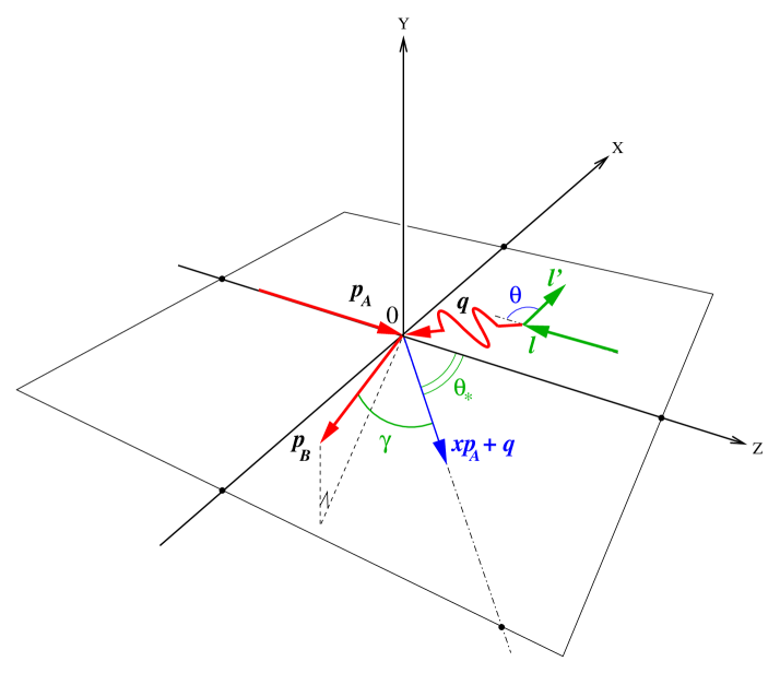
Figure 3.4: Particle momenta in the laboratory frame

3.1.4 Laboratory frame

In the laboratory frame, the electron and proton beams are collinear to the $Oz$ axis. The definition of the HERA lab frame is that the proton ($A$) moves in the $+z$ direction with energy $E_{A}$, and the incoming electron moves in the $-z$ direction with energy $E$. The momenta of the incident particles are

$$p_{A,lab}^{\mu}=\left(E_{A},0,0,E_{A}\right),$$ (3.32)

$$l_{lab}^{\mu}=\left(E,0,0,-E\right).$$ (3.33)

We can use (3.2,3.32) and (3.33) to express the Mandelstam variable $S_{eA}$ in terms of the energies $E_{A},E$ in the lab frame:

$$S_{eA}=4E_{A}E.$$ (3.34)

The outgoing electron has energy $E^{\prime}$ and scattering angle $\theta$ relative to the $-z$ direction. I define the $Ox$-axis of the HERA frame in such a way that the outgoing electron is in the $Oxz$-plane; that is,

$$l^{\prime\mu}_{lab}=\left(E^{\prime},-E^{\prime}\sin\theta,0,-E^{\prime}\cos\theta\right).$$ (3.35)

The four-momentum $q^{\mu}=l^{\mu}-l^{\prime\mu}$ of the virtual photon that probes the structure of the hadron is correspondingly

$$q_{lab}^{\mu}=\left(E-E^{\prime},E^{\prime}\sin\theta,0,-E+E^{\prime}\cos\theta\right).$$ (3.36)

The scalars $x$ and $Q^{2}$ are completely determined by measuring the energy and the scattering angle of the outgoing electron:

$$Q^{2}=2EE^{\prime}(1-\cos\theta),$$ (3.37)

$$x=\frac{EE^{\prime}(1-\cos\theta)}{E_{A}\left[2E-E^{\prime}(1+\cos\theta)\right]}.$$ (3.38)

Rather than working directly with $E^{\prime}$ and $\theta$ (or $Q^{2}$ and $x$), it is convenient to introduce another pair of variables $y$ and $\beta$:

$$y\equiv\frac{Q^{2}}{xS_{eA}}=\frac{2E-E^{\prime}(1+\cos\theta)}{2E},$$ (3.39)

and

$$\beta\equiv\frac{2xE_{A}}{Q}=\frac{\sqrt{2EE^{\prime}(1-\cos\theta)}}{2E-E^{\prime}(1+\cos\theta)}.$$ (3.40)

The variable $y$ satisfies the constraints

$$\frac{W^{2}}{S_{eA}}\leq y\leq 1,$$ (3.41)

where $W$ is defined in the previous subsection. The relationship (3.41) can be derived easily by rewriting $y$ as

$$y=1-\frac{2(p_{A}\cdot l^{\prime})}{S_{eA}}=1+\frac{T_{eA}}{S_{eA}},$$ (3.42)

where

$$T_{eA}\equiv(p_{A}-l^{\prime})^{2}.$$ (3.43)

Eq. (3.41) follows from the geometrical constraints on $T_{eA}$ for the fixed invariant mass $W^{2}$ of the final-state hadrons:

$$W^{2}-S_{eA}\leq T_{eA}\leq 0.$$ (3.44)

The observed hadron ($B$) has energy $E_{B}$ and scattering angle $\theta_{B}$ with respect to the $+z$ direction, and azimuthal angle $\varphi_{B}$; thus its momentum is

$$p_{B,lab}^{\mu}=(E_{B},E_{B}\sin\theta_{B}\cos\varphi_{B},E_{B}\sin\theta_{B}\sin\varphi_{B},E_{B}\cos\theta_{B}).$$ (3.45)

The scalars $z$ and $q_{T}^{2}$ depend on the momentum of the outgoing hadron:

$$z=\frac{\beta E_{B}(1-\cos\theta_{B})}{Q},$$ (3.46)

$$q_{T}^{2}=\frac{2E_{B}E_{0}}{z}\Biggl{[}1-\cos\gamma\Biggr{]}.$$ (3.47)

In Eq. (3.47) $\gamma$ is the angle between $\vec{p}_{B}$ and $x\vec{p}_{A}+\vec{q}$ (cf. Fig. 3.4);

$$E_{0}\equiv\frac{Q\left(1+(1-y)\beta^{2}\right)}{2\beta}$$ (3.48)

is the energy component of $xp_{A}^{\mu}+q^{\mu}$. Define $\theta_{*}$ to be the polar angle of $xp_{A}^{\mu}+q^{\mu}:$

$$xp^{\mu}_{A,lab}+q_{lab}^{\mu}\equiv E_{0}\left(1,\sin\theta_{*},0,\cos\theta_{*}\right),$$ (3.49)

where

$$cot\frac{\theta_{*}}{2}=\beta\sqrt{1-y}.$$ (3.50)

The angle $\gamma$ in Eq. (3.47) can be easily expressed in terms of the angles $\theta_{*},$ $\theta_{B}$, and $\varphi_{B}$, as

$$\cos\gamma=\cos\theta_{*}\cos\theta_{B}+\sin\theta_{*}\sin\theta_{B}\cos\varphi_{B}.$$ (3.51)

Finally, the azimuthal angle $\varphi$ of the lepton plane in the hadron frame (cf. Eqs. (3.11)) is related to the lab frame variables as

$$\cos\varphi=\frac{Q}{2q_{T}}\frac{1}{\sqrt{1-y}}\left[1-y+\frac{q_{T}^{2}}{Q^{2}}-\frac{1}{\beta^{2}}\coth^{2}\frac{\theta_{B}}{2}\right].$$ (3.52)

Figure 3.5 shows contours of constant $q_{T}$ and $\varphi$ in the plane of the angles $\theta_{B}$ and $\varphi_{B}$. The point $q_{T}=0$ corresponds to $\theta_{B}=\theta_{*},$ $\varphi_{B}=0$, in agreement with Eqs. (3.47,3.51). According to these equations, $q_{T}$ depends on $\varphi_{B}$ through $\cos\varphi_{B}$, which is a sign-even function of $\varphi_{B}$. Thus each pair of $q_{T},\,\varphi$ determines $\varphi_{B}$ up to the sign, so that the contours in Figure 3.5 are symmetric with respect to the replacement $\varphi_{B}\rightarrow-\varphi_{B}$.

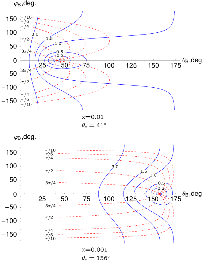
Figure 3.5: The variables $q_{T}$ and $\varphi$ as functions of the angles $\theta_{B},\,\varphi_{B}$. Solid lines are contours of constant $q_{T}$ for $q_{T}/Q$ ranging from 0.1 (the innermost contour) to 3.0. Dashed lines are contours of constant $\varphi$ for $\varphi$ ranging from $\pi/10$ to $3\pi/4$. The contour $\varphi=\pi$ coincides with the $\theta_{B}$-axis. The plots correspond to $E_{A}=820$ GeV, $E=27$ GeV, $Q=6$ GeV, $x=0.01$ (upper plot) and $x=0.001$ (lower plot).

3.1.5 Parton kinematics

The kinematical variables and momenta discussed so far are all hadron-level variables. Next, I relate these to parton variables.

Let $a$ denote the parton in $A$ that participates in the hard scattering, with momentum

$$p_{a}^{\mu}=\xi_{a}p_{A}^{\mu}.$$ (3.53)

Let $b$ denote the parton of which $B$ is a fragment, with momentum

$$p_{b}^{\mu}=p_{B}^{\mu}/\xi_{b}.$$ (3.54)

The momentum fractions $\xi_{a}$ and $\xi_{b}$ range from 0 to 1. At the parton level, I introduce the Lorentz scalars $\widehat{x},\,\,\widehat{z},\,\,\widehat{q}_{T}$ analogous to the ones at the hadron level

$$\widehat{x}=\frac{Q^{2}}{2p_{a}\cdot{q}}=\frac{x}{\xi_{a}},$$ (3.55)

$$\widehat{z}=\frac{p_{b}\cdot p_{a}}{q\cdot p_{a}}=\frac{z}{\xi_{b}},$$ (3.56)

$$\widehat{q}_{T}^{2}=-\widehat{q}_{t}^{\mu}\widehat{q}_{t\mu}.$$ (3.57)

Here $\widehat{q}_{T}^{\mu}$ is the component of $q^{\mu}$ which is orthogonal to the parton 4-momenta $p^{\mu}_{a}$ and $p^{\mu}_{b}$,

$$\widehat{q}_{t}\cdot p_{a}=\widehat{q}_{t}\cdot p_{b}=0.$$

Therefore,

$$\widehat{q}_{t}^{\mu}=q^{\mu}-p_{a}^{\mu}\frac{q\cdot p_{b}}{p_{a}\cdot p_{b}}-p_{b}^{\mu}\frac{q\cdot p_{a}}{p_{a}\cdot p_{b}}.$$ (3.58)

In the case of massless initial and final hadrons the hadronic and partonic vectors $q_{t}^{\mu}$ coincide,

$$\widehat{q}_{t}^{\mu}=q^{\mu}_{t}.$$ (3.59)

3.2 The structure of the SIDIS cross-section

The knowledge of five Lorentz scalars $S_{eA},\,\,Q,\,\,q_{T},\,\,x,\,\,z$ and the lepton azimuthal angle $\varphi$ in the hadron frame is sufficient to specify unambiguously the kinematics of the semi-inclusive scattering event $e+A\rightarrow e+B+X$. In the following, I will discuss the hadron cross-section $d\sigma_{BA}$, which is related to the parton cross-section $d\widehat{\sigma}_{ba}$ by

$$\frac{d\sigma_{BA}}{dxdzdQ^{2}dq_{T}^{2}d\varphi}=\sum_{a,b}\int_{z}^{1}\frac{d\xi_{b}}{\xi_{b}}D_{B/b}(\xi_{b},\mu_{D})\int_{x}^{1}\frac{d\xi_{a}}{\xi_{a}}F_{a/A}(\xi_{a},\mu_{F})\frac{d\widehat{\sigma}_{ba}(\mu_{F},\mu_{D})}{d\widehat{x}d\widehat{z}dQ^{2}dq_{T}^{2}d\varphi}.$$ (3.60)

Here $F_{a/A}(\xi_{a},\mu_{F})$ denotes the distribution function (PDF) of the parton of a type $a$ in the hadron $A$, and $D_{B/b}(\xi_{b},\mu_{D})$ is the fragmentation function (FF) for a parton type $b$ and the final hadron $B$. The sum over the labels $a,b$ includes contributions from all parton types, i.e., $g,u,\bar{u},d,\bar{d},\dots\,\,$. In the following, a sum over the indices $i,j$ will include contributions from active flavors of quarks and antiquarks only, i.e., it will not include a gluonic contribution. The parameters $\mu_{F}$ and $\mu_{D}$ are the factorization scales for the PDFs and FFs. To simplify the following discussion and calculations, I assume that the factorization scales $\mu_{F},\,\mu_{D}$ and the renormalization scale $\mu$ are the same:

$$\mu_{F}=\mu_{D}=\mu.$$ (3.61)

The analysis of semi-inclusive DIS can be conveniently organized by separating the dependence of the parton and hadron cross-sections on the leptonic angle $\varphi$ and the boost parameter $\psi$ from the other kinematical variables $x,\,\,z,\,\,Q$ and $q_{T}$ [83]. This separation does not depend on the details of the hadronic dynamics. Following [34], I express the hadron (or parton) cross-section as a sum over products of functions of these lepton angles in the hadron frame $A_{\rho}(\psi,\varphi)$, and structure functions $\,{}^{\rho}V_{BA}(x,z,Q^{2},q_{T}^{2})$ (or ${\,}^{\rho}\widehat{V}_{ba}(\widehat{x},\widehat{z},Q^{2},q_{T}^{2},\mu)$, respectively):

$$\frac{d\sigma_{BA}}{dxdzdQ^{2}dq_{T}^{2}d\varphi}=\sum_{\rho=1}^{4}{\,}^{\rho}V_{BA}(x,z,Q^{2},q_{T}^{2})A_{\rho}(\psi,\varphi),$$ (3.62)

$$\frac{d\widehat{\sigma}_{ba}(\mu)}{d\widehat{x}d\widehat{z}dQ^{2}dq_{T}^{2}d\varphi}=\sum_{\rho=1}^{4}{\,}^{\rho}\widehat{V}_{ba}(\widehat{x},\widehat{z},Q^{2},q_{T}^{2},\mu)A_{\rho}(\psi,\varphi).$$ (3.63)

The coefficients ${\,}^{\rho}V_{BA}$ (or ${\,}^{\rho}\widehat{V}_{ba}$) of the angular functions $A_{\rho}(\psi,\varphi)$ are independent of one another.

At the energy of HERA, hadroproduction via parity-violating $Z$-boson exchanges can be neglected, and only four out of the nine angular functions listed in [34] contribute to the cross-sections (3.62-3.63). They are

$$A_{1}=1+\cosh^{2}\psi, A_{3}=-\cos\varphi\sinh 2\psi,$$

$$A_{2}=-2, A_{4}=\cos 2\varphi\sinh^{2}\psi.$$ (3.64)

Figure 3.6: Feynman diagrams for semi-inclusive DIS: (a) LO; (b-d) NLO virtual diagrams; (e-f) NLO real emission diagrams

Out of the four structure functions, ${\,}^{1}\widehat{V}_{ba}$ for the angular function $A_{1}=1+\cosh^{2}\psi$ has a special status, since only ${\,}^{1}\widehat{V}_{ba}$ receives contributions from the lowest order of PQCD (Figure 3.6a). At ${\cal O}(\alpha_{S})$, only the contribution to the ${\,}^{1}\widehat{V}_{ba}$ structure function diverges in the limit $q_{T}\rightarrow 0$.

3.3 Leading-order cross section

Consider first the ${\cal O}(\alpha_{S}^{0})$ process of the quark-photon scattering (Fig. 3.6a). This process contributes to the total rate of SIDIS at the leading order (LO). There is no LO contribution from gluons. Due to the conservation of the 4-momentum in the parton-level diagram, at this order

$$p^{\nu}_{b}=p^{\nu}_{a}+q^{\nu}.$$ (3.65)

This condition and Eqs. (3.58,3.59) imply that

$$q_{T}^{2}=-q_{t}\cdot q_{t}=0.$$ (3.66)

Also the longitudinal variables are

$$\xi_{a}=x, \xi_{b}=z,$$

$$\widehat{x}= \widehat{z} =1,$$ (3.67)

so that the momentum of the final-state hadron $B$ is

$$p_{B}^{\mu}=z\,\left(xp_{A}^{\mu}+q^{\mu}\right).$$ (3.68)

Since both quarks and electrons are spin-1/2 particles, the LO cross section is proportional to $1+\cosh^{2}\psi\equiv A_{1}(\psi,\varphi)$ (Callan-Gross relation [84]). Hence the LO cross section is

$$\left.\frac{d\widehat{\sigma}_{ij}}{dxdzdQ^{2}dq_{T}^{2}d\varphi}\right|_{LO}=\frac{\sigma_{0}F_{l}}{S_{eA}}\delta(\vec{q}_{T})\frac{A_{1}(\psi,\varphi)}{2}\delta_{ij}e_{j}^{2}\delta(1-\widehat{x})\delta(1-\widehat{z}),$$ (3.69)

where $\vec{q}_{T}\equiv(0,q_{T},0,0)$ in the hadron frame. In Eq. (3.69) the parameter $\sigma_{0}$ collects various constant factors coming from the hadronic side of the matrix element,

$$\sigma_{0}\equiv\frac{Q^{2}}{4\pi S_{eA}x^{2}}\Bigl{(}\frac{e^{2}}{2}\Bigr{)}.$$ (3.70)

The factor $F_{l}$ that comes from the leptonic side is defined by

$$F_{l}=\frac{e^{2}}{2}\frac{1}{Q^{2}}.$$ (3.71)

$e_{j}$ denotes the fractional electric charge of a participating quark or antiquark of the flavor $j$; $e_{j}=2/3$ for up quarks and $-1/3$ for down quarks.

The LO cross section (3.69) does not explicitly depend on $Q^{2}$, but rather on $x$ and $z$. This phenomenon is completely analogous to the Bjorken scaling in completely inclusive DIS [4], i.e., independence of DIS structure functions from the photon’s virtuality $Q^{2}$. Just as in the case of inclusive DIS, the scaling of the LO SIDIS cross section is approximate due to the dependence of PDFs and FFs on the factorization scale $\mu$. This scale is naturally chosen of order $Q$, the only momentum scale in the LO kinematics. When $\mu\approx Q$ varies, the PDFs and FFs change according to Dokshitser-Gribov-Lipatov-Altarelli-Parisi (DGLAP) differential equations (2.29,2.31). By solving the DGLAP equations, one sums dominant contributions from the collinear radiation along the directions of the hadrons $A$ and $B$ through all orders of PQCD. Formally, the scale dependence of the PDFs and FFs is an ${\cal O}(\alpha_{S})$ effect, so that it is on the same footing in the LO calculation as other neglected higher-order QCD corrections. By observing the dependence of the LO cross section on $\mu$, we can qualitatively test the importance of such neglected corrections. One finds that this dependence is substantial, so that a calculation of ${\cal O}(\alpha_{S})$ corrections is needed to reduce theoretical uncertainties. Let us now turn to this more elaborate calculation.

3.4 The higher-order radiative corrections

The complete set of ${\cal O}(\alpha_{S})$ corrections to the SIDIS cross section is shown in Figs. 3.6b-f. These corrections contribute to the total rate at the next-to-leading order (NLO).

At this order, one has to account for the virtual corrections to the LO subprocess $\stackrel{{\scriptstyle(-)}}{{q}}\gamma^{*}\rightarrow\stackrel{{\scriptstyle(-)}}{{q}}$ (Figs. 3.6b-d), as well as for the diagrams describing the real emission subprocesses $\stackrel{{\scriptstyle(-)}}{{q}}\gamma^{*}\rightarrow\stackrel{{\scriptstyle(-)}}{{q}}g$ and $g\gamma^{*}\rightarrow q\bar{q}$, with the subsequent fragmentation of the final-state quark, antiquark or gluon (Figs. 3.6e-f). The explicit expression for the ${\cal O}(\alpha_{S})$ cross section is given in Appendix A.

Due to the momentum conservation, the momentum of the unobserved final-state partons (e.g. the gluon in Fig. 3.6e) can be expressed in terms of $q^{\mu},\,p^{\mu}_{a},\,p_{b}^{\mu}$:

$$p_{x}^{\mu}=q^{\mu}+p_{a}^{\mu}-p_{b}^{\mu}.$$ (3.72)

When there is no QCD radiation ($p_{x}^{\mu}=0$), the momentum of $b$ satisfies the leading-order relationship $p_{b}^{\mu}=p_{a}^{\mu}+q^{\mu}$, so that $q_{T}=0$. If $q_{T}/Q\ll 1$, the perturbative parton-level cross section is dominated by the term with $\rho=1$. In the limit $q_{T}^{2}/Q^{2}\rightarrow 0$, but $q_{T}\neq 0$, ${\,}^{1}{\widehat{V}_{ba}}$ behaves as $1/q_{T}^{2}$ times a series in powers of $\alpha_{S}$ and logarithms $\ln(q_{T}^{2}/Q^{2}$),

$${\,}^{1}{\widehat{V}}_{ba}\approx\frac{\sigma_{0}F_{l}}{2\pi S_{eA}}\frac{1}{q_{T}^{2}}\sum_{k=1}^{\infty}\Biggl{(}\frac{\alpha_{S}}{\pi}\Biggr{)}^{k}\sum_{m=0}^{2k-1}\widehat{v}^{(km)}_{ba}(\widehat{x},\widehat{z})\ln^{m}\Biggl{(}\frac{q_{T}^{2}}{Q^{2}}\Biggr{)},$$ (3.73)

where the coefficients $\widehat{v}^{(km)}_{ba}(\widehat{x},\widehat{z})$ are generalized functions of the variables $\widehat{x}$ and $\widehat{z}$. Obviously, the coefficient of the order $\alpha_{S}^{k}$ in Eq. (3.73) coincides with the most divergent part of the ${\cal O}(\alpha_{S}^{k})$ correction to the SIDIS cross section from the real emission subprocesses. This coefficient will be called the asymptotic part of the real emission correction to ${\,}^{1}{\widehat{V}}_{ba}$ at ${\cal O}(\alpha_{S}^{k})$.

Convergence of the series in (3.73) deteriorates rapidly as $q_{T}/Q\rightarrow 0$ because of the growth of the terms $(q_{T}^{-2})\ln^{m}(q_{T}^{2}/Q^{2})$. Ultimately the structure function ${\,}^{1}{\widehat{V}_{ba}}$ has a non-integrable singularity at $q_{T}=0$. Its asymptotic behavior is very different from that of the structure functions ${\,}^{2,3,4}{\widehat{V}_{ba}}$, which are less singular and, in fact, integrable at $q_{T}=0$. This singular behavior of ${\,}^{1}{\widehat{V}_{ba}}$ is generated by infrared singularities of the perturbative cross section that are located at $q_{T}=0$. Indeed, according to the discussion in Section 2.3, the diagrams with the emission of massless particles generate singularities when the momentum $p_{1}^{\beta}$ of one of the particles is soft ($p_{1}^{\beta}\rightarrow 0$) or collinear to the momentum $p_{2}^{\beta}$ of another participating particle ($p_{1\beta}p_{2}^{\beta}=0$). The soft singularities in the real emission corrections cancel with the soft singularities in the virtual corrections. For instance, at ${\cal O}(\alpha_{S})$ the soft singularities of the diagrams shown in Fig. 3.6e-f cancel with the soft singularities of the diagrams shown in Fig. 3.6b-d. The remaining collinear singularities are included in the PDFs and FFs, so that they should be subtracted from ${\,}^{1}{\widehat{V}_{ba}}$.

There exist two qualitatively different approaches for handling such singularities. The first approach deals with the singularities order by order in perturbation theory; the second approach identifies and sums the most singular terms in all orders of the perturbative expansion. In the next two Subsections, I discuss regularization of infrared singularities in each of these two approaches.

3.4.1 Factorization of collinear singularities at ${\cal O}(\alpha_{S})$

Let us begin by considering the first approach, in which singularities are regularized independently at each order of the series in $\alpha_{S}$. The singularity in the ${\mathcal{O}}(\alpha_{S})$ part of the asymptotic expansion (3.73) can be regularized by introducing a “separation scale” $q_{T}^{S}$ and considering the fixed-order cross section separately in the regions $0\leq q_{T}\leq q_{T}^{S}$ and $q_{T}>q_{T}^{S}$. The value of $q_{T}^{S}$ should be small enough for the approximation (3.73) to be valid over the whole range $q_{T}\leq q_{T}^{S}$.

The quantity $q_{T}^{S}$ plays the role of a phase space slicing parameter. In the region $0\leq q_{T}\leq q_{T}^{S}$, we can apply the modified minimal subtraction ($\overline{MS}$) factorization scheme [43] to take care of the singularities at $q_{T}=0$. In the $\overline{MS}$ scheme, the regularization is done through continuation of the parton-level cross section to $n=4-2\epsilon,\,\,\epsilon>0$ dimensions [42]. The $n$-dimensional expression for the ${\cal O}(\alpha_{S})$ part of the asymptotic expansion (3.73) of ${\,}^{1}{\widehat{V}}_{ba}(\widehat{x},\widehat{z},Q^{2},q_{T}^{2})$ is

$$\left.{\,}^{1}{\widehat{V}}_{ba}\right|_{\displaystyle 1/q_{T}^{2},{\cal O}(\alpha_{S})}=\left(\frac{2\pi\mu_{n}}{\widehat{z}}\right)^{4-n}\frac{\sigma_{0}F_{l}}{2\pi S_{eA}}\frac{\alpha_{S}}{\pi}\frac{1}{2q_{T}^{2}}\sum_{j}\delta_{bj}\delta_{ja}e_{j}^{2}\times$$ (3.74)

$$\Biggl{[}\delta(1-\widehat{z})\left\{P^{(1)}_{qq}(\widehat{x})+P^{(1)}_{qg}(\widehat{x})\right\}+\left\{P^{(1)}_{qq}(\widehat{z})+P^{(1)}_{gq}(\widehat{z})\right\}\delta(1-\widehat{x})$$

$$+ 2\delta(1-\widehat{z})\delta(1-\widehat{x})\left[C_{F}\log\frac{Q^{2}}{q_{T}^{2}}-\frac{3}{2}C_{F}\right]+{\mathcal{O}}\Bigl{(}\frac{\alpha_{S}}{\pi},q_{T}^{2}\Bigr{)}\Biggr{]}.$$

Here the color factor $C_{F}=(N_{c}^{2}-1)/(2N_{c})=4/3,$ $N_{c}=3$ is the number of quark colors in QCD. The functions $P^{(1)}_{ij}(\xi)$ entering the convolution integrals in (3.74) are the unpolarized ${\cal O}(\alpha_{S})$ splitting kernels [47]:

$$P^{(1)}_{qq}(\xi) = C_{F}\left[\frac{1+\xi^{2}}{1-\xi}\right]_{+},$$ (3.75)

$$P^{(1)}_{qg}(\xi) = \frac{1}{2}\left(1-2\xi+2\xi^{2}\right),$$ (3.76)

$$P^{(1)}_{gq}(\xi) = C_{F}\frac{1+(1-\xi)^{2}}{\xi}.$$ (3.77)

The “+”-prescription in $P^{(1)}_{qq}(\xi)$ regularizes $P^{(1)}_{qq}(\xi)$ at $\xi=1$; it is defined as

$$\int_{0}^{1}d\xi\,\left[f(\xi)\right]_{+}g(\xi)\equiv\int_{0}^{1}d\xi\,f(\xi)\,\left(g(\xi)-g(1)\right).$$

The scale parameter $\mu_{n}$ in (3.74) is introduced to restore the correct dimensionality of the parton-level cross section $d\widehat{\sigma}_{ba}/(d\widehat{x}d\widehat{z}dQ^{2}dq_{T}^{n-2}d\varphi)$ for $n\neq 4$. The soft and collinear singularities appear as terms proportional to $1/\epsilon^{2}$ and $1/\epsilon$ when $n\rightarrow 4$. The soft singularity in the real emission corrections cancels with the soft singularity in the virtual corrections. At ${\cal O}(\alpha_{S}),$ the virtual corrections (Fig.  3.6b-d) evaluate to

$$\left.\frac{d\widehat{\sigma}_{ba}}{dxdzdQ^{2}dq_{T}^{2}d\varphi}\right|_{\displaystyle virt,{\cal O}(\alpha_{S})} = -\frac{\alpha_{S}}{2\pi}C_{F}\left(\frac{4\pi\mu_{n}^{2}}{Q^{2}}\right)^{\epsilon}\frac{1}{\Gamma(1-\epsilon)}\left(\frac{2}{\epsilon^{2}}+\frac{3}{\epsilon}+8\right)\times$$ (3.78)

$$\times \left.\frac{d\widehat{\sigma}_{ba}}{dxdzdQ^{2}dq_{T}^{2}d\varphi}\right|_{LO},$$

where the LO cross section is given in Eq. (3.69).

The remaining collinear singularities are absorbed into the partonic PDFs and FFs. When the partonic PDFs and FFs are subtracted from the partonic cross section $d\widehat{\sigma}$, the remainder is finite and independent of the types of the external hadrons. We denote this finite remainder as $(d\widehat{\sigma})_{hard}$. The convolution of $(d\widehat{\sigma})_{hard}$ with the hadronic PDFs and FFs yields a cross section for the external hadronic states $A$ and $B$. The “hard” part depends on an arbitrary factorization scale $\mu$ through terms like $P^{(1)}_{ab}\ln(\mu/K)$, where $P^{(1)}_{ab}(\xi)$ are splitting functions, and $K$ is some momentum scale in the process. The scales $\mu$ and $\mu_{n}$ are related as

$$\mu^{2}=4\pi e^{-\gamma_{E}}\mu_{n}^{2}.$$

The dependence on the factorization scale in the hard part is compensated, up to higher-order terms in $\alpha_{S}$, by scale dependence of the long-distance hadronic functions.

After the cancellation of soft singularities and factorization of collinear singularities, one can calculate analytically the integral of $({\,}^{1}{\widehat{V}_{ba}})_{hard}$ over the region $0\nolinebreak\leq\nolinebreak q_{T}\nolinebreak\leq\nolinebreak q_{T}^{S}$. At ${\mathcal{O}}(\alpha_{S})$ this integral is given by

$$\int_{0}^{(q_{T}^{S})^{2}}dq_{T}^{2}\left({\,}^{1}{\widehat{V}_{ba}}\right)_{hard}=\frac{\sigma_{0}F_{l}}{2\pi S_{eA}}\sum_{j}e_{j}^{2}\Biggl{\{}{\,}^{1}{\widehat{V}^{LO}_{ba,j}}+\frac{\alpha_{S}}{\pi}{\,}^{1}{\widehat{V}^{NLO}_{ba,j}}\Biggr{\}}.$$ (3.79)

The LO and NLO structure functions are

$${\,}^{1}{\widehat{V}^{LO}_{ba,j}} = \delta(1-\widehat{z})\delta(1-\widehat{x})\delta_{bj}\delta_{ja},$$ (3.80)

$${\,}^{1}{\widehat{V}^{NLO}_{ba,j}} = -\frac{1}{2}\Biggl{[}\Biggl{(}C_{F}\ln^{2}{\frac{Q^{2}}{(q_{T}^{S})^{2}}}-3C_{F}\ln{\frac{Q^{2}}{(q_{T}^{S})^{2}}}\Biggr{)}\delta(1-\widehat{z})\delta(1-\widehat{x})\delta_{bj}\delta_{ja}$$ (3.81)

$$+ \ln{\frac{\mu^{2}}{(\widehat{z}\,q_{T}^{S})^{2}}}\biggl{(}\delta(1-\widehat{z})\delta_{bj}P^{(1)}_{ja}(\widehat{x})+P^{(1)}_{bj}(\widehat{z})\delta(1-\widehat{x})\delta_{ja}\biggr{)}\Biggr{]}$$

$$+ \delta(1-\widehat{z})\delta_{bj}{c}^{in(1)}_{ja}(\widehat{x})+{c}^{out(1)}_{bj}(\widehat{z})\delta(1-\widehat{x})\delta_{ja}.$$

The coefficient functions ${c}^{in,out(1)}_{ba}(\xi)$ that appear in ${\,}^{1}{\widehat{V}^{NLO}_{ba,j}}$ are given by

$${c}^{(1)in}_{ji}(\xi)={c}^{out(1)}_{ij}(\xi) = \delta_{ij}C_{F}\Biggl{[}\frac{1}{2}(1-\xi)-2\delta(1-\xi)\Biggr{]},$$ (3.82)

$${c}^{(1)in}_{jg}(\xi) = \frac{1}{2}\xi(1-\xi),$$ (3.83)

$${c}^{(1)out}_{gj}(\xi) = \frac{C_{F}}{2}\xi.$$ (3.84)

Now consider the kinematical region $q_{T}>q_{T}^{S}$, where the approximation (3.74) no longer holds. In this region, $({\,}^{1}{\widehat{V}_{ba}})_{hard}$ should be obtained from the exact NLO result. With this prescription, the integral over $q_{T}^{2}$ can be calculated as

$$\int_{0}^{\max q_{T}^{2}}dq_{T}^{2}\frac{d\widehat{\sigma}_{ba}}{d\widehat{x}d\widehat{z}dQ^{2}dq_{T}^{2}d\varphi} =$$

$$A_{1}(\psi,\varphi)\Biggl{\{}\int_{0}^{(q_{T}^{S})^{2}}dq_{T}^{2}\left({\,}^{1}{\widehat{V}_{ba}}\right)_{hard} + \int_{(q_{T}^{S})^{2}}^{\max q_{T}^{2}}dq_{T}^{2}\left({\,}^{1}{\widehat{V}_{ba}}\right)_{hard}\Biggr{\}}$$

$$+\sum_{\rho=2}^{4}A_{\rho}(\psi,\varphi)\int_{0}^{\max q_{T}^{2}}dq_{T}^{2}\left({\,}^{\rho}{\widehat{V}_{ba}}\right),$$ (3.85)

where $\max q_{T}^{2}$ is the maximal value of $q_{T}^{2}$ allowed by kinematics. The first integral on the right-hand side is calculated analytically, using the approximation (3.79); the second and third integrals are calculated numerically, using the complete perturbative result of the order ${\mathcal{O}}(\alpha_{S})$. The numerical calculation is done with the help of a Monte Carlo integration package written in the style of the programs Legacy and ResBos used earlier for resummation in vector boson production at hadron-hadron colliders [25].

3.4.2 All-order resummation of large logarithmic terms

A significant failure of the computational procedure in (3.85) is that it cannot be applied to the description of the $q_{T}$-dependent differential cross sections. Indeed, the cancellation of the infrared singularities is achieved by integration of the cross section over the region $0\leq q_{T}\leq q_{T}^{S}$. However the shape of the $q_{T}$ distribution is arbitrary and depends on the choice of the parameter $q_{T}^{S}$ that specifies the lowest $q_{T}$ bin $0\leq q_{T}\leq q_{T}^{S}$. The fundamental problem is that the terms in (3.73) with small powers of $\alpha_{S}$ do not reliably approximate the complete sum in the region $q_{T}\ll Q$.

This problem justifies the second approach to the regularization of the singularities at $q_{T}=0$, in which large logarithms in (3.73) and virtual corrections at $q_{T}=0$ are summed to all orders. A better approximation for ${\,}^{1}{\widehat{V}}_{ba}$ at $q_{T}/Q\ll 1$ is provided by the Fourier transform of a $\vec{b}$-space function $\widehat{\widetilde{W}}_{ba}(b,Q,\widehat{x},\widehat{z},\mu)$, which sums the dominant terms in (3.73) and virtual corrections through all orders of $\alpha_{S}$:

$$\left.{\,}^{1}{\widehat{V}}_{ba}(\widehat{x},\widehat{z},Q^{2},q_{T}^{2},\mu)\right|_{\widetilde{W}}=\frac{\sigma_{0}F_{l}}{2S_{eA}}\int\frac{d^{2}b}{(2\pi)^{2}}e^{i\vec{q}_{T}\cdot\vec{b}}\widehat{\widetilde{W}}_{ba}(b,Q,\widehat{x},\widehat{z},\mu).$$ (3.86)

Here $\vec{b}$ is a vector conjugate to $\vec{q}_{T}$, and $b$ denotes the magnitude of $\vec{b}$. Hence ${\,}^{1}\widehat{V}_{ba}$ at all values of $q_{T}$ can be approximated by

$${\,}^{1}\widehat{V}_{ba}(\widehat{x},\widehat{z},Q^{2},q_{T}^{2},\mu)=\left.{\,}^{1}{\widehat{V}}_{ba}(\widehat{x},\widehat{z},Q^{2},q_{T}^{2},\mu)\right|_{\widetilde{W}}+{\,}^{1}\widehat{Y}_{ba}(\widehat{x},\widehat{z},Q^{2},q_{T}^{2}),$$ (3.87)

where ${\,}^{1}\widehat{Y}_{ba}$ is the difference between the ${\cal O}(\alpha_{S})$ expression for ${\,}^{1}\widehat{V}_{ba}$ (cf. Appendix A) and ${\cal O}(\alpha_{S})$ asymptotic part (3.74), taken at $n=4$. This difference is finite in the limit $q_{T}\rightarrow 0$.

The complete hadron-level resummed cross section can be obtained by including the finite parton structure functions for $\rho=2,3,4$ and convolving the parton-level structure functions with PDFs and FFs (cf. Eqs. (3.60-3.63)):

$$\left.\frac{d\sigma_{BA}}{dxdzdQ^{2}dq_{T}^{2}d\varphi}\right|_{resum}=\frac{\sigma_{0}F_{l}}{S_{eA}}\frac{A_{1}(\psi,\varphi)}{2}\int\frac{d^{2}b}{(2\pi)^{2}}e^{i\vec{q}_{T}\cdot\vec{b}}\widetilde{W}_{BA}(b,Q,x,z)+Y_{BA}.$$ (3.88)

In this equation, the hadron-level $b$-dependent form-factor $\widetilde{W}_{BA}(b,Q,x,z)$ is the sum of convolutions of parton-level form-factors $\widehat{\widetilde{W}}_{ba}(b,Q,\widehat{x},\widehat{z})$ with the PDFs and FFs:

$$\widetilde{W}_{BA}=\sum_{a,b}D_{B/b}\otimes\widehat{\widetilde{W}}_{ba}\otimes F_{a/A}.$$ (3.89)

$Y_{BA}$ denotes the complete finite piece,

$$Y_{BA}\equiv{\,}^{1}Y_{BA}+\sum_{\rho=2}^{4}{\,}^{\rho}V_{BA}A_{\rho}(\psi,\varphi),$$ (3.90)

where

$${\,}^{1}{Y}_{BA}\equiv\sum_{a,b}D_{B/b}\otimes{\,}^{1}{\widehat{Y}}_{ba}\otimes F_{a/A}.$$ (3.91)

The explicit expression for $Y_{BA}$ is presented in Appendix A.
At small $b$ and large $Q$ (i.e., in the region where perturbative dynamics is expected to dominate) the general structure of $\widetilde{W}_{BA}(b,Q,x,z)$ can be found from first principles [17, 21]:

$$\widetilde{W}_{BA}(b,Q,x,z)=\sum_{j}e_{j}^{2}(D_{B/b}\otimes{\cal C}^{out}_{bj})(z,b)({\cal C}_{ja}^{in}\otimes F_{a/A})(x,b)e^{-S_{BA}(b,Q)}.$$ (3.92)

According to the discussion in Section 2.4, the form-factor $\widetilde{W}_{BA}$ is the all-order sum of the large logarithms, which remain after the cancellation of soft singularities and factorization of collinear singularities. The soft contributions are included in the Sudakov function $S_{BA}(b,Q)$. At small $b$, $S_{BA}(b,Q)$ does not depend on the types of the external hadrons and looks like

$$S_{BA}(b,Q)=\int_{C_{1}^{2}/b^{2}}^{C_{2}^{2}Q^{2}}\frac{d\overline{\mu}^{2}}{\overline{\mu}^{2}}\left({\cal A}(\alpha_{S}(\overline{\mu}),C_{1})\ln\frac{C_{2}^{2}Q^{2}}{\overline{\mu}^{2}}+{\cal B}(\alpha_{S}(\overline{\mu}),C_{1},C_{2})\right)\equiv S^{P}(b,Q),$$ (3.93)

with

$${\cal A}(\alpha_{S}(\overline{\mu}),C_{1}) = \sum_{k=1}^{\infty}{\cal A}_{k}(C_{1})\Biggl{(}\frac{\alpha_{S}(\overline{\mu})}{\pi}\Biggr{)}^{k},$$ (3.94)

$${\cal B}(\alpha_{S}(\overline{\mu}),C_{1},C_{2}) = \sum_{k=1}^{\infty}{\cal B}_{k}(C_{1},C_{2})\Biggl{(}\frac{\alpha_{S}(\overline{\mu})}{\pi}\Biggr{)}^{k}.$$ (3.95)

Contributions from the collinear partons are included in the functions ${\cal\mathcal{C}}^{in}(\widehat{x},b,\mu)$ and ${\cal\mathcal{C}}^{out}(\widehat{z},b,\mu)$. These functions can also be expanded in series of $\alpha_{S}/\pi$, as

$${\cal\mathcal{C}}^{in}_{ij}(\widehat{x},b,\mu)=\sum_{k=0}^{\infty}{\cal\mathcal{C}}^{in(k)}_{ij}(\widehat{x},C_{1},C_{2,}\mu b)\Biggl{(}\frac{\alpha_{S}(\mu)}{\pi}\Biggr{)}^{k},$$ (3.96)

$${\cal\mathcal{C}}^{out}_{ij}(\widehat{z},b,\mu)=\sum_{k=0}^{\infty}{\cal\mathcal{C}}^{out(k)}_{ij}(\widehat{z},C_{1},C_{2},\mu b)\Biggl{(}\frac{\alpha_{S}(\mu)}{\pi}\Biggr{)}^{k}.$$ (3.97)

According to Eq. (3.93), the integration in $S^{P}(b,Q)$ is performed between two scales $C_{1}/b$ and $C_{2}Q$, where $C_{1}$ and $C_{2}$ are constants of order 1. These constants also appear in terms proportional to $\delta(1-\widehat{x})$ or $\delta(1-\widehat{z})$ in the ${\cal C}$-functions. The complete factor $\widetilde{W}(b,Q)$ is approximately independent from $C_{1}$ and $C_{2}$. In addition, the ${\cal\mathcal{C}}$-functions depend on the factorization scale $\mu$ that separates singular collinear contributions included in the PDFs and FFs from the finite collinear contributions included in the ${\cal C}$-functions. To suppress certain logarithms in ${\cal O}(\alpha_{S})$ parts of the ${\cal C}^{in}$ and ${\cal C}^{out}$ functions, it is convenient to choose

$$C_{1} = 2e^{-\gamma_{E}}\equiv b_{0},$$ (3.98)

$$C_{2} = 1,$$ (3.99)

$$\mu = b_{0}/b,$$ (3.100)

where $\gamma_{E}=0.577215...$ is the Euler constant.

Using our NLO results, I find the following expressions for the coefficients ${\cal A}_{k}(C_{1})$, ${\cal B}_{k}(C_{1},C_{2})$ and the ${\cal C}$-functions:

$${\cal A}_{1} = C_{F},$$ (3.101)

$${\cal B}_{1} = 2C_{F}\log\biggl{(}\frac{e^{-3/4}C_{1}}{b_{0}C_{2}}\biggr{)}.$$ (3.102)

To the same order, the expressions for the $\mathcal{C}$-functions are

• LO:

  $${\cal\mathcal{C}}^{in(0)}_{jk}(\widehat{x},\mu b) = \delta_{jk}\delta(1-\widehat{x}),$$ (3.103)

  $${\cal\mathcal{C}}^{out(0)}_{jk}(\widehat{z},\mu b) = \delta_{jk}\delta(1-\widehat{z}),$$ (3.104)

  $${\cal\mathcal{C}}^{in(0)}_{jg}= {\cal\mathcal{C}}^{out(0)}_{gj} =0;$$ (3.105)

• NLO:

  $${\cal\mathcal{C}}^{in(1)}_{jk}(\widehat{x},\mu b) = \frac{C_{F}}{2}(1-\widehat{x})-P^{(1)}_{qq}(\widehat{x})\log\Bigl{(}\frac{\mu b}{b_{0}}\Bigr{)}$$ (3.106)

  $$- C_{F}\delta(1-\widehat{x})\biggl{(}\frac{23}{16}+\log^{2}\Bigl{(}\frac{e^{-3/4}C_{1}}{b_{0}C_{2}}\Bigr{)}\biggr{)},$$

  $${\cal\mathcal{C}}^{in(1)}_{jg}(\widehat{x},\mu b) = \frac{1}{2}\widehat{x}(1-\widehat{x})-P^{(1)}_{qg}(\widehat{x})\log\Bigl{(}\frac{\mu b}{b_{0}}\Bigr{)},$$ (3.107)

  $${\cal\mathcal{C}}^{out(1)}_{jk}(\widehat{z},\mu b) = \frac{C_{F}}{2}(1-\widehat{z})-P^{(1)}_{qq}(\widehat{z})\log\Bigl{(}\frac{\mu b}{\widehat{z}b_{0}}\Bigr{)}$$ (3.108)

  $$- C_{F}\delta(1-\widehat{z})\biggl{(}\frac{23}{16}+\log^{2}\Bigl{(}\frac{e^{-3/4}C_{1}}{b_{0}C_{2}}\Bigr{)}\biggr{)},$$

  $${\cal\mathcal{C}}^{out(1)}_{gj}(\widehat{z},\mu b) = \frac{C_{F}}{2}\widehat{z}-P^{(1)}_{gq}(\widehat{z})\log\Bigl{(}\frac{\mu b}{\widehat{z}b_{0}}\Bigr{)}.$$ (3.109)

In these formulas, the indices $j$ and $k$ correspond to quarks and antiquarks, and $g$ to gluons. In Appendix B I show that the expansion of the integral over $b$ in Eq. (3.88) up to the order ${\cal O}(\alpha_{S})$, with perturbative coefficients given in Eqs. (3.101-3.109), reproduces the small-$q_{T}$ limit of the fixed-order ${\cal O}(\alpha_{S})$ cross section discussed in Subsection 3.4.1.

Due to the crossing relations between parton-level SIDIS, vector boson production, and $e^{+}e^{-}$ hadroproduction, the ${\cal\mathcal{C}}^{in}$-functions are essentially the same in SIDIS and the Drell-Yan process; and the ${\cal\mathcal{C}}^{out}$-functions are essentially the same in SIDIS and $e^{+}e^{-}$ hadroproduction. At NLO the only difference stems from the fact that the momentum transfer $q^{2}$ is spacelike in DIS and timelike in the other two processes. Hence the virtual diagrams Figs. 3.6b-d differ by $\pi^{2}$ for spacelike and timelike $q^{2}$. Correspondingly, ${\cal\mathcal{C}}^{in(1)}_{jk}$ for SIDIS does not contain the term $(\pi^{2}/3)\delta(1-\widehat{x})$, which is present in the ${\cal\mathcal{C}}^{in(1)}_{jk}$-function for the Drell-Yan process. Similarly, ${\cal\mathcal{C}}^{out(1)}_{jk}$ for SIDIS does not contain the term $(\pi^{2}/3)\delta(1-\widehat{z})$, which is present in the ${\cal\mathcal{C}}^{out(1)}_{jk}$-function for $e^{+}e^{-}$ hadroproduction.

Up to now, I was discussing the behavior of the resummed cross-section at short distances. The representation (3.92) should be modified at large values of the variable $b$ to account for nonperturbative long-distance dynamics. The authors of Ref. [21] suggested the following ansatz for $\widetilde{W}_{BA}$ which is valid at all values of $b$:

$$\widetilde{W}_{BA}(b,Q,x,z)=\sum_{j}e_{j}^{2}(D_{B/b}\otimes{\cal\mathcal{C}}^{out}_{bj})(z,b_{*})({\cal\mathcal{C}}_{ja}^{in}\otimes F_{a/A})(x,b_{*})e^{-S_{BA}}.$$ (3.110)

Here the variable

$$b_{*}\equiv\frac{b}{\sqrt{1+\Bigl{(}\frac{b}{b_{max}}\Bigr{)}^{2}}}$$ (3.111)

serves to reproduce the perturbative solution (3.92) at $b\ll b_{max}$, with $b_{max}\approx 0.5\mbox{\, GeV}^{-1}$, and turn off the perturbative dynamics for $b\geq b_{max}$. Furthermore, the Sudakov factor is modified, being written as the sum of the perturbatively calculable part $S^{P}(b_{*},Q)$ given by Eq. (3.93), and a nonperturbative part, which is only partially constrained by the theory:

$$S_{BA}(b,Q,x,z)=S^{P}(b_{*},Q,x,z)+S^{NP}_{BA}(b,Q,x,z).$$ (3.112)

An explicit solution for the function $S_{BA}^{NP}(b,Q,x,z)$ has not been found yet. Nonetheless, the renormalization properties of the theory require that the $Q$ dependence in the nonperturbative Sudakov term be separated from the dependence on the other kinematical variables, i.e.,

$$S^{NP}_{BA}(b,Q,x,z)=g_{BA}^{(1)}(b,x,z)+g_{BA}^{(2)}(b,x,z)\log\frac{Q}{Q_{0}},$$ (3.113)

with $Q_{0}\approx 1\,\,\mbox{\, GeV}$. The theory does not predict the functional forms of $g_{BA}^{(1)}(b,x,z)$ and $g_{BA}^{(2)}(b,x,z)$, so these must be determined by fitting experimental data. In addition, if $S^{NP}_{BA}(b,Q,x,z)$ indeed describes long-distance dynamics, it should vanish or be much smaller than $S^{P}(b,Q,x,z)$ in the perturbative region $b<b_{max}.$ In the analysis of the experimental results, we may find that the fit to the data prefers a parametrization of $S^{NP}(b)$ that is not small in comparison to the perturbative part of $\widetilde{W}_{BA}$ at $b<b_{max}$. Such observation will be an evidence in favor of important dynamics that is not included in the $b$-space resummation formula with coefficients calculated at the given order of PQCD. Therefore, this work uses an interpretation of $S^{NP}$ that is broader than its original definition in [21]. $S^{NP}$ will parametrize not only large-$b$ physics, but additional contributions to $\widetilde{W}_{BA}$ at all values of $b$ that are not included in the perturbative part of $\widetilde{W}_{BA}$. In the following parts of the thesis I will test whether the data are consistent with the assumption that these additional contributions are small in comparison to the perturbative part of $\widetilde{W}_{BA}$ when $b<b_{max}$.

Before ending this section, I would like to comment on a subtle difference between ${\cal\mathcal{C}}^{in}$ and ${\cal\mathcal{C}}^{out}$. While the initial-state coefficient functions ${\cal\mathcal{C}}^{in(1)}_{ba}(\widehat{x},C_{1},C_{2},b,\mu)$ given in Eqs. (3.106) and (3.107) depend on the factorization scale $\mu$ through a factor $\ln{[\mu b/b_{0}]}$, the final-state functions ${\cal\mathcal{C}}^{out(1)}_{ba}(\widehat{z},C_{1},C_{2},b,\mu)$ given in Eqs. (3.108) and (3.109) depend instead on $\ln{[\mu b/(b_{0}\widehat{z})]}$. The additional term $\propto\ln{\widehat{z}}$ in the functions ${\cal\mathcal{C}}^{out(1)}_{ba}(\widehat{z},C_{1},C_{2},b,\mu)$ becomes large and negative when $\widehat{z}\rightarrow 0$, so that it can significantly influence the ${\cal O}(\alpha_{S})$ contribution at small values of $\widehat{z}$. As a result, the resummed total rate tends to be lower than its fixed-order counterpart for $z\lesssim 0.1$. This issue is discussed in more detail in Section 4.2. Similarly, the ${\cal\mathcal{O}}(\alpha_{S})$ part of the NLO structure function ${\,}^{1}{\widehat{V}^{NLO}_{ba,j}}$ in (3.81) depends on $\mu$ through a logarithm $\ln{[\mu^{2}/(\widehat{z}q_{T}^{S})^{2}]}$.

The appearance of the additional terms $\propto\ln{\widehat{z}}$ in the functions ${\cal\mathcal{C}}^{out(1)}_{bj}$ and ${\,}^{1}{\widehat{V}^{NLO}_{ba,j}}$ reflects the specifics of separation of the ${\cal\mathcal{O}}(\alpha_{S})$ “hard” cross section $(d\widehat{\sigma})_{hard}$ from the collinear contributions to the FFs in the $\overline{MS}$ factorization scheme. The easiest way to see the specific origin of the $\ln\widehat{z}$ terms is to notice that the dependence on the parameter $\mu_{n}$ in the $n$-dimensional expression (3.74) for ${\,}^{1}\widehat{V}_{ba}(\widehat{x},\widehat{z},Q^{2},q_{T}^{2})$ comes through a factor $(2\pi\mu_{n}/\widehat{z})^{4-n}$, rather than through a more conventional $(2\pi\mu_{n})^{4-n}$. In its turn, $\widehat{z}$ appears in $(2\pi\mu_{n}/\widehat{z})^{4-n}$, because the $\overline{MS}$-scheme prescribes to continue to $n-2$ dimensions the transverse momentum $\widehat{\vec{p}}_{T}$ of the outgoing parton, rather than the vector $\vec{q}_{T}=\vec{\widehat{p}_{T}}/\widehat{z}$ relevant to the resummation calculation. It is this factor that generates the $\mu$-dependent logarithmic terms $\ln{[\mu b/(b_{0}\widehat{z})]}$ in the functions ${\cal\mathcal{C}}^{out(1)}_{bj}(\widehat{z},C_{1},C_{2},b,\mu)$ and ${\,}^{1}{\widehat{V}^{NLO}_{ba,j}}$. The ${\cal\mathcal{C}}^{in(1)}_{ja}$-functions do not include $\ln{\widehat{z}}$ because they are evaluated along the direction $\widehat{z}=1$ in the phase space. In contrast, nothing forbids such a term in the functions ${\cal\mathcal{C}}^{out(1)}_{bj}$, in which $\widehat{z}$ can be anything between $z$ and 1. Moreover, the $\ln\widehat{z}$ terms are needed to reproduce $\overline{MS}$ expressions for ${\cal O}(\alpha_{S})$ coefficient functions in completely inclusive DIS [85] by integration of $d\widehat{\sigma}_{ba}/(dQ^{2}d\widehat{x}d\widehat{z}dq_{T}^{2})$ over $q_{T}$ and $\widehat{z}$.

3.5 Hadronic multiplicities and energy flows

Knowing the hadronic cross-section, it is possible to calculate the multiplicity of the process, which is defined as the ratio of this cross-section and the total inclusive DIS cross-section for the given leptonic cuts:

$$\mbox{Multiplicity}\equiv\frac{1}{d\sigma_{tot}/dxdQ^{2}}\frac{d\sigma}{dxdzdQ^{2}dq_{T}^{2}d\varphi}.$$ (3.114)

Both the cross-section and the multiplicity depend on the properties of the final-state fragmentation. The analysis can be simplified by considering energy flows which do not have such dependence. A traditional variable used in the experimental literature is a transverse energy flow $\langle E_{T}\rangle$ in one of the coordinate frames, defined as

$$\langle E_{T}\rangle_{\Phi_{B}}=\frac{1}{\sigma_{tot}}\sum_{B}\int_{\Phi_{B}}d\Phi_{B}\,\,E_{T}\frac{d\sigma(e+A\rightarrow e+B+X)}{d\Phi_{B}}.$$ (3.115)

This definition involves an integration over the available phase space $\Phi_{B}$ and a summation over all possible species of the final hadrons $B$. Since the integration over $\Phi_{B}$ includes integration over the longitudinal component of the momentum of $B$, the dependence of $\langle E_{T}\rangle$ on the fragmentation functions drops out due to the normalization condition

$$\sum_{B}\int\,z\,D_{B/b}(z)dz=1.$$ (3.116)

Instead of $\langle E_{T}\rangle$, I will analyze the flow of the variable $z$. This flow is defined as [86]

$$\frac{d\Sigma_{z}}{dx\,\,dQ^{2}\,\,dq_{T}^{2}d\varphi}=\sum_{B}\int_{z_{min}}^{1}\,\,z\,\,\frac{d\sigma(e+A\rightarrow e+B+X)}{dx\,\,dz\,\,dQ^{2}\,\,dq_{T}^{2}d\varphi}\,\,dz.$$ (3.117)

I prefer to use $\Sigma_{z}$ rather than $\langle E_{T}\rangle$ because $\langle E_{T}\rangle$ is not Lorentz invariant, which complicates its usage in the theoretical analysis. Since $q_{T}$ is related to the pseudorapidity in the hCM frame via Eq. (3.25), and the transverse energy of a nearly massless particle in this frame is given by

$$E_{T}\approx p_{T}=zq_{T},$$ (3.118)

the experimental information on $d\Sigma_{z}/(dx\,\,dQ^{2}\,\,dq_{T}^{2})$ can be derived from the hCM frame pseudorapidity ($\eta_{cm}$) distributions of $\langle E_{T}\rangle$ in bins of $x$ and $Q^{2}$. If mass effects are neglected, we have

$$\frac{d\langle E_{T}\rangle}{dxdQ^{2}d\eta_{cm}d\varphi}=2q_{T}^{3}\frac{d\Sigma_{z}}{dxdQ^{2}dq^{2}_{T}d\varphi}.$$ (3.119)

By the factorization theorems of QCD, the hadron-level $z$-flow $\Sigma_{z}$ can be written as the convolution of a parton-level $z$-flow $\widehat{\Sigma}_{z}$ with the PDFs,

$$\frac{d\Sigma_{z}}{dxdQ^{2}dq_{T}^{2}d\varphi}=\sum_{a}\int_{x}^{1}\frac{d\xi_{a}}{\xi_{a}}F_{a/A}(\xi_{a},\mu_{F})\frac{d\widehat{\Sigma}_{z}(\mu)}{d\widehat{x}dQ^{2}dq_{T}^{2}d\varphi}.$$ (3.120)

Similarly to the SIDIS cross section, the $z$-flow can be expanded in a sum over the leptonic angular functions $A_{\rho}(\psi,\varphi)$:

$$\frac{d\widehat{\Sigma}_{z}(\mu)}{d\widehat{x}dQ^{2}dq_{T}^{2}d\varphi}=\sum_{\rho=1}^{4}{\,}^{\rho}\widehat{V}_{za}(\widehat{x},Q^{2},q_{T}^{2},\mu)A_{\rho}(\psi,\varphi),$$ (3.121)

where the structure functions ${\,}^{\rho}\widehat{V}_{za}(\widehat{x},Q^{2},q_{T}^{2},\mu)$ for the $z$-flow are related to the structure functions ${\,}^{\rho}\widehat{V}_{ba}(\widehat{x},\widehat{z},Q^{2},q_{T}^{2},\mu)$ for the SIDIS cross section by

$${\,}^{\rho}\widehat{V}_{za}(\widehat{x},Q^{2},q_{T}^{2},\mu)=\sum_{b}\int_{0}^{1}\widehat{z}d\widehat{z}\,{\,}^{\rho}\widehat{V}_{ba}(\widehat{x},\widehat{z},Q^{2},q_{T}^{2},\mu).$$ (3.122)

The resummed $z$-flow is calculated as

$$\frac{d\Sigma_{z}}{dxdQ^{2}dq_{T}^{2}d\varphi}=\frac{\sigma_{0}F_{l}}{S_{eA}}\frac{A_{1}(\psi,\varphi)}{2}\int\frac{d^{2}b}{(2\pi)^{2}}e^{i\vec{q}_{T}\cdot\vec{b}}\widetilde{W}_{z}(b,Q,x)+Y_{z},$$ (3.123)

where

$$\widetilde{W}_{z}(b,Q,x)=\sum_{j}e_{j}^{2}{\mathcal{C}}^{out}_{z}\,e^{-S_{z}(b,Q,x)}\,({\mathcal{C}}_{ja}^{in}\otimes F_{a/A})(x,b_{*},\mu).$$ (3.124)

As in the case of the resummation of hadronic cross sections, only the structure function ${}^{1}V_{zA}$ for the angular function $A_{1}=1+\cosh^{2}\psi$ has to be resummed.

The functions ${\mathcal{C}}_{ja}^{in}$ in (3.124) are the same as in (3.92). The coefficient ${\mathcal{C}}^{out}_{z}$ is

$${\mathcal{C}}^{out}_{z}=1+\frac{\alpha_{S}}{\pi}C_{F}\Bigl{(}-\frac{7}{16}-\frac{\pi^{2}}{3}-\ln^{2}\frac{e^{-3/4}C_{1}}{C_{2}b_{0}}\Bigr{)}.$$ (3.125)

The parameter $b_{*}$, given by (3.111) with $b_{max}=0.5\mbox{\, GeV}^{-1}$, is introduced in (3.124) to smoothly turn off the perturbative dynamics when $b$ exceeds $b_{max}$. The term $Y_{z}$ in (3.123) is the difference between the complete fixed-order expression at ${\mathcal{O}}(\alpha_{S})$ for $d\Sigma_{z}/(dxdQ^{2}dq_{T}^{2}d\varphi)$ and its most singular part in the limit $q_{T}\rightarrow 0$; that is,

$$Y_{z}=\frac{d\Sigma_{z}}{dxdQ^{2}dq_{T}^{2}d\varphi}-\Biggl{(}\frac{d\Sigma_{z}}{dxdQ^{2}dq_{T}^{2}d\varphi}\Biggr{)}_{asym}.$$ (3.126)

The asymptotic part calculated to ${\mathcal{O}}(\alpha_{S})$ is

$$\Biggl{(}\frac{d\Sigma_{z}}{dxdQ^{2}dq_{T}^{2}d\varphi}\Biggr{)}_{asym}=\frac{\sigma_{0}F_{l}}{S_{eA}}\frac{\alpha_{S}}{\pi}\frac{1}{2q_{T}^{2}}\frac{A_{1}(\psi,\varphi)}{2\pi}$$ (3.127)

$$\times \sum_{j}e_{j}^{2}\Biggl{[}\Bigl{\{}(P^{(1)}_{qq}\otimes F_{j/A})(x,\mu)+(P^{(1)}_{qg}\otimes F_{g/A})(x,\mu)\Bigr{\}}$$

$$+ 2F_{j/A}(x,\mu)\Bigl{\{}C_{F}\ln\frac{Q^{2}}{q_{T}^{2}}-\frac{3}{2}C_{F}\Bigr{\}}+{\mathcal{O}}\Bigl{(}\biggl{(}\frac{\alpha_{S}}{\pi}\biggr{)}^{2},q_{T}^{2}\Bigr{)}\Biggr{]}.$$

Similar to (3.112), the $z$-flow Sudakov factor $S_{z}$ is a sum of perturbative and nonperturbative parts,

$$S_{z}(b,Q,x)=S^{P}(b_{*},Q,x)+S^{NP}_{z}(b,Q,x).$$ (3.128)

The NLO perturbative Sudakov factor $S^{P}$ is given by the universal $x$-independent expression (3.93). As in the case of SIDIS multiplicities, the renormalization group invariance requires that the dependence of $S_{z}^{NP}$on $\ln Q$ be separated from the dependence on other variables:

$$S^{NP}_{z}(b,Q,x)=g^{(1)}(b,x)+g^{(2)}(b,x)\log\frac{Q}{Q_{0}}.$$ (3.129)

In principle, the $z$-flow Sudakov factor $S_{z}(b,Q,x)$ is related to the Sudakov factors $S_{BA}(b,Q,x,z)$ of the contributing hadroproduction processes $e+A\rightarrow e+B+X$ through the relationship

$$e^{-S_{z}(b,x)}=\frac{1}{{\cal C}_{z}^{out}(b_{*},\mu)}\sum_{B}\int zdze^{-S_{BA}(b,Q,x,z)}(D_{B/b}\otimes{\cal C}_{b,j}^{out})(z,b_{*},\mu).$$ (3.130)

In practice, the efficient usage of this relationship to constrain the Sudakov factors is only possible if the fragmentation functions and the hadronic contents of the final state are accurately known. I do not use the relationship (3.130) in my calculations.

3.6 Relationship between the perturbative and resummed cross-sections. Uncertainties of the calculation

In the numerical calculations, some care is needed to treat the uncertainties in the definitions of the asymptotic and resummed cross sections, although formally these uncertainties are of order ${\mathcal{O}}((\alpha_{S}/\pi)^{2},q_{T}^{-1})$.

3.6.1 Matching

The generic structure of the resummed cross-section (3.88), calculated up to the order ${\mathcal{O}}((\alpha_{S}/\pi)^{N})$, is

$$\sigma_{resum}^{(N)}=\sigma_{\widetilde{W}}+Y^{(N)}.$$ (3.131)

In (3.131), the $\widetilde{W}$-piece receives all-order contributions from large logarithmic terms

$$\frac{1}{q_{T}^{2}}\sum^{\infty}_{k=1}\left(\frac{\alpha_{S}}{\pi}\right)^{k}\sum_{m=0}^{2k-1}v^{(km)}\log^{m}{(q_{T}^{2}/Q^{2})}.$$ (3.132)

The $Y$-piece is the difference of the fixed-order perturbative and asymptotic cross-sections:

$$Y^{(N)}=\sigma_{pert}^{(N)}-\sigma_{asym}^{(N)}.$$ (3.133)

In the small-$q_{T}$ region, we expect cancellation up to terms of order ${\mathcal{O}}(\alpha_{S}^{N+1}/\pi^{N+1})$ between the perturbative and asymptotic pieces in (3.133), so that the $\widetilde{W}$-piece dominates the resummed cross-section (3.131). On the other hand, the expression for the asymptotic piece coincides with the expansion of the $\widetilde{W}$-piece up to the order ${\mathcal{O}}(\alpha_{S}^{N}/\pi^{N})$, so that at large $q_{T}$ the resummed cross-section (3.131) is formally equal to the perturbative cross-section up to corrections of order ${\mathcal{O}}(\alpha_{S}^{N+1}/\pi^{N+1})$.

In principle, due to the cancellation between the perturbative and asymptotic pieces at small $q_{T}$, and between the resummed and asymptotic piece at large $q_{T}$, the resummed formula $\sigma_{resum}$ is at least as good an approximation of the physical cross-section as the perturbative cross-section $\sigma_{pert}$ of the same order. However, in the NLO calculation at $q_{T}\gg Q$ it is safer to use the fixed order cross-section instead of the resummed expression. At the NLO order of $\alpha_{S}$, the difference between the $\widetilde{W}$-piece and the asymptotic piece at large $q_{T}$ may still be non-negligible in comparison to the perturbative piece. In particular, due to the fast rise of the PDFs at small $x$, the resummed and asymptotic pieces receive large contributions from the small-$x$ region, while the perturbative piece does not (see the next Subsection for details). Therefore, the resummed cross-section $\sigma_{resum}$ may differ significantly from the NLO cross-section $\sigma_{pert}$. This difference does not mean that the resummed cross-section agrees with the data better than the fixed-order one. At $q_{T}\geq Q$, the NLO cross-section is no longer dominated by the logarithms that are resummed in Eq. (3.131). In other words, the resummed cross-section (3.131) does not include some terms in the NLO cross-section that become important at $q_{T}\approx Q$. For this reason, at $q_{T}>Q$ the resummed cross-section may show unphysical behavior; for example, it can be significantly higher the NLO cross section or even oscillate if the $\widetilde{W}$-term changes rapidly near the boundary between the perturbative and nonperturbative regions.

As the order of the perturbative calculation increases, the agreement between the resummed and the fixed-order perturbative cross-sections is expected to improve. Indeed, such improvement was shown in the case of vector boson production [25], where one observes a smoother transition from the resummed to the fixed-order perturbative cross-section if the calculation is done at the next-to-next-to-leading order. Also, at the NNLO the switching occurs at larger values of the transverse momentum of the vector boson than in the case of the NLO.

Since the fixed-order result is more reliable at $q_{T}\gtrsim Q$, the switching from the resummed to the fixed-order perturbative cross-section should occur at $q_{T}\approx Q$. However, there is no unique point at which this switching happens. Similarly, it is not possible to say beforehand which of the two cross sections agrees better with the data in the region $q_{T}\approx Q$. In SIDIS at small $x$, the NLO $z$-flow underestimates the data at $q_{T}\gtrsim Q$, while the resummed $z$-flow is in better agreement. Therefore, it makes more sense to use the resummed $z$-flow in this region, without switching to the fixed-order piece. On the other hand, in the charged particle production one has to switch to the NLO cross section at $q_{T}\approx Q$ in order to reproduce the measured $p_{T}$-distributions.

3.6.2 Kinematical corrections at $q_{T}\approx Q$

In this Subsection I discuss the differences between the kinematics implemented in the definitions of the asymptotic and resummed cross-sections, and the kinematics of the perturbative piece at non-zero values of $q_{T}$.

Let us first discuss the NLO approximation to the hadronic cross section (3.60). The integrand of the NLO cross section contains the delta-function

$$\delta\Biggl{[}\frac{q_{T}^{2}}{Q^{2}}-\biggl{(}\frac{1}{\widehat{x}}-1\biggr{)}\biggl{(}\frac{1}{\widehat{z}}-1\biggr{)}\Biggr{]}=xz\delta\Biggl{[}(\xi_{a}-x)(\xi_{b}-z)-xz\frac{q_{T}^{2}}{Q^{2}}\Biggr{]},$$ (3.134)

which comes from the parton-level cross-section (A.2). Depending on the values of $x,z,Q^{2},q_{T}^{2}$, the contour of the integration over $\xi_{a}$ and $\xi_{b}$ determined by (3.134) can have one of three shapes shown in Fig. 3.7a,b,c. For $q_{T}\ll Q$ the integration proceeds along the contour in Fig. 3.7a, and the integral in (3.60) can be written in either of two alternative forms

$$\frac{d\sigma_{BA}}{dxdzdQ^{2}dq_{T}^{2}d\varphi} = \int_{(\xi_{a})_{min}}^{1}\frac{d\xi_{a}}{\xi_{a}-x}{\cal M}_{BA}(\xi_{a},\xi_{b};\widehat{x},\widehat{z},Q^{2},q_{T}^{2},\varphi)$$ (3.135)

$$= \int_{(\xi_{b})_{min}}^{1}\frac{d\xi_{b}}{\xi_{b}-z}{\cal M}_{BA}(\xi_{a},\xi_{b};\widehat{x},\widehat{z},Q^{2},q_{T}^{2},\varphi),$$

where

$${\cal M}_{BA}(\xi_{a},\xi_{b};\widehat{x},\widehat{z},Q^{2},q_{T}^{2},\varphi)=$$

$$\frac{\sigma_{0}F_{l}}{4\pi S_{eA}}\frac{\alpha_{S}}{\pi}\widehat{x}\widehat{z}\sum_{a,b}D_{B/b}(\xi_{b})F_{a/A}(\xi_{a})\sum_{\rho=1}^{4}{\,}^{\rho}f_{ba}(\widehat{x},\widehat{z},Q^{2},q_{T}^{2})A_{\rho}(\psi,\varphi).$$ (3.136)

The lower bounds of the integrals are

$$(\xi_{a})_{min} = \frac{w^{2}}{1-z}+x,$$ (3.137)

$$(\xi_{b})_{min} = \frac{w^{2}}{1-x}+z,$$ (3.138)

with

$$w\equiv\frac{q_{T}}{Q}\sqrt{xz}.$$ (3.139)

Alternatively, the cross-section can be written in a form symmetric with respect to $x$ and $z$,

$$\frac{d\sigma_{BA}}{dxdzdQ^{2}dq_{T}^{2}d\varphi}=\int_{x+w}^{1}\frac{d\xi_{a}}{\xi_{a}-x}{\cal M}_{BA}+\int_{z+w}^{1}\frac{d\xi_{b}}{\xi_{b}-z}{\cal M}_{BA},$$ (3.140)

where the integrals are calculated along the branches $RP$ and $RQ$ in Fig. 3.7a, respectively. As $q_{T}\rightarrow 0$,

$$(\xi_{a})_{min}\rightarrow x,\,\,(\xi_{b})_{min}\rightarrow z,$$

and the contour $PRQ$ approaches the contour of integration of the asymptotic cross-section shown in Fig. 3.7d. The horizontal (or vertical) branch contributes to the convolutions with splitting functions in Eq. (3.74) arising from the initial (or final) state collinear singularities, while the soft singularities of Eq. (3.74) are located at the point $\xi_{a}=x,\,\,\xi_{b}=z$.

On the other hand, as $q_{T}$ increases up to values around $Q$, the difference between the contours of integration of the perturbative and asymptotic cross-sections may become significant. First, as can be seen from (3.140), in the perturbative piece $\xi_{a}$ and $\xi_{b}$ are always higher than $x+w$ or $z+w$ , while in the asymptotic piece they vary between $x$ or $z$ and unity. At small $x$ (or small $z$) the difference between the phase spaces of the perturbative and asymptotic pieces may become important due to the steep rise of the PDFs (or FFs) in this region. Indeed, for illustration consider a semi-inclusive DIS experiment at small $x$. Let $q_{T}/Q=0.5$, $z=0.5$, and $x=10^{-4}$; then $x+w=3.2\cdot 10^{-3}\gg x=10^{-4}$. In combination with the fast rise of the PDFs at small $x$, this will enhance the difference between the perturbative and resummed cross-sections.

Second, for $x$ or $z$ near unity, it could happen that $x+w\geq 1$ or $z+w\geq 1$, which would lead to the disappearance of one or two branches of the integration of the perturbative piece (Fig. 3.7b,c). In this situation the phase space for nearly collinear radiation along the direction of the initial or final parton is suppressed. Again, this may degrade the consistency between the perturbative and asymptotic piece, since the latter includes contributions from both branches of the collinear radiation. Fortunately, the $x-z$ asymmetry of the phase space in SIDIS is not important in the analysis of the existing data from HERA, since it covers the small-$x$ region and is less sensitive to the contributions from the large $z$ region, where the rate of the hadroproduction is small.

The numerical analysis below includes a correction that imitates the phase space contraction in the low-$x$ region. This correction is incorporated by replacing $x$ in Eqs. (3.74, 3.88) by the rescaled variable

$$\tilde{x}=\frac{Q^{2}+q_{T}^{2}}{Q^{2}}x.$$ (3.141)

This substitution simulates the phase space contraction of the perturbative piece. At small $q_{T}$, the rescaling reproduces the exact asymptotic and resummed pieces, but at larger $q_{T}$ it excludes the unphysical integration region of $\xi_{a}\approx x$.

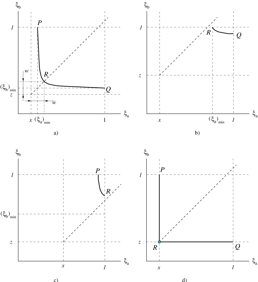
Figure 3.7: The contours of the integration over $\xi_{a}$, $\xi_{b}$ for (a,b,c) the perturbative cross-section; (d) the asymptotic and resummed cross-sections

Chapter 4 Resummation in semi-inclusive DIS: numerical results

Despite the abundance of experimental publications on SIDIS, none of them presents dependence of SIDIS observables on the variable $q_{T}$. Hence $q_{T}$-distributions, which are sensitive to the multiple parton radiation, have to be derived from the published data on less direct distributions. The $q_{T}$-distributions for some of the HERA data were reconstructed for the first time in [35, 36]. In this Chapter, I concentrate on the analysis of the $q_{T}$-distributions for the $z-$flow (3.117)

$$\frac{1}{\sigma_{tot}}\frac{d\Sigma_{z}}{dxdQ^{2}dq_{T}^{2}},$$

which can be derived from published pseudorapidity distributions for the transverse energy flow in the hCM frame [64, 65]. I will also discuss several observables, including the average value of $q_{T}^{2}$, that were measured in the production of light charged hadrons [63, 60].

Reconstruction of the $q_{T}$-dependence reveals an interesting trend in the data: namely, the average $q_{T}$ (or average $q_{T}^{2}$) increases rapidly when either $x$ or $z$ decreases. This trend is illustrated in Figs. 4.1 and 4.2. Figure 4.1 shows the average $q_{T}^{2}$ in the charged particle production for several bins of $x$ and $z$ at $28\leq Q^{2}\leq 38\mbox{\, GeV}^{2}$. The procedure of reconstruction of $\left\langle q_{T}^{2}\right\rangle$ is described in detail in Section 4.2. As can be seen from Figure 4.1, $\left\langle q_{T}^{2}\right\rangle$ in the ZEUS data sample ($\left\langle x\right\rangle=1.94\cdot 10^{-3}$) is several times higher than $\left\langle q_{T}^{2}\right\rangle$ at the same value of $\left\langle z\right\rangle$ and larger values of $\left\langle x\right\rangle$ in the E665 data sample ($\left\langle x\right\rangle=0.07-0.29$). $\left\langle q_{T}^{2}\right\rangle$ increases even faster when $\left\langle z\right\rangle$ decreases and $\left\langle x\right\rangle$ is fixed. For instance, at $\left\langle x\right\rangle=1.94\cdot 10^{-3}$ $\left\langle q_{T}^{2}\right\rangle$ increases from $3\mbox{\, GeV}^{2}$ at $\left\langle z\right\rangle=0.775$ to $82\mbox{\, GeV}^{2}$ at $\left\langle z\right\rangle=0.075$.

A similar trend is apparently present in the behavior of the quantity $\sqrt{\left\langle q_{T}^{2}\Sigma_{z}\right\rangle/\left\langle\Sigma_{z}\right\rangle},$ which was derived from the data for the distributions $d\left\langle E_{T}\right\rangle/d\eta_{cm}$ published in [65]. This quantity is shown in Figure 4.2 as a function of $Q^{2}$ and $x$. At each value of $Q^{2}$, $\sqrt{\left\langle q_{T}^{2}\Sigma_{z}\right\rangle/\left\langle\Sigma_{z}\right\rangle}$ becomes larger when $x$ decreases. Also, $\sqrt{\left\langle q_{T}^{2}\Sigma_{z}\right\rangle/\left\langle\Sigma_{z}\right\rangle}$ is roughly constant along the lines of constant $y=Q^{2}/xS_{eA}$ (i.e., the lines parallel to the kinematical boundary $y=1$). Larger values of $\sqrt{\left\langle q_{T}^{2}\Sigma_{z}\right\rangle/\left\langle\Sigma_{z}\right\rangle}$ at smaller $x$ are the evidence of “broader” distributions $d\Sigma_{z}/dq_{T}$. In the subsequent Sections, I discuss this phenomenon in the context of the $q_{T}$-resummation formalism.

In this Chapter I assume that the angle $\varphi$ is not monitored in the experiment, so that it will be integrated out in the following discussion. Correspondingly, the numerical results for $d\sigma_{BA}/(dxdzdQ^{2}dq_{T}^{2})$ will not depend on terms in Eqs. (3.62-3.63) proportional to the angular functions $A_{3}$ and $A_{4}$, which integrate to zero. The dependence on the azimuthal angle $\varphi$ is discussed in more detail in Chapter 5.

Figure 4.1: The average $q_{T}^{2}$ as a function of $x$ and $z$ in the charged particle production at $Q^{2}=28-38\mbox{\, GeV}^{2}$. The data points are extracted from published distributions $\langle p_{T}^{2}\rangle$ vs. $x_{F}$ [63, 60] using the method described in Section 4.2.

Figure 4.2: $\sqrt{\left\langle q_{T}^{2}\Sigma_{z}\right\rangle/\left\langle\Sigma_{z}\right\rangle}$ reconstructed from distributions $d\left\langle E_{T}\right\rangle/d\eta_{cm}$ in bins of $x$ and $Q^{2}$ [65].

4.1 Energy flows

4.1.1 General remarks

As was discussed at length in Subsection 3.4.2, knowledge of the resummed SIDIS cross section can be used to predict the pseudorapidity spectrum of the transverse energy flow in the hadron Breit frame or the hCM frame. It is advantageous to study the energy flows, because they are less dependent on the specifics of the final-state fragmentation of the scattered partons into the observed hadrons. I therefore start the presentation of the numerical results with the comparison of the resummation formalism to the experimentally measured pseudorapidity distributions for the transverse energy flow in the hCM frame.

I consider the data on $d\left\langle E_{T}\right\rangle/d\eta_{cm}$ which has been published in [64, 65]. I consider seven bins of $x$ and $Q$ from [64] ($10\leq\left\langle Q^{2}\right\rangle\leq 50\,\,\mbox{\, GeV}^{2}$, $3.7\cdot 10^{-4}\leq\left\langle x\right\rangle\leq 4.9\cdot 10^{-3}$) and two sets of bins of $x$ and $Q$ from [65] (“low-$Q^{2}$” set covering $13.1<\langle Q^{2}\rangle<70.2\mbox{\, GeV}^{2}$, $8\times 10^{-5}<\langle x\rangle<7\times 10^{-3}$ and “high-$Q^{2}$” set covering $175<\langle Q^{2}\rangle<2200\mbox{\, GeV}^{2}$ and $0.0043<\langle x\rangle<0.11$).

The experimental distributions $d\left\langle E_{T}\right\rangle/d\eta_{cm}$ at a fixed value of $W^{2}=Q^{2}(1-x)/x$ can be converted into the distributions $d\Sigma_{z}/dq_{T}$ using Eqs. (3.25,3.119):

$$q_{T}=We^{-\eta_{cm}}$$ (4.1)

and

$$\frac{d\Sigma_{z}}{dxdQ^{2}dq_{T}}=\frac{1}{q_{T}^{2}}\frac{d\langle E_{T}\rangle}{dxdQ^{2}d\eta_{cm}}.$$ (4.2)

The “derived” data for $d\Sigma_{z}/(dxdQ^{2}dq^{2}_{T})$ can be compared with the resummed $z$-flow (3.123), which is calculated as

$$\frac{d\Sigma_{z}}{dxdQ^{2}dq^{2}_{T}}=\frac{\pi}{S_{eA}}\sigma_{0}F_{l}\left(1+\cosh^{2}\psi\right)\int\frac{d^{2}b}{(2\pi)^{2}}e^{i\vec{q}_{T}\cdot\vec{b}}\widetilde{W}_{z}(b,Q,x)+Y_{z},$$ (4.3)

where

$$\widetilde{W}_{z}(b,Q,x)=\sum_{j}e_{j}^{2}{\mathcal{C}}^{out}_{z}\,e^{-S_{z}(b,Q,x)}\,({\mathcal{C}}_{ja}^{in}\otimes F_{a/A})(x,b_{*},\mu).$$ (4.4)

The Sudakov factor $S_{z}$ in Eq. (4.4) is

$$S_{z}(b,Q,x)=S^{P}(b_{*},Q,x)+S^{NP}_{z}(b,Q,x),$$

where the perturbative part $S^{P}$ is given by Eq. (3.93), and a realistic parametrization of the nonperturbative part $S_{z}^{NP}(b,Q,x)$ can be obtained by comparison with experimental data at low and intermediate values of $Q$, especially with the measured pseudorapidity distributions at $Q\approx 3-20$ GeV. At high $Q$, we expect the data to be dominated by the perturbatively calculable parton radiation and be less sensitive to the nonperturbative effects incorporated in $S_{z}^{NP}(b,Q,x)$. According to the renormalization group invariance argument, $S_{z}^{NP}$ includes a part that is proportional to $\ln Q$:

$$S^{NP}_{z}(b,Q,x)=g^{(1)}(b,x)+g^{(2)}(b,x)\log\frac{Q}{Q_{0}},$$ (4.5)

where the parameter $Q_{0}\approx 1\mbox{\, GeV}^{-1}$ prevents $\ln{Q/Q_{0}}$ from being negative in the region of validity of PQCD. In the following analysis, I use two parametrizations of $S_{z}^{NP}(b,Q,x),$ which I will call parametrizations 1 and 2.

• Parametrization 1   was   proposed   in our paper [35] with D. Stump and C.-P. Yuan based on the analysis of the data in Ref. [64]:

  $$S^{NP}_{z}(b,Q,x)=b^{2}\left\{g^{(1)}(x)+\frac{1}{2}\Bigl{(}\left.g^{(2)}(b,Q)\right|_{DY}+\left.g^{(2)}\right|_{e^{+}e^{-}}(b,Q)\Bigr{)}\right\},$$ (4.6)

  where $\left.g^{(2)}(b,Q)\right|_{DY}$ and $\left.g^{(2)}(b,Q)\right|_{e^{+}e^{-}}$ are $Q$-dependent terms in the nonperturbative Sudakov factors in Drell-Yan process and $e^{+}e^{-}$ hadroproduction. The parametrization of the function $g^{(2)}(b,Q)$ in Eq. (4.6) is suggested by the crossing symmetry between SIDIS, the Drell-Yan process and $e^{+}e^{-}$ hadroproduction. Due to this symmetry, the functions $g^{(2)}(b,Q)$ in these processes may be related as [33]

  $$\left.g^{(2)}(b,Q)\right|_{SIDIS}=\frac{1}{2}\Bigl{(}\left.g^{(2)}(b,Q)\right|_{DY}+\left.g^{(2)}(b,Q)\right|_{e^{+}e^{-}}\Bigr{)}.$$ (4.7)

  If the relationship (4.7) is true, then the function $g^{(2)}(b,Q)$ in SIDIS is completely known once parametrizations for the functions $g^{(2)}(b,Q)$ in the Drell-Yan and $g^{(2)}(b,Q)$ in $e^{+}e^{-}$ hadroproduction processes are available. In practice, the only known parametrization of the nonperturbative Sudakov factor in the $e^{+}e^{-}$ hadroproduction was obtained in Ref. [19] by fitting the resummation formula to the data at $Q=27$ GeV. Most of the $\left\langle E_{T}\right\rangle$ data from HERA correspond to significantly smaller values of $Q$, where the usage of the parametrization [19] is questionable. In addition, the known parametrizations of the nonperturbative Sudakov factors for the Drell-Yan [22, 24, 25, 26, 27] and $e^{+}e^{-}$ hadroproduction [19] processes correspond to slightly different scale choices:

  $$C_{1}=b_{0},\quad C_{2}=1$$ (4.8)

  and

  $$C_{1}=b_{0},\quad C_{2}=e^{-3/4},$$ (4.9)

  respectively. Therefore, the known functions $\left.g^{(2)}\right|_{DY}(b)$ and $\left.g^{(2)}\right|_{e^{+}e^{-}}(b)$ are not 100% compatible and in principle should not be combined to obtain $g^{(2)}(b)$ for SIDIS. In the numerical calculation, I have used the functions $\left.g^{(2)}(b)\right|_{DY}$ from [22] and $\left.g^{(2)}(b)\right|_{e^{+}e^{-}}$ from [17], despite the fact that $\left.g^{(2)}(b)\right|_{DY}$ was fitted to Drell-Yan data using a different $C_{2}$ value than in $\left.g^{(2)}(b)\right|_{e^{+}e^{-}}$. Explicitly, the $Q$-dependent part $g^{(2)}(b,Q)$ in Eq. (4.6) is

  $$g^{(2)}(b,Q)=\frac{1}{2}b^{2}\Biggl{(}0.48\log(\frac{Q}{2Q_{0}})+5.32C_{F}\log\Bigl{(}\frac{b}{b_{*}}\Bigr{)}\log\Bigl{(}\frac{C_{2}Q}{C_{1}Q_{0}}\Bigr{)}\Biggr{)}.$$ (4.10)

  In Eq. (4.10), the constants are $C_{1}=2e^{-\gamma_{E}},\,\,C_{2}=e^{-3/4},Q_{0}=1\,\,\mbox{\, GeV}$. The variable $b_{*}$ is given by Eq. (3.111), with $b_{max}=0.5\,\,\mbox{\, GeV}^{-1}$.

  The functional form of $g^{(1)}(b,x)$ in terms of $b$ and $x$ was parametrized as

  $$g^{(1)}(b,x)=(-4.58+\frac{0.58}{\sqrt{x}})b^{2},$$ (4.11)

  where the numerical coefficients were determined by fitting the experimental data. These data cover a limited region of $x$ and $Q^{2}$ ($10\leq Q^{2}\leq 50\,\,\mbox{\, GeV}^{2}$, $3.7\cdot 10^{-4}\leq x\leq 4.9\cdot 10^{-3}$ ), so that the parametrization 1 should not be used away from this region. Also, the dependence of $S_{z}^{NP}(b,Q,x)$ on $Q$ cannot be determined reliably using exclusively the data from Ref. [64], since all pseudorapidity distributions in this publication are presented in a small range of $Q\approx 2-6$ GeV. This circumstance motivated us to model the $Q$-dependent terms in the parametrization 1 by using the crossing relationship (4.7) instead of trying to find these terms from the comparison with the data.

• Parametrization 2 overcomes several shortcomings of the parametrization 1. The parametrization 2 was proposed in [36], where the analysis of Ref. [35] was repeated using the latest and more comprehensive data on the transverse energy flow [65]. From our analysis, we found that the data from Refs. [64, 65] are consistent with the following representative parametrization of the nonperturbative Sudakov factor:

  $$S^{NP}_{z}(b,Q,x)=b^{2}\,\left(0.013\frac{(1-x)^{3}}{x}+0.19\ln{\frac{Q}{Q_{0}}}+C\right),$$ (4.12)

  where the parameter $Q_{0}$ is fixed to be 2 GeV to prevent $\ln{Q/Q_{0}}$ from being negative in the region of validity of PQCD, and where we set $C=0$ for reasons explained later.

  The H1 Collaboration presented pseudorapidity distributions of the transverse energy flow for $Q^{2}$ up to $2200\mbox{\, GeV}^{2}$. However, the data at such high $Q^{2}$ is rather insensitive to the nonperturbative dynamics because of the poor resolution of the H1 detector in the region of large $Q^{2}$ and $\eta_{cm}$. Thus the H1 data at very high $Q^{2}$ is not informative about the $Q^{2}$-dependence of $S_{z}^{NP}(b,Q,x)$ either. Fortunately, the H1 Collaboration presented distributions in two bins at intermediate values of $\langle Q^{2}\rangle$, namely $\langle Q^{2}\rangle=59.4\mbox{\, GeV}^{2}$ and $\langle Q^{2}\rangle=70.2\mbox{\, GeV}^{2}$. Together with the data from Refs. [64, 65] at lower values of $Q$, these distributions provide the first direct tests of the $Q^{2}$-dependence of $S_{z}^{NP}(b,Q,x)$. Therefore the parametrization 2 of $S_{z}^{NP}(b,Q,x)$ includes a numerical value for the coefficient of $\ln Q/Q_{0}$, which yields reasonable agreement with all of the analyzed data. The resulting value for this coefficient differs noticeably from its model expression in the parametrization 1. However, we should not draw too strong a conclusion from this difference, because it might be caused by ambiguities in the separation of $Q^{2}$ dependence and $x$ dependence in the existing data. To draw a strong conclusion about the crossing symmetry model, experimental pseudorapidity distributions in a larger range of $x$ at intermediate values of $Q^{2}$, as well as improvements in the knowledge of the nonperturbative Sudakov factor in the $e^{+}e^{-}$-hadroproduction will be needed.

4.1.2 Comparison with the data

The numerical results below were obtained using the parameters of the HERA electron-proton collider. The energies of the proton and electron beams are taken to be equal to 820 and 27.5 GeV, respectively. All calculations were performed using CTEQ5M1 parton distribution functions [90] and the parametrization 2 of the nonperturbative Sudakov function $S_{z}^{NP}$ (Eq. (4.12)), unless stated otherwise. The theoretical results in Figs. 4.3-4.5 were obtained using the kinematical correction to the asymptotic and resummed cross-sections at non-zero $q_{T}$, which was discussed in Subsection 3.6.2. The factorization and renormalization scales of the perturbative and asymptotic pieces are all set equal to $\mu=Q$. The resummed piece was calculated using $C_{1}=b_{0},\,C_{2}=1,\,\mu=b_{0}/b$, where $b_{0}\equiv 2e^{-\gamma_{E}}$.

In Fig. 4.3, I present the comparison of the existing data from [64] in one of the bins of $x$ and $Q^{2}$ ($\langle x\rangle=0.0049,\,\,\langle Q^{2}\rangle=32.6\,\,\mbox{\, GeV}^{2}$) with the NLO perturbative and resummed $z$-flows. Figure 4.3 demonstrates two important aspects of the NLO $q_{T}$ distribution (dashed curve): namely, the NLO $z$-flow exceeds the data at small $q_{T}$ and is below the data at $q_{T}\geq Q$. In fact, the deficit of the NLO prediction in comparison with the data at medium and large $q_{T}$ ($q_{T}\geq 5\,\,\mbox{\, GeV}$) is present in the entire region of $x$ and $Q^{2}$ that was studied.

As I discussed in Section 3.6, one can trust the resummed calculation only for reasonably small values of $q_{T}/Q$. For large values of $q_{T}$, the fixed-order perturbative result is more reliable. This means that the NLO resummation formalism will not give an accurate description of the data for $q_{T}\gg Q$ due to the small magnitude of the NLO perturbative $z$-flow in this region.

Figure 4.3: Comparison of the NLO perturbative and resummed expressions for the $z$-flow distribution with the existing experimental data from HERA [64]. The data is for $\langle x\rangle=0.0049,\,\,\langle Q^{2}\rangle=32.6\mbox{\, GeV}^{2}$. The resummed curve is calculated using the parametrization 1 of $S_{z}^{NP}.$ CTEQ4M PDFs [91] were used.

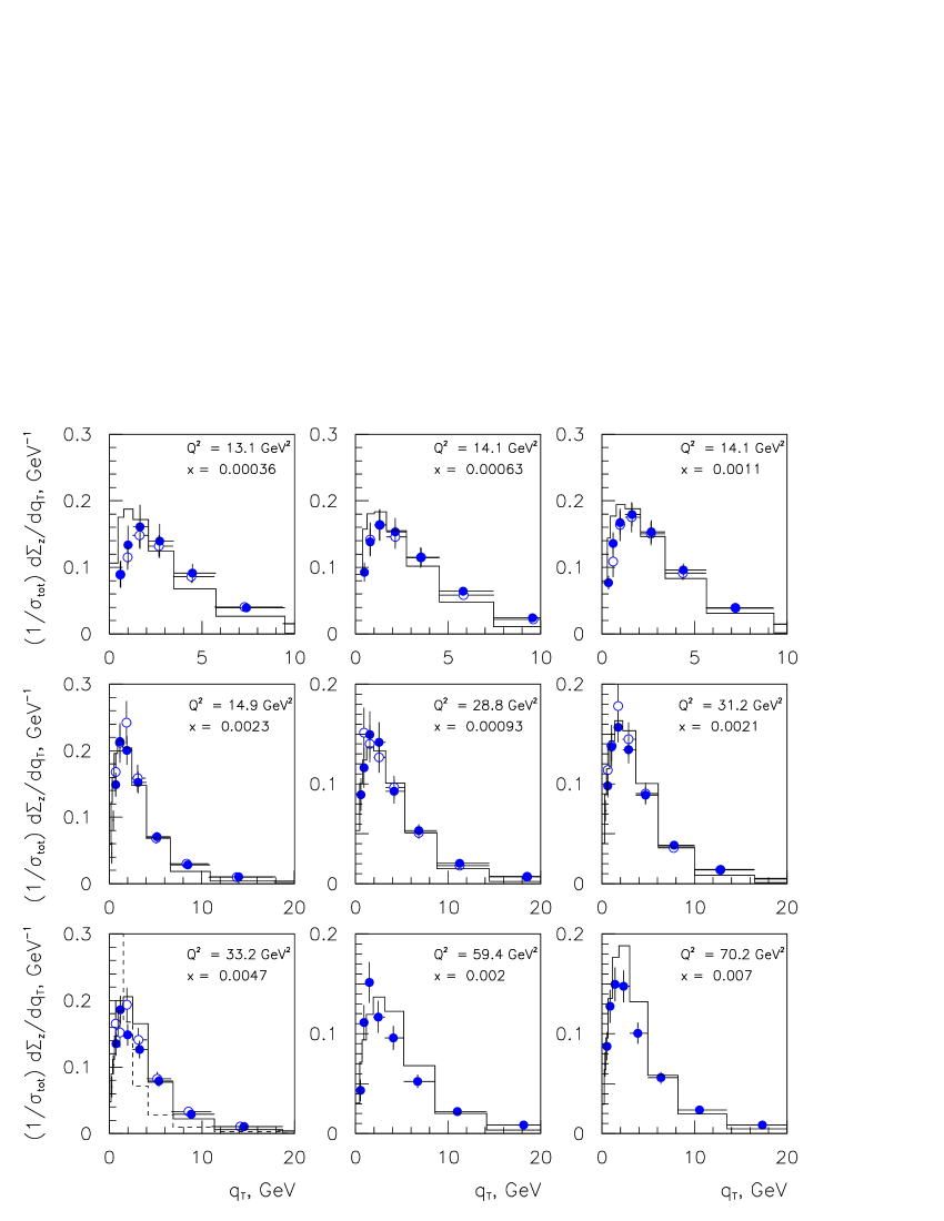
Figure 4.4: Comparison of the resummed $z$-flow (solid curve) in the current region of the hCM frame with the data in the low-$Q^{2}$ bins from Refs. [65] (filled circles) and [64] (empty circles). For the bin with $\langle Q^{2}\rangle=33.2\mbox{\, GeV}^{2}$ and $\langle x\rangle=0.0047$, the fixed-order ${\mathcal{O}}(\alpha_{S})$ contribution for the factorization scale $\mu=Q$ is shown as the dashed curve.

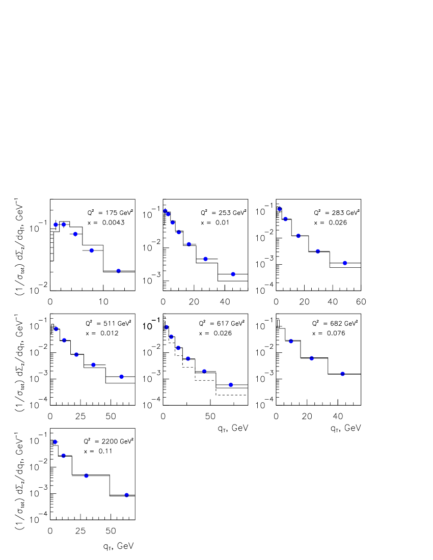
Figure 4.5: Comparison of the resummed $z$-flow in the current region of the hCM frame with the data in the high-$Q^{2}$ bins from Ref. [65]. For the bin with $\langle Q^{2}\rangle=617\mbox{\, GeV}^{2}$ and $\langle x\rangle=0.026$, the ${\mathcal{O}}(\alpha_{S})$ contribution for $\mu_{F}=Q$ is shown as a dashed curve.

The excess of the data over the NLO calculation at large $q_{T}$ (cf. Figs. 4.3-4.5) can be interpreted as a signature of other intensive hadroproduction mechanisms at hCM pseudorapidities $\eta_{cm}\leq 2$. A discussion of the cross-sections in this pseudorapidity region is beyond the scope of this thesis. There exist several possible explanations of the data in this region, for instance, the enhancement of the cross-section due to BFKL showering [56] or resolved photon contributions [68, 71]. It is clear, however, that better agreement between the data and the theory, in a wider range of $\eta_{cm}$, will be achieved when next-to-next-to-leading order contributions, like the ones contributing to (2+1) jet production [69], are taken into account.

On the other hand, Figs. 4.3-4.5 illustrate that the resummed $z$-flow is in better agreement with the data, over a wide range of $q_{T}/Q$, but also lies below the data if $q_{T}/Q$ significantly exceeds unity. The better consistency between the resummed $z$-flow and the data suggests that the resummed $z$-flow should be used up to values of $q_{T}/Q\sim 1-4$, i.e., without switching to the fixed-order expression. This procedure was followed in the derivation of our numerical results.

Let us discuss the features of the data presented in Figs. 4.4 and 4.5. First, the data in the low-$Q^{2}$ bins is significantly influenced by nonperturbative effects and therefore is sensitive to the details of the parametrization of $S^{NP}_{z}(b,Q,x)$. This feature can be seen from the abundance of data points around the maximum of the $q_{T}$-distribution, where the shape is mainly determined by $S^{NP}_{z}(b,Q,x)$. Also, the low-$Q^{2}$ data from HERA is characterized by small values of $x$, between $10^{-4}$ and $10^{-2}$. For the theory to be consistent with the data from Ref. [64] in this range of $x$, the nonperturbative Sudakov factor must increase rapidly as $x\rightarrow 0$, at least as $1/\sqrt{x}$. Such $x$-dependence is implemented in the parametrization 1 of $S_{z}^{NP}.$ In our newer analysis, we found that growth of $S^{NP}_{z}(b,Q,x)$ as $1/x$ at small $x$ is in better agreement with the more recent data from [65].

Second, the data in the high-$Q^{2}$ bins of Fig. 4.5 shows a behavior that is qualitatively different from Fig. 4.4. In the region covered by the experimental data points, the $q_{T}$ distribution is a monotonically decreasing function of $q_{T}$, which shows good agreement with the resummed $z$-flow over a significant range of $q_{T}$. In the region $q_{T}<10$ GeV, i.e., where the maximum of the $q_{T}$ distribution is located and where nonperturbative effects are important, the experimental $q_{T}$-bins are too large to provide any information about the shape of $d\Sigma_{z}/dq_{T}$. Thus, as mentioned earlier, the published high-$Q^{2}$ $z$-flow data from Ref. [65] is not sensitive to the dynamics described by the nonperturbative Sudakov factor $S^{NP}_{z}(b,Q,x)$.

A third comment is that most of the high-$Q^{2}$ data points in Fig. 4.5 correspond to $\langle x\rangle>10^{-2}$. If the resolution of the H1 measurements at high $Q^{2}$ were better in the small-$q_{T}$ region, then the high-$Q^{2}$ data would also reveal the behavior of $S^{NP}_{z}(b,Q,x)$ at large $x$. But, as mentioned before, the published data in the high-$Q^{2}$ bins are not very sensitive to the shape of the $z$-flow at small $q_{T}$. Therefore it is not possible to impose any constraints on $S^{NP}_{z}(b,Q,x)$ at large values of $x$, except that it should be positive, $S^{NP}_{z}(b,Q,x)>0$. For this reason we have chosen the $x$-dependent part of $S^{NP}_{z}(b,Q,x)$ in the parametrization 2 such that $S^{NP}_{z}(b,Q,x)$ grows approximately as $1/x$ as $x\rightarrow 0$ and is positive for all $x$. For the same reason, we chose $C=0$ in the parametrization 2. Although the most general parametrization of $S_{z}^{NP}(b,Q,x)$ can have $C\neq 0$, the current data cannot distinguish between the parametrization 2 with $C=0$ and $C\neq 0$, as long as the value of $C$ is not very large.

Finally, Fig. 4.6 shows the results of our calculation presented as the hCM pseudorapidity distributions of the transverse energy flow $\langle E_{T}\rangle$. This quantity is obtained by the transformation (3.119). The small-$q_{T}$ region, where the resummation formalism is valid, corresponds to large pseudorapidities. In this region, the agreement between our calculation and the data is good. At smaller pseudorapidities (larger $q_{T}$), one sees the above-mentioned excess of the data over the perturbative NLO calculation. In the $\langle E_{T}\rangle$ vs. $\eta_{cm}$ plot, this excess is magnified because of the factor $q_{T}^{2}$ in the transformation (4.2).

4.1.3 How trustworthy is the resummed $z$-flow at large $q_{T}$?

As noted earlier, the ${\mathcal{O}}(\alpha_{S})$ fixed-order $z$-flow is much larger than the data in the region $q_{T}/Q\ll 1$ and smaller than the data in the region $q_{T}/Q\gtrsim 1$. In the small-$q_{T}$ region, the resummed $z$-flow is, by its construction, more reliable than the fixed-order result. In the large-$q_{T}$ region, the resummed $z$-flow, with the kinematical correction (3.141) included, is also in better agreement with the data than the fixed-order calculation. But theoretically, the resummed $z$-flow at large $q_{T}/Q$ is not absolutely trustworthy, because it does not include those parts of the fixed-order $z$-flow that are subleading in the limit $q_{T}\rightarrow 0$, but which might be important at large $q_{T}$. If the NLO result were in a good agreement with the data at large $q_{T}$, it would be justified to consider it a more reliable prediction in this region. But since the ${\mathcal{O}}(\alpha_{S})$ contribution is systematically smaller than the data, higher-order corrections are presumably necessary in order to describe the region $q_{T}\gtrsim Q$ reliably.

A systematic approach for improving the theoretical description of the large-$q_{T}$ region would require inclusion of the complete ${\mathcal{O}}(\alpha_{S}^{2})$ terms in both the fixed-order and resummed $z$-flows. But because such a calculation is not available, it might be beneficial to use the resummed $z$-flow as a better theoretical prediction both in the region $q_{T}/Q\ll 1$, where application of the resummation formalism is fully justified, and for $q_{T}$ up to several units of $Q$, where the resummed $z$-flow agrees with the data better than the fixed-order one. Then the use of the resummed $q_{T}$-distributions of the $z$-flow will provide more reliable predictions for other observables relevant to the SIDIS process.
As an example, resummation can improve the reliability of the theoretical prediction for the azimuthal asymmetry of the $z$-flow. The $b$-space resummation formalism affects only the coefficient ${\,}^{1}V_{zA}$ of the angular function $A_{1}(\psi,\varphi)$. This coefficient is the one that dominates the $\varphi$-integrated $z$-flow in the small-$q_{T}$ region, where the energy flow is the most intense. On the other hand, the main goal of the measurement of angular asymmetries is to study structure functions other than ${\,}^{1}V_{zA}$, e.g., those corresponding to the angular functions $A_{3}(\psi,\varphi)=-\cos\varphi\sinh 2\psi$ and $A_{4}(\psi,\varphi)=\cos 2\varphi\sinh^{2}\psi$. By using a better approximation for the coefficient ${\,}^{1}{V}_{zA}$, it is possible to measure the coefficients ${\,}^{3,4}V_{zA}$ more reliably. Conversely, by knowing that the all-order resummation effects are important in the region of small $q_{T}$ and by concentrating on the region where $q_{T}$ is of the order $Q$ or larger, one may find angular asymmetries that are well approximated in the lowest orders of PQCD. The impact of resummation on the angular asymmetries is discussed in more detail in Chapter 5.

Figure 4.6: The hCM pseudorapidity distributions of the transverse energy flow in the current fragmentation region. The data are from [64]. CTEQ4M PDFs and the parametrization 1 of $S_{z}^{NP}$ were used.

4.2 Normalized distributions of charged particle production

Let us now turn to the discussion of particle multiplicities. Although the resummation formalism, as outlined in Chapter 3, can describe the cross section for any massless final-state particle (provided that the fragmentation functions for this particle are known), in this Section I will concentrate on distributions of the charged particle multiplicity, defined as

$$\frac{1}{\sigma_{tot}}\frac{d\sigma(A+e\rightarrow h^{\pm}+e+X)}{d\Theta}.$$ (4.13)

Here $\Theta$ is some kinematical variable, such as the variable $q_{T}^{2}$ in Eq. (3.6), the transverse momentum $p_{T}$ of the final-state charged particle in the hCM frame, or the Feynman variable $x_{F}$,

$$x_{F}\equiv\frac{2p_{B,cm}^{z}}{W}=z\left(1-\frac{q_{T}^{2}}{W^{2}}\right).$$ (4.14)

Our calculation assumes that the charged particles registered in the detector are mostly charged pions, kaons and protons. Therefore the cross section for charged particle production can be calculated using (3.60) with the replacement of the fragmentation functions $D_{B/b}(\xi_{b},\mu)$ by

$$D_{h^{\pm}/b}(\xi_{b},\mu)\equiv\sum_{B=\pi^{\pm},K^{\pm},p,\bar{p}}D_{B/b}(\xi_{b},\mu).$$ (4.15)

The fragmentation functions $D_{B/b}(\xi_{b},\mu)$ are known reasonably well only for $\xi_{b}\gtrsim 0.05-0.1$ [87, 88, 89]. Thus, the formalism presented here is applicable to the production of charged particles with sufficiently large energies, i.e., for $z\gtrsim 0.05$.

Certain experimental distributions are readily available from the literature [59, 60, 62, 63], such as $d\sigma/dp_{T}$, $d\sigma/dx_{F}$, as well as distributions for the average transverse momentum $\langle p_{T}^{2}\rangle$. However, the “experimental” $q_{T}$ distributions must currently be derived from pseudorapidity distributions by using Eq. (3.25). Although the distributions $d\sigma/dp_{T}$ and $\langle p_{T}^{2}\rangle$ are quite sensitive to resummation effects, they cannot be interpreted as easily as the distributions $d\sigma/dq_{T}$, primarily because the distributions $d\sigma/dp_{T}$ and $\langle p_{T}^{2}\rangle$ mix resummation effects at small values of $q_{T}$ with perturbative contributions from the region $q_{T}/Q\gtrsim 1$. The most straightforward way to study the effects of multiple parton radiation would be to consider the $q_{T}$ (or pseudorapidity) distributions that satisfy the additional requirement $z>0.05-0.1$ and that are organized in small bins of $Q^{2}$ and $x$. Unfortunately, such distributions have not been published yet. Although Ref. [59] presents distributions $d\sigma(p+e\rightarrow h^{\pm}+e+X)/d\eta_{cm}$ for some values of $x$ and $Q^{2}$, these distributions are integrated over the full range of $z$. Therefore, they are sensitive to the uncertainties in fragmentation functions, mass effects, and contributions from diffractive scattering.

Because the experimental $q_{T}$ distributions are unavailable, we have decided to undertake a simpler analysis than the one presented for the energy flow. Our goal here is to understand how the multiple parton radiation could affect various aspects of charged particle production. For this purpose we focused our attention on data from the ZEUS Collaboration [60], which presents the charged particle multiplicity in a phase-space region characterized by the mean values $\langle W\rangle=120\mbox{\, GeV}$, $\langle Q^{2}\rangle=28\mbox{\, GeV}^{2}$, and the additional constraint $z>0.05$. These values of $\langle W\rangle$ and $\langle Q^{2}\rangle$ translate into an average value of $x=1.94\times 10^{-3}$. A simple model for nonperturbative effects at small $q_{T}$ will demonstrate that resummation describes qualitative features of this set of experimental data better than the fixed-order calculation.

In all of the cases presented, the strategy is to compare the resummed multiplicity to that from the next-to-leading order calculation. In the numerical analysis, the multiplicity was calculated using the CTEQ5M1 PDFs [90] and the FFs from [88]. For the resummed multiplicity, the “canonical” combination $C_{1}=b_{0},\,C_{2}=1,\,\mu=b_{0}/b$ was used. The NLO cross section was calculated according to Eq. (3.85), for the factorization scale $\mu=Q$. As explained in detail in Section 3.4.1, the integration of the NLO term over $q_{T}$ is done separately over the regions $0\leq q_{T}\leq q_{T}^{S}$ and $q_{T}>q_{T}^{S}$, where $q_{T}^{S}$ is a particular type of a phase space slicing parameter. The final results should not depend on the exact value of $q_{T}^{S}$ provided that it is chosen in the region where the ${\mathcal{O}}(\alpha_{S})$ part of the next-to-leading-logarithmic expansion (3.73) approximates well the exact NLO cross section. In practical calculations, $q_{T}^{S}$ cannot be chosen to be too small, because the numerical calculation becomes unstable due to large cancellations between the integrals over the regions $0\leq q_{T}\leq q_{T}^{S}$ and $q_{T}\geq q_{T}^{S}$. The NLO prediction for the integrated charged particle multiplicity $\sigma_{chgd}/\sigma_{tot}$ at $\langle W\rangle=120\mbox{\, GeV}$, $\langle Q^{2}\rangle=28\mbox{\, GeV}^{2}$ is practically independent of $q_{T}^{S}$ in the region $1\lesssim q_{T}^{S}\lesssim 2.5$ GeV (cf. Figure 4.7). The NLO distributions shown in the subsequent Figures were calculated for $q_{T}^{S}=1.2$ GeV, which lies within the range of stability of $\sigma^{chgd}/\sigma_{tot}$. As in the case of the $z$-flow, the resummed charged particle multiplicity may suffer from matching ambiguities at $q_{T}/Q\sim 1$.

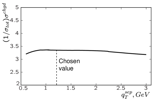
Figure 4.7: The dependence of the ${\mathcal{O}}(\alpha_{S})$ prediction for the total charged particle multiplicity on the value of the separation scale $q_{T}^{S}$. The calculation is done for $\langle W\rangle=120\mbox{\, GeV},\,\,\langle Q^{2}\rangle=28\mbox{\, GeV}^{2}$.

In Section 4.1, we found that the resummed $z$-flow is in better agreement with the experimental distributions than the NLO $z$-flow, for the whole range $q_{T}/Q\lesssim 2-4$. That result suggests that it might be preferable to use the resummed $z$-flow in the whole range $q_{T}/Q\lesssim 2-4$ as a better theoretical prediction, until the ${\mathcal{O}}(\alpha_{S}^{2})$ prediction for the $z$-flow in the region $q_{T}/Q\gtrsim 1$ becomes available. In the case of the charged particle multiplicity, the resummed cross section, which is calculated according to the formula

$$\frac{d\sigma_{BA}}{dxdzdQ^{2}dq_{T}^{2}}=\frac{\sigma_{0}F_{l}}{\pi S_{eA}}\int\frac{d^{2}b}{(2\pi)^{2}}e^{i\vec{q}_{T}\cdot\vec{b}}\widetilde{W}_{BA}(b,x,z,Q)+Y_{BA},$$ (4.17)

overestimates the experimentally measured rate for the production of charged particles with $p_{T}>2$ GeV. This discrepancy indicates that the resummed cross section in the region $q_{T}/Q\gtrsim 1$ is too high, so that switching to the perturbative cross section in this region is in fact required. Therefore, we have chosen to use the resummed cross section for $q_{T}\leq 5$ GeV and switch to the next-to-leading order cross section for $q_{T}\geq 5$ GeV.

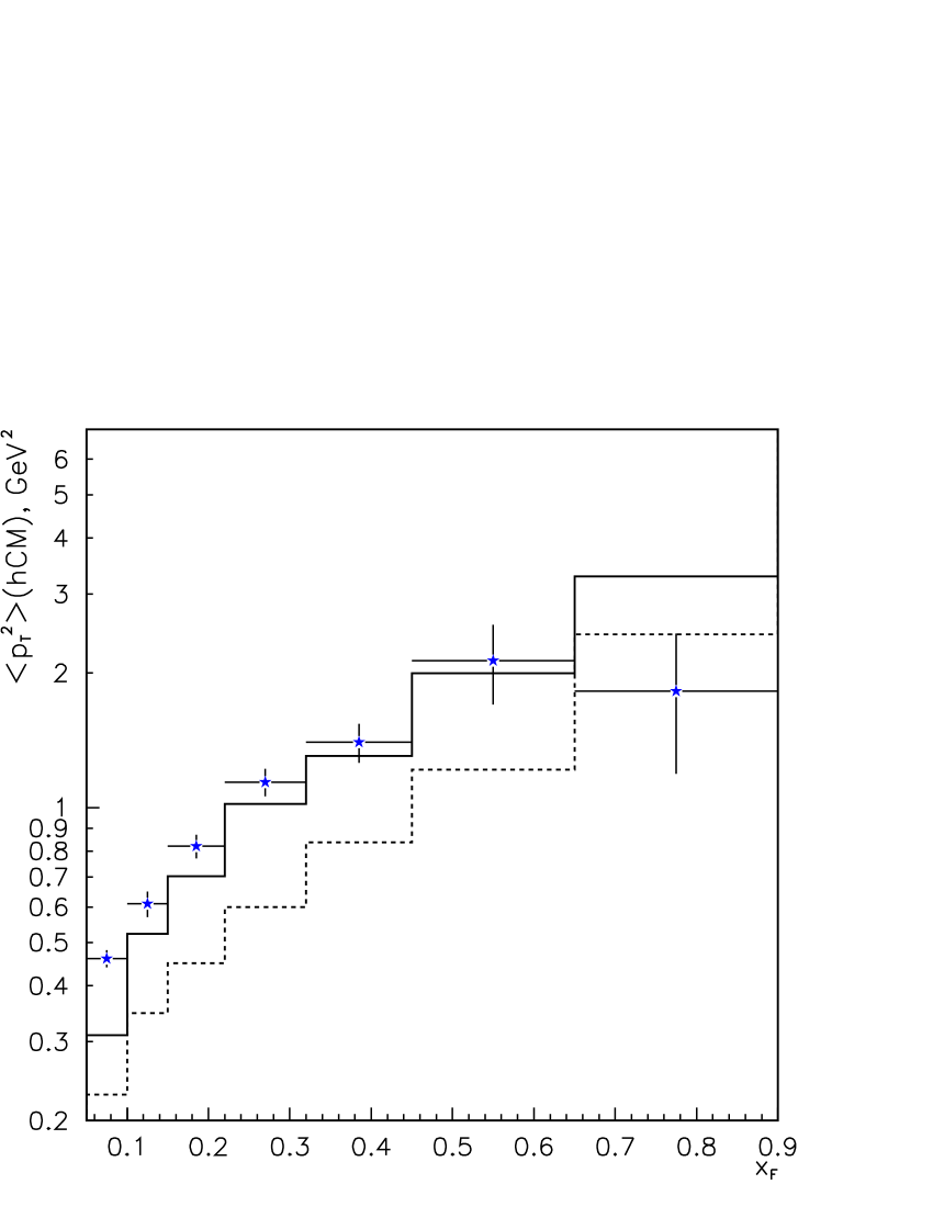
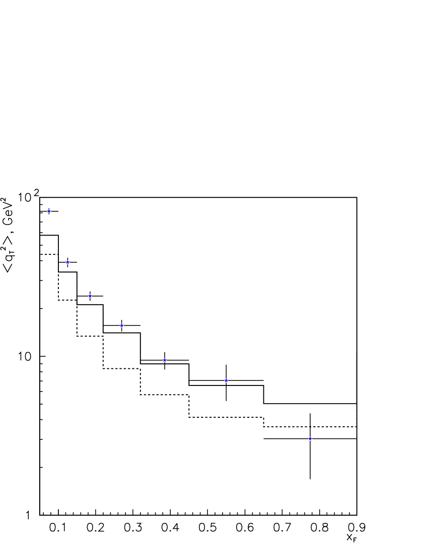
a)                                                              b)

Figure 4.8: The distributions (a) $\langle p_{T}^{2}\rangle$ vs. $x_{F}$ and (b) $\langle q_{T}^{2}\rangle$ vs. $x_{F}$ for the charged particle multiplicity at $\langle W\rangle=120\mbox{\, GeV},\,\,\langle Q^{2}\rangle=28\mbox{\, GeV}^{2}$. The experimental points for the distribution $\langle p_{T}^{2}\rangle$ vs. $x_{F}$ are from Fig. 3c of Ref. [60]. The “experimental” points for the distribution $\langle q_{T}^{2}\rangle$ vs. $x_{F}$ are derived using Eq. (4.19). The solid and dashed curves correspond to the resummed and NLO ($\mu=Q$) multiplicity, respectively.

As in the case of the $z$-flow, the shape of the $q_{T}$ distribution for the charged particle multiplicity at small values of $q_{T}$ depends strongly on the unknown nonperturbative Sudakov factor $S^{NP}(b,Q,x,z)$. For the purposes of this study, we introduced a preliminary representative parametrization of the nonperturbative Sudakov factor for the fixed values of $x=1.94\times 10^{-3}$ and $Q^{2}=28\mbox{\, GeV}^{2}$, i.e., the values that coincide with the average values of $x$ and $Q^{2}$ in [60]. This $z$-dependent parametrization is

$$S^{NP}\left(b,Q^{2}=28\mbox{\, GeV}^{2},x=1.94\times 10^{-3},z\right)=b^{2}\left(0.18+0.8\frac{(1-z)^{3}}{z^{1.4}}\right).$$ (4.18)

Since the ZEUS Collaboration did not publish pseudorapidity distributions for the charged particle multiplicity $(1/\sigma_{tot})d\sigma/d\eta_{cm}$ in bins of varying $z$, we had to deduce information about the $z$-dependence of $S^{NP}$ from the less direct distribution of $\langle p_{T}^{2}\rangle$ vs. $x_{F}$ presented in Fig. 3c of [60]. This distribution, known as a “seagull” for its characteristic shape (Fig. 4.8a), can be converted into the more illustrative distribution of $\langle q_{T}^{2}\rangle$ vs. $x_{F}$ (Fig. 4.8b). Since the major portion of the registered events comes from the region $q_{T}^{2}/W^{2}\ll 1$, or $x_{F}\approx z$, a first estimate of the experimental data points for the distribution of $\langle q_{T}^{2}\rangle$ vs. $x_{F}$ can be obtained by assuming that

$$\langle q_{T}^{2}\rangle\approx\frac{\langle p_{T}^{2}\rangle}{\langle z\rangle^{2}}\approx\frac{\langle p_{T}^{2}\rangle}{\langle x_{F}\rangle^{2}},$$ (4.19)

where $\langle x_{F}\rangle$ denotes central values of $x_{F}$ in each bin in Fig. 4.8a. We refer to the resulting values as “derived data”.

Note that the shapes of $\langle p_{T}^{2}\rangle$ vs. $x_{F}$ and $\langle q_{T}^{2}\rangle$ vs. $x_{F}$ are quite different. The transformation from Fig. 4.8a to Fig. 4.8b shows immediately that the wing-like shape of the distribution of $\langle p_{T}^{2}\rangle$ vs. $x_{F}$ should be attributed to a purely kinematical effect, namely an extra factor $1/z^{2}$ which is absent in the distribution of $\langle q_{T}^{2}\rangle$ vs. $x_{F}$. Once this extra factor is removed, we see from Fig. 4.8b that $\langle q_{T}^{2}\rangle$ increases monotonically and rapidly as $z$ approaches zero. In other words, the $q_{T}$ distribution broadens rapidly when $z$ decreases. This behavior is approximately realized by the simple $z$-dependent nonperturbative Sudakov factor $S^{NP}(b,Q,x,z)$ given in Eq. (4.18).

Figure 4.9: The dependence of the charged particle multiplicity on the transverse momentum $p_{T}$ of the observed particles in the hCM frame. The data points are from [60]. The solid and dashed curves correspond to the resummed and NLO multiplicities, respectively.

The parametrization of $S^{NP}(b,Q,x,z)$ was chosen to maximize the agreement between the resummed distribution of $\langle q_{T}^{2}\rangle$ vs. $x_{F}$ and the “derived data” (cf. Fig. 4.8b). Figure 4.8b shows that the resummed calculation is in better agreement with the data points than the NLO expression. We have found it difficult to reproduce the rapid growth of $\langle q_{T}^{2}\rangle$ as $x_{F}\rightarrow 0$ in either approach. In the future, it will be interesting to see how a more precise theoretical study will be able to explain adequately this rapid growth of $\langle q_{T}^{2}\rangle$ in the region $x_{F}\rightarrow 0$, assuming that the actual experimental data for the $\langle q_{T}^{2}\rangle$ vs. $x_{F}$ distribution resemble the “derived data” discussed above.

The resummation also significantly affects the $p_{T}$ dependence of the charged particle multiplicity. In Fig. 4.9 we present the distribution $(1/\sigma_{tot})d\sigma/dp_{T}$. We see that resummation effects must be included to describe the shape of this distribution at $p_{T}\leq 1$ GeV. Furthermore, resummation also improves the agreement between the theory and the experiment in the whole range of $p_{T}$. Through Eq. (3.24), the improved description of the $q_{T}$ distribution in the small-$q_{T}$ region translates into a better agreement with the $p_{T}$ distribution in the whole range of $p_{T}$. Just as in the case of the $z$-flow, the fixed-order calculation gives a rate that is too small compared to the data, which implies that higher-order corrections are important. Until the complete ${\mathcal{O}}(\alpha_{S}^{2})$ corrections are available, the resummation formalism, which already accounts for the most important contributions in the region of the phase space with the highest rate (i.e., at small $q_{T}$), serves as a better theoretical prediction in the whole range of $p_{T}$.

Finally, Fig. 4.10 shows the $x_{F}$-distribution for the charged particle multiplicity $(1/\sigma_{tot})d\sigma/dx_{F}$. We see that both the resummed and fixed-order distributions are in reasonable agreement with the data and with earlier published theoretical results for the ${\mathcal{O}}(\alpha_{S})$ $x_{F}$-distributions [66]. For the fixed-order multiplicity, we present two additional curves corresponding to different choices of the factorization scale $\mu$ in (3.60); the lower and upper dotted curves correspond to $\mu=0.5Q$ and $2Q$, respectively. Note that the scale dependence of the NLO multiplicity increases when $z\rightarrow 0$. Also note that the resummed multiplicity is significantly lower than the data in the two lowest bins of $x_{F}$ ($\langle x_{F}\rangle=0.075$ and $0.125$), but consistent with the NLO multiplicity within the uncertainty due to the scale dependence. Such behavior of the resummed multiplicity results from the dependence of the ${\mathcal{O}}(\alpha_{S})$ coefficient functions ${\mathcal{C}}^{out(1)}_{ba}(\widehat{z},C_{1},C_{2},b_{*},\mu)$ on the additional term $\ln\widehat{z}$ which was given in Eqs. (3.108) and (3.109) and discussed at the end of Subsection 3.4.2. This negative logarithm dominates the ${\mathcal{C}}^{out(1)}$-functions at very small values of $\widehat{z}$. Similarly, the integral (3.79) of the NLO cross section over the lowest bin $0\leq q_{T}^{2}\leq(q_{T}^{S})^{2}$ depends on $\ln{\widehat{z}}$ through the terms

$$-\frac{\alpha_{S}}{2\pi}\ln{\frac{\mu_{F}^{2}}{(\widehat{z}\,q_{T}^{S})^{2}}}\biggl{(}\delta(1-\widehat{z})\delta_{bj}P_{ja}(\widehat{x})+P_{bj}(\widehat{z})\delta(1-\widehat{x})\delta_{ja}\biggr{)},$$

as given in (3.81). Numerically, this dependence is less pronounced than in the resummed cross section. For $z\lesssim 0.1$, the growing scale dependence of the multiplicity in the ${\mathcal{O}}(\alpha_{S})$ calculation indicates that unaccounted higher-order effects become important and are needed to improve the theory predictions. For example, including the ${\mathcal{O}}(\alpha^{2}_{S})$ coefficient ${\mathcal{C}}_{ba}^{(2)}$ in the resummed calculation will be necessary to improve the description of the charged particle multiplicity in the small-$z$ region.

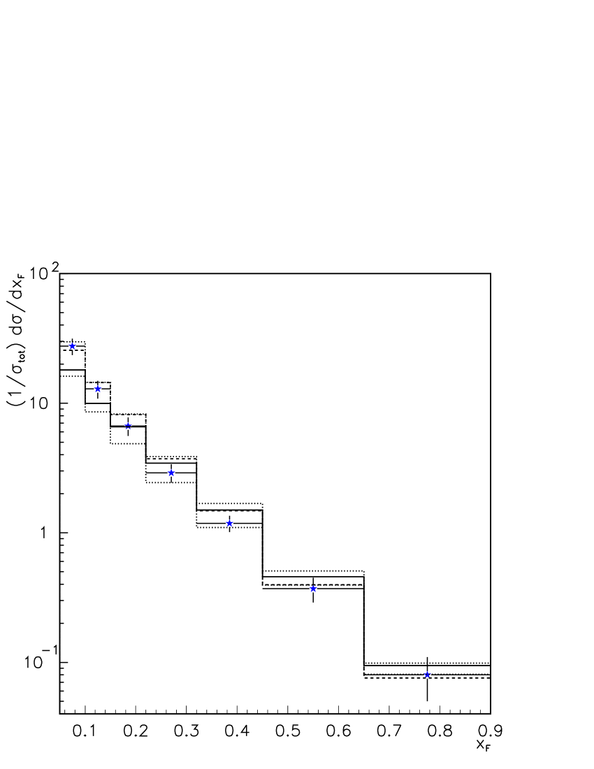
Figure 4.10: The dependence of the charged particle multiplicity on the Feynman variable $x_{F}$ in the hCM frame. The solid curve corresponds to the resummed multiplicity. The dashed, lower dotted and upper dotted curves correspond to the NLO multiplicity calculated for $\mu=Q,\,\,0.5Q$ and $2Q$, respectively.

4.3 Discussion and conclusions

The results in this Chapter demonstrate that multiple radiation of soft and collinear partons influence a large class of observables and can be described with the help of the CSS resummation formalism [32, 33]. Multiple parton radiation affects hadroproduction in the current region of deep-inelastic scattering, i.e., for large pseudorapidity of the final-state hadrons in the photon-proton c.m. frame.

Although the resummation formalism needs further development, in particular in the procedure for matching the resummed curve to the perturbative result in the transition region, it already improves the agreement between the theory and the data and provides interesting insights about qualitative features of SIDIS. The formalism describes well the behavior of the transverse energy flows measured at HERA [64, 65] in the region of large hCM pseudorapidity $\eta_{cm}\geq 3.0$. At smaller pseudorapidities the NLO rate falls below the existing data. Evidently, this is a signature of the importance of the NNLO corrections, which were not studied in this paper. The resummation formalism describes the pseudorapidity distributions of the transverse energy flow more accurately than the NLO calculation; this formalism also has good potential to improve the description of various distributions of particle multiplicity.

The presented analysis shows that the experimentally measured $q_{T}$ distributions for the energy flow broaden rapidly as $x\rightarrow 0$. This rapid broadening of the $q_{T}$ distributions can be realized if the nonperturbative Sudakov factor in the resummed energy flow increases as $1/x$. Similarly, the $q_{T}$ distribution for the charged particle multiplicity broadens rapidly when $z\rightarrow 0$, which is consistent with the nonperturbative Sudakov factor increasing as $z^{-1.4}$. The SIDIS nonperturbative Sudakov factors at small values of $x$ and $z$ are therefore qualitatively different from the known nonperturbative Sudakov factors for vector boson production and $e^{+}e^{-}$ hadroproduction, which do not depend on the longitudinal variables at all. The rapid growth of the nonperturbative Sudakov factor in SIDIS might indicate that the $ep$ collider HERA tests the resummation formalism in a new dynamical regime, which was not yet studied at colliders of other types. In particular, the CSS formula adopted here assumes the usual DGLAP physics for the evolution of initial and final state partons [47], in which the radiation of unobserved collinear partons is $k_{T}$-ordered. The broadening of the $q_{T}$ distributions may be a result of the increasing importance of $k_{T}$-unordered radiation in the limit $x\rightarrow 0$. The growth of the nonperturbative Sudakov factor $S^{NP}$ as $x$ decreases may be caused by the increase of the intrinsic transverse momentum of the probed partons due to such radiation.

There are several theoretical aspects of the resummation formalism that can be clarified when more experimental data are published. Perhaps the largest uncertainty in the predictions of the resummation formalism comes from the unknown nonperturbative contributions, which in the $b$-space formalism are included in the nonperturbative Sudakov factor $S^{NP}(b)$. I have presented simple parametrizations of $S^{NP}(b)$ for the transverse energy flow (cf. Eqs. (4.6,4.12)) and charged particle multiplicity (cf. Eq. (4.18)). These parametrizations were found by fitting the resummed energy flow and charged particle multiplicity to the data from Refs. [64, 65] and Ref. [60], respectively. Experimental measurements outside the range of those data will make it possible to further improve these parametrizations and, hence, the accuracy of the resummation formalism.

The most straightforward way to study $S^{NP}(b)$ is by measuring the variation of the $q_{T}$ spectra of physical quantities due to variations of one kinematical variable, with other variables fixed or varying only in a small range. For the energy flow, it would be beneficial to obtain more data at $x>10^{-2}$, where the predictions of the resummation formalism can be tested more reliably, without potential uncertainties due to the small-$x$ physics. Another interesting question is the dependence of the nonperturbative Sudakov factor on the virtuality $Q$ of the vector boson. This dependence can be tested by studying the $q_{T}$ spectra in a range of $Q$ with sufficient experimental resolution in the current fragmentation region. Finally, to study effects of multiple parton radiation on semi-inclusive production of individual hadrons, it will be interesting to see the $q_{T}$ spectra for particle production multiplicities with the additional constraint $z>0.05\sim 0.1$, i.e., in the kinematical region where the parametrizations of the fragmentation functions are known reasonably well.

Chapter 5 Azimuthal asymmetries of SIDIS observables

In a recent publication [61] the ZEUS Collaboration at DESY-HERA has presented data on asymmetries of charged particle ($h^{\pm}$) production in the process $e+p\stackrel{{\scriptstyle\gamma^{*}}}{{\longrightarrow}}e+h^{\pm}+X$, with respect to the angle $\varphi$ defined as the angle between the lepton scattering plane and the hadron production plane (of $h^{\pm}$ and the exchanged virtual photon). This angle is shown in Figure 3.3. The azimuthal asymmetries, $\langle\cos\varphi\rangle$ and $\langle\cos{2\varphi}\rangle$, as functions of the minimal transverse momentum $p_{c}$ of the observed charged hadron $h^{\pm}$ in the hadron-photon center-of-mass (hCM) frame, are defined as

$$\langle\cos n\varphi\rangle(p_{c})=\frac{\int d\Phi\int_{0}^{2\pi}d\varphi\cos n\varphi\frac{d\sigma}{dxdzdQ^{2}dp_{T}d\varphi}}{\int d\Phi\int_{0}^{2\pi}d\varphi\frac{d\sigma}{dxdzdQ^{2}dp_{T}d\varphi}},$$ (5.1)

with $n=1,2$. In terms of the momenta of the initial proton $p_{A}^{\mu}$, the final-state hadron $p_{B}^{\mu}$, and the exchanged photon $q^{\mu}$, the variables in (5.1) are $Q^{2}=-q_{\mu}q^{\mu}$, $x=Q^{2}/2(p_{A}\cdot q)$, and $z=(p_{A}\cdot p_{B})/(p_{A}\cdot q)$. $\int d\Phi$ denotes the integral over $x,z,Q^{2},p_{T}$ within the region defined by $0.01<x<0.1$, $180\mbox{\, GeV}^{2}<Q^{2}<7220\mbox{\, GeV}^{2}$, $0.2<z<1,\,\mbox{and\, }p_{T}>p_{c}$. Nonzero $\langle{\cos{2\varphi}}\rangle$ comes from interference of the helicity $+1$ and $-1$ amplitudes of the transverse photon polarization; and nonzero $\langle{\cos\varphi}\rangle$ comes from interference of transverse and longitudinal photon polarization.

More than 20 years ago it was proposed to test QCD by comparing measured azimuthal asymmetries to the perturbative predictions [92]. However, it was also realized that nonperturbative contributions and higher-twist effects may affect the comparison [72, 93, 94, 95]. For example, intrinsic $k_{T}$ might be used to parametrize the nonperturbative effects [93], and indeed ZEUS did apply this idea to their analysis of the data. The relative importance of the nonperturbative effects is expected to decrease as $p_{T}$ increases. Thus, the azimuthal asymmetries in semi-inclusive deep-inelastic scattering (SIDIS) events with large $p_{T}$ should be dominated by perturbative dynamics.

By comparing their data to the PQCD calculation at the leading order in $\alpha_{S}$ [96, 97, 98], the ZEUS Collaboration concluded that the magnitude of the measured asymmetry $\langle\cos\varphi\rangle$ exceeds the theoretical prediction for $p_{c}<1\mbox{\, GeV}$, and $\langle\cos 2\varphi\rangle$ is systematically above the theoretical prediction for $p_{c}>1.25$ GeV. ZEUS also estimated the possible nonperturbative contribution, by introducing a transverse momentum $k_{T}$ of the initial-state parton in the proton, and similarly of the final-state hadron due to nonperturbative fragmentation. It was found that this nonperturbative contribution is negligible for $\langle\cos 2{\varphi}\rangle$. For $\langle\cos{\varphi}\rangle$, the nonperturbative contribution can be sizable (up to 20%), but it is not large enough to account for the difference between the data and the ${\mathcal{O}}(\alpha_{S})$ calculation at low $p_{c}$. Hence, it was suggested that the discrepancy in $\langle\cos{\varphi}\rangle$ may be caused by large higher-order corrections.

From the comparison to the PQCD calculation at the leading order in $\alpha_{S}$ [96, 97], the ZEUS Collaboration concluded that the data on the azimuthal asymmetries at large values of $p_{c}$, although not well described by the QCD predictions, do provide clear evidence for a PQCD contribution to the azimuthal asymmetries. In this Chapter, the ZEUS data is discussed in a framework of QCD resummation formalism [17, 21, 32, 33, 35, 36, 37] that takes into account the effects of multiple soft parton emission. The discussion targets two objectives. First, it is shown that the analysis of $\langle\cos\varphi\rangle$ and $\langle\cos{2\varphi}\rangle$ based on fixed-order QCD is unsatisfactory because it ignores large logarithmic corrections due to soft parton emission. In addition, perturbative and nonperturbative contributions are mixed in the transverse momentum distributions, so that the presented data does not clarify the dynamical mechanism that generates the observed asymmetries. Second, I make two suggestions for improvement of the analysis of the ZEUS data. I show that perturbative and nonperturbative contributions can be separated more clearly in asymmetries depending on a variable $q_{T}$ related to the pseudorapidity of the final hadron in the hCM frame. I also suggest to measure the asymmetries of the transverse energy flow that are simpler and may be calculated reliably. I present numerical predictions for the asymmetries of transverse energy flow. These predictions are the most important result in this Chapter.

5.1 Large logarithmic corrections and resummation

The resummation formalism applied here was discussed in Chapter 3. It describes production of nearly massless hadrons in the current fragmentation region, where the production rate is the highest. In this region, transverse momentum distributions are affected by large logarithmic QCD corrections due to radiation of soft and collinear partons. The leading logarithmic contributions can be summed through all orders of PQCD [32, 33, 35, 36] by applying a method originally proposed for jet production in $e^{+}e^{-}$ annihilation [17] and vector boson production at hadron-hadron colliders [21].

According to Eq. (3.62), the spin-averaged cross section for SIDIS in a parity-conserving channel, e.g., $\gamma^{*}$ exchange, can be decomposed into a sum of independent contributions from four basis functions $A_{\rho}(\psi,\varphi)$ of the leptonic angular parameters $\psi,\varphi$ [34]:

$$\frac{d\sigma}{dxdzdQ^{2}dq_{T}^{2}d\varphi}=\sum_{\rho=1}^{4}{\,}^{\rho}{V}(x,z,Q^{2},q_{T}^{2})A_{\rho}(\psi,\varphi).$$

Here $\psi$ is the angle of a hyperbolic rotation (a boost) in Minkowski space; it is related to the conventional DIS variable $y$, by $y=Q^{2}/xS_{eA}=2/(1+\cosh\psi)$. The angular basis functions are $A_{1}=1+\cosh^{2}\psi$, $A_{2}=-2$, $A_{3}=-\cos\varphi\sinh 2\psi$, $A_{4}=\cos 2\varphi\sinh^{2}\psi$. Of the four structure functions ${\,}^{\rho}V$, only ${\,}^{1}V$ and ${\,}^{2}V$ contribute to the denominator of (5.1), i.e., the $\varphi$-integrated cross section. Of these two terms, ${\,}^{1}V$ is more singular, and it dominates the rate. According to the discussion in Chapter 3, the singular contributions in ${\,}^{1}V$ can be conveniently explored by introducing a scale $q_{T}$ related to the polar angle ($\theta_{B,cm}$) of the direction of the final hadron (B) in the hCM frame:

$$q_{T}=Q\sqrt{1/x-1}\,\exp{(-\eta_{cm})},$$ (5.2)

where $\eta_{cm}$ is the pseudorapidity of the charged hadron in the hCM frame. In the limit $q_{T}\rightarrow 0$, the structure function ${\,}^{1}V$ is dominated by large logarithmic terms; it has the form $q_{T}^{-2}\sum_{k=1}^{\infty}(\alpha_{S}/\pi)^{k}\sum_{m=0}^{2k-1}v^{(km)}\ln^{m}(q_{T}^{2}/Q^{2})$, where $v^{(km)}$ are some generalized functions. To obtain a stable theoretical prediction, these large terms must be resummed through all orders of PQCD. The other structure functions ${}^{2,3,4}V$ are finite at this order; they will be approximated by fixed-order ${\cal O}(\alpha_{S})$ expressions.

In Eq. (5.1), the numerator of $\langle\cos{\varphi}\rangle$ or $\langle\cos{2\varphi}\rangle$ depends only on the structure function ${\,}^{3}V$ or ${\,}^{4}V$, respectively. The measurement of $\langle\cos{\varphi}\rangle$ or $\langle\cos{2\varphi}\rangle$ must be combined with good knowledge of the $\varphi$-integrated cross section, i.e., the denominator of (5.1), to provide experimental information on the structure function ${\,}^{3}V$ or ${\,}^{4}V$. Thus it is crucial to check whether the theory can reproduce the $\varphi$-integrated cross section as a function of $p_{T}$ before comparing the prediction for (5.1) to the data. But Figure 4.9 shows that the ${\mathcal{O}}(\alpha_{S})$ fixed-order cross section is significantly lower than the data from [60] in the range of $p_{T}$ relevant to the ZEUS measurements. This difference signals the importance of higher-order corrections and undermines the validity of the ${\mathcal{O}}(\alpha_{S})$ result as a reliable approximation for the numerator of Eq. (5.1).

On the other hand, the resummation calculation with a proper choice of the nonperturbative function yields a much better agreement with the experimental data for the $p_{T}$-distribution from [60]. One might try to improve the theoretical description of the ZEUS data using resummation for the denominator of Eq. (5.1). However, the resummation calculation for $d\sigma/(dxdzdQ^{2}dq_{T}^{2}d\varphi)$ in the phase space region relevant to the ZEUS data is currently not possible, largely because of the uncertainty in the parametrization of the nonperturbative contributions in this region. The impact parameter ($b$-space) resummation formalism [32, 33] includes a nonperturbative Sudakov factor , which contains the effects of the intrinsic transverse momentum of the initial-state parton and the nonperturbative fragmentation contributions to the transverse momentum of the final-state hadron (cf. Eq. (3.112)). Without first determining this nonperturbative factor, e.g., from other measurements, it is not possible to make a trustworthy theoretical prediction for the denominator of Eq. (5.1) and, hence, these azimuthal asymmetries.

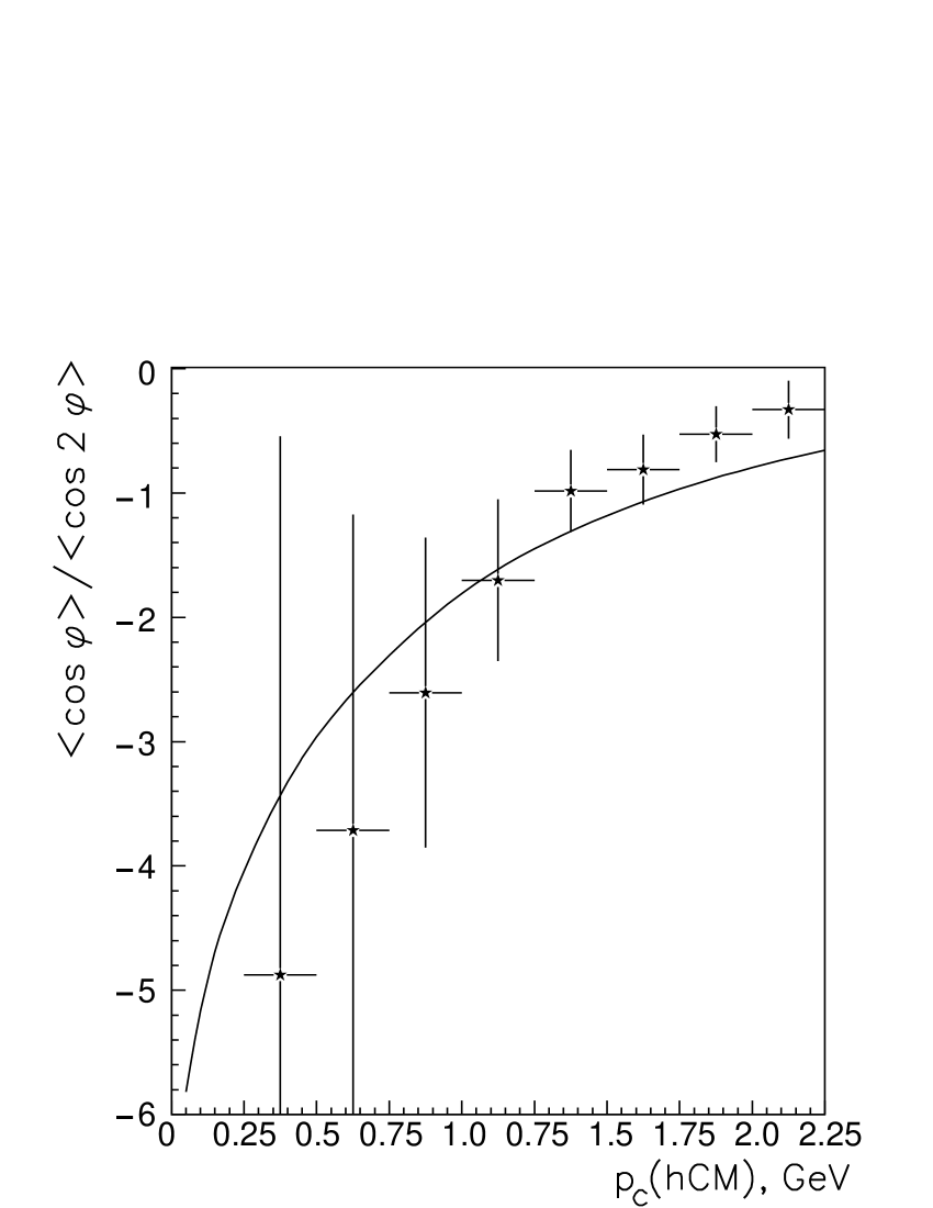
Figure 5.1: Comparison of the ${\mathcal{O}}(\alpha_{S})$ prediction for the ratio $\langle\cos\varphi\rangle/\langle\cos{2\varphi}\rangle$ with the ratio of experimentally measured values of $\langle\cos\varphi\rangle$ and $\langle\cos{2\varphi}\rangle$ from [61]. The error bars are calculated by adding the statistical errors of $\langle\cos\varphi\rangle$ and $\langle\cos{2\varphi}\rangle$ in quadrature. Systematic errors are not included. The theoretical curve is calculated for $\langle x\rangle=0.022$, $\langle Q^{2}\rangle=750\mbox{\, GeV}^{2}$, using the CTEQ5M1 parton distribution functions [90] and fragmentation functions by S. Kretzer from [88].

The azimuthal asymmetries measured by ZEUS may also be sensitive to uncertainties in the fragmentation to $h^{\pm}$ in the final state. Indeed, the cross section in Eq. (5.1) includes convolutions of hard scattering cross sections with fragmentation functions (FFs), integrated over the range $0.2<z<1$. Although the knowledge of FFs is steadily improving [87, 88, 89], there is still some uncertainty about their $z$-dependence and flavor structure for the range of $Q$ relevant to the ZEUS measurement. Therefore the most reliable tests of the theory would use observables that are not sensitive to the final-state fragmentation. The asymmetries $\langle\cos n\varphi\rangle$ would be insensitive to FFs if the dependence on the partonic variable $\widehat{z}$ were similar in the hard parts of the numerator and denominator of Eq. (5.1), so that the dependence on the FFs would approximately cancel. It is shown in Appendix A that the partonic structure function ${\,}^{1}\widehat{V}$, which dominates the denominator of (5.1), contains terms proportional to $1/\widehat{z}^{2}$ that increase rapidly as $\widehat{z}$ decreases. However, the most singular terms in the partonic structure functions ${\,}^{3,4}\widehat{V}$ are proportional to $1/\widehat{z}$. Therefore, the dependence on the FFs does not cancel in the azimuthal asymmetries.

A curious fact appears to support the suggestion that the theoretical predictions for $\langle\cos n\varphi\rangle$ depend significantly on the fragmentation functions. While each of the measured asymmetries, $\langle\cos\varphi\rangle$ and $\langle\cos 2\varphi\rangle$, deviates from the ${\mathcal{O}}(\alpha_{S})$ prediction, the data actually agree well with the ${\mathcal{O}}(\alpha_{S})$ prediction for the ratio $\langle\cos\varphi\rangle/\langle\cos 2\varphi\rangle$, as shown in Fig. 5.1. The error bars are the statistical errors on $\langle{\cos\varphi}\rangle$ and $\langle\cos{2\varphi}\rangle$ combined in quadrature; this may overestimate the experimental uncertainty if the two errors are correlated. Since this ratio depends only on the numerators in Eq. (5.1), which are less singular with respect to $\widehat{z}$ than the denominator, the dependence on the fragmentation functions may be nearly canceled in the ratio. The good agreement between the ${\mathcal{O}}(\alpha_{S})$ prediction and the experimental data for this ratio supports our conjecture that the fragmentation dynamics has a significant impact on the individual asymmetries defined in Eq. (5.1).

The final remark about the azimuthal asymmetries in Eq. (5.1) is that the $p_{T}$ (or $p_{c}$) distributions are not the best observables to separate the perturbative and nonperturbative effects. The region where multiple parton radiation effects are important is specified by the condition $q_{T}^{2}/Q^{2}\ll 1$. But the $p_{T}$ distributions are smeared with respect to the $q_{T}$ distributions by an additional factor of $z$, because $p_{T}=z\,\,q_{T}$. Thus the whole observable range of $p_{T}$ is sensitive to the resummation effects in the region of $q_{T}$ of the order of several GeV. A better way to compare the data to the PQCD prediction is to express the azimuthal asymmetries as a function of $q_{T}$, not $p_{T}$. Then the comparison should be made in the region where the multiple parton radiation is unimportant, i.e., for $q_{T}/Q\gtrsim 1$.

5.2 Asymmetry of energy flow

Next, I describe an alternative test of PQCD, which is less sensitive to the above theoretical uncertainties: measurement of the azimuthal asymmetries of the transverse energy flow. In the hCM frame, the transverse energy flow can be written as [86, 34, 33, 35, 36]

$$\frac{dE_{T}}{dxdQ^{2}dq_{T}^{2}d\varphi}=\sum_{\rho=1}^{4}{\,}^{\rho}V_{E_{T}}(x,Q^{2},q_{T}^{2})A_{\rho}(\psi,\varphi).$$ (5.3)

Unlike the charged particle multiplicity, the energy flow does not depend on the final-state fragmentation. According to the results in Chapter 4, a resummation calculation can provide a good description for the experimental data on the $\varphi$-integrated $E_{T}$-flow. A new class of azimuthal asymmetries may be defined as

$$\langle E_{T}\cos n\varphi\rangle(q_{T})=\frac{\int d\Phi\int_{0}^{2\pi}\cos n\varphi\frac{dE_{T}}{dxdQ^{2}dq_{T}^{2}d\varphi}d\varphi}{\int d\Phi\int_{0}^{2\pi}\frac{dE_{T}}{dxdQ^{2}dq_{T}^{2}d\varphi}d\varphi}.$$ (5.4)

The structure functions ${\,}^{\rho}V_{E_{T}}$ for the $E_{T}$-flow can be derived from the structure functions ${\,}^{\rho}V$ for the SIDIS cross section using Eq. (3.122). Similar to the case of the particle multiplicities, the asymmetries $\langle E_{T}\cos\varphi\rangle$ and $\langle E_{T}\cos 2\varphi\rangle$ receive contributions from ${\,}^{3}V_{E_{T}}$ and ${\,}^{4}V_{E_{T}}$, respectively. But, unlike the previous case, the denominator in Eq. (5.4) is approximated well by the resummed $E_{T}$-flow. Thus these asymmetries can be calculated with greater confidence.

Figure 5.2 shows the prediction for the azimuthal asymmetries $\langle E_{T}\cos\varphi\rangle$ and $\langle E_{T}\cos 2\varphi\rangle$ as functions of $q_{T}$ for (a) $x=0.0047$, $Q^{2}=33.2\mbox{\, GeV}^{2}$ in the left plots and (b) $x=0.026$, $Q^{2}=617\mbox{\, GeV}^{2}$ in the right plots. The asymmetries are shown in $q_{T}$-bins that are obtained from the experimental pseudorapidity bins for the $\varphi$-integrated $E_{T}$-flow data from Ref. [65]. The upper $x$-axis shows values of the hCM pseudorapidity $\eta_{cm}$ that correspond to the values of $q_{T}$ on the lower $x$-axis. For each of the distributions in Fig. 5.2, the structure functions ${\,}^{3}V_{E_{T}}$ and ${\,}^{4}V_{E_{T}}$ were calculated at leading order in QCD, i.e., ${\mathcal{O}}(\alpha_{S})$. The solid and dashed curves, which correspond to the resummed and ${\mathcal{O}}(\alpha_{S})$ results respectively, differ because the structure function ${\,}^{1}V_{E_{T}}$ in the denominator of (5.4) differs for the two calculations. The resummed $\varphi$-integrated $E_{T}$-flow is closer to the data than the fixed-order result, so that the predictions made by PQCD for the subleading structure functions ${\,}^{3}V_{E_{T}}$ and ${\,}^{4}V_{E_{T}}$ will be confirmed if the experimental azimuthal asymmetries agree with the resummed distributions.

The discussion in Section 4.1 shows that in the region $q_{T}\sim Q$ the resummed $\varphi$-integrated $E_{T}$-flow is larger than the ${\mathcal{O}}(\alpha_{S})$ prediction. This explains why the asymmetries for $q_{T}\sim Q$ are smaller for the resummed denominator than for the ${\mathcal{O}}(\alpha_{S})$ denominator. In the region $q_{T}/Q\ll 1$, the asymmetries are determined by the asymptotic behavior of the fixed-order and resummed partonic structure functions ${\,}^{\rho}\widehat{V}_{E_{T}}$. As $q_{T}\rightarrow 0$, the ${\mathcal{O}}(\alpha_{S})$ structure functions $({\,}^{1}\widehat{V}_{E_{T}})_{{\mathcal{O}}(\alpha_{S})}$, ${\,}^{3}\widehat{V}_{E_{T}}$, and ${\,}^{4}\widehat{V}_{E_{T}}$ behave as $1/q_{T}^{2}$, $1/q_{T}$ and $1$, respectively. Thus, asymptotically, the ratios ${\,}^{3,4}\widehat{V}_{E_{T}}/({\,}^{1}\widehat{V}_{E_{T}})_{{\mathcal{O}}(\alpha_{S})}$ go to zero, although the $q_{T}$ distribution for the asymmetry $\langle E_{T}\cos\varphi\rangle$ is quite large and negative for small, but non-vanishing $q_{T}$ (cf. Fig. 5.2). Resummation of ${\,}^{1}\widehat{V}_{E_{T}}$ changes the $q_{T}$-dependence of the denominator, which becomes nonsingular in the limit $q_{T}\rightarrow 0$. Consequently, the asymmetry $\langle E_{T}\cos\varphi\rangle$ with the resummed denominator asymptotically grows as $1/q_{T}$ (i.e., in accordance with the asymptotic behavior of ${\,}^{3}\widehat{V}_{E_{T}}$). Hence neither the fixed-order nor the resummed calculation for $\langle E_{T}\cos\varphi\rangle$ is reliable in the low-$q_{T}$ region, so that higher-order or additional nonperturbative contributions must be important at $q_{T}\rightarrow 0$. The asymptotic limit for the resummed $\langle E_{T}\cos 2\varphi\rangle$ remains finite, with the magnitude shown in Fig. 5.2. Since the magnitude of $\langle E_{T}\cos 2\varphi\rangle$ is predicted not to exceed a few percent, an experimental observation of a large asymmetry $\langle E_{T}\cos 2\varphi\rangle$ at small $q_{T}$ would signal the presence of some new hadronic dynamics, e.g., contributions from $T$-odd structure functions discussed in [95].

Figure 5.2 shows that the predicted asymmetry $\langle E_{T}\cos\varphi\rangle(q_{T})$ at $q_{T}/Q=1$ is about 1–2% for the resummed denominator, while it is about 2–4% for the ${\mathcal{O}}(\alpha_{S})$ denominator. The asymmetry $\langle E_{T}\cos 2\varphi\rangle(q_{T})$ at $q_{T}/Q=1$ is about 1.5-2% or 3.5-5%, respectively. Both asymmetries are positive for $q_{T}\sim Q$. According to Fig. 5.2a, the size of the experimental $q_{T}$ bins (converted from the $\eta$ bins in [65]) for low or intermediate values of $Q^{2}$ is small enough to reveal the low-$q_{T}$ behavior of ${\,}^{3,4}V_{E_{T}}$ with acceptable accuracy. However, for the high-$Q^{2}$ events in Fig. 5.2b, the experimental resolution in $q_{T}$ may be insufficient for detailed studies in the low-$q_{T}$ region. Nonetheless, it will still be interesting to compare the experimental data to the predictions of PQCD in the region $q_{T}/Q\approx 1$, and to learn about the angular asymmetries at large values of $Q^{2}$ and $x$.

To conclude, the azimuthal asymmetry of the energy flow should be measured as a function of the scale $q_{T}$. These measurements would test the predictions of the PQCD theory more reliably than the measurements of the asymmetries of the charged particle multiplicity.

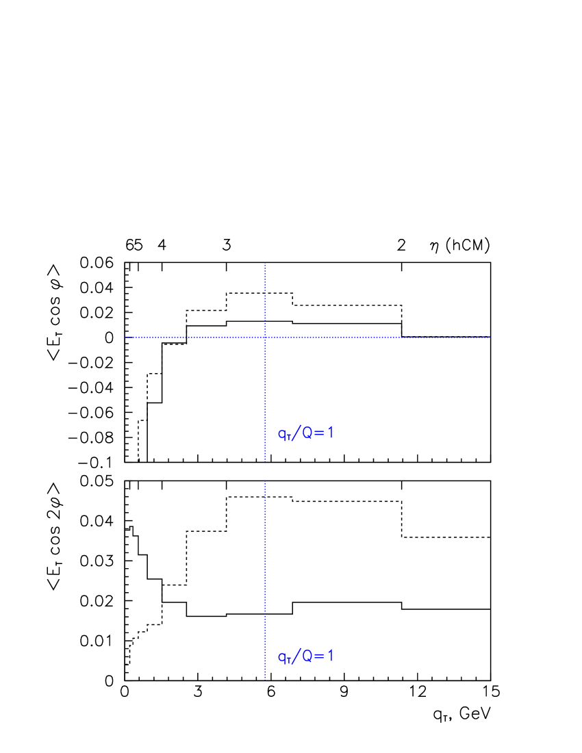
a)

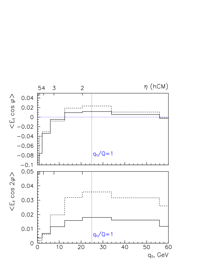
b)

Figure 5.2: Energy flow asymmetries $\langle E_{T}\cos\varphi\rangle(q_{T})$ and $\langle E_{T}\cos{2\varphi}\rangle(q_{T})$ for (a) $x=0.0047$, $Q^{2}=33.2\mbox{\, GeV}^{2}$ and (b) $x=0.026$, $Q^{2}=617\mbox{\, GeV}^{2}$. The Figure shows predictions from the resummed (solid) and the ${\mathcal{O}}(\alpha_{S})$ (dashed) calculations.

Appendix A The perturbative cross-section, finite piece and $z$-flow distribution

In this Appendix, I collect the formulas for the NLO parton level cross-sections $d\widehat{\sigma}_{ba}/(d\widehat{x}d\widehat{z}dQ^{2}dq_{T}^{2}d\varphi)$, which were originally obtained in [98].

According to Eqs. (3.60,3.63), the hadron level cross-section $d\sigma_{BA}/(dxdzdQ^{2}dq_{T}^{2}d\varphi)$ is related to the parton-level structure functions ${\,}^{\rho}{\widehat{V}}_{ba}$ as

$$\frac{d\sigma_{BA}}{dxdzdQ^{2}dq_{T}^{2}d\varphi}=\sum_{\rho=1}^{4}A_{\rho}(\psi,\varphi)\times$$ (A.1)

$$\times \sum_{a,b}\int_{z}^{1}\frac{d\xi_{b}}{\xi_{b}}D_{B/b}(\xi_{b},\mu)\int_{x}^{1}\frac{d\xi_{a}}{\xi_{a}}F_{a/A}(\xi_{a},\mu){\,}^{\rho}{\widehat{V}}_{ba}(\widehat{x},\widehat{z},Q^{2},q_{T}^{2},\mu).$$

At non-zero $q_{T}$, the parton cross-section receives the contribution from the real emission diagrams (Fig. 3.6e-f), so that ${\,}^{\rho}{\widehat{V}}_{ba}$ can be expressed as

$${\,}^{\rho}{\widehat{V}}_{ba}=\frac{\sigma_{0}F_{l}}{4\pi S_{eA}}\frac{\alpha_{S}}{\pi}\delta\Biggl{[}\frac{q_{T}^{2}}{Q^{2}}-\Bigl{(}\frac{1}{\widehat{x}}-1\Bigr{)}\Bigl{(}\frac{1}{\widehat{z}}-1\Bigr{)}\Biggr{]}{\,}^{\rho}f_{ba}(\widehat{x},\widehat{z},Q^{2},q_{T}^{2}),$$ (A.2)

with the same notations as in Chapter 3. In this Equation, the $q\bar{q}$ structure functions are

$${}^{\rho}f_{jk}(\widehat{x},\widehat{z},Q^{2},q_{T}^{2})\equiv 2C_{F}\widehat{x}\widehat{z}e_{j}^{2}\delta_{jk}\,\,{}^{\rho}\bar{f}_{jk},$$ (A.3)

where

$${}^{1}\bar{f}_{jk} = \frac{1}{Q^{2}q_{T}^{2}}\biggl{(}\frac{Q^{4}}{\widehat{x}^{2}\widehat{z}^{2}}+(Q^{2}-q_{T}^{2})^{2}\biggr{)}+6;$$

$${}^{2}\bar{f}_{jk} = 2\,\,({}^{4}\bar{f}_{jk})=4;$$

$${}^{3}\bar{f}_{jk} = \frac{2}{Qq_{T}}\left(Q^{2}+q_{T}^{2}\right).$$ (A.4)

The $\stackrel{{\scriptstyle(-)}}{{q}}g$ structure functions are

$${\,}^{\rho}f_{jg}(\widehat{x},\widehat{z},Q^{2},q_{T}^{2})\equiv\widehat{x}(1-\widehat{x})e_{j}^{2}\,\,{\,}^{\rho}\bar{f}_{jg},$$ (A.5)

where

$${\,}^{1}\bar{f}_{jg} = \frac{Q^{2}}{q_{T}^{2}}\biggl{(}\frac{1}{\widehat{x}^{2}\widehat{z}^{2}}-\frac{2}{\widehat{x}\widehat{z}}+2\biggr{)}+10-\frac{2}{\widehat{x}}-\frac{2}{\widehat{z}};$$

$${\,}^{2}\bar{f}_{jg} = 2\,\,({\,}^{4}\bar{f}_{jg})=8;$$

$${\,}^{3}\bar{f}_{jg} = \frac{2}{Qq_{T}}\left(2(Q^{2}+q_{T}^{2})-\frac{Q^{2}}{\widehat{x}\widehat{z}}\right).$$ (A.6)

Finally, the $g\stackrel{{\scriptstyle(-)}}{{q}}$ structure functions are

$${\,}^{\rho}f_{gj}(\widehat{x},\widehat{z},Q^{2},q_{T}^{2})\equiv 2C_{F}\widehat{x}(1-\widehat{z})e_{j}^{2}\,\,{\,}^{\rho}\bar{f}_{gj},$$ (A.7)

where

$${\,}^{1}\bar{f}_{gj} = \frac{1}{Q^{2}\tilde{q}_{T}^{2}}\biggl{(}\frac{Q^{4}}{\widehat{x}^{2}(1-\widehat{z})^{2}}+(Q^{2}-\tilde{q}_{T}^{2})^{2}\biggr{)}+6;$$

$${\,}^{2}\bar{f}_{gj} = 2\,\,({\,}^{4}\bar{f}_{gj})=4;$$

$${\,}^{3}\bar{f}_{gj} = \frac{2}{Q\tilde{q}_{T}}\left(Q^{2}+\tilde{q}_{T}^{2}\right).$$ (A.8)

In (A.8),

$$\tilde{q}_{T}\equiv\frac{\widehat{z}q_{T}}{1-\widehat{z}}.$$ (A.9)

The indices $j$ and $k$ correspond to a quark (antiquark) of a type $j$ or $k$, the index $g$ corresponds to a gluon.

The finite part $Y_{BA}$ of the ${\cal O}(\alpha_{S})$ cross section (A.1) is

$$Y_{BA}=\frac{\sigma_{0}F_{l}}{4\pi S_{eA}}\frac{\alpha_{S}}{\pi}\sum_{\rho=1}^{4}A_{\rho}(\psi,\varphi)\sum_{a,b}\int_{z}^{1}\frac{d\xi_{b}}{\xi_{b}}D_{B/b}(\xi_{b},\mu)\int_{x}^{1}\frac{d\xi_{a}}{\xi_{a}}F_{a/A}(\xi_{a},\mu)\times$$ (A.10)

$$\times {\,}^{\rho}{R}_{ba}(\widehat{x},\widehat{z},Q^{2},q_{T}^{2},\mu).$$

For $\rho=1$, the functions ${\,}^{\rho}{R_{ba}}$ are

$${\,}^{1}R_{jk}(\widehat{x},\widehat{z},Q^{2},q_{T}^{2}) = \delta\left[\frac{q_{T}^{2}}{Q^{2}}-\left(\frac{1}{\widehat{x}}-1\right)\left(\frac{1}{\widehat{z}}-1\right)\right]{}^{1}f_{jk}(\widehat{x},\widehat{z},Q^{2},q_{T}^{2})$$ (A.11)

$$- \frac{1}{q_{T}^{2}}\delta_{jk}e_{j}^{2}\Biggl{\{}\delta(1-\widehat{z})P^{(1)}_{qq}(\widehat{x})+P^{(1)}_{qq}(\widehat{z})\delta(1-\widehat{x})$$

$$+ 2C_{F}\delta(1-\widehat{z})\delta(1-\widehat{x})\left(\log\frac{Q^{2}}{q_{T}^{2}}-\frac{3}{2}\right)\Biggr{\}};$$

$${\,}^{1}R_{jg}(\widehat{x},\widehat{z},Q^{2},q_{T}^{2}) = \delta\left[\frac{q_{T}^{2}}{Q^{2}}-\left(\frac{1}{\widehat{x}}-1\right)\left(\frac{1}{\widehat{z}}-1\right)\right]{}^{1}f_{jg}(\widehat{x},\widehat{z},Q^{2},q_{T}^{2})$$ (A.12)

$$- \frac{1}{q_{T}^{2}}e_{j}^{2}\delta(1-\widehat{z})P_{qg}^{(1)}(\widehat{x});$$

$${\,}^{1}R_{gj}(\widehat{x},\widehat{z},Q^{2},q_{T}^{2}) = \delta\left[\frac{q_{T}^{2}}{Q^{2}}-\left(\frac{1}{\widehat{x}}-1\right)\left(\frac{1}{\widehat{z}}-1\right)\right]{}^{1}f_{gj}(\widehat{x},\widehat{z},Q^{2},q_{T}^{2})$$ (A.13)

$$- \frac{1}{q_{T}^{2}}e_{j}^{2}P_{gq}^{(1)}(\widehat{z})\delta(1-\widehat{x}).$$

For $\rho=2,3,4$,

$${\,}^{\rho}R_{ba}(\widehat{x},\widehat{z},Q^{2},q_{T}^{2})=\delta\left[\frac{q_{T}^{2}}{Q^{2}}-\left(\frac{1}{\widehat{x}}-1\right)\left(\frac{1}{\widehat{z}}-1\right)\right]{}^{\rho}f_{ba}(\widehat{x},\widehat{z},Q^{2},q_{T}^{2}).$$ (A.14)

From (3.60), it is possible to derive the perturbative $z$-flow distribution,

$$\frac{d\Sigma_{z}}{dxdQ^{2}dq_{T}^{2}d\varphi}\equiv\sum_{B}\int_{z_{min}}^{1}zdz\frac{d\sigma_{BA}}{dxdzdQ^{2}dq_{T}^{2}d\varphi}=$$

$$\frac{\sigma_{0}F_{l}}{4\pi S_{eA}}\frac{\alpha_{S}}{\pi}\sum_{a,b}\sum_{j}e^{2}_{j}\int_{x}^{1}\frac{d\xi_{a}}{\xi_{a}-x}F_{a/A}(\xi_{a})\widehat{z}^{3}\widehat{x}\sum_{\rho=1}^{4}{\,}^{\rho}f_{ba}(\widehat{x},\widehat{z},Q^{2},q_{T}^{2})A_{\rho}(\psi,\varphi).$$ (A.15)

It depends on the same functions ${\,}^{\rho}f_{ba}(\widehat{x},\widehat{z},Q^{2},q_{T}^{2})$, with the parton variable $\widehat{z}$ determined by the $\delta$-function in (A.2),

$$\widehat{z}=\frac{1-\widehat{x}}{\left(q_{T}^{2}/Q^{2}-1\right)\widehat{x}+1}.$$ (A.16)

Appendix B ${\cal O}(\alpha_{S})$ part of the resummed cross section

In this Appendix, I demonstrate that the ${\cal O}(\alpha_{S})$ part of the $\widetilde{W}$-term in the resummed cross section (3.88) coincides with the small-$q_{T}$ approximation of the factorized ${\cal O}(\alpha_{S})$ fixed-order cross section. Correspondingly the complete ${\cal O}(\alpha_{S})$ part does not depend on the scales $C_{1}/b$ and $C_{2}Q$ separating collinear-soft and collinear contributions to the resummed cross section.

At $q_{T}\ll Q$, the resummed cross section (3.88) is dominated by the $\widetilde{W}$-term:

$$\left.\frac{d\sigma_{BA}}{dxdzdQ^{2}dq_{T}^{2}d\varphi}\right|_{resum} \approx \frac{\sigma_{0}F_{l}}{S_{eA}}\frac{A_{1}(\psi,\varphi)}{2}\int\frac{d^{2}b}{(2\pi)^{2}}e^{i\vec{q}_{T}\cdot\vec{b}}\widetilde{W}_{BA}(b)=$$ (B.1)

$$= \frac{\sigma_{0}F_{l}}{S_{eA}}\frac{A_{1}(\psi,\varphi)}{2Q^{2}}\int\frac{d^{2}\beta}{(2\pi)^{2}}e^{i\frac{\vec{q}_{T}\cdot\vec{\beta}}{Q}}\widetilde{W}_{BA}(\frac{\beta}{Q}),$$

where

$$\vec{\beta}\equiv Q\vec{b}.$$ (B.2)

According to Eq. (3.92), at $b\rightarrow 0$

$$\widetilde{W}_{BA}(b,Q,x,z)=\sum_{j}e_{j}^{2}(D_{B/b}\otimes{\cal C}^{out}_{bj})(z,b)({\cal C}_{ja}^{in}\otimes F_{a/A})(x,b)e^{-S^{P}(b,Q)}.$$ (B.3)

The perturbative Sudakov factor $S^{P}$and the ${\cal C}-$functions in $\widetilde{W}_{BA}(b,Q,x,z)$ can be expanded up to ${\cal O}(\alpha_{S})$ using Eqs. (3.93,3.101-3.109)

$$S^{P}(b,Q)\equiv\int_{C_{1}^{2}/b^{2}}^{C_{2}^{2}Q^{2}}\frac{d\overline{\mu}^{2}}{\overline{\mu}^{2}}\left({\cal A}(\alpha_{S}(\overline{\mu}),C_{1})\ln\frac{C_{2}^{2}Q^{2}}{\overline{\mu}^{2}}+{\cal B}(\alpha_{S}(\overline{\mu}),C_{1},C_{2})\right)\approx$$

$$\approx\frac{\alpha_{S}}{\pi}\left(\frac{{\cal A}_{1}}{2}\ln^{2}\frac{C^{2}_{2}Q^{2}b^{2}}{C^{2}_{1}}+{\cal B}_{1}(\alpha_{S}(\overline{\mu}),C_{1},C_{2})\ln\frac{C^{2}_{2}Q^{2}b^{2}}{C^{2}_{1}}\right)+{\cal O}(\alpha_{S}^{2})$$

$$\approx\frac{\alpha_{S}}{\pi}C_{F}\left(\frac{1}{2}\ln^{2}\frac{C^{2}_{2}Q^{2}b^{2}}{C^{2}_{1}}-\frac{3}{2}\ln\frac{C^{2}_{2}Q^{2}b^{2}}{C^{2}_{1}}-2\ln\frac{C_{2}b_{0}}{C_{1}}\ln\frac{C^{2}_{2}Q^{2}b^{2}}{C^{2}_{1}}\right);$$ (B.4)

$$({\cal C}_{ja}^{in}\otimes F_{a/A})(x,b,\mu)=F_{a/A}(x,\mu)\left(1+\frac{\alpha_{S}}{\pi}C_{F}\left(-\ln^{2}\frac{C_{1}}{C_{2}b_{0}}+\frac{3}{2}\ln\frac{C_{1}}{C_{2}b_{0}}\right)\right)$$

$$+\frac{\alpha_{S}}{\pi}\left((c^{(1)in}_{ja}\otimes F_{a/A})(x,\mu)-(\ln\frac{\mu b}{b_{0}}P_{ja}^{(1)}\otimes F_{a/A})(x,\mu)\right);$$ (B.5)

$$(D_{B/b}\otimes{\cal C}^{out}_{bj})(z,b,\mu)=D_{B/b}(z,\mu)\left(1+\frac{\alpha_{S}}{\pi}C_{F}\left(-\ln^{2}\frac{C_{1}}{C_{2}b_{0}}+\frac{3}{2}\ln\frac{C_{1}}{C_{2}b_{0}}\right)\right)$$

$$+\frac{\alpha_{S}}{\pi}\left((D_{B/b}\otimes c^{(1)out}_{bj})(z,\mu)-(D_{B/b}\otimes\ln\frac{\mu b}{\widehat{z}b_{0}}P_{bj}^{(1)})(z,\mu)\right),$$ (B.6)

where the functions $c_{ba}^{(1)in}$, $c^{(1)out}_{ba}$ are defined in Eqs. (3.82-3.84). In these equations the running of $\alpha_{S}$, which is an effect of ${\cal O}(\alpha_{S}^{2})$, is neglected. Inserting the ${\cal O}(\alpha_{S})$ representations (B.4-B.6) in Eq. (B.3), we obtain the ${\cal O}(\alpha_{S})$ expression for $\widetilde{W}_{BA}(b,Q,x,z):$

$$\left.\widetilde{W}_{BA}(\frac{\beta}{Q},Q,x,z)\right|_{{\cal O}(\alpha_{S})}=\sum_{j}e_{j}^{2}\times$$

$$\Biggl{\{}D_{B/j}(z,\mu)F_{j/A}(x,\mu)\left[1-\frac{\alpha_{S}}{\pi}C_{F}\left(\frac{1}{2}\ln^{2}\frac{\beta^{2}}{b_{0}^{2}}-\frac{3}{2}\ln\frac{\beta^{2}}{b_{0}^{2}}\right)\right]$$

$$+\frac{\alpha_{S}}{\pi}\Biggl{[}\left((D_{B/b}\otimes c^{(1)out}_{bj})(z,\mu)-(D_{B/b}\otimes\ln\left[\frac{\mu}{\widehat{z}Q}\frac{\beta}{b_{0}}\right]P_{bj}^{(1)})(z,\mu)\right)F_{j/A}(x,\mu)$$

$$+D_{B/j}(z,\mu)\left((c^{(1)in}_{ja}\otimes F_{a/A})(x,\mu)-(\ln\left[\frac{\mu}{Q}\frac{\beta}{b_{0}}\right]P_{ja}^{(1)}\otimes F_{a/A})(x,\mu)\right)\Biggr{]}\Biggr{\}}.$$

(B.7)

This expression does not depend on the constants $C_{1},C_{2}$, so that the only factorization scale in Eq. (B.7) is $\mu$. The Fourier-Bessel transform of $\widetilde{W}_{BA}(b,Q,x,z)$ to the $q_{T}$-space can be realized by using relationships

$$\int\frac{d^{2}b}{(2\pi)^{2}}e^{-i\vec{q}_{T}\cdot\vec{b}} = \delta(\vec{q}_{T});$$ (B.8)

$$\int\frac{d^{2}b}{(2\pi)^{2}}e^{-i\vec{q}_{T}\cdot\vec{b}}\ln\frac{b^{2}}{b_{0}^{2}} = -\frac{1}{\pi}\left[\frac{1}{q^{2}_{T}}\right]_{+};$$ (B.9)

$$\int\frac{d^{2}b}{(2\pi)^{2}}e^{-i\vec{q}_{T}\cdot\vec{b}}\ln^{2}\frac{b^{2}}{b_{0}^{2}} = \frac{2}{\pi}\left[\frac{\ln q_{T}^{2}}{q^{2}_{T}}\right]_{+},$$ (B.10)

where the “+”-prescription is defined as

$$\int d^{2}q_{T}\left[f(q_{T})\right]_{+}g(\vec{q}_{T})=\int_{0}^{2\pi}d\varphi\int^{+\infty}_{0}q_{T}dq_{T}f(q_{T})\left(g(\vec{q}_{T})-g(\vec{0})\right).$$ (B.11)

Hence the small-$q_{T}$ approximation for the ${\cal O}(\alpha_{S})$cross-section is

$$\left.\frac{d\sigma_{BA}}{dxdzdQ^{2}dq_{T}^{2}d\varphi}\right|_{{\cal O}(\alpha_{S}),q_{T}\rightarrow 0} = \frac{\sigma_{0}F_{l}}{S_{eA}}\frac{A_{1}(\psi,\varphi)}{2}\sum_{j}e_{j}^{2}\times$$ (B.12)

$$\times \left(\delta(\vec{q}_{T})F_{\delta}(x,z,Q,\mu)+F_{+}(x,z,Q,q_{T},\mu)\right),$$

where

$$F_{\delta}(x,z,Q,\mu)=D_{B/j}(z,\mu)F_{j/A}(x,\mu)+$$ (B.13)

$$\frac{\alpha_{S}}{\pi}\Biggl{\{}\left((D_{B/b}\otimes c^{(1)out}_{bj})(z,\mu)-(D_{B/b}\otimes\ln\left[\frac{\mu}{\widehat{z}Q}\right]P_{bj}^{(1)})(z,\mu)\right)F_{j/A}(x,\mu)$$

$$+ D_{B/j}(z,\mu)\left((c^{(1)in}_{ja}\otimes F_{a/A})(x,\mu)-(\ln\left[\frac{\mu}{Q}\right]P_{ja}^{(1)}\otimes F_{a/A})(x,\mu)\right)\Biggr{\}};$$

$$F_{+}(x,z,Q,q_{T},\mu)=\frac{1}{2\pi Q^{2}}\frac{\alpha_{S}}{\pi}\times$$ (B.14)

$$\Biggl{\{}2C_{F}D_{B/j}(z,\mu)F_{j/A}(x,\mu)\left(\left[\frac{Q^{2}}{q_{T}^{2}}\ln\frac{Q^{2}}{q_{T}^{2}}\right]_{+}-\frac{3}{2}\left[\frac{Q^{2}}{q^{2}_{T}}\right]_{+}\right)+\left[\frac{Q^{2}}{q_{T}^{2}}\right]_{+}\times$$

$$\times \left((D_{B/b}\otimes P_{bj}^{(1)})(z,\mu)F_{j/A}(x,\mu)+D_{B/j}(z.\mu)(P_{ja}^{(1)}\otimes F_{a/A})(x,\mu)\right)\Biggr{\}}.$$

The function $F_{\delta}(x,z,\mu)$ contributes at $q_{T}=0$; it receives contributions from the leading order scattering, evolution of the PDFs between the scales $\mu$ and $Q$, evolution of the FFs between the scales $\mu$ and $\widehat{z}Q$, and ${\cal O}(\alpha_{S})$ coefficient functions $c^{(1)in},$ $c^{(1)out}$. The function $F_{+}(x,z,Q,q_{T},\mu)$ is just a regularized asymptotic part (3.74) of the ${\cal O}(\alpha_{S})$ fixed-order structure function ${\,}^{1}V_{BA}$ (cf. Eq. (3.74)).

The ${\cal O}(\alpha_{S})$ cross section (B.12) can be integrated over the lowest bin of $q_{T}$,$0\leq q_{T}^{2}\leq\left(q_{T}^{S}\right)^{2}\ll Q^{2}$. The resulting integral is

$$\int_{0}^{(q_{T}^{S})^{2}}dq_{T}^{2}\left.\frac{d\sigma_{BA}}{dxdzdQ^{2}dq_{T}^{2}d\varphi}\right|_{{\cal O}(\alpha_{S}),q_{T}\rightarrow 0}=\frac{\sigma_{0}F_{l}}{S_{eA}}\frac{A_{1}(\psi,\varphi)}{2\pi}\sum_{j}e_{j}^{2}\times$$

$$\times\left(F_{\delta}(x,z,Q,\mu)+F^{\prime}_{+}(x,z,\frac{q_{T}^{S}}{Q},\mu)\right).$$ (B.15)

where

$$F^{\prime}_{+}(x,z,\frac{q_{T}^{S}}{Q},\mu)=$$ (B.16)

$$- \frac{\alpha_{S}}{2\pi}\Biggl{\{}D_{B/j}(z,\mu)F_{j/A}(x,\mu)\left[C_{F}\left(\ln^{2}\frac{Q^{2}}{(q_{T}^{S})^{2}}-3\ln\frac{Q^{2}}{(q_{T}^{S})^{2}}\right)\right]$$

$$+ \ln\frac{Q^{2}}{(q_{T}^{S})^{2}}\Bigl{[}(D_{B/b}\otimes P_{bj}^{(1)})(z,\mu)F_{j/A}(x,\mu)$$

$$+ D_{B/j}(z,\mu)(P_{ja}^{(1)}\otimes F_{a/A})(x,\mu)\Bigr{]}\Biggr{\}}.$$

This expression agrees with Eqs. (3.79-3.81). Technically, this integration can be easily realized by going back to the $b$-space and using relationships

$$\int_{0}^{q^{S}_{T}}J_{0}(q_{T}b)q_{T}dq_{T} = \frac{q_{T}^{S}}{b}J_{1}(q_{T}^{S}b),$$ (B.17)

$$\int_{0}^{+\infty}J_{1}(ab)\ln\frac{b^{2}}{b^{2}_{0}}bdb = -\ln\left(a^{2}\right),$$ (B.18)

$$\int_{0}^{+\infty}J_{1}(ab)\ln^{2}\frac{b^{2}}{b^{2}_{0}}bdb = \ln^{2}\left(a^{2}\right).$$ (B.19)

Bibliography

-
[1]
M. Gell-Mann, Phys. Lett. 8, 214 (1964);
G. Zweig, report CERN-TH 401(1964). -
[2]
The color degree of freedom was introduced in
O.W. Greenberg, Phys. Rev. Lett. 13, 598 (1964);
N. N. Bogolyubov, B. V. Struminsky, A. N. Tavhelidze, Dubna preprint D-1968 (1965);
M. Han and Y. Nambu, Phys. Rev. 139B, 1006 (1965);
Y. Nambu, in Preludes in theoretical physics (ed. de DeShalit), North-Holland, Amsterdam, 1966. -
[3]
R. P. Feynman, Phys. Rev. Lett. 23, 1415 (1969);
J. D. Bjorken and E. A. Paschos, Phys. Rev. 185, 1975 (1969). - [4] J. D. Bjorken, Phys. Rev. 179, 1547 (1969).
-
[5]
E. D. Bloom et al., Phys. Rev. Lett. 23, 930 (1969);
M. Breidenbach et al., Phys. Rev. Lett. 23, 935 (1969);
J. I. Friedman and H. W. Kendall, Ann. Rev. Nucl. Part. Sci. 22, 203 (1972). - [6] For a review, see, e.g., E. Leader, E. Predazzi, An Introduction to Gauge Theories and Modern Particle Physics, v.2, Cambridge University Press, 1996.
-
[7]
H. Fritzsch, M. Gell-Mann and H. Leutwyler, Phys. Lett. 47B, 365 (1973);
D. J. Gross and F. Wilczek, Phys. Rev. D8, 3633 (1973);
S. Weinberg, Phys. Rev. Lett. 31, 494 (1973). - [8] C. N. Yang and R. L. Mills, Phys. Rev. 96, 151 (1954).
-
[9]
D. J. Gross and F. Wilczek, Phys. Rev. Lett. 30, 1343 (1973);
H. D. Politzer, Phys. Rev. Lett. 30, 1346 (1973). -
[10]
D. Amati, R. Petronzio and G. Veneziano, Nucl. Phys. B140, 54 (1978);
Nucl. Phys. B146, 29 (1978). - [11] S. Libby, G. Sterman, Phys. Rev. D18, 3252, 4737 (1978).
- [12] A. H. Mueller, Phys. Rev. D18, 3705 (1978).
-
[13]
R. K. Ellis, H. Georgi, M. Machacek, H. D. Politzer and G. G. Ross,
Phys. Lett. B78, 281 (1978). -
[14]
R. K. Ellis, H. Georgi, M. Machacek, H. D. Politzer
and G. G. Ross,
Nucl. Phys. B152, 285 (1979). -
[15]
A. V. Efremov and A. V. Radyushkin,
Theor. Math. Phys. 44, 327 (1980);
44, 664 (1981). - [16] G. Sterman and S. Weinberg, Phys. Rev. Lett. 39, 1436 (1977).
- [17] J. Collins, D. Soper, Nucl. Phys. B193, 381 (1981); Erratum: B213, 545 (1983); Nucl. Phys. B197, 446 (1982).
- [18] S.-C. Cao, D. Soper, Nucl. Phys. B214, 405 and 513 (1983).
- [19] J. Collins, D. Soper, Acta Phys. Polon. B16, 1047 (1985).
- [20] J. Collins, D. Soper, Nucl. Phys. B284, 253 (1987).
- [21] J. Collins, D. Soper, G. Sterman, Nucl. Phys. B250, 199 (1985).
- [22] C.T.H. Davies, B.R. Webber, W.J. Stirling, Nucl. Phys. B256, 413 (1985).
- [23] P. B. Arnold, R. P. Kauffman, Nucl. Phys. B349, 381 (1991).
- [24] G.A. Ladinsky, C.-P. Yuan, Phys. Rev. D50, 4239 (1994).
- [25] C. Balazs, C.-P. Yuan, Phys. Rev. D56, 5558, (1997).
-
[26]
F. Landry, R. Brock, G. Ladinsky, and C.-P. Yuan,
Phys.Rev. D63, 013004 (2001). - [27] F. Landry, Ph. D. Thesis, Michigan State University, 2000.
-
[28]
T. Affolder et al., CDF Collaboration, hep-ex/0007044;
B. Abbott et al., D0 Collaboration, Phys. Rev. Lett. 77, 3309(1996);
80, 3008 (1998); 84, 222 (2000); Phys. Rev. D58, 012002, 092003 (1998);
D62, 092006 (2000). -
[29]
T. Affolder et al., CDF Collaboration, Phys. Rev. Lett. 85, 3347 (2000);
B. Abbott et al., D0 Collaboration, Phys. Rev. D61, 072001 (2000). -
[30]
I. Hinchliffe, S. F. Novaes, Phys. Rev. D38, 3475 (1988);
R. P. Kaufmann, Phys. Rev. D44 (1991) 1415;
C.-P. Yuan, Phys. Lett. B283, 395 (1992);
C. Balazs and C. P. Yuan, Phys. Lett. B478, 192 (2000);
C. Balazs, J. Huston and I. Puljak, Phys. Rev. D63, 014021 (2001);
D. de Florian and M. Grazzini, Phys. Rev. Lett. 85, 4678 (2000);
S. Catani, D. de Florian and M. Grazzini, JHEP 0105, 025 (2001). -
[31]
C. Balazs, E. L. Berger, S. Mrenna, C.-P. Yuan, Phys.Rev. D57, 6934 (1998);
C. Balazs, P. Nadolsky, C. Schmidt and C. P. Yuan, Phys. Lett. B489, 157 (2000). - [32] J. Collins, Nucl. Phys. B396, 161 (1993).
- [33] R. Meng, F. Olness, D. Soper, Phys.Rev. D54, 1919 (1996).
- [34] R. Meng, F. Olness, D. Soper, Nucl. Phys. B371, 79 (1992).
- [35] P.M. Nadolsky, D.R. Stump, C.P. Yuan, Phys.Rev. D61, 014003 (2000).
-
[36]
P. Nadolsky, D.R. Stump, C.-P. Yuan, hep-ph/0012261,
accepted by Phys. Rev. D. -
[37]
P.M. Nadolsky, D.R. Stump, C.P. Yuan, hep-ph/0012262,
accepted by Phys. Lett. B. -
[38]
G. Sterman, Introduction
to Quantum Field Theory, Cambridge University Press, 1993;
Partons, Factorization and Resummation, TASI Lectures (1995), hep/ph-9606312. - [39] F.J. Yndurain, Quantum Chromodynamics, Springer-Verlag, New York, 1982.
-
[40]
T.-P. Cheng and L.-P. Li, Gauge Theory of
Elementary Particle Physics,
Oxford University Press, New York, 1984. - [41] J.C. Collins, Renormalization, Cambridge University Press, 1984.
-
[42]
G. ’t Hooft and M. Veltman, Nucl. Phys. B 44, 189 (1972);
P. Breitenlohner and D. Maison, Commun. Math. Phys. 52, 11 (1977). -
[43]
W. A. Bardeen, A. J. Buras, D. W. Duke and T. Muta,
Phys. Rev. D 18, 3998 (1978). - [44] Particle Data Group, Eur. Phys. J. C15, 1 (2000).
-
[45]
B. Lautrup, Phys. Lett. 69B, 109 (1977);
G. Parisi, Phys. Lett. 76B, 65 (1978); Nucl. Phys. B150, 163 (1979);
Phys. Rep. 49, 215 (1979);
A. H. Mueller, Nucl. Phys. B250, 327 (1985);
F. David, Nucl. Phys. B234, 237 (1984); ibid., B263, 637 (1986);
V. I. Zakharov, Nucl. Phys. B385, 452 (1992);
M. Beneke and V. I. Zakharov, Phys. Rev. Lett. 69, 2472 (1992). -
[46]
T. Kinoshita, J. Math. Phys. 3, 650 (1962);
T.D. Lee and M. Nauenberg, Phys. Rev. 133, B1549 (1964). -
[47]
Yu.L. Dokshitzer, JETP 46, 641 (1977);
V.N. Gribov, L.N. Lipatov, Sov. Journ. Nucl. Phys. 15, 78 (1972);
G. Altarelli, G. Parisi, Nucl. Phys. B126, 298 (1977). -
[48]
G. Curci, W. Furmanski, R. Petronzio, Nucl. Phys. B175, 27 (1980);
W. Furmanski, R. Petronzio, Phys. Lett. 97B, 437 (1980);
R.K. Ellis, W. Vogelsang, hep-ph/9602356 (a detailed rederivation of the singlet splitting functions). - [49] C. L. Basham, L. S. Brown, S. D. Ellis and S. T. Love, Phys. Rev. D 19, 2018 (1979).
- [50] Yu. I. Dokshitser, D. I. D’yakonov, S. I. Troyan, Phys. Lett. 79B, 269 (1978).
- [51] G. Parisi, R. Petronzio, Nucl. Phys. B154, 427 (1979).
-
[52]
L. D. Landau, Nucl. Phys. 13, 181 (1959);
J. D. Bjorken, Doctoral Dissertation, Stanford University, 1959;
J. Mathews, Phys. Rev. 113, 381 (1959);
N. Nakanishi, Prog. Theor. Phys. 21, 135 (1959). - [53] J. D. Bjorken and S. D. Drell, Relativistic Quantum Fields, McGraw Hill, 1965.
- [54] R. J. Eden, P. V. Landshoff, D. I. Olive and J. C. Polkinghorne, The Analytic S-Matrix, Cambridge University Press, 1966.
- [55] G. Sterman, Phys. Rev. D17, 2773 (1978).
-
[56]
E.A. Kuraev, L.N. Lipatov, V.S. Fadin, Sov. Phys. JETP
44, 443 (1976);
45, 199 (1977);
Ya. Ya. Balitsky, L. N. Lipatov, Sov. J. Nucl. Phys. 28, 822,1978;
C. Schmidt, hep-ph/0106181, and references therein. - [57] Yu.L. Dokshitzer, V.A. Khoze, A.H. Mueller and S.I. Troyan, Basics of Perturbative QCD, Editiones Frontiers, Gif-sur-Yvette, 1991.
-
[58]
H1 Collaboration, Z. Phys. C63, 377 (1994); C70, 609 (1996); C72, 573 (1996);
Phys. Lett. B328, 176 (1994). - [59] H1 Collaboration, Nucl. Phys. B485, 3 (1997).
- [60] ZEUS Collaboration, preprint DESY-95-221, Z. Phys. C70, 1 (1996).
- [61] ZEUS Collaboration, Phys.Lett. B481, 199 (2000).
- [62] EMC Collaboration, Z. Phys. C52, 361 (1991).
- [63] E665 Collaboration, Z. Phys. C76 , 441 (1997).
- [64] H1 Collaboration, preprint DESY-95-108, Phys. Lett. B356, 118 (1995).
- [65] H1 Collaboration, preprint DESY-99-091, Eur. Phys. J., C12, 595 (2000).
- [66] D. Graudenz, Phys. Lett. B406, 178 (1997).
- [67] D. Graudenz, Fortsch.Phys.45, 629 (1997).
-
[68]
M. Klasen, T. Kleinwort, G. Kramer, Eur.Phys.J., C1, 1 (1998);
B. Potter, Eur. Phys. J. C5, 1 (1999); Comp. Phys. Comm., 119, 45 (1999);
G. Kramer, B. Potter, Eur. Phys. J. C5, 665 (1998). -
[69]
S. Catani, M.H. Seymour, Phys. Lett. B378, 287
(1996);
Nucl. Phys. B485, 291, (1997). - [70] D. Graudenz, hep-ph/9708362.
- [71] H. Jung, L. Jonsson, H. Kuster, preprint DESY-98-051, hep-ph/9805396.
- [72] J. Levelt, P. J. Mulders, Phys. Rev. D49, 96 (1994).
- [73] L. Trentadue, G. Veneziano, Phys. Lett. B323, 201 (1994).
- [74] A. Berera and D. E. Soper, Phys. Rev. D50, 4328 (1994).
- [75] D. Graudenz, Nucl.Phys.B432, 351 (1994).
-
[76]
D. de Florian, C.A. García Canal and R. Sassot, Nucl. Phys., B470, 195 (1996);
D. de Florian and R. Sassot, Phys. Rev. D56, 426 (1997);
Nucl.Phys. B488, 367 (1997). - [77] M. Grazzini, G. M. Shore and B. E. White, Nucl. Phys. B555, 259 (1999).
- [78] M. Grazzini, L. Trentadue and G. Veneziano, Nucl. Phys. B519, 394 (1998).
- [79] A. Berera, D. E. Soper, Phys. Rev. D53, 6162 (1996).
- [80] J. Collins, Phys. Rev. D57, 3051 (1998); Erratum: ibid., D61, 019902 (2000).
- [81] P. R. Newman, J. Phys. G26, 531 (2000).
-
[82]
G. Ingelman and P. E. Schlein, Phys. Lett. B152, 256 (1985);
A. Donnachie and P. V. Landshoff, Phys. Lett. B191, 309 (1987); Erratum: ibid., B198, 590 (1987);
N. N. Nikolaev and B. G. Zakharov, Z. Phys. C49, 607 (1991);
W. Buchmuller, M. F. McDermott and A. Hebecker, Nucl. Phys. B487, 283 (1997);
Erratum: ibid. B500, 621 (1997);
a recent review can be found in A. Hebecker, hep-ph/9910222;
A. Hebecker and T. Teubner, hep-ph/0006234. -
[83]
T. P. Cheng, Wu-Ki Tung, Phys. Rev. D3, 733 (1971);
C.S. Lam, Wu-Ki Tung, Phys. Rev. D18, 2447 (1978);
F. Olness, Wu-Ki Tung, Phys. Rev. D35, 833 (1987). - [84] C. G. Callan, D. Gross, Phys. Rev. Lett. 22, 156 (1969).
- [85] W. Furmanski, R. Petronzio, Z. Phys. C11, 293 (1982).
-
[86]
R.D. Peccei, R. Rückl, Phys. Lett. B84 (1979) 95;
Phys. Rev. D20, 1235 (1979); Nucl. Phys. B162, 125 (1980);
M. Dechantsreiter, F. Halzen, D.M. Scott, Z. Phys. C8, 85 (1981). -
[87]
J. Binnewies, B. A. Kniehl, G. Kramer, Phys. Rev. D52, 4947 (1995);
B.A. Kniehl, G. Kramer, B. Potter, Nucl.Phys. B582, 514 (2000). - [88] S. Kretzer, Phys. Rev. D62, 054001 (2000).
- [89] L. Bourhis et al., hep-ph/0009101.
- [90] H.L. Lai et al., CTEQ Collaboration, Eur.Phys. J. C12, 375 (2000).
- [91] H.-L. Lai et al., CTEQ Collaboration, Phys. Rev. D55, 1280 (1997).
- [92] H. Georgi, H. D. Politzer, Phys. Rev. Lett. 40, 3 (1978).
-
[93]
R.N. Cahn, Phys. Lett. B78, 269 (1978); Phys. Rev. D40, 3107;
A. König and P. Kroll, Z. Phys. C 16, 89 (1982);
A. S. Joshipura and G. Kramer, J. Phys. G 8, 209 (1982);
J. Chay, S.D. Ellis, W.J. Stirling, Phys. Rev. D45, 46 (1992);
Phys. Lett. B269, 175 (1991);
K.A. Oganessyan et al., Eur. Phys. J. C5, 681 (1998). - [94] E.L. Berger, Phys. Lett. B89, 241 (1980); A. Brandenburg, V. V. Khoze and D. Müller, Phys. Lett. B347, 413 (1995).
- [95] D. Boer, P.J. Mulders, Phys. Rev. D57, 5780 (1998).
- [96] M. Ahmed, T. Gehrmann, Phys. Lett. B465, 297 (1999).
-
[97]
G. Köpp, R. Maciejko, P.M. Zerwas, Nucl. Phys. B144, 123 (1978);
A. Mendez, A. Raychaudhuri, V. J. Stenger, Nucl. Phys. B148, 499 (1979);
A. Mendez, T. Weiler, Phys. Lett. B83, 221 (1979). - [98] A. Mendez, Nucl. Phys. B145, 199 (1978).