DESY 00-163 [hep-ph/0107154] July 2001 (rev. February 2002) Pion Pair Production with Higher Order Radiative Corrections in Low Energy $e^{+}e^{-}$ Collisions

Abstract

The complete $O(\alpha)$ QED initial state (IS), final state (FS) and initial–final state (IFS) interference corrections to the process $e^{+}e^{-}\to\pi^{+}\pi^{-}$ are presented. Analytic formulae are given for the virtual and for the real photon corrections. The total cross section ($\sigma$), the pion angular distribution ($d\sigma/d\cos\Theta$) and the $\pi^{+}\pi^{-}$ invariant mass distribution ($d\sigma/ds^{\prime}$) are investigated in the regime of experimentally realistic kinematical cuts. It is shown that in addition to the full $O(\alpha)$ corrections also the $O(\alpha^{2})$ and leading log $O(\alpha^{3})$ photonic corrections as well as the contributions from IS $e^{+}e^{-}$ pair production have to be taken into account if at least per cent accuracy is required. For the data analysis we focus on an inclusive treatment of all photons. The theoretical error concerning our treatment of radiative corrections is then estimated to be 2 per mill for both the measurement of the total cross section and the $\pi^{+}\pi^{-}$ invariant mass distribution. In addition we discuss the model uncertainty due to the pion substructure. Altogether the precision of the theoretical prediction matches the requirements of low energy $e^{+}e^{-}$ experiments like the ones going on at DA$\Phi$NE or VEPP-2M.

1 Introduction

Tests of the Standard Model (SM) as well as establishing possible new physics deviations from it crucially depend on our ability to make precise predictions. This requires in the first place a precisely known set of independent input parameters, like the fine structure constant $\alpha$, the Fermi constant $G_{\mu}$ and the $Z$ boson mass $M_{Z}$. In fact screening by vacuum polarization (VP) leads to an energy–scale dependent running electromagnetic coupling constant

$$\alpha(s)=\frac{\alpha}{1-\Delta\alpha(s)}\;\;,$$ (1)

of which the precise knowledge is crucial for electroweak precision physics. This effective coupling is sensitive to vacuum polarization effects, with about equal contributions from leptons and quarks, causing the shift $\Delta\alpha(s)$, which is the sum of the lepton ($e,\mu,\tau$) contributions and the contribution from the 5 light quark flavors ($u,d,s,c,b$): $\Delta\alpha(s)=\Delta\alpha_{\rm lep}(s)+\Delta\alpha_{\rm had}^{(5)}(s)$. At higher energies $\sqrt{s}>M_{Z}$ also the heavier charged particles, the $W$ and the top quark contribute.

The precise definition of $\Delta\alpha(s)$ reads

$$\Delta\alpha(s)=-4\pi\alpha{\rm Re}\left[\Pi^{\prime}_{\gamma}(s)-\Pi^{\prime}_{\gamma}(0)\right]\;,$$ (2)

where $\Pi^{\prime}_{\gamma}(s)$ is the photon vacuum polarization function

$$i\int d^{4}x\,e^{iq\cdot x}\langle 0|{\rm T}j_{em}^{\mu}(x)j_{em}^{\nu}(0)|0\rangle$$

$$=\;-(q^{2}g^{\mu\nu}-q^{\mu}q^{\nu})\Pi^{\prime}_{\gamma}(q^{2})$$ (3)

and $j_{em}^{\mu}(x)$ is the electromagnetic current.

Leptonic contributions can be calculated perturbatively. However, due to the non-perturbative behavior of the strong interaction at low energies, perturbative QCD only allows us to calculate the high energy tail of the hadronic (quark) contributions. Thus the main difficulty to determine the relationship between the low energy fine structure constant and the effective one at higher energies is the accurate determination of the non-perturbative contributions from low energy hadronic vacuum polarization insertions into the photon propagator.

A way which allows us to do this is the precise measurement of low energy hadronic cross sections $\sigma_{\rm had}(s)\equiv\sigma_{\rm tot}(e^{+}e^{-}\rightarrow\gamma^{*}\rightarrow{\rm hadrons})$ in $e^{+}e^{-}$ annihilation. In particular at higher energies it is convenient to represent results in terms of the cross section ratio (see Appendix A for more details)

$$R(s)=\frac{\sigma_{\rm tot}(e^{+}e^{-}\rightarrow\gamma^{*}\rightarrow{\rm hadrons})}{\sigma(e^{+}e^{-}\rightarrow\gamma^{*}\rightarrow\mu^{+}\mu^{-})}\;\;.$$ (4)

By exploiting analyticity of the irreducible hadronic vacuum polarization for complex $s$ (dispersion relation) and unitarity of the scattering matrix (optical theorem) it is possible to derive from the measured hadronic cross sections the hadronic contribution to the photon self-energy $\Pi^{\prime}_{\gamma}(s)$. The main hadronic contributions to the shift in the fine structure constant is then given by Cabibbo:1961sz ; Jegerlehner:1986gq

$$\Delta\alpha_{\rm had}^{(5)}(s)=-\frac{\alpha s}{3\pi}{\rm Re}\int_{4m_{\pi}^{2}}^{\infty}ds^{\prime}\frac{R^{(5)}(s^{\prime})}{s^{\prime}(s^{\prime}-s-i\varepsilon)}\;\;.$$ (5)

While at large enough values of $s$ the cross section ratio $R(s)$ can be calculated in perturbative QCD, at low $s$ one has to use the experimental data for $R(s)$. A drawback of this strategy is the fact that theoretical uncertainties are dominated by the experimental errors of the available $e^{+}e^{-}$ data. In (5) we have adopted the definition

$$R(s)=\sigma^{(0)}_{\rm had}/\frac{4\pi\alpha^{2}}{3s}\;,$$ (6)

which is the “undressed” hadronic cross section Eidelman:1995ny

$$\sigma^{(0)}_{\rm had}(s)=\sigma_{\rm had}(s)\>(\alpha/\alpha(s))^{2}\;\;,$$ (7)

in terms of the lowest order $\mu$–pair production cross section at $s\gg m_{\mu}^{2}$.

The procedure described is especially important for the precise prediction of the anomalous magnetic moment of the muon $a_{\mu}$, to which the leading hadronic contribution is given by the dispersion integral Gourdin:1969dm ; Kinoshita:1984xp ; Eidelman:1995ny ; Alemany:1998tn ; Davier:1998si ; Jegerlehner:1999hg

$$a_{\mu}^{\rm had}=\left(\frac{\alpha m_{\mu}}{3\pi}\right)^{2}\int\limits_{4m_{\pi}^{2}}^{\infty}ds\,\frac{R(s)\;\hat{K}(s)}{s^{2}}\;\;.$$ (8)

This integral is similar to (5), however with a different kernel $\hat{K}(s)$, a bounded function which increases monotonically from 0.63 at threshold ($s=4m^{2}_{\pi}$) to 1 at $s\to\infty$. The theoretical error of $a_{\mu}$ is largely due to the uncertainty of the hadronic contribution Jegerlehner:2001wq (see also Narison:2001jt ; DeTroconiz:2001wt ; Cvetic:2001pg ):

$$a_{\mu}^{\rm had} = (697.4\pm 10.5)\times 10^{-10}\;.$$ (9)

Interestingly the new experimental result from the Brookhaven g-2 experiment Brown:2001mg which reached a substantial improvement in precision leads to a new world average value

$$a_{\mu}^{exp} = (11659202.3\pm 15.1)\times 10^{-10}\;,$$ (10)

which agrees within 1 $\sigma$ with the theoretical prediction: $\left|a_{\mu}^{\rm exp}-a_{\mu}^{\rm the}\right|=212(190)\times 10^{-11}$, taking (9) for $a_{\mu}^{\rm had}$. However the significance of this deviation depends strongly on the value of $a_{\mu}^{\rm had}$ and its error Yndurain:2001qw ; Melnikov:2001uw . We refer to Czarnecki:2000pv for a recent review and possible implications For the near future a further reduction of the experimental error to a value of about $4\times 10^{-10}$ is expected, which could corroborate the discovery of new physics.

In any case the hadronic uncertainty of the theoretical prediction will soon be a serious obstacle for the interpretation of the expected experimental result. We therefore by all means need a better theoretical prediction, i.e. a better control of the hadronic errors. This can be by progress in theory as well as in more precise measurements of the hadronic cross sections at lower energies.

Because of the $1/s^{2}$ enhancement of $R(s)$ in the integral (8) about $70\,\%$ of the hadronic contribution to $a_{\mu}$ is coming from the $\rho$-$\omega$ region. Not surprisingly therefore, the error in the prediction of $a_{\mu}$ is mainly coming from this low energy region. Since pion pair production at energies below $1$ GeV is the dominant channel (see Table 1) an improved measurement of the process $e^{+}e^{-}\to\rho,\omega\to\pi^{+}\pi^{-}$ with per cent accuracy could already improve the theoretical prediction of $a_{\mu}$ substantially.

channel	$\tilde{a}_{\mu}^{\rm had}$	acc.
$\rho,\omega\rightarrow\pi^{+}\pi^{-}$	506	0.3%
$\omega\rightarrow 3\pi$	47	$\sim$ 1%
$\phi$	40	$\downarrow$
$\pi^{+}\pi^{-}\pi^{0}\pi^{0}$	24	$\cdot$
$\pi^{+}\pi^{-}\pi^{+}\pi^{-}$	14	$\cdot$
$\pi^{+}\pi^{-}\pi^{+}\pi^{-}\pi^{0}\pi^{0}$	5	10%
$3\pi$	4	$\downarrow$
$K^{+}K^{-}$	4
$K_{S}K_{L}$	1	$\cdot$
$\pi^{+}\pi^{-}\pi^{+}\pi^{-}\pi^{0}$	1.8	$\cdot$
$\pi^{+}\pi^{-}\pi^{+}\pi^{-}\pi^{+}\pi^{-}$	0.5	$\cdot$
$p\bar{p}$	0.2	$\cdot$
$2{\rm\ GeV\ }\leq E\leq M_{J/\psi}$	22
$M_{J/\psi}\leq E\leq M_{\Upsilon}$	20
$M_{\Upsilon}<E$	$\lesssim 5$

Table 1: Contribution to $\tilde{a}_{\mu}^{\rm had}=a_{\mu}^{\rm had}\times 10^{10}$ from exclusive hadronic channels and the desired accuracy for the measurement of the corresponding hadronic cross sections.

The $\pi^{+}\pi^{-}$ data are usually represented in terms of the pion form factor $F_{\pi}(s)$. The latter is related to the total cross section by

$$\sigma(e^{+}e^{-}\rightarrow\pi^{+}\pi^{-})=\frac{\pi}{3}\frac{\alpha^{2}\beta^{3}_{\pi}}{s}|F_{\pi}(s)|^{2}\;\;,$$ (11)

where $\beta_{\pi}=(1-4m_{\pi}^{2}/s)^{1/2}$ is the pion velocity. For the cross section ratio $R$ this reads

$$R_{\pi\pi}(s)=\frac{\beta^{3}_{\pi}}{4}|F^{(0)}_{\pi}(s)|^{2}\;\;.$$ (12)

Note that

$$|F^{(0)}_{\pi}(s)|^{2}=|F_{\pi}(s)|^{2}\>(\alpha/\alpha(s))^{2}$$ (13)

is the equivalent of (7) for the pion form factor. The aim of the present work is to discuss in some detail how to extract precisely the pion form factor from the experimental data.

Present measurements are performed at the $e^{+}e^{-}$ colliders DA$\Phi$NE at Frascati Cataldi:1999dc and VEPP-2M at Novosibirsk Akhmetshin:1999uj ; Akhmetshin:2001ig . While at VEPP-2M in a scan data for different center of mass energies are taken, at the DA$\Phi$NE experiment which is running on the $\phi$ resonance for the next years the radiative return due to IS photons is used to measure hadronic cross sections below 1.02 GeV. At present the experimental analysis is based on events with a tagged photon Spagnolo:1998mt ; Arbuzov:1998te ; Binner:1999bt ; Konchatnij:1999xe ; Khoze:2000fs . The radiative return phenomenon also allows to measure low energy cross sections at the $B$-factories BABAR/SLAC and BELLE/KEK Benayoun:1999hm . At higher energies $R(s)$ measurements are performed by the BES Collaboration at BEPC Bai:2001ct . Future plans attempt to remeasure $R(s)$ in the range $M_{\Phi}<E_{\rm cm}<M_{J/\psi}$ (PEP-N project at SLAC).

In this paper in contrast to the photon tagging approach we focus on an inclusive treatment of all photons, including virtual photons which materialize into anything non-hadronic. This provides a cross-check of the tagged photon method. Furthermore, we are able to gain control over the theoretical error of the calculations as the full $O(\alpha^{2})$ IS corrections are available only for the inclusive treatment Berends:1988ab but not for the case of a tagged photon. These corrections appear to be important since we observe large effects: For the pion pair invariant mass distribution $d\sigma/ds^{\prime}$ which is the observable measured at DA$\Phi$NE we find an effect of up to $15\,\%$ from $O(\alpha^{2})$ IS photonic corrections and of up to $8\%$ from IS pair production. The Yennie-Frautschi-Suura resummation of higher order soft photons and the leading collinear log $O(\alpha^{3})$ corrections gives us each an additional contribution of about half a per cent and a good estimate for the accuracy we can expect from our treatment of radiative corrections. For the tagged photon method such an estimate seems to be more difficult since, as already mentioned, the complete $O(\alpha^{2})$ corrections are still missing. Although tagging a photon has an advantage concerning the reduction of background, which is mainly coming from the processes $e^{+}e^{-}\to\pi^{+}\pi^{-}\pi^{0}$ and $e^{+}e^{-}\to\mu^{+}\mu^{-}\gamma$, the theoretical uncertainty is going to dominate as soon as the experimental error is reduced to at least per cent level. The disadvantage concerning background reduction is partly compensated by a larger cross section for the inclusive method in respect to the tagged photon method. To obtain the pion pair invariant mass distribution with high accuracy the energy and momenta of the pions are measured in the drift chambers of the KLOE detector. The tagging of the photon is not necessary for this. Additionally to the IS corrections also FS and IFS interference corrections are considered. We observe large effects from FS contributions of up to more than 15 per cent (in the very soft and very hard photon region) to the pion pair invariant mass distribution $d\sigma/ds^{\prime}$. With the tagged photon method the FS contribution can be reduced by making strong cuts. However, we find that even for very strong cuts which reduce the cross section considerably the FS contribution still contributes up to a few per cent to the cross section. Therefore even for this scenario FS corrections cannot be neglected.

One of the basic problems in calculating QED corrections to a process involving hadrons concerns the extended structure of the final state particles. Fortunately, the process we are interested in, $e^{+}e^{-}\rightarrow\pi^{+}\pi^{-}$, is a neutral exchange channel which allows a separate consideration of IS radiation and FS radiation, and the latter only is causing troubles. At long wavelength it is certainly correct to couple the charged pions minimally to the photon, i.e., to calculate the photon radiation from the pions as in scalar QED. In contrast hard photons couple to the quarks. Thus one knows the precise value of the QED contribution only in the two limiting cases while we are lacking a precise quantitative understanding of the transition region. In addition at the $\rho$–resonance one is actually not producing a charged pion pair but the neutral vector–boson $\rho^{0}$, which further obscures a precise understanding of the radiative corrections. In the present paper we will first consider the QED corrections for point–like pions, which can be generalized to a description of the pions by the pion form factor $F_{\pi}(s)$; graphically:

plus one, two or more virtual and/or real photons attached in all ways to the charged lines.

Why can this procedure be trusted? There are two main points which convince us that the model ambiguity of the FS radiation cannot be too large, although we cannot give a solid estimate of the uncertainty. In our conclusions below we will be more concrete on this issue. The first point is that the FS QED corrections are ultraviolet (UV) finite in our case. This is in contrast, for example, to the weak leptonic decays of pseudo scalar mesons, where the QED corrections to the effective Fermi interaction depends on an UV cut-off, which in the SM corresponds to a large logarithm which probes the short distance (SD) structure of the hadron. There is no corresponding SD sensitivity in our case. This is confirmed by a recent analysis of the radiative correction to the pion form factor at low energies within the frame work of chiral perturbation theory Kubis:2000db . In fact the correction does not depend on any chiral low energy parameter, which would encode an eventual SD ambiguity. The second important point is that the FS correction turns out to be large (of order $10\,\%$) in regions which are dominated by soft photon emission where the treatment of the pions as point particles is actually justified.

Another problem concerns the treatment of the vacuum polarization effect. In the theoretical prediction which is to be compared with the data, the photon propagator has to be dressed by the vacuum polarization (VP) contributions (for details see Appendix B):

To extract $|F^{(0)}_{\pi}(s)|^{2}$ from the experimental data one has to tune it by iteration in the theoretical prediction such that the experimentally observed event sample is reproduced. Of course the appropriate cuts and detector efficiencies have to be taken into account. If one includes the VP effects in the theoretical prediction we obtain $|F^{(0)}_{\pi}(s)|^{2}$ or $\sigma^{(0)}_{\rm had}$ while omitting them would yield $|F_{\pi}(s)|^{2}$ or $\sigma_{\rm had}$. In principle, one may calculate one from the other by a relation like (7). The cross section ratio $R(s)$ is only used as an “undressed” quantity.

Aiming at increasing precision one has to define precisely which quantity we want to extract from the data. For the calculation of the hadronic contributions (5) or (8) one must require the full one particle irreducible (1pi) photon self–energy “blob” which includes not only strong interactions but also the electromagnetic and the weak ones. Formally the relevant quantity is the time–ordered product of two electromagnetic quark currents (3) which in lowest order perturbation theory in the SM is just a quark loop. While the weak interactions of quarks at low energies are negligible the electromagnetic ones have to be taken into account. The leading virtual plus real inclusive photon contribution to pion pair production is about $0.7\,\%$ for $s\gg 4m_{\pi}^{2}$ and increases due to the Coulomb interaction (resummation of the Coulomb singularity required) when approaching the production threshold. Up to IFS interference which vanishes in the total cross section, the virtual plus real FS radiation just accounts for the electromagnetic interactions of the final state hadrons, which is “internally dressing” the “bare” hadronic pion form factor. Thus at the end we have to include somehow the FS QED corrections into the hadronic cross section. This means that in the photon self–energy one also has to include photonic corrections to the hadronic 1pi blob, graphically:

Including the FS photon radiation into a dressed pion form factor $F_{\pi}$ looks like if we don’t have to bother about the radiation mechanism in the final state. However, it is not possible to distinguish between IS and FS photons on an event basis. Radiative corrections can only be applied in a clean way if we take into account the full correction at a given order in perturbation theory. In addition $e^{+}e^{-}$ pairs have to be included since they cannot be separated from photonic events if they are produced at small angles in respect to the beam axis. Below we will present and discuss the theoretical prediction for pion–pair production with virtual corrections and real photon emission in terms of a bare pion form factor $F^{(0)}_{\pi}$. We therefore advocate the following procedure: Try to measure the pion pair invariant mass spectrum in a fully inclusive manner, counting all events $\pi^{+}\pi^{-}$, $\pi^{+}\pi^{-}\gamma$, $\pi^{+}\pi^{-}\gamma\gamma$, $\pi^{+}\pi^{-}e^{+}e^{-}$, $\pi^{+}\pi^{-}e^{+}e^{-}\gamma$ … as much as possible and determine the bare pion form factor $F^{(0)}_{\pi}$ by iteration from a comparison with the observed spectrum to the radiatively corrected theoretical prediction in terms of the bare pion form factor. In the theoretical prediction the full vacuum polarization correction has to be applied in order to undress from the reducible (non–1pi) effects. At the end we have to add the theoretical prediction for FS radiation (including full photon phase space). The corresponding quantities we will denote by $F^{(\gamma)}_{\pi}(s)$ or $\sigma^{(\gamma)}_{\rm had}$. To be precise

$$|F^{(\gamma)}_{\pi}(s)|^{2}=|F^{(0)}_{\pi}(s)|^{2}\>\left(1+\eta(s)\frac{\alpha}{\pi}\right)$$ (14)

to order $O(\alpha)$, where $\eta(s)$ is a correction factor which will be discussed in Sec. 2. The corresponding $O(\alpha)$ contribution to the anomalous magnetic moment of the muon (8) is $\delta^{\gamma}a_{\mu}^{\rm had}=(38.6\pm 1.0)\times 10^{-11}$, which compares to $(46.0\pm 0.5\pm 9.0)\times 10^{-11}$ estimated in DeTroconiz:2001wt (see also Melnikov:2001uw ).

One could expect that undressing from the FS radiation and adding it up again at the end would actually help to reduce the dependence of the FS radiation dressed form factor $F^{(\gamma)}_{\pi}(s)$ on the details of the hadronic photon radiation. We will show that this is not the case, however. In the radiative return scenario we are interested here, FS corrections depend substantially on the invariant mass square $s^{\prime}$ of the pion pair and reach more than $10\,\%$ when $s^{\prime}\stackrel{{\scriptstyle<}}{{{}_{\sim}}}s$ (soft photons) while the FS radiation integrated over the photon spectrum which has to be added in order to obtain the $O(\alpha)$ corrected pion form factor $F^{(\gamma)}_{\pi}(s)$ is below $1.0\,\%$.

The low energy determination of $R(s)$ is complicated by the fact that an inclusive measurement in the usual sense which we know from high energy experiments is not possible. At low energy also hadronic events have low multiplicity and events can only be separated by sophisticated particle identification. In our case the separation of $\mu\mu$ pairs from $\pi\pi$ pairs is a problem which requires the application of cuts. However, since the $\mu$–pair production cross section is theoretically very well known one may proceed in a different way: one determines the cross section $e^{+}e^{-}\rightarrow\pi^{+}\pi^{-},\mu^{+}\mu^{-}$ plus any number of photons and $e^{+}e^{-}$ pairs and subtracts the theoretical prediction for $e^{+}e^{-}\rightarrow\mu^{+}\mu^{-}$ plus any number of photons, including virtual ones materializing into $e^{+}e^{-}$ pairs, and then proceeds as described before. At least this could provide important cross checks of other ways to handle the data.

Often experiments do not include (or only partially include) the vacuum polarization corrections in comparing theory with experiment. An example is the CMD-2 measurement of the pion form factor Akhmetshin:1999uj ; Akhmetshin:2001ig , where no VP corrections have been applied in determining $|F_{\pi}(s)|^{2}$  . The so determined form factor includes reducible contributions on the photon leg:

This “externally dressed” form factor is not what we can use in the dispersion integrals. The 1pi photon self–energy we are looking for, which at the end will be resummed to yield the running charge, by itself is not an observable but a construct which requires theoretical input besides the measured hadronic cross section. In fact the irreducible photon self–energy is obtained by undressing the vacuum polarization effects according to (7). A more detailed consideration of the relationship between the irreducible photon self–energy and the experimentally measured hadron events will be briefly discussed in Appendix B.

Our results are presented and discussed in the next section. The importance of IS and FS corrections to $d\sigma/ds^{\prime}$ can be seen in Fig. 3. In Fig. 9 $d\sigma/ds^{\prime}$ with $O(\alpha^{2})$ IS and $O(\alpha)$ FS contributions are shown for realistic angular cuts. The other figures and tables are related to the investigation of higher order photonic corrections, IS pair production contributions, pion mass effects, IFS interference corrections ($d\sigma/d\cos\Theta$) and the precision of the numerical calculations. A case of a tagged photon with strong kinematical cuts is also briefly discussed. In Sec. 3 we consider the determination of $|F_{\pi}|^{2}$ by an inclusive measurement of the pion–pair spectrum in a radiative return scenario, like possible at DA$\Phi$NE. Conclusions and an outlook follow in Sec. 4. Considerations on the experimental determination of $R(s)$ are devoted to Appendix A. Details about “undressing” physical cross sections from vacuum polarization effects are given in Appendix B. In Appendix C we comment on the form factor parameterization of the $\pi^{+}\pi^{-}$ final state.

2 Analytic and Numerical Results and Their Discussion

In the Born approximation the cross section for the process $e^{-}(p_{1})+e^{+}(p_{2})\to\pi^{-}(k_{1})+\pi^{+}(k_{2})$ is of the form

$$\left(\frac{d\sigma_{0}}{d\Omega}\right) = \frac{\alpha^{2}\beta_{\pi}^{3}(s)}{8s}\sin^{2}\Theta|F_{\pi}(s)|^{2}\;,$$ (15)

where $\Theta$ is the angle between the $\pi^{-}$ momentum and the $e^{-}$ momentum, $s=(p_{1}+p_{2})^{2}$ and $\beta_{\pi}(s)=\sqrt{1-4m_{\pi}^{2}/s}$, with $m_{\pi}$ being the pion mass. The form factor $F_{\pi}(s)$ encodes the substructure of the pions (see Appendix C). It takes into account the general $\pi^{+}\pi^{-}\gamma$ vertex structure and in particular satisfies the charge normalization constraint $F_{\pi}(0)=1$ (classical limit). In this section we will only consider the radiative corrections which means that we are considering what we denoted by $F_{\pi}$. The vacuum polarization effects may be accounted for at the end via (13). By $s^{\prime}=(k_{1}+k_{2})^{2}$ we will denote the invariant mass square of the pion pair.

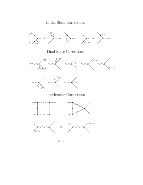
Figure 1: Virtual and real $O(\alpha)$ QED corrections to the process $e^{+}e^{-}\to\pi^{+}\pi^{-}$, excluding vacuum polarization diagrams. The dots stand for the remaining IFS interference correction diagrams.

Let us now consider the radiative corrections to the Born process which are related to additional virtual and real photons. These kind of corrections have been extensively studied in the literature at the one-loop level BonneauMartin ; Tsai ; BerendsKleiss ; Eidelman78 and have been applied in the past by experiments in $e^{+}e^{-}$ cross section measurements. More recently radiative corrections to pion–pair production have been reconsidered in Arbuzov:1997je and were applied by the CMD-2 Collaboration for the determination of the pion form factor Akhmetshin:1999uj ; Akhmetshin:2001ig . For our purpose, we found it necessary to redo these calculations for the $\pi^{+}\pi^{-}$ production channel. To estimate the importance of the different QED correction contributions we begin with an analysis of the cross sections without kinematical cuts for the total cross section $\sigma$ and the pion invariant mass distribution $d\sigma/ds^{\prime}$. Here only IS and FS corrections have to be taken into account since as a consequence of charge conjugation invariance of the electromagnetic interaction the IFS interference corrections do not contribute to these observables.

The IS corrections include the $O(\alpha^{2})$ Berends:1988ab and the leading log $O(\alpha^{3})$ Montagna:1997jv photonic corrections as well as the contributions from initial state fermion pair production Berends:1988ab ; Kniehl:1988id ; Arbuzov:1999uq ; Skrzypek:acta (see Fig. 2). Among the latter only $e^{+}e^{-}$ pair production is numerically relevant.

Figure 2: Initial state fermion pair production. Diagram $a)$ shows an example of a non-singlet contribution, $f^{+}f^{-}$ being a fermion pair which is radiated off the initial state electron or positron. For $f=e$ also singlet contributions like diagram $b)$ have to be taken into account.

The FS corrections are given to $O(\alpha)$ where the pion masses are kept everywhere. Yennie-Frautschi-Suura resummation Bloch:1937pw ; Yennie:1961ad was applied to the IS and FS soft photon contributions. We then obtain ($z=s^{\prime}/s$):

$$\frac{d\sigma}{ds^{\prime}} = \left(\frac{d\sigma}{ds^{\prime}}\right)_{ini}+\left(\frac{d\sigma}{ds^{\prime}}\right)_{fin}\;,$$ (16)

$$\left(\frac{d\sigma}{ds^{\prime}}\right)_{ini} = \frac{\sigma_{0}(s^{\prime})}{s}\biggl{\{}\left[1+\tilde{\delta}_{ini}^{V+S}(s)\right]$$ (17)

$$\times B_{e}(s)\left[1-z\right]^{B_{e}(s)-1}+\tilde{\delta}^{H}_{ini}(s,s^{\prime})\biggr{\}}\;,$$

$$\left(\frac{d\sigma}{ds^{\prime}}\right)_{fin} = \frac{\sigma_{0}(s)}{s}\biggl{\{}\left[1+\tilde{\delta}_{fin}^{V+S}(s)\right]$$

$$\times B_{\pi}(s,s^{\prime})\left[1-z\right]^{B_{\pi}(s,s^{\prime})-1}+\tilde{\delta}^{H}_{fin}(s,s^{\prime})\biggr{\}}\;,$$

with

$$B_{e}(s) = \frac{2\alpha}{\pi}\left[L_{e}-1\right]\;,$$ (19)

$$B_{\pi}(s,s^{\prime}) = \frac{2\alpha}{\pi}\frac{s^{\prime}\beta_{\pi}(s^{\prime})}{s\beta_{\pi}(s)}\;\times$$ (20)

$$\left[\frac{1+\beta_{\pi}^{2}(s^{\prime})}{2\beta_{\pi}(s^{\prime})}\log\left(\frac{1+\beta_{\pi}(s^{\prime})}{1-\beta_{\pi}(s^{\prime})}\right)-1\right]\;,$$

$$\tilde{\delta}_{ini}^{V+S}(s) = \tilde{\delta}_{ini}^{V+S(1)}(s)+\tilde{\delta}_{ini}^{V+S(2)}(s)+\tilde{\delta}_{ini}^{V+S(3)}(s),$$ (21)

$$\tilde{\delta}_{ini}^{V+S(1)}(s) = \frac{\alpha}{\pi}\left[-2+\frac{\pi^{2}}{3}+\frac{3}{2}L_{e}\right]\;,$$ (22)

$$\tilde{\delta}_{ini}^{V+S(2)}(s) = \left(\frac{\alpha}{\pi}\right)^{2}\left[L_{e}^{2}\left(\frac{9}{8}-\frac{\pi^{2}}{3}\right)\right.$$ (23)

$$+ \left.L_{e}\left(-\frac{45}{16}+\frac{11}{12}\pi^{2}+3\zeta(3)\right)\right]+\dots\;,$$

$$\tilde{\delta}_{ini}^{V+S(3)} = \left(\frac{\alpha}{\pi}\right)^{3}\;\left(L_{e}-1\right)^{3}\left[\frac{9}{16}-\frac{\pi^{2}}{2}+\frac{8}{3}\zeta(3)\right],$$ (24)

$$\tilde{\delta}_{ini}^{H}(s,s^{\prime}) = \tilde{\delta}_{ini}^{H(1)}(s,s^{\prime})+\tilde{\delta}_{ini}^{H(2)}(s,s^{\prime})+\tilde{\delta}_{ini}^{H(3)}(s,s^{\prime})$$ (25)

$$+ \tilde{\delta}_{ini}^{pp(2)}(s,s^{\prime})+\tilde{\delta}_{ini}^{pp(3)}(s,s^{\prime})\;,$$

$$\tilde{\delta}_{ini}^{H(1)}(s,s^{\prime}) = -\frac{\alpha}{\pi}\;(1+z)\left(L_{e}-1\right)\;,$$ (26)

$$\tilde{\delta}_{ini}^{H(2)}(s,s^{\prime}) = \left(\frac{\alpha}{\pi}\right)^{2}\left\{L_{e}^{2}\left[-\frac{1+z^{2}}{1-z}\log z\right.\right.$$ (27)

$$+ (1+z)\left(-2\log(1-z)+\frac{\log z}{2}\right)$$

$$- \left.\frac{5}{2}-\frac{z}{2}\right]+L_{e}\biggl{[}\frac{1+z^{2}}{1-z}$$

$$\times \biggl{(}\mbox{Li}_{2}(1-z)+\log z\log(1-z)$$

$$+ \frac{7}{2}\log z-\frac{1}{2}\log^{2}z\biggr{)}+(1+z)$$

$$\times \biggl{(}\frac{1}{4}\log^{2}z+4\log(1-z)-\frac{\pi^{2}}{3}\biggr{)}$$

$$- \left.\log z+7+\frac{z}{2}\biggr{]}\right\}+\dots\;,$$

$$\tilde{\delta}_{ini}^{H(3)}(s,s^{\prime}) = \left(\frac{\alpha}{\pi}\right)^{3}\;\left(L_{e}-1\right)^{3}\;\frac{1}{6}\;\biggl{\{}-\frac{27}{2}$$ (28)

$$+ \frac{15}{4}(1-z)+2(1+z)\Bigl{[}\pi^{2}$$

$$- 6\log^{2}(1-z)+3\mbox{Li}_{2}(1-z)\Bigr{]}$$

$$+ 3\log z\left(\frac{11}{2}-\frac{6}{1-z}+\frac{3}{2}z\right)$$

$$+ \log^{2}z\left(-\frac{7}{2}+\frac{4}{1-z}-\frac{7}{2}z\right)$$

$$- 6\log(1-z)(5+z)+6\log z\log(1-z)$$

$$\times \left(3-\frac{4}{1-z}+3z\right)\biggr{\}},$$

$$\tilde{\delta}_{ini}^{pp(2)} = \theta(s-s^{\prime}-4\;m_{e}\sqrt{s})$$ (29)

$$\times \left[\;\tilde{\delta}_{ini}^{NSin(2)}+\tilde{\delta}_{ini}^{Sin(2)}+\tilde{\delta}_{ini}^{Int(2)}\right]\;,$$

$$\tilde{\delta}_{ini}^{NSin(2)} = \left(\frac{\alpha}{\pi}\right)^{2}\frac{1}{3}\biggl{\{}\frac{1+z^{2}}{2(1-z)}L_{e}^{2}+\biggl{[}\frac{1+z^{2}}{1-z}$$ (30)

$$\times \left(\log\frac{(1-z)^{2}}{z}-\frac{5}{3}\right)-2(1-z)\biggr{]}$$

$$\times L_{e}+\frac{1+z^{2}}{1-z}\left[\frac{1}{2}\log^{2}\frac{(1-z)^{2}}{z}\right.$$

$$- \left.\frac{5}{3}\log\frac{1-z}{z}-\frac{\pi^{2}}{3}+\frac{28}{9}\right]-(1-z)$$

$$\times \left[2\log\frac{(1-z)^{2}}{z}-\frac{19}{3}\right]-\frac{z^{2}}{1-z}$$

$$\times \left[\frac{1}{2}\log^{2}z+\mbox{Li}_{2}(1-z)\right]-\log z\biggr{\}}\;,$$

$$\tilde{\delta}_{ini}^{Sin(2)} = \left(\frac{\alpha}{\pi}\right)^{2}\biggl{\{}\left[\frac{1}{2}(1+z)\log z+\frac{1}{3z}+\frac{1}{4}\right.$$ (31)

$$- \frac{1}{4}z-\left.\frac{1}{3}z^{2}\right]L_{e}^{2}+\biggl{[}(1+z)\Bigl{(}2\log z$$

$$\times \log(1-z)-\log^{2}z+2\mbox{Li}_{2}(1-z)\Bigr{)}$$

$$+ \Bigl{(}\frac{4}{3z}+1-z-\frac{4}{3}z^{2}\Bigr{)}\log(1-z)$$

$$- \left(\frac{2}{3z}+1-\frac{1}{2}z-\frac{4}{3}z^{2}\right)\log z-\frac{8}{9z}-\frac{8}{3}$$

$$+ \frac{8}{3}z+\frac{8}{9}z^{2}\biggr{]}L_{e}\biggr{\}}+\dots\;,$$

$$\tilde{\delta}_{ini}^{Int(2)} = \left(\frac{\alpha}{\pi}\right)^{2}\left\{\frac{1+z^{2}}{1-z}\left[-\mbox{Li}_{2}(1-z)-\frac{1}{2}\log^{2}z\right.\right.$$ (32)

$$- \left.\left.\frac{3}{4}\log z\right]-\frac{7}{4}(1+z)\log z-4+\frac{7}{2}z\right\}\;L_{e}$$

$$+ \dots\;,$$

$$\tilde{\delta}_{ini}^{pp(3)} = \theta(s-s^{\prime}-4\;m_{e}\sqrt{s})$$ (33)

$$\times \left[\tilde{\delta}_{ini}^{NSin(3)}+\tilde{\delta}_{ini}^{Sin(3)}+\tilde{\delta}_{ini}^{Int(3)}\right]\;,$$

$$\tilde{\delta}_{ini}^{NSin(3)} = \biggl{(}\frac{\alpha}{\pi}\biggr{)}^{3}L_{e}\biggl{[}\frac{1+z^{2}}{1-z}\,L_{e}^{2}$$ (34)

$$\times \biggl{(}\frac{2}{3}\log(1-z)-\frac{1}{3}\log z+\frac{1}{2}\biggr{)}$$

$$+ L_{e}^{2}\biggl{(}\frac{1+z}{6}\log z-\frac{1-z}{3}\biggr{)}$$

$$+ \frac{1+z^{2}}{1-z}\,L_{e}\biggl{(}2\log^{2}(1-z)$$

$$- \frac{11}{9}\log(1-z)-\frac{9}{4}-\frac{2}{9}\pi^{2}-2\log z$$

$$\times \log(1-z)+\frac{1}{3}\log^{2}z+\frac{11}{18}\log z\biggr{)}$$

$$+ L_{e}\biggl{(}-\frac{8}{3}(1-z)\log(1-z)$$

$$+ \frac{2}{3}(1+z)\log z\log(1-z)-\frac{1}{6}(1+z)$$

$$\times \log^{2}z+\frac{4}{9}(1-5z)\log z+\frac{2}{3}(1+z)$$

$$\times \mbox{Li}_{2}(1-z)+\frac{19}{9}(1-z)\biggr{)}$$

$$+ \frac{1+z^{2}}{1-z}\biggl{(}\frac{16}{9}\log^{3}(1-z)-\frac{7}{3}\log^{2}(1-z)$$

$$+ \frac{67}{27}\log(1-z)-\frac{8}{9}\pi^{2}\log(1-z)-\frac{8}{3}$$

$$\times \log z\log^{2}(1-z)+\frac{7}{3}\log z\log(1-z)$$

$$+ \frac{5}{6}\log^{2}z\log(1-z)-\frac{1}{3}\mbox{Li}_{2}(1-z)$$

$$\times \log(1-z)-\frac{1}{18}\log^{3}z-\frac{31}{72}\log^{2}z$$

$$- \frac{67}{54}\log z-\frac{2}{3}\mbox{Li}_{2}(1-z)\log z+\frac{4}{9}\pi^{2}$$

$$\times \log z-\frac{1}{4}\mbox{Li}_{2}(1-z)-\frac{5}{3}{\rm S}_{1,2}(1-z)$$

$$- \frac{2}{9}\pi^{2}+4\zeta(3)+\frac{1073}{162}\biggr{)}\biggr{]}\;,$$

$$\tilde{\delta}_{ini}^{Sin(3)} = -\biggl{(}\frac{\alpha}{\pi}\biggr{)}^{3}\;\frac{1}{36}\left(L_{e}-1\right)^{3}\biggl{[}\frac{1-z}{3z}(4$$ (35)

$$+ 7z+4z^{2})+2(1+z)\log z\biggr{]}\;,$$

$$\tilde{\delta}_{ini}^{Int(3)} = \biggl{(}\frac{\alpha}{\pi}\biggr{)}^{3}\;\frac{5}{24}\left(L_{e}-1\right)^{3}\left[\biggl{(}\frac{3}{2}\right.$$ (36)

$$+ 2\log(1-z)\biggl{)}\biggl{(}\frac{1-z}{3z}(4+7z+4z^{2}\biggr{)}$$

$$+ 2(1+z)\log z\biggr{)}+(1+z)\biggl{(}-\log^{2}z$$

$$+ 4\mbox{Li}_{2}(1-z)\biggr{)}+\frac{1}{3}\left(-9-3z+8z^{2}\right)$$

$$\times \left.\log z+\frac{2}{3}\left(-\frac{3}{z}-8+8z+3z^{2}\right)\right]\;,$$

$$\tilde{\delta}_{fin}^{V+S}(s) = \frac{\alpha}{\pi}\left\{\frac{3s-4m_{\pi}^{2}}{s\beta_{\pi}}\;\log\left(\frac{1+\beta_{\pi}}{1-\beta_{\pi}}\right)-2\right.$$ (37)

$$- \frac{1}{2}\;\log\left(\frac{1-\beta_{\pi}^{2}}{4}\right)-\frac{3}{2}\;\log\left(\frac{s}{m_{\pi}^{2}}\right)$$

$$- \frac{1+\beta_{\pi}^{2}}{2\beta_{\pi}}\;\left[\log\left(\frac{1+\beta_{\pi}}{1-\beta_{\pi}}\right)\biggl{[}\log\left(\frac{1+\beta_{\pi}}{2}\right)\right.$$

$$+ \log(\beta_{\pi})\biggr{]}+\log\left(\frac{1+\beta_{\pi}}{2\beta_{\pi}}\right)\log\left(\frac{1-\beta_{\pi}}{2\beta_{\pi}}\right)$$

$$+ 2\mbox{Li}_{2}\left(\frac{2\beta_{\pi}}{1+\beta_{\pi}}\right)+2\mbox{Li}_{2}\left(-\frac{1-\beta_{\pi}}{2\beta_{\pi}}\right)$$

$$- \left.\left.\frac{2}{3}\pi^{2}\right]\right\}\;,$$

$$\tilde{\delta}_{fin}^{H}(s,s^{\prime}) = \frac{2\alpha}{\pi}(1-z)\frac{\beta_{\pi}(s^{\prime})}{\beta_{\pi}^{3}(s)}\;,$$ (38)

$$\mbox{Li}_{2}(x) = -\int\limits_{0}^{x}\frac{\mathop{{\rm d}y}}{y}\log(1-y),$$

$${\mathrm{S}}_{1,2}(x) = \frac{1}{2}\int\limits_{0}^{x}\frac{\mathop{{\rm d}y}}{y}\log^{2}(1-y)\;,\;L_{e}=\log\left(\frac{s}{m_{e}^{2}}\right).$$

The $O(\alpha^{3})$ corrections (24), (28) and (33) are taken from Montagna:1997jv and Arbuzov:1999uq ; Skrzypek:acta respectively. The dots in (23), (27), (31) and (32) correspond to $O(\alpha^{2})$ contributions which do not contain any $\log(s/m_{e}^{2})$ terms and can be neglected safely.

Figure 3: Pion pair invariant mass distributions ($d\sigma/ds^{\prime}$) with radiative corrections, normalized to $d\sigma/ds^{\prime}$ with only $O(\alpha)$ IS corrections. The thick line shows the case when up to $O(\alpha^{2})$ IS and $O(\alpha)$ FS contributions (excluding IS pair production) are taken into account and appropriately resummed [see (16-2)]. The thin solid line shows the same but this time without resummation. The dotted line corresponds to the $O(\alpha)$ FS corrections (together with $O(\alpha)$ IS corrections). For the long-dashed and the dot-dashed lines only the resummed IS $O(\alpha^{2})$ and the resummed IS $O(\alpha)$ radiative corrections are taken into account, respectively.

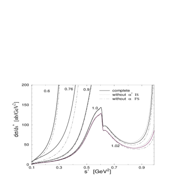
Figure 4: Pion pair invariant mass distributions ($d\sigma/ds^{\prime}$) for different center of mass energies $\sqrt{s}=0.6,0.76,0.9,1.0,1.02$ GeV. The solid lines stands for the “complete” cross section, including $O(\alpha^{2})$ IS and $O(\alpha)$ FS corrections [see (16-2)]. The dotted lines give the results when the $O(\alpha^{2})$ IS corrections are neglected. The dot-dashed lines correspond to the case when the $O(\alpha)$ FS contribution is neglected.

Fig. 3 shows the pion pair invariant mass distributions $d\sigma/ds^{\prime}$ with radiative corrections normalized to $d\sigma/ds^{\prime}$ with only $O(\alpha)$ IS corrections ($\sqrt{s}=1.02$ GeV). In Table 2 the contribution from IS $O(\alpha^{2})$ and FS $O(\alpha)$ photonic corrections are shown for different center of mass energies.

The following points can be recognized:

1. The FS corrections (dotted line) are quite large, especially in the region of soft photons as well as for very hard photons;

2. The $O(\alpha^{2})$ IS effects are considerable;

3. The FS and IS contributions compensate each other significantly for large $s^{\prime}$.

Fig. 4 shows $d\sigma/ds^{\prime}$ for different center of mass energies $\sqrt{s}$. Going to smaller center of mass energies the $O(\alpha^{2})$ IS corrections become smaller and smaller. On the other hand the FS contributions remain considerably large. Interestingly, for the $\phi$ resonance energy ($\sqrt{s}=1.02$ GeV) both the $O(\alpha^{2})$ IS and the $O(\alpha)$ FS contributions are large. Quantitatively this is shown in Table 2. The resummation of the $O(\alpha^{2})$ IS soft photon logarithms [see (17)] gives a contribution smaller than 5 per mill for $s^{\prime}$ below the $\rho$ resonance peak and smaller than 3 per mill above it. The resummation of FS soft photon logarithms [see (2)] changes the complete results only slightly (less than 0.5 per mill).

$\sqrt{s^{\prime}}\;[\mbox{GeV}]$	$O(\alpha^{2})$ IS	$O(\alpha)$ FS
	contribution	contribution
0.3	4.3	11.5
0.4	4.4	4.3
0.5	4.0	3.2
0.6	3.4	2.0
0.7	2.2	0.9
0.76	1.2	0.7
0.8	0.2	1.2
0.9	$-$ 3.6	5.5
0.95	$-$ 6.9	10.1
1.0	$-$ 15.3	16.6

Table 2: Contribution of $O(\alpha^{2})$ IS and $O(\alpha)$ FS corrections to $d\sigma/ds^{\prime}$ (in %), $\sqrt{s}=1.02$ GeV.

To reduce the theoretical error to a few per mill one also has to include the contributions from initial state $e^{+}e^{-}$ pair production Berends:1988ab ; Kniehl:1988id ; Arbuzov:1999uq ; Skrzypek:acta , given in (29) and (33). In Table 3 and 4 the $O(\alpha^{2})$ and leading $O(\alpha^{3})$ pair production contributions to $d\sigma/ds^{\prime}$ for different hadronic energies are presented. What is remarkable is the very large singlet contribution [see Fig. 2b)] in the region of low hadronic energies which amounts about 8 per cent for $\sqrt{s^{\prime}}=0.3$ GeV. Since these effects are related to $e^{+}e^{-}$ pairs which are mainly emitted collinearly to the beam axis they escape detection and therefore have to be included into the data analysis. Hence when unfolding the data from radiative corrections also these effects have to be subtracted. The leading contribution from $O(\alpha^{3})$ pair production appears to be less than $1$ per mill which gives us a good estimate about the precision we can expect.

We also take into accout the leading log $O(\alpha^{3})$ IS photon correction Montagna:1997jv , which is given in (24) and (28). The contribution can be of the order of $4$ per mill for hadronic energies below the $\rho$ resonance peak, as shown in Table 5.

$\sqrt{s^{\prime}}$ [GeV]	$O(\alpha^{2})$ IS pp	Singlet
	contribution	contribution
0.3	79.1	74.9
0.4	36.3	31.9
0.5	16.6	12.2
0.6	8.3	4.0
0.7	4.8	0.76
0.76	3.9	$-$ 0.01
0.8	3.4	$-$ 0.24
0.9	2.7	$-$ 0.27
1.0	1.2	0.06

Table 3: $O(\alpha^{2})$ contribution from IS pair production to $d\sigma/ds^{\prime}$ (in per mill). In the second column only the singlet contribution (including singlet-non-singlet interference) is shown.

$\sqrt{s^{\prime}}$ [GeV]	$O(\alpha^{3})$ IS pp	Singlet
	contribution	contribution
0.3	$-$ 0.87	$-$ 1.27
0.4	$-$ 0.45	$-$ 0.82
0.5	$-$ 0.18	$-$ 0.48
0.6	$-$ 0.07	$-$ 0.27
0.7	$-$ 0.09	$-$ 0.15
0.76	$-$ 0.15	$-$ 0.10
0.8	$-$ 0.21	$-$ 0.07
0.9	$-$ 0.43	$-$ 0.03
1.0	$-$ 0.72	$-$ 0.001

Table 4: $O(\alpha^{3})$ IS pair production contribution to $d\sigma/ds^{\prime}$ (in per mill).

$\sqrt{s^{\prime}}$ [GeV]	$O(\alpha^{3})$ IS
	contribution
0.3	3.9
0.4	4.3
0.5	4.2
0.6	3.8
0.7	3.0
0.76	2.4
0.8	1.8
0.9	0.3
1.0	0.6

Table 5: $O(\alpha^{3})$ leading log IS photon contribution to $d\sigma/ds^{\prime}$ (in per mill).

The total cross section $\sigma(s)$ can be obtained by carrying out the $s^{\prime}$ integration in (16) numerically. For $\sigma(s)$ the $O(\alpha^{2})$ IS corrections are not as important as for $d\sigma/ds^{\prime}$ (they account for at most $1\,\%$, at $\sqrt{s}=1.02$ GeV 2 per mill). Neglecting the $O(\alpha^{2})$ corrections, $\sigma(s)$ can then be written in the following simple form:

$$\sigma(s) = \sigma_{0}\left[1+\delta_{ini}(\Lambda)+\delta_{fin}(\Lambda)\right]$$

$$+ \int_{4m_{\pi}^{2}}^{s-2\sqrt{s}\Lambda}ds^{\prime}\;\sigma_{0}(s^{\prime})\rho_{ini}(s,s^{\prime})$$

$$+ \sigma_{0}(s)\int_{4m_{\pi}^{2}}^{s-2\sqrt{s}\Lambda}ds^{\prime}\;\rho_{fin}(s,s^{\prime})\;,$$

with

$$\delta_{ini}(\Lambda) = \log\left(\frac{2\Lambda}{\sqrt{s}}\right)\>B_{e}(s)+\tilde{\delta}_{ini}^{V+S(1)}(s)\;,$$ (40)

$$\delta_{fin}(\Lambda) = \log\left(\frac{2\Lambda}{\sqrt{s}}\right)\>B_{\pi}(s,s^{\prime})+\tilde{\delta}_{fin}^{V+S(1)}(s)\;,$$ (41)

$$\rho_{ini}(s,s^{\prime}) = \frac{1}{s}\left[\tilde{\delta}_{ini}^{H(1)}(s,s^{\prime})+\frac{B_{e}(s)}{1-z}\right]\;,$$ (42)

$$\rho_{fin}(s,s^{\prime}) = \frac{1}{s}\left[\tilde{\delta}_{fin}^{H}(s,s^{\prime})+\frac{B_{\pi}(s,s^{\prime})}{1-z}\right]\;,$$ (43)

where $\Lambda$ is the soft photon cut off energy which drops out in the sum (2).

The total cross section is plotted in Fig. 5. In Table 6 the $O(\alpha)$ FS corrections to $\sigma(s)$ for different center of mass energies are shown. Although it can be hardly recognized directly from the figure, the FS contributions are not marginal for energies below the $\rho$ resonance peak.

Figure 5: Total cross section $\sigma(s)$ as a function of the center of mass energy. The solid line corresponds to $\sigma(s)$ as given in (2). The dotted line corresponds to the Born cross section. The dot-dashed line corresponds to the Born cross section with only $O(\alpha)$ IS corrections.

$\sqrt{s}$ [GeV]	$O(\alpha)$ FS
	contribution
0.3	3.6
0.4	1.2
0.5	0.9
0.6	0.9
0.76	0.7
0.9	0.4
1.02	0.3

Table 6: Contribution of $O(\alpha)$ FS corrections to the total cross section (in %).

Taking the high energy limit in (2) provides a good cross check for the FS correction results. Carrying out the $s^{\prime}$ integration for $s\to\infty$ and adding this result to the high energy virtual and soft photon FS corrections leads to an expression in which the $s$ dependence drops out. This has to be the case according to the Kinoshita-Lee-Nauenberg theorem Kinoshita:1962ur ; Lee:1964is which requires the collinear logarithms to cancel. In addition all terms proportional to $\pi^{2}$ drop out. Defining

$$\eta(s) \equiv \frac{\pi}{\alpha}\left[\delta_{fin}(\Lambda)+\int_{4m_{\pi}^{2}}^{s-2\sqrt{s}\Lambda}ds^{\prime}\;\rho_{fin}(s,s^{\prime})\right]\;,$$ (44)

one can write the total cross section with only $O(\alpha)$ FS corrections in the following compact way:

$$\sigma_{fin}(s) = \left[1+\eta(s)\frac{\alpha}{\pi}\right]\sigma_{0}(s)\;.$$ (45)

The function $\eta(s)$ is given by Schwinger:1989ix ; Drees:1990te ; Melnikov:2001uw

$$\begin{array}[]{l}\eta(s)=\frac{1+\beta_{\pi}^{2}}{\beta_{\pi}}\Biggl{\{}4{\rm Li}_{2}\left(\frac{1-\beta_{\pi}}{1+\beta_{\pi}}\right)+2{\rm Li}_{2}\left(-\frac{1-\beta_{\pi}}{1+\beta_{\pi}}\right)\\ -3\log\left(\frac{2}{1+\beta_{\pi}}\right)\>\log\left(\frac{1+\beta_{\pi}}{1-\beta_{\pi}}\right)-2\log(\beta_{\pi})\>\log\left(\frac{1+\beta_{\pi}}{1-\beta_{\pi}}\right)\Biggr{\}}\\ -3\log\left(\frac{4}{1-\beta_{\pi}^{2}}\right)-4\log(\beta_{\pi})\\ +\frac{1}{\beta_{\pi}^{3}}\left[\frac{5}{4}(1+\beta_{\pi}^{2})^{2}-2\right]\>\log\left(\frac{1+\beta_{\pi}}{1-\beta_{\pi}}\right)+\frac{3}{2}\frac{1+\beta_{\pi}^{2}}{\beta_{\pi}^{2}}\end{array}$$ (47)

and provides a good measure for the dependence of the observables on the pion mass. Neglecting the pion mass is obviously equivalent to taking the high energy limit. In this limit we observe:

$$\eta(s\to\infty) = 3\;.$$ (48)

Our result in (48) agrees with the result obtained by Schwinger Schwinger:1989ix but disagrees with that in Arbuzov:1997je for which in this limit the terms $\propto\pi^{2}$ do not drop out. In Fig. 6 $\eta(s)$ is plotted as a function of the center of mass energy. It can be realized that for energies below 1 GeV the pion mass leads to a considerable enhancement of the FS corrections. Regarding the desired precision, ignoring the pion mass would therefore lead to wrong results.

Close to threshold for pion pair production ($s\simeq 4m_{\pi}^{2}$) the Coulomb forces between the two final state pions play an important role. In this limit the factor $\eta(s)$ becomes singular [$\eta(s)\to\pi^{2}/2\beta_{\pi}$] which means that the $O(\alpha)$ result for the FS correction cannot be trusted anymore. Since these singularities are known to all orders of perturbation theory one can resum these contribution, which leads to an exponentiation Schwinger:1989ix :

$$\sigma_{fin}(s) = \sigma_{0}\;\left(1+\eta(s)\frac{\alpha}{\pi}-\frac{\pi\alpha}{2\beta_{\pi}}\right)\;\frac{\pi\alpha}{\beta_{\pi}}$$ (49)

$$\times\left[1-\exp\left(-\frac{\pi\alpha}{\beta_{\pi}}\right)\right]^{-1}\;\;.$$

Above a center of mass energy of $\sqrt{s}=0.3\;\mbox{GeV}$ the exponentiated correction to the Born cross section deviates from the non-exponentiated correction less than $1\,\%$.

Figure 6: The FS correction factor $\eta(s)$ as a function of the center of mass energy $\sqrt{s}$ [see (44-48)].

We now consider the IFS interference corrections (see Fig. 1) which modify the angular distribution. To $O(\alpha)$ we can write:

$$\left(\frac{d\sigma}{d\Omega}\right) = \left(\frac{d\sigma_{0}}{d\Omega}\right)\;\Bigl{[}1+\delta(\Lambda)\Bigr{]}$$

$$+ \left(\frac{d\sigma_{h}}{d\Omega}\right)(\Lambda)\;,$$

where the correction factor $\delta$ is the sum of the virtual plus soft photon IS, FS and IFS interference correction factors:

$$\delta(\Lambda) = \delta_{ini}(\Lambda)+\delta_{fin}(\Lambda)+\delta_{int}(\Lambda)\;.$$ (51)

$d\sigma_{h}/d\Omega$ is the hard photon contribution which is calculated numerically. $\delta_{ini}(\Lambda)$ and $\delta_{fin}(\Lambda)$ are given in (40) and (41). $\delta_{int}(\Lambda)$ can be written in the following, compact way:

$$\delta_{int} = \frac{2\alpha}{\pi}\Biggl{\{}\log\left(\frac{-u+m_{\pi}^{2}}{-t+m_{\pi}^{2}}\right)\log\left(\frac{4\Lambda^{2}}{s}\right)$$ (52)

$$+ \frac{1}{4}\frac{s^{2}}{ut-m_{\pi}^{4}}\biggl{\{}\frac{u-t}{s}\Bigl{[}c_{1}(u)+c_{1}(t)+c_{e}+c_{\pi}\Bigr{]}$$

$$+ \frac{u+t}{s}\Bigl{[}c_{1}(u)-c_{1}(t)\Bigr{]}\biggr{\}}\;-\;\frac{F(u)}{2}+\frac{F(t)}{2}\Biggr{\}},$$

with ($x=u,t$, $\kappa_{i}=\kappa_{i}(x)$)

$$c_{1}(x) = \frac{1}{2}\biggl{\{}3\log^{2}\left(\frac{x-m_{\pi}^{2}}{x}\right)-\frac{1}{2}\log^{2}\left(-\frac{m_{e}^{2}}{x}\right)$$

$$- \frac{1}{2}\log^{2}\left(-\frac{m_{\pi}^{2}}{x}\right)-2\log\left(-\frac{m_{\pi}^{2}}{x}\right)\log\left(\frac{x-m_{\pi}^{2}}{x}\right)$$

$$+ 2\mbox{Li}_{2}\left(-\frac{m_{\pi}^{2}}{x-m_{\pi}^{2}}\right)-\frac{\pi^{2}}{3}\biggr{\}}\;,$$

$$c_{\pi} = \frac{1+\beta_{\pi}^{2}}{2\beta_{\pi}}\left[2\mbox{Li}_{2}\left(\frac{1+\beta_{\pi}}{2}\right)-2\mbox{Li}_{2}\left(\frac{1-\beta_{\pi}}{2}\right)\right.$$

$$\;+\mbox{Li}_{2}\left(-\frac{1+\beta_{\pi}}{1-\beta_{\pi}}\right)-\mbox{Li}_{2}\left(-\frac{1-\beta_{\pi}}{1+\beta_{\pi}}\right)$$

$$\left.\;+\log\left(\frac{s}{m_{\pi}^{2}}\right)\log\left(\frac{1+\beta_{\pi}}{1-\beta_{\pi}}\right)\right]\;,$$

$$c_{e} = \frac{1}{2}\log^{2}\left(\frac{s}{m_{e}^{2}}\right)+\frac{\pi^{2}}{6}\;,$$

$$F(x) = \left[f_{1}^{x}(\kappa_{1})-f_{1}^{x}(\kappa_{2})-f_{1}^{x}(\kappa_{4})+f_{2}^{x}(\kappa_{3})\right.$$

$$- f_{3}^{x}(\kappa_{1},\kappa_{2})-f_{3}^{x}(\kappa_{4},\kappa_{1})+f_{3}^{x}(\kappa_{4},\kappa_{2})$$

$$+ f_{4}^{x}(\kappa_{2},\kappa_{1})+f_{4}^{x}(\kappa_{1},\kappa_{4})+f_{4}^{x}(\kappa_{2},\kappa_{4})$$

$$- f_{5}^{x}(\kappa_{3},\kappa_{1})+f_{5}^{x}(\kappa_{3},\kappa_{2})-f_{5}^{x}(\kappa_{3},\kappa_{4})$$

$$- \left.f_{6}^{x}(\kappa_{1},\kappa_{3})-f_{6}^{x}(\kappa_{2},\kappa_{3})+f_{6}^{x}(\kappa_{4},\kappa_{3})\right],$$

$$f_{1}^{x}(\eta) = \frac{1}{2}\log^{2}[b_{x}-\eta]-\frac{1}{2}\log^{2}[a-\eta],$$

$$f_{2}^{x}(\eta) = \frac{1}{2}\log^{2}[\eta-a]-\frac{1}{2}\log^{2}[\eta-b_{x}],$$

$$f_{3}^{x}(\eta_{1},\eta_{2}) = -\mbox{Li}_{2}\left[\frac{(b_{x}-a)(\eta_{1}-\eta_{2})}{(b_{x}-\eta_{1})(a-\eta_{2})}\right]$$

$$+ \mbox{Li}_{2}\left(-\frac{b_{x}-a}{a-\eta_{2}}\right)+\mbox{Li}_{2}\left(\frac{b_{x}-a}{b_{x}-\eta_{1}}\right)$$

$$+ \log(b_{x}-\eta_{1})\log\left(\frac{b_{x}-\eta_{2}}{a-\eta_{2}}\right),$$

$$f_{4}^{x}(\eta_{1},\eta_{2}) = \mbox{Li}_{2}\left[\frac{(b_{x}-a)(\eta_{2}-\eta_{1})}{(b_{x}-\eta_{2})(a-\eta_{1})}\right],$$

$$- \mbox{Li}_{2}\left(-\frac{b_{x}-a}{a-\eta_{1}}\right)-\mbox{Li}_{2}\left(\frac{b_{x}-a}{b_{x}-\eta_{2}}\right)$$

$$+ \log(a-\eta_{1})\log\left(\frac{b_{x}-\eta_{2}}{a-\eta_{2}}\right),$$

$$f_{5}^{x}(\eta_{1},\eta_{2}) = \log[\eta_{1}-\eta_{2}]\log\left(\frac{b_{x}-\eta_{2}}{a-\eta_{2}}\right)$$

$$+ \mbox{Li}_{2}\left(\frac{a-\eta_{2}}{\eta_{1}-\eta_{2}}\right)-\mbox{Li}_{2}\left(\frac{b_{x}-\eta_{2}}{\eta_{1}-\eta_{2}}\right),$$

$$f_{6}^{x}(\eta_{1},\eta_{2}) = \log[\eta_{2}-\eta_{1}]\log\left(\frac{\eta_{2}-b_{x}}{\eta_{2}-a}\right)$$

$$+ \mbox{Li}_{2}\left(\frac{\eta_{2}-a}{\eta_{2}-\eta_{1}}\right)-\mbox{Li}_{2}\left(\frac{\eta_{2}-b_{x}}{\eta_{2}-\eta_{1}}\right),$$

$$a=\beta_{\pi}(s)\;,\quad b_{x}=\beta_{e}(s)+2\sqrt{-\frac{x}{s}},$$

$$\kappa_{1,2}\equiv\kappa_{1,2}(x) = -1+\frac{1}{\sqrt{-sx}}\Bigl{[}-x+m_{e}^{2}-m_{\pi}^{2}$$

$$\pm \sqrt{\lambda(x,m_{e}^{2},m_{\pi}^{2})}\Bigr{]},$$

$$\kappa_{3,4}\equiv\kappa_{3,4}(x) = 1+\frac{1}{\sqrt{-sx}}\Bigl{[}-x+m_{e}^{2}-m_{\pi}^{2}$$

$$\pm \sqrt{\lambda(x,m_{e}^{2},m_{\pi}^{2})}\Bigr{]},$$

$$\lambda(x,y,z) = z^{2}+y^{2}+z^{2}-2xy-2xz-2yz.$$

From (52) it can be seen immediately that $\delta_{int}$ is antisymmetric, thus it changes sign under the exchange $t\leftrightarrow u$ [$t(u)=(p_{1}-k_{2(1)})^{2}$]. This is actually required by charge conjugation invariance.

Figure 7: $\pi^{-}$ angular distribution for $\sqrt{s}=1.02$ GeV. The solid line, corresponding to the complete $O(\alpha)$ corrections, is not symmetric as a consequence of the IFS interference corrections. Both the tree level distribution and the distribution with only IS and FS corrections are symmetric.

$\cos{\Theta}$	$\frac{d\sigma_{B+IS+FS}}{d\cos\Theta}/\frac{d\sigma_{tot}}{d\cos\Theta}$	IFS interference
$-$1.0	0.99/ 1.46	47.5
$-$0.99	2.95/3.33	12.9
$-$0.94	11.12/11.74	5.6
$-$0.6	44.03/44.97	2.1
$-$0.2	59.91/60.3	0.6
0.	61.76/ 61.76	0.0
0.2	59.91/ 59.53	$-$0.6
0.6	44.03/43.09	$-$2.1
0.94	11.12/10.49	$-$5.6
0.99	2.95/2.56	$-$13.2
1.0	0.99/ 0.52	$-$47.5

Table 7: Contribution of the interference terms (in %) to the differential cross section (corresponding to the solid and dotted line in Fig. 7).

Figure 8: Lowest order $\pi^{-}$ angular distribution for the case of a tagged photon. The angular cut between the photon momentum and the beam axis is chosen such that only photons in the angular range $60^{o}\leq\Theta_{\gamma}\leq 120^{o}$ are detected. The difference between the solid and dotted line is due to an additional cut between the tagged photon and the pions $7^{o}\leq\Theta_{\gamma\pi}\leq 173^{o}$ (solid line). This cut was also applied to the remaining dashed and dot-dashed line. The curves correspond to different values for the minimal photon energy $\Lambda$. The solid and the dotted line correspond to $\Lambda=0.01$ GeV, the dashed line to $\Lambda=0.02$ GeV and the dot-dashed line to $\Lambda=0.03$ GeV.

Table 7 shows the IFS interference contribution to the pion angular distribution (Fig. 7). One can recognize, that with an angular cut between the pion momentum and the beam axis of $20^{o}\leq\Theta\leq 160^{o}$ this is not bigger than $5.6\,\%$. The importance of the interference contribution can be enhanced by tagging the photon and imposing a strong cut on the angle between the photon momentum and the beam axis Binner:1999bt (see Fig. 8). This seems to be the only way to tackle the imaginary part of the pion form factor.

Figure 9: Pion pair invariant mass distribution with an angular cut $30^{o}\leq\Theta\leq 150^{o}$ between the $\pi^{\pm}$ momenta and the beam axis, $\sqrt{s}=1.02$ GeV.

The results presented so far have been obtained by the dedicated Fortran program A$\phi\rho\omega$dite . It generates cross sections with the option of kinematical cuts Hoefer:2001dr as needed by experiment. As shown before, the $O(\alpha^{2})$ IS (photonic and IS pair production) contributions to $d\sigma/ds^{\prime}$ are considerable and even $O(\alpha^{3})$ leading log contributions should be included. Analytical formulae for the full $O(\alpha^{2})$ IS corrections with cuts have not been calculated so far. At this stage we therefore rely on the complete results without cuts $d\sigma^{(compl)}/ds^{\prime}$ as given in (16) with the following approximation:

$$\left(\frac{d\sigma^{(\rm compl)}}{ds^{\prime}}\right)_{\rm cuts}\simeq\frac{\left(\frac{d\sigma^{(\rm compl)}}{ds^{\prime}}\right)_{\rm no\;cuts}}{\left(\frac{d\sigma^{(\alpha)}}{ds^{\prime}}\right)_{\rm no\;cuts}}\left(\frac{d\sigma^{(\alpha)}}{ds^{\prime}}\right)_{\rm cuts}.$$ (53)

$d\sigma^{(\alpha)}/ds^{\prime}$ is the differential cross section to $O(\alpha)$. See Fig. 9 for an example. In the limit $s^{\prime}\to s$ the above approximation is exact since then the radiated photons are soft. In principle we can expect that away from this limit the situation is different since the contribution from a second hard photon could distort the angular distribution of the pions. The distortion however remains below 1 per mill for $s^{\prime}\geq 0.3$ $\mbox{GeV}^{2}$ and an angular cut between the pion momenta and the beam axis of less than 30 degrees.

In the case of a tagged photon the FS corrections can be reduced by applying strong cuts between the photon and the final state particles. See Fig. 10 for such a strong cut scenario at the $\phi$ peak. It can be seen that the strong cuts reduce the FS contribution considerably. However, as shown in Table 8, the FS contribution still amounts up to a few per cent. Although the presented results are based on an $O(\alpha)$ calculation (a similar approximation as the one given in (53) is not possible) it is highly unprobable that the situation will improve if $O(\alpha^{2})$ corrections are included.

Figure 10: Pion pair invariant mass distribution $d\sigma/ds^{\prime}$ for the case of a tagged photon. Set A corresponds to a $7^{o}$ angular cut between the photon momentum and the beam axis and a $30^{o}$ cut between the $\pi^{\pm}$ momenta and the beam axis. For set B the pion cuts are the same but the photon cut is now $20^{o}$. Taking the difference (Set A-Set B) the photon is restricted to a region well separated from the pion momenta. The solid lines correspond to the complete cross section (Born plus IS and FS bremsstrahlung), for the dotted lines FS bremsstrahlung is neglected.

s’	Set A		Set B		set A $-$ set B
	all	no FS	all	no FS	all	no FS
0.8	11.994	9.981	18.231	16.121	6.237	6.140
0.85	12.252	9.494	18.201	15.313	5.949	5.819
0.9	14.212	10.168	20.615	16.384	6.403	6.216

Table 8: $d\sigma/ds^{\prime}$ in $[nb/\mbox{GeV}^{2}]$, for some values of $s^{\prime}$. The FS contribution for a strong cut scenario (Set A-Set B) is shown. It is 1.6 %, 2.2 %, 2.9 % for $s^{\prime}=0.8,\;0.85,\;0.9\;\mbox{GeV}^{2}$, respectively.

Finally a few remarks about the A$\phi\rho\omega$dite program. To check the numerical accuracy, the four dimensional phase space integration has been carried out numerically to obtain the total cross section without cuts (see Table 9). This is then compared to the total cross section obtained from (2) by one-dimensional integration (Table 10). We observe excellent agreement. Table 10 and Table 9 in addition show the total cross section as a function of the soft photon energy cut-off $\Lambda$. For values of $\Lambda<10^{-4}$ GeV we get stable cut-independent results.

$\Lambda$ [GeV]	$\sigma$ [nb]	$\delta\sigma$ [nb]
0.1	94.907	0.0095
0.01	99.123	0.0104
0.001	99.394	0.0129
0.0001	99.420	0.0157
$10^{-5}$	99.422	0.0210
$10^{-6}$	99.422	0.0255
$10^{-7}$	99.422	0.0303
$10^{-8}$	99.421	0.0357
$10^{-9}$	99.422	0.0418
$10^{-10}$	99.421	0.0493

Table 9: Cut-off dependence of the total cross section $\sigma$ obtained from 4-dimensional numerical integration, $\sqrt{s}=1.02$ GeV. $\delta\sigma$ is the absolute numerical error to $\sigma$.

$\Lambda$ [GeV]	$\sigma$ [nb]	$\delta\sigma$ [nb]
0.1	94.909344406421	2$\cdot 10^{-9}$
0.01	99.126309344279	$2\cdot 10^{-11}$
0.001	99.396403660854	$2\cdot 10^{-9}$
0.0001	99.422466900996	$3\cdot 10^{-9}$
$10^{-5}$	99.425064117054	$6\cdot 10^{-9}$
$10^{-6}$	99.425323747942	$7\cdot 10^{-9}$
$10^{-7}$	99.425349708976	$7\cdot 10^{-9}$
$10^{-8}$	99.425352318987	$1\cdot 10^{-8}$
$10^{-9}$	99.425352327085	$1\cdot 10^{-8}$
$10^{-10}$	99.425352168781	$1\cdot 10^{-8}$

Table 10: Cut-off dependence of the total cross section $\sigma$ obtained from 1-dimensional numerical integration, $\sqrt{s}=1.02$ GeV. $\delta\sigma$ is the absolute error to $\sigma$

3 The Pion Form Factor from Radiative Return

The pion–pair invariant mass spectrum in scalar QED may be written in the form

$$\frac{d\sigma}{ds^{\prime}}=\left(\frac{d\sigma}{ds^{\prime}}\right)_{\rm ini}+\left(\frac{d\sigma}{ds^{\prime}}\right)_{\rm int}+\left(\frac{d\sigma}{ds^{\prime}}\right)_{\rm fin}\;.$$ (54)

Considering only the $O(\alpha)$ contribution we can write

$$\left(\frac{d\sigma}{ds^{\prime}}\right)_{\rm ini} = N_{\rm ini}(s,s^{\prime})\>|F_{\pi}(s^{\prime})|^{2}\>\times\>$$

$$\int_{\rm cuts}d\cos\Theta_{\gamma}\;d\cos\Theta_{\pi^{-}}\;d\phi_{\pi^{-}}\sum_{\lambda}|{\cal M}^{\rm point}_{\rm ini}|^{2}\;\;,$$

$$\left(\frac{d\sigma}{ds^{\prime}}\right)_{\rm int} = N_{\rm int}(s,s^{\prime})\>2{\rm Re}\>\Bigl{[}F_{\pi}(s^{\prime})F^{*}_{\pi}(s)\>\times\>$$

$$\int_{\rm cuts}d\cos\Theta_{\gamma}\;d\cos\Theta_{\pi^{-}}\;d\phi_{\pi^{-}}\sum_{\lambda}{\cal M}^{\rm point}_{\rm ini}{\cal M}^{\rm*\ point}_{\rm fin}\Bigr{]}\>,$$

$$\left(\frac{d\sigma}{ds^{\prime}}\right)_{\rm fin} = N_{\rm fin}(s,s^{\prime})\>|F_{\pi}(s)|^{2}\>\times\>$$

$$\int_{\rm cuts}d\cos\Theta_{\gamma}\;d\cos\Theta_{\pi^{-}}\;d\phi_{\pi^{-}}\sum_{\lambda}|{\cal M}^{\rm point}_{\rm fin}|^{2}\;,$$

where the $N_{i}(s,s^{\prime})$’s are appropriate normalization factors. $\Theta_{\pi^{-}}$ is the $\pi^{-}$ production angle and $\Theta_{\gamma}$ the angle between the emitted photon and the $\pi^{-}$ in the center of mass system of the $\pi^{+}\pi^{-}$ pair. Cuts in the laboratory system may be implemented easiest by first performing a boost from the center of mass system of the pion pair to the laboratory system. If the integration over $\Theta_{\pi^{-}}$ is performed with symmetric cuts in the acceptance angles $\Theta_{\pi^{\pm}}$ in the laboratory frame, the $O(\alpha)$ interference term drops out due to $C$–invariance and we are left with the IS and FS terms only. Photons are assumed to be treated fully inclusively, i.e., we integrate over the complete photon phase space and thus obtain:

$$\left(\frac{d\sigma}{ds^{\prime}}\right)_{\rm sym-cut} = |F_{\pi}(s^{\prime})|^{2}\>\left(\frac{d\sigma}{ds^{\prime}}\right)^{\rm point}_{\rm ini,\>sym-cut}$$

$$+ |F_{\pi}(s)|^{2}\>\left(\frac{d\sigma}{ds^{\prime}}\right)^{\rm point}_{\rm fin,\>sym-cut}$$

and hence we may resolve for the pion form factor as

$$|F_{\pi}(s^{\prime})|^{2} = \frac{1}{\left(\frac{d\sigma}{ds^{\prime}}\right)^{\rm point}_{\rm ini,\>sym-cut}}\>\Biggl{\{}\left(\frac{d\sigma}{ds^{\prime}}\right)_{\rm sym-cut}$$ (55)

$$-|F_{\pi}(s)|^{2}\>\left(\frac{d\sigma}{ds^{\prime}}\right)^{\rm point}_{\rm fin,\>sym-cut}\Biggr{\}}\;\;.$$

This is a remarkable equation since it tells us that the inclusive pion–pair invariant mass spectrum allows us to get the pion form factor unfolded from photon radiation directly as for fixed $s$ and a given $s^{\prime}$ the photon energy is determined. The point cross sections are assumed to be given by theory and $d\sigma/ds^{\prime}$ is the observed experimental pion–pair spectral function. In spite of the fact that both terms on the r.h.s. of (55) are of $O(\alpha)$ the second one can be treated as a correction because the IS radiation dominates in comparison to the FS radiation. We observe that in the determination of $|F_{\pi}(s^{\prime})|^{2}$ via the radiative return mechanism the to be subtracted FS radiation only depends on $|F_{\pi}(s)|^{2}$ at the fixed energy $s=M^{2}_{\phi}$. Note that we also benefit from the fact that $|F_{\pi}(M^{2}_{\phi})|^{2}$ is small in comparison to $|F_{\pi}(s^{\prime})|^{2}$ in the most relevant region around the $\rho$–peak. Below about 600 MeV, however, $|F_{\pi}(s^{\prime})|^{2}$ drops below $|F_{\pi}(M^{2}_{\phi})|^{2}$ and a precise and model independent determination of $F_{\pi}$ becomes more difficult. Note that because of the $1/s^{2}$ enhancement in the dispersion integral (8) the low energy tail is not unimportant as a contribution to $a_{\mu}^{\rm had}$.

4 Final remarks and Outlook

Experimental data on pion pair production in low energy $e^{+}e^{-}$ collisions of percent level accuracy are availbale now from Novosibirsk and will be available soon from Frascati. That is why theoretical calculations of at least an accuracy of the same order are needed. In this paper we presented and discussed analytic and numerical results which should allow us to reach the desired accuracy for the appropriate observables. We advocated to look at the $\pi^{+}\pi^{-}$ invariant mass spectrum in an inclusive way for what concerns the accompanying photon radiation. We observe that $O(\alpha)$ massive FS corrections as well as $O(\alpha^{2})$ IS photonic and $e^{+}e^{-}$-pair production corrections have to be taken into account. Also the resummation of higher order soft photon logarithms and leading $O(\alpha^{3})$ IS photonic and pair production contributions may be necessary.

Another background which should be estimated more carefully is pion pair production via the two photon process $\gamma\gamma\to\pi^{+}\pi^{-}$ Budnev:1974de ; Krasemann:1981ck ; Ginzburg:2001ii (see Fig. 11). These events have a different topology, typically the pion pair appears to be boosted in beam direction, and may be eliminated by appropriate event selection. At the level of total cross sections $e^{+}e^{-}\to e^{+}e^{-}\gamma^{*}\gamma^{*}\to e^{+}e^{-}\pi^{+}\pi^{-}$ is at least an order of magnitude smaller than the leading pion pair production mechanism at energies below the $\phi$ mass.

Figure 11: The two–photon pion pair production mechanism.

Supposing that the two–photon $\pi^{+}\pi^{-}$ production is, or can be made, sufficiently suppressed, and under the condition that pion–pair acceptance cuts are applied in a $C$–symmetric way and hence the IFS correction drops out, the inclusive pion–pair distribution $d\sigma/ds^{\prime}$ is of the form (16)

$$\frac{d\sigma}{ds^{\prime}}=\sigma_{0}(s^{\prime})\>\rho_{ini}(s,s^{\prime})+\sigma_{0}(s)\>\rho_{fin}(s,s^{\prime})\;,$$ (56)

which we may solve for $\sigma_{0}(s^{\prime})$ (alternative form of (55)):

$$\sigma_{0}(s^{\prime})=\frac{1}{\rho_{ini}(s,s^{\prime})}\left\{\frac{d\sigma}{ds^{\prime}}-\sigma_{0}(s)\>\rho_{fin}(s,s^{\prime})\right\}\;\;.$$ (57)

At DA$\Phi$NE $s$ is fixed at $s=M^{2}_{\phi}$ and hence the FS radiation factor multiplies the fixed pion–pair cross–section $\sigma_{0}(s=M^{2}_{\phi})$ at the $\phi$. The FS subtraction term in (57) is an at most $10\,\%$ correction of the first and leading term for $0.3\,\mbox{GeV}<\sqrt{s^{\prime}}<0.95\,\mbox{GeV}$ (in the $\rho$ resonance region the contribution is of the order of $1\,\%$), although both terms are formally of the same order $O(\alpha)$.

Such a measurement should be complementary to the photon tagging method, which is not yet as well under control as the inclusive pion mass spectrum. Since the process $e^{+}e^{-}\rightarrow\mu^{+}\mu^{-}$ is theoretically very well under control but the separation of $\pi^{+}\pi^{-}$ and $\mu^{+}\mu^{-}$ states is quite non-trivial, experimentally one actually should perform an inclusive measurement also with respect to muon pair production and then subtract the theoretical $\mu^{+}\mu^{-}$ cross section. At least this could provide an important cross check for the particle identification procedure.

Apart from the fact that it would be desirable to have available a full $O(\alpha^{2})$ calculation for the differential cross section, the main limitation of our approach lies in applying scalar QED to the pions generalized to an arbitrary pion form factor up to non-factorizing $O(m_{e}^{2}/s)$ effects.

We would like to stress once more that there are strong indications that the treatment of point–like pions together with its generalization to extended pions modeled by a form factor provides a reliable framework for extracting the pion form factor from the data. The sensitivity to the quark structure is minimized for the relevant observables by the fact that the QED radiative corrections are ultraviolet finite and hence no large renormalization group log’s show up. Furthermore, the region $s^{\prime}\stackrel{{\scriptstyle<}}{{{}_{\sim}}}s$ exhibiting large FS corrections corresponds to the soft photon regime where our generalized scalar QED treatment of the photonic corrections is reliable. However, the fact that the corrections which could be sensitive to the hadronic compositeness are small in the region where hard photons are involved does not mean that uncertainties are small at low $s^{\prime}$. The reason is that for small $s^{\prime}$ the emitted photons are hard and therefore can probe the substructure of the pions. One therefore can question the applicability of scalar QED when treating FS radiation in this region. At the same time it is the region where $|F_{\pi}(s^{\prime})|^{2}$ drops below $|F_{\pi}(M^{2}_{\phi})|^{2}$ which enhances the FS contribution in (55). The uncertainty in the FS correction term carries over to the extracted form factor.

Let us mention that the fact that we have to include FS corrections according to (14) does not reduce the sensitivity to the details of the emission of photons by hadrons, because the FS correction one has to subtract (see (55)) is different from what one has to add at the end. The first reflects the photon spectrum locally, the second is an integral over the photon phase space.

As a crude estimate of the uncertainty related to the pion substructure we replace the pions by fermions of the same charge and mass . Hence in (57) in stead of $\rho_{fin}$ we take the fermion final state radiator function

$$\rho_{\rm fin}^{f}(s,s^{\prime}) = \frac{\alpha}{\pi}\;\frac{1+\frac{s^{{}^{\prime}2}}{s^{2}}}{s-s^{\prime}}\;\frac{\beta_{\pi}(s^{\prime})}{\beta_{\pi}(s)}\;\frac{s}{s+2m_{\pi}^{2}}\;\biggl{\{}\;\frac{1}{\beta_{\pi}(s^{\prime})}$$ (58)

$$\times \log\left(\frac{1+\beta_{\pi}(s^{\prime})}{1-\beta_{\pi}(s^{\prime})}\right)\left[1-4m_{\pi}^{2}\frac{s-s^{\prime}+2m_{\pi}^{2}}{s^{2}+s^{{}^{\prime}2}}\right]$$

$$- 1-\frac{4s^{\prime}m_{\pi}^{2}}{s^{2}+s^{{}^{\prime}2}}\biggr{\}}\;.$$

Results are shown in Figs. (12,13).

Figure 12: Worst case estimate of uncertainty in FS radiation due to non point-like structure of the pion: Fermionic vs. scalar radiator function.

Figure 13: Influence of FS radiation on the extracted pion form factor (worst case estimate).

In the soft photon region we have $\rho_{fin}^{f}(s^{\prime}\stackrel{{\scriptstyle<}}{{{}_{\sim}}}s)\simeq\rho_{fin}(s^{\prime}\stackrel{{\scriptstyle<}}{{{}_{\sim}}}s)$ which reflects the correct long range behavior. For the extraction of the pion form factor we observe deviations of the fermionic from the scalar approach of less than $0.1\,\%$ for energies above $560\ \rm MeV$. For $\sqrt{s^{\prime}}>420\ \rm MeV$ the deviation is less than $1\,\%$. At lower energies the difference between both approaches becomes larger since the radiated photons become harder: at $\sqrt{s^{\prime}}=360\ \rm MeV$ we observe a deviation of $2\,\%$, at $\sqrt{s^{\prime}}=300\ \rm MeV$ of $6.5\,\%$ which is of the same order as the complete FS contribution in this region. Concerning the determination of $a_{\mu}^{\rm had}$ we obtain a difference between the fermionic and the scalar approach of about 2(7) per mill if we restrict the analysis to a region where $\sqrt{s^{\prime}}>420\ (300)\ \rm MeV$ (see Fig. (14).

Figure 14: FS radiation uncertainty of $a_{\mu}^{\rm had}$ as a function as a function of the lowest energy data point accepted (worst case estimate).

The guesstimate looks reasonable because the such obtained uncertainty goes to zero in the classical limit ($s^{\prime}\rightarrow s$) and becomes of the order of the FS radiation itself in the hard photon limit. Note that the increasing uncertainty for low energies $\sqrt{s^{\prime}}$ here is a consequence of the radiative return method since in this region the emitted photons are necessarily hard.

The error due to the missing FS $O(\alpha^{2})$ and IS $O(\alpha^{3})$ corrections (including initial state pair production contributions) is estimated to be not more than 1 per mill, respectively. Concerning the QED corrections we therefore estimate the accuracy to be at the 2 per mill level. On top of the perturbative uncertainty we have to take into account the hadronic uncertainty discussed in the previous paragraph.

Acknowledgements

It is our pleasure to thank M. Czakon, A. Denig, C. Ford, M. Jack, S. Jadach, W. Kluge, V. Ravindran, T. Riemann, A. Tkabladze, G. Venanzoni, and O. Veretin for fruitful discussions. J.G. was supported by the Polish Committee for Scientific Research under Grants Nos. 2P03B05418 and 2P03B04919. J.G. would like to thank the Alexander von Humboldt-Stiftung for a fellowship.

Appendix A: Experimental determination of $R(s)$

As mentioned in the introduction the hadronic cross sections are conveniently represented in terms of the cross section ratio

$$R(s)\equiv\frac{\sigma_{\rm had}(s)}{\sigma_{\mu\mu}(s)}=\frac{\sigma^{(0)}_{\rm had}(s)}{\sigma^{(0)}_{\mu\mu}(s)}\;.$$ (59)

The “physical” cross sections $\sigma_{\rm had}$ and $\sigma_{\mu\mu}$ are not directly observable but are the result of the usual unfolding from real and virtual photon radiation. The “undressed” cross sections $\sigma^{(0)}_{i}(s)$ are related to the physical ones by $\sigma^{(0)}_{i}(s)=\sigma_{i}(s)\>(\alpha/\alpha(s))^{2}$ Eidelman:1995ny . Obviously the effective coupling $\alpha(s)$ entering the physical cross sections drops out from the cross section ratio and hence may be replaced by its low energy value $\alpha$. Here we briefly discuss how experiments determine $R(s)$ and what the problems are thereby. By the relation (12) our comments apply to the pion form factor as well.

A direct measurement of the ratio of the physical cross sections $\sigma_{\rm had}$ and $\sigma_{\mu\mu}$ has the advantage that certain unwanted effects drop out from the ratio. This in particular concerns the normalization and its uncertainties but also the vacuum polarization effects. What still has to be corrected for is phase space of $\sigma_{\mu\mu}$ in the threshold region and the difference in final state radiation.

Experiments up to now do not actually determine the ratio of the physical cross sections $\sigma_{\rm had}$ and $\sigma_{\mu\mu}$. By the usual limitations in statistics and the fact that $\sigma_{\mu\mu}$ drops like $1/s$ not far above threshold it would not be an optimal strategy to do so.

In practice at first the integrated luminosity for each measurement must be determined from the measurement of a reference process like Bhabha scattering, typically. Thus experiments in fact determine

$$R(s)=\frac{N_{\rm had}\>(1+\delta_{\rm RC})}{N_{\rm norm}\>\varepsilon}\>\frac{\sigma_{\rm norm}(s)}{\sigma_{\mu\mu,~{}0}(s)}$$ (60)

from the ratio of the number of observed hadronic events $N_{\rm had}$ to the number of observed normalizing events $N_{\rm norm}$. The correction $\delta_{\rm RC}$ incorporates all radiative corrections to the hadron production process, $\varepsilon$ is the efficiency – acceptance product of the hadronic events and $\sigma_{\rm norm}(s)$ is the physical cross section for the normalizing events including all radiative corrections integrated over the acceptance used for the luminosity measurement and $\sigma_{\mu\mu,~{}0}(s)=4\pi\alpha^{2}/3s$.

This shows that the determination of $R(s)$ depends a lot on the theoretical state of the art calculations used to analyze the data. Unaccounted radiative corrections, or simplifications often made in view of other sources of uncertainties, usually contribute substantially to the systematic error of a measurement.

As mentioned above life would simplify a lot if one would have high enough statistics which would allow us to apply the definition (59) directly to the data. This method would be suitable for a precise determination of the low energy tail of the pion form factor where $\sigma_{\mu\mu}$ has not yet dropped too much. In this region one actually should redefine $R(s)$ by (see (6))

$$R(s) \equiv \frac{\sigma_{\rm had}(s)}{\sigma_{\mu\mu}(s)}\frac{\sigma^{\rm Born}_{\mu\mu}}{\frac{4\pi\alpha^{2}}{3s}}$$ (61)

$$= \frac{\sigma_{\rm had}(s)}{\sigma_{\mu\mu}(s)}\>\sqrt{1-4m_{\mu}^{2}/s}\>(1+2m_{\mu}^{2}/s)$$

in order not to introduce fake phase space effects which have nothing to do with the hadron cross section which $R$ is supposed to represent. The dispersion integral representations of $\Delta\alpha^{\rm had}$ and $a_{\mu}^{\rm had}$ in terms of $R(s)$ otherwise would have to be modified appropriately.

Except from the threshold region one has to rely on the much more involved procedure described above.

Appendix B: Vacuum polarization

Here we comment on problems related to the treatment of the vacuum polarization corrections at low time–like momenta. They must be included in order to avoid unnecessary additional systematic errors which could obscure the interpretation of the experimental results. In principle, for processes like pion pair or muon pair production this can be easily accomplished, namely by applying (7) to the physical cross section obtained by unfolding from the other QED corrections (as presented in this paper). However, in the reference process needed for the normalization the situation in general is much more involved. For example, if wide angle Bhabha scattering is applied for the luminosity monitoring, there are different scales involved due to the mixed $s$- and $t$-channel dependences. Thus the dependence of measurements like $R(s)$, or equivalently $|F_{\pi}(s)|^{2}$, on vacuum polarization effects is rather complicated as the effective fine structure constant enters in various places with different scales. Vacuum polarization effects if not accounted for properly in the data analysis are thus hard to reconcile at a later stage.

There is another problem: in applying (7) formally $\alpha(s)$ is required at low energies in the time–like region. However, particularly in the resonance regions, this is a strongly varying function defined by the principal value (PV) integral (5) and (1). In regions where $R(s)$ is given by data, the PV integral is quite ill–defined and one would have to model or smooth the data before integration. In addition, the running coupling $\alpha(s)$ has to be seen in the spirit of the renormalization group (RG), which in first place is a systematic summation of the leading-log’s, the next-to-leading-log’s, and so on. The definition via (5) and (1), adopted commonly for the effective fine structure constant, corresponds to the Dyson summation of the photon propagator which yields an on–shell version of the effective electromagnetic coupling. In the latter approach also non-logarithmic contributions are resummed and in general this makes sense only if these contributions are small enough such that it does not matter whether one takes them into account in resummed or in perturbatively expanded form. This usually is the case at high energies where the log’s are large and clearly dominate. The difference between the RG and the Dyson resummation approach is less problematic in the Euclidean (space–like or $t$–channel) and it is common practice to work with the space–like effective charge and to take into account the terms specific to the time–like region separately. In perturbation theory the difference is given by the $i\pi$–terms from logarithms with negative arguments: $\frac{\alpha}{\pi}\log(-q^{2}/m^{2})=\frac{\alpha}{\pi}(\log(q^{2}/m^{2})-i\pi)$. Since $\Pi^{\prime}_{\gamma}(s)$ is complex at $s>4m^{2}_{\pi^{\pm}}$ (or above $m^{2}_{\pi^{0}}$ when $\pi^{0}\gamma$ production is included) one could consider a complex $\alpha(s)$ (see (2) and (1)) via the shift

$$\Delta\alpha(s)=\Delta\alpha_{\rm lep}(s)+\Delta\alpha_{\rm had}^{(5)}(s)$$ (66)

with

$$\Delta\alpha_{\rm lep}(s) = \sum\limits_{\ell=e,\mu,\tau}\left(\Delta\alpha^{(1)}_{\ell}(s)+\Delta\alpha^{(2)}_{\ell}(s)+\cdots\right)$$

$$\Delta\alpha_{\rm had}(s) = -\frac{\alpha s}{3\pi}{\rm Re}\int_{4m_{\pi}^{2}}^{\infty}ds^{\prime}\frac{R(s^{\prime})}{s^{\prime}(s^{\prime}-s-i\varepsilon)}-i\frac{\alpha}{3}R(s)\;\;.$$

The imaginary part of $\Delta\alpha^{\rm had}$ is directly proportional to $R(s)$. Thus in perturbative QCD $R(s)\simeq N_{c}\sum Q_{f}^{2}\>(1+O(\alpha_{s}/\pi))$ with $N_{c}$ the color factor. Non-perturbative contributions to $R$ from resonances may be parametrized in different ways (see e.g. Eidelman:1995ny ; Jegerlehner:1996ab ). For a narrow width resonance we have

$$R_{\rm NW}(s)=\frac{9\pi M_{R}}{\alpha^{2}}\Gamma^{(0)}_{R,\>e^{+}e^{-}}\delta(s-M_{R}^{2})\;,$$ (68)

while for a Breit-Wigner resonance

$$R_{\rm BW}(s)=\frac{9}{4\alpha^{2}}\frac{\Gamma_{R}\Gamma^{(0)}_{R,\>e^{+}e^{-}}}{(\sqrt{s}-M_{R})^{2}+\frac{\Gamma_{R}^{2}}{4}}\;\;.$$ (69)

We also may consider a field theoretic form of a Breit-Wigner resonance obtained by the Dyson summation of a massive spin 1 transverse part of the propagator in the approximation that the imaginary part of the self–energy yields the width by Im$\Pi_{V}(M_{V}^{2})=M_{V}\Gamma_{V}$ near resonance. Here we have

$$R_{\rm BW}(s)=\frac{9}{\alpha^{2}}\frac{s}{M_{R}^{2}}\frac{\Gamma^{(0)}_{R,\>e^{+}e^{-}}}{\Gamma_{R}}\frac{s\Gamma_{R}^{2}}{(s-M_{R}^{2})^{2}+M_{R}^{2}\Gamma_{R}^{2}}\;\;.$$ (70)

$M_{R}$ and $\Gamma_{R}$ are the mass and the width of the resonance, respectively, and $\Gamma_{R,\>e^{+}e^{-}}$ is the leptonic width as listed in the particle data tables. In the formulae above we need the undressed leptonic widths Eidelman:1995ny

$$\Gamma^{(0)}_{R,\>e^{+}e^{-}}=\Gamma_{R,\>e^{+}e^{-}}\>(\alpha/\alpha(M_{R}^{2}))^{2}\;\;.$$ (71)

Analytic formulae for the corresponding real parts the reader may find in Jegerlehner:1996ab . In general one has to take $R(s)$ from the data. The imaginary part leads to additional contributions at order $\alpha^{2}(s)$ and in the interference $\alpha(s)\times F_{\pi}(s)$. In the latter case one has to know the phase of the pion form factor, which actually can be determined Casas:1985yw ; Guerrero:1997ku ; Bijnens:1998fm ; Colangelo:2001df . This issue is beyond the scope of the present work.

In spite of the problems addressed above, what we need is the 1pi photon VP as a building block for the calculation all kind of (e.g., higher order) corrections and this is given by

$$F_{\pi}^{(0)}(s)=[1-\Delta\alpha(s)]\>F_{\pi}(s),$$ (72)

which in modulus square agrees with (13) up to contributions from the imaginary parts. As we have mentioned before, in Akhmetshin:2001ig , corresponding corrections have been applied together with the FS correction (14) to the “bare” cross section referred to as $\sigma^{0}_{\pi\pi(\gamma)}$.

Appendix C: Pion Form Factor

Pions are not point-like particles. It is therefore not possible to calculate the cross sections for pion pair production from first principle using just scalar QED. Usually the pion structure is parametrized by the form factor $F_{\pi}(s)$ which contains all non-perturbative QCD effects and which is only a function of $s$. A typical parameterization for $F_{\pi}$ is the Gounaris Sakurai parameterization Gounaris:1968mw which has been used in this paper:

$$F_{\pi}(s) = \left[\frac{A_{1}-A_{2}m_{\pi}^{2}}{A_{1}+A_{2}\frac{s\beta_{\pi}^{2}}{4}+f(s)}\right.$$ (73)

$$+ \left.A_{3}e^{iA_{4}}\frac{m_{\omega}^{2}}{s-m_{\omega}^{2}+im_{\omega}\Gamma_{\omega}}\right]\;G(s)\;,$$

where

$$f(s) = \frac{1}{\pi}\left(m_{\pi}^{2}-\frac{s}{3}\right)+\frac{1}{4\pi}s\beta_{\pi}^{3}\ln\left[\frac{\sqrt{s}}{2m_{\pi}}\>(1+\beta_{\pi})\right]$$

$$- i\frac{s\beta_{\pi}^{3}}{8}\;,$$

$$G(s) = \left(\frac{1}{1-\frac{s}{M^{2}}-i\frac{\Gamma}{M}}\right)^{n}\;.$$

(For $\sqrt{s}<m_{\pi}+m_{\omega}$ only the real part of $G(s)$ is kept. The second term accounts for the $\rho-\omega$-interference. The factor $G(s)$ incorporates the effect of the $\rho-\omega$ inelastic channels. The parameters are $M=1.2\,\mbox{GeV}$, $\Gamma=0.15\,\mbox{GeV}$ Quenzer:1978qt and $n=0.22$, $A_{1}=0.29\,\mbox{GeV}^{2}$, $A_{2}=-2.3$, $A_{3}=-0.012$, $A_{4}=1.84$ Kinoshita:1985it .) A slightly modified parametrization (see Fig. 15) has been given more recently with parameters fitted to the final CMD-2 data Akhmetshin:2001ig .

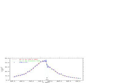
Figure 15: The new CMD-2 data on the pion form–factor versus Gounaris–Saurai like parametrizations.

For other parameterizations see e.g. Kuhn:1990ad ; Benayoun:1997ex . In fact the pion form factor can be “parametrized” in a more model independent way by exploiting analyticity, unitarity and constraints from chiral perturbation theory together with information from $\pi\pi$ scattering data and by combining $|F_{\pi}(s)|^{2}$ data in both the space–like and the time–like region Casas:1985yw ; Guerrero:1997ku ; Bijnens:1998fm ; Colangelo:2001df ; DeTroconiz:2001wt .

It is the aim to extract $F_{\pi}$ from experimental data by undressing the experimentally observed cross sections from radiative corrections. Using the usual procedure of unfolding the QED corrections leads to a model dependence for the results which can be estimated by a comparison of different form factor parameterizations. In our radiative return scenario we can get $|F_{\pi}(s)|^{2}$ directly via (55). Note that for this $|F_{\pi}(M_{\phi}^{2})|^{2}$ has to be determined at an accuracy of $10\,\%$ or better.

Why is the above form factor ansatz a reasonable one to parametrize the extended structure of the strongly interacting bound state pion? First of all it leads to the right long range behavior if $F_{\pi}(0)=1$ which corresponds to pure scalar QED. It also allows for a consistent treatment of radiative corrections under the condition that one should not think of a form factor as being related to a pion vertex but to the Born amplitude (factorization):

$${\cal M}_{0}(s)[e^{+}e^{-}\to\pi^{+}\pi^{-}] = {\cal M}_{0}^{point}(s)\times F_{\pi}(s)\;.$$ (74)

${\cal M}_{0}^{point}$ is the Born amplitude for point-like pions, obtained from scalar QED. For higher order virtual plus soft photon corrections the amplitudes can then be written as

$${\cal M}_{v+s}(s) = \delta_{v+s}\times{\cal M}_{0}^{point}(s)\times F_{\pi}(s)$$ (75)

$$+ \left(\mbox{terms}\to\frac{m_{e}^{2}}{s}\right)\;.$$

The factor $\delta_{v+s}$ is again calculated by scalar QED. Clearly this ansatz respects gauge invariance, the renormalization procedure of scalar QED can then be applied and the cancellation of infrared divergences is also achieved.

Note that the “terms$\to m_{e}^{2}/s$” stands for non–factorizing IFS interference corrections. The above form may be assumed to hold as an approximation also for the hard photon FS corrections. Without further investigations we cannot say what is the systematic error we make by utilizing this ansatz, however (see the discussion towards the end of Sec. 4).

References

• (1) N. Cabibbo and R. Gatto, Phys. Rev. D124 (1961) 1577.
• (2) F. Jegerlehner, Z. Phys. C32 (1986) 195.
• (3) S. Eidelman and F. Jegerlehner, Z. Phys. C67 (1995) 585, and references therein.
• (4) M. Gourdin and E. De Rafael, Nucl. Phys. B10 (1969) 667.
• (5) T. Kinoshita, B. Nižić and Y. Okamata, Phys. Rev. Lett. 52 (1984) 717; Phys. Rev. D31 (1985) 2108.
• (6) R. Alemany, M. Davier, A. Höcker, Eur. Phys. J. C2 (1998) 123.
• (7) M. Davier, A.  Höcker, Phys. Lett. B435 (1998) 427.
• (8) F. Jegerlehner, Hadronic effects in $(g-2)_{\mu}$ and $\alpha_{\rm QED}(M_{Z})$: Status and perspectives, in Radiative Corrections, ed. J. Solà, World Scientific, Singapore, 1999.
• (9) F. Jegerlehner, hep-ph/0104304.
• (10) S. Narison, hep-ph/0103199.
• (11) J. F. De Troconiz and F. J. Yndurain, hep-ph/0106025.
• (12) G. Cvetic, T.  Lee and I. Schmidt, hep-ph/0107069.
• (13) H. N. Brown et al. Phys. Rev. Lett. 86 (2001) 2227.
• (14) F. J. Yndurain, hep-ph/0102312.
• (15) K. Melnikov, hep-ph/0105267.
• (16) A. Czarnecki and W. J. Marciano, Phys. Rev. D64 (2000) 013014 [hep-ph/0102122].
• (17) M. Knecht and A. Nyffeler, hep-ph/0111058.
• (18) M. Knecht, A. Nyffeler, M. Perrottet and E. De Rafael, hep-ph/0111059.
• (19) M. Hayakawa and T. Kinoshita, hep-ph/0112102.
• (20) I. Blokland, A. Czarnecki and K. Melnikov, hep-ph/0112117.
• (21) J. Bijnens, E. Pallante and J. Prades, hep-ph/0112255.
• (22) H. Czyz and J. H. Kühn, Eur. Phys. J. C18 (2001) 497 [hep-ph/0008262].
• (23) G. Cataldi, A. Denig, W. Kluge, S. Müller, and G. Venanzoni, Measurement of the hadronic cross section with KLOE using a radiated photon in the initial state, in Frascati 1999, Physics and detectors for DAPHNE p. 569.
• (24) R. R. Akhmetshin et al. (CMD-2 Collaboration), Measurement of $e^{+}e^{-}\rightarrow\pi^{+}\pi^{-}$ cross-section with CMD-2 around $\rho$ meson, BUDKERINP-99-10, hep-ex/9904027; Recent Results from CMD-2 Detector at VEPP-2M, BUDKERINP-99-11, http://www.inp.nsk.su/publications.
• (25) R. R. Akhmetshin et al. [CMD-2 Collaboration], hep-ex/0112031.
• (26) S. Spagnolo, Eur. Phys. J. C6 (1999) 637.
• (27) A. B. Arbuzov, E. A. Kuraev, N. P. Merenkov and L. Trentadue, JHEP 12 (1998) 009 [hep-ph/9804430].
• (28) S. Binner, J. H. Kühn, and K. Melnikov, Phys. Lett. B459 (1999) 279 [hep-ph/9902399.]
• (29) M. I. Konchatnij and N. P. Merenkov, JETP Lett.  69 (1999) 811 [hep-ph/9903383].
• (30) V. A. Khoze et al., Eur. Phys. J. C18 (2001) 481 [hep-ph/0003313].
• (31) M. Benayoun, S. I. Eidelman, V. N. Ivanchenko and Z. K. Silagadze, Mod. Phys. Lett. A14 (1999) 2605 [hep-ph/9910523].
• (32) J. Z. Bai et al. [BES Collaboration], hep-ex/0102003;
G. S. Huang [representing the BES Collaboration], hep-ex/0105074.
• (33) F. A. Berends, W. L. van Neerven and G. J. Burgers, Nucl. Phys. B297 (1988) 429 [Erratum-ibid. B304 (1988) 921].
• (34) G. Montagna, O. Nicrosini, F. Piccinini, Phys. Lett. B406 (1997) 243.
• (35) B. A. Kniehl, M. Krawczyk, J. H. Kühn and R. G. Stuart, Phys. Lett. B209 (1988) 337.
• (36) A. B. Arbuzov, hep-ph/9907500.
• (37) M. Skrzypek, Acta Phys. Pol. B23 (1992) 135.
• (38) B. Kubis and U. G. Meissner, Nucl. Phys. A671 (2000) 332 [Erratum-ibid. A692 (2000) 647] [hep-ph/9908261].
• (39) G. Bonneau and F. Martin, Nucl. Phys. B27 (1971) 381; D.R. Yennie, Phys. Rev. Lett. 34 (1975) 239; J.D. Jackson and D.L. Scharre, Nucl. Instrum. Methods 128 (1975) 13; M. Greco, G. Pancheri-Srivastava and Y. Srivastava, Nucl. Phys. B101 (1975) 234; B202 (1980) 118.
• (40) Y.S. Tsai, SLAC-PUB-1515 (1975); SLAC-PUB-3129 (1983).
• (41) F.A. Berends et al., Nucl. Phys. B57 (1973) 381; Nucl. Phys. B68 (1974) 541; F.A. Berends and R. Kleiss, Nucl. Phys. B178 (1981) 141; F.A. Berends, R. Kleiss and S. Jadach, Nucl. Phys. B202 (1982) 63; F.A. Berends and R. Kleiss, Nucl. Phys. B228 (1983) 537.
• (42) S.I. Eidelman and E.A. Kuraev, Phys. Lett. B80 (1978) 94; V.N. Baier, V.S. Fadin, V.A. Khoze and E.A. Kuraev, Phys. Rep. C78 (1981) 293; E.A. Kuraev and V.S. Fadin, Sov. J. Nucl. Phys.  41 (1985) 466.
• (43) A. B. Arbuzov et al., JHEP 10 (1997) 006.
• (44) F. Bloch and A. Nordsieck, Phys. Rev. D52 (1937) 54.
• (45) D. R. Yennie, S. C. Frautschi, H. Suura, Ann. Phys. 13 (1961) 379.
• (46) T. Kinoshita, J. Math. Phys. 3 (1962) 650.
• (47) T. D. Lee and M. Nauenberg, Phys. Rev. D133 (1964) B1549.
• (48) J. S. Schwinger, Particles, Sources, And Fields. Vol. 3, Redwood City, USA: Addison-Wesley (1989) p. 99.
• (49) M. Drees and K. Hikasa, Phys. Lett. B252 (1990) 127.
• (50) A. Hoefer, Radiative Corrections to Hadron Production in $e^{+}e^{-}$ Annihilation at DAPHNE Energies, Doctor Thesis, Humboldt University at Berlin, October 2001.
• (51) S. Jadach, B. F. L. Ward, and Z. Was, Comput. Phys. Commun. 130 (2000) 260.
• (52) V. M. Budnev, I. F. Ginzburg, G. V. Meledin and V. G. Serbo, Phys. Rept.  15 (1974) 181.
• (53) H. Krasemann and J. A. Vermaseren, Nucl. Phys. B 184 (1981) 269.
• (54) I. F. Ginzburg, A. Schiller and V. G. Serbo, Eur. Phys. J. C 18 (2001) 731 [hep-ph/0012069].
• (55) G. Rodrigo, A. Gehrmann-De Ridder, M. Guilleaume and J. H. Kühn, hep-ph/0106132.
• (56) G. Rodrigo, H. Czyz, J. H. Kuhn and M. Szopa, hep-ph/0112184.
• (57) F. Jegerlehner, Nucl. Phys. Proc. Suppl. 51C (1996) 131 [hep-ph/9606484].
• (58) G. Källén and A. Sabry, K. Dan. Vidensk. Selsk. Mat.-Fys. Medd. 29 (1955) No. 17.
• (59) G. J. Gounaris, J. J Sakurai, Phys. Rev. Lett. 21 (1968) 244.
• (60) A. Quenzer et al., Phys. Lett. B76 (1978) 512.
• (61) T. Kinoshita, B. Nizic, and Y. Okamoto. Phys. Rev. D31 (1985) 2108.
• (62) J. H. Kühn, A. Santamaria, Z. Phys. C48 (1990) 445.
• (63) M. Benayoun et al., Eur. Phys. J. C2 (1998) 269.
• (64) J. A. Casas, C. Lopez and F. J. Yndurain, Phys. Rev. D32 (1985) 736.
• (65) F. Guerrero and A. Pich, Phys. Lett. B412 (1997) 382 [hep-ph/9707347].
• (66) J. Bijnens, G. Colangelo and P. Talavera, JHEP 9805 (1998) 014 [hep-ph/9805389].
• (67) G. Colangelo, J. Gasser and H. Leutwyler, Nucl. Phys. B603 (2001) 125 [hep-ph/0103088].