DESY 01-101
Recent Progress in Leptogenesis

Abstract

After recalling the general virtues of leptogenesis we compare two realizations, Affleck-Dine leptogenesis and thermal leptogenesis, which generically lead to different predictions for neutrino masses. Finally, we describe the progress towards a full quantum mechanical description of the basic non-equilibrium process of leptogenesis beyond the approximations involved in Boltzmann’s equations.

1 Why Leptogenesis ?

One of the main successes of the standard early-universe cosmology is the prediction of the abundances of the light elements, D, ³He, ⁴He and ⁷Li. Agreement between theory and observation is obtained for a certain range of the parameter $\eta$, the ratio of baryon density and photon density[1],

$$\eta={n_{B}\over n_{\gamma}}=(1.5-6.3)\times 10^{-10}\;,$$ (1)

where the present number density of photons is $n_{\gamma}\sim 400/{\rm cm}^{3}$. Since no significant amount of antimatter is observed in the universe, the baryon density yields directly the cosmological baryon asymmetry, $Y_{B}=(n_{B}-n_{\bar{B}})/s\simeq\eta/7$, where $s$ is the entropy density.

A matter-antimatter asymmetry can be dynamically generated in an expanding universe if the particle interactions and the cosmological evolution satisfy Sakharov’s conditions[2],i.e.,

• baryon number violation

• $C$ and $C\!P$ violation

• deviation from thermal equilibrium .

Although the baryon asymmetry is just a single number, it provides an important relationship between the standard model of cosmology, i.e., the expanding universe with Robertson-Walker metric, and the standard model of particle physics as well as its extensions.

At present there exist a number of viable scenarios for baryogenesis. They can be classified according to the different ways in which Sakharov’s conditions are realized. Already in the standard model $C$ and $C\!P$ are not conserved. Also baryon number ($B$) and lepton number ($L$) are violated by instanton processes[3]. In grand unified theories $B$ and $L$ are broken by the interactions of gauge bosons and leptoquarks. This is the basis of the classical GUT baryogenesis[4]. Analogously, the $L$-violating decays of heavy Majorana neutrinos lead to leptogenesis[5]. The initial abundance of the heavy neutrinos may be generated either thermally or from inflaton decays[6, 7]. In supersymmetric theories the existence of approximately flat directions in the scalar potential allows for new possibilities. Coherent oscillations of scalar fields may then generate large asymmetries[8].

The crucial departure from thermal equilibrium can also be realized in several ways. One possibility is a sufficiently strong first-order electroweak phase transition[9]. In this case $C\!P$ violating interactions of the standard model or its supersymmetric extension could in principle generate the observed baryon asymmetry. However, due to the rather large lower bound on the Higgs boson mass of about 115 GeV, which is imposed by the LEP experiments, this interesting possibility is now restricted to a very small range of parameters in the supersymmetric standard model. In the case of the Affleck-Dine scenario the baryon asymmetry is generated at the end of an inflationary period as a coherent effect of scalar fields which leads to an asymmetry between quarks and antiquarks after reheating[10]. For the classical GUT baryogenesis and for leptogenesis the departure from thermal equilibrium is due to the deviation of the number density of the decaying heavy particles from the equilibrium number density. How strong this deviation from thermal equilibrium is depends on the lifetime of the decaying heavy particles and the cosmological evolution. Further scenarios for baryogenesis are described in ref.[11].

The theory of baryogenesis involves non-perturbative aspects of quantum field theory and also non-equilibrium statistical field theory, in particular the theory of phase transitions and kinetic theory.

Figure 1: One of the 12-fermion processes which are in thermal equilibrium in the high-temperature phase of the standard model.

A crucial ingredient is the connection between baryon number and lepton number in the high-temperature, symmetric phase of the standard model. Due to the chiral nature of the weak interactions $B$ and $L$ are not conserved. At zero temperature this has no observable effect due to the smallness of the weak coupling. However, as the temperature approaches the critical temperature $T_{EW}$ of the electroweak transition, $B$ and $L$ violating processes come into thermal equilibrium[12].

The rate of these processes is related to the free energy of sphaleron-type field configurations which carry topological charge. In the standard model they lead to an effective

Figure 2: Sphaleron rate in Bödeker’s effective theory, two lattice implementations of the HTL effective theory, and pure lattice theory interpreted as HTL effective theory[14].

interaction of all left-handed quarks and leptons[3] (cf. fig. 1),

$$O_{B+L}=\prod_{i}\left(q_{Li}q_{Li}q_{Li}l_{Li}\right)\;,$$ (2)

which violates baryon and lepton number by three units,

$$\Delta B=\Delta L=3\;.$$ (3)

The evaluation of the sphaleron rate in the symmetric high-temperature phase is a complicated problem. A clear physical picture has been obtained in Bödeker’s effective theory[13] according to which low-frequency gauge field fluctuations satisfy the equation of motion

$${\bf D}\times{\bf B}=\sigma{\bf E}-{\bf\zeta}\;.$$ (4)

Here $\bf\zeta$ is Gaussian noise, i.e., a random vector field with variance

$$\langle\zeta_{i}(t,{\bf x})\zeta_{j}(t^{\prime},{\bf x^{\prime}})\rangle=2\sigma\delta_{ij}\delta(t-t^{\prime})\delta({\bf x}-{\bf x^{\prime}})\;,$$ (5)

and $\sigma$ is a non-abelian conductivity. The sphaleron rate can then be written as[14],

$$\Gamma\simeq(14.0\pm 0.3){1\over\sigma}(\alpha_{w}T)^{5}\;.$$ (6)

A comparison with two lattice simulations is shown in fig. 2. From this one derives that $B$- and $L$-violating processes are in thermal equilibrium for temperatures in the range

$$T_{EW}\sim 100\ \mbox{GeV}<T<T_{SPH}\sim 10^{12}\ \mbox{GeV}\;.$$ (7)

Sphaleron processes have a profound effect on the generation of the cosmological baryon asymmetry, in particular in connection with the dominant lepton number violating interactions between lepton and Higgs fields,

$${\cal L}_{\Delta L=2}={1\over 2}f_{ij}\ l^{T}_{Li}\phi Cl_{Lj}\phi+\mbox{ h.c.}\;.$$ (8)

Such an interaction arises in particular from the exchange of heavy Majorana neutrinos. In the Higgs phase of the standard model, where the Higgs field acquires a vacuum expectation value, it gives rise to Majorana masses of the light neutrinos $\nu_{e}$, $\nu_{\mu}$ and $\nu_{\tau}$.

One may be tempted to conclude from eq. (3) that any $B+L$ asymmetry generated before the electroweak phase transition, i.e., at temperatures $T>T_{EW}$, will be washed out. However, since only left-handed fields couple to sphalerons, a non-zero value of $B+L$ can persist in the high-temperature, symmetric phase in case of a non-vanishing $B-L$ asymmetry. An analysis of the chemical potentials of all particle species in the high-temperature phase yields a relation between the baryon asymmetry $Y_{B}=(n_{B}-n_{\bar{B}})/s$ and the corresponding $B-L$ and $L$ asymmetries $Y_{B-L}$ and $Y_{L}$, respectively[15],

$$Y_{B}\ =\ a\ Y_{B-L}\ =\ {a\over a-1}\ Y_{L}\;.$$ (9)

The number $a$ depends on the other processes which are in thermal equilibrium. If these are all standard model interactions one has $a=28/79$. If instead of the Yukawa interactions of the right-handed electron the $\Delta L=2$ interactions (8) are in equilibrium one finds $a=-2/3$  [16].

From eq. (9) one concludes that the cosmological baryon asymmetry, if generated before the electroweak transition, requires also a lepton asymmetry, and therefore lepton number violation. This leads to an intriguing interplay between Majorana neutrinos masses, which are generated by the lepton-Higgs interactions (8), and the baryon asymmetry: lepton number violating interactions are needed in order to generate a baryon asymmetry; however, they have to be sufficiently weak, so that they fall out of thermal equilibrium at the right time and a generated asymmetry can survive until today.

The connection between baryon and lepton number at high temperatures leads to very attractive new mechanisms to generate the cosmological baryon asymmetry. This includes large lepton number violating classical fields generated during an inflationary phase and the out-of-equilibrium decays of heavy Majorana neutrinos. In the following we shall compare these two versions of leptogenesis which generically make different predictions for neutrino masses.

2 Affleck-Dine leptogenesis

In supersymmetric theories the $\Delta L=2$ lepton-Higgs interactions (8) are contained in the superpotential

$$W={1\over 2M_{i}}\phi L_{i}\phi L_{i}\;,$$ (10)

where $H_{2}$ and $L_{i}$, $i=1\ldots 3$ denote Higgs and lepton superfields in a particular basis, respectively. The supersymmetric standard model possesses the D-flat direction[17]

$$\phi=\left(\begin{array}[]{c}\varphi\\ 0\end{array}\right)\;,\quad L_{1}=\left(\begin{array}[]{c}0\\ \varphi\end{array}\right)\;,$$ (15)

whose flatness is lifted by the non-renormalizable interaction (10) and by by various supergravity and finite-temperature corrections. Recently, leptogenesis based on this flat direction has been studied in detail[18, 19]. The complete scalar potential during an inflationary phase with Hubble parameter $H_{I}$ is given by[19]

$$V(\varphi,T) = \mu(T)^{2}|\varphi|^{2}+a_{g}\alpha_{s}^{2}T^{4}\ln{{|\varphi|^{2}\over T^{2}}}+{m_{3/2}\over 8M_{1}}\left(a_{m}\varphi^{4}+c.c.\right)+{1\over 4M^{2}}|\varphi|^{6}$$ (16)

$$-c_{I}H_{I}^{2}|\varphi|^{2}+{H_{I}\over 8M_{1}}\left(a_{H}\varphi^{4}+c.c.\right)\;.$$

Here $a_{g}={\cal O}(1)$ is a parameter which depends on the particle content of the theory, $m_{3/2}a_{m}$ reflects supersymmetry breaking at $T=0$, whereas $c_{I}H_{I}^{2}$ and $H_{I}a_{H}$ are due to the breaking of supersymmetry during inflation. Note, that the coefficient $c_{I}$ has to be positive for Affleck-Dine leptogenesis to work whereas the simplest canonical Kähler potential would yield the opposite sign for $c_{I}$!

Figure 3: Contour plot for the baryon asymmetry $Y_{B}=n_{B}/s$ in the $m_{\nu_{1}}\mbox{[eV]}(horizontal)-T_{R}\mbox{[GeV]}$(vertical)-plane. The full lines correspond to $Y_{B}=10^{-9}$, $10^{-10}$, $10^{-11}$ and $10^{-12}$ from left to right. The short-dashed lines represent the results obtained negleting thermal effects; the long-dashed lines give the baryon asymmetries if only thermal masses are included. The shaded region corresponds to the observed baryon asymmetry[19].

The assumed phase difference between the complex numbers $a_{m}$ and $a_{H}$ is responsible for the generation of a lepton asymmetry. During the inflationary phase the field $\varphi$ is driven to one of the discrete minima

$$|\varphi|=\varphi_{0}\sim(MH_{I})^{1/2}\;,\quad arg(\varphi)={1\over 4}(-arg(a_{H})+(2n+1)\pi)\;,\;n=0\ldots 3\;.$$ (17)

After inflation, when $\mu(T)^{2}$ starts to be the dominant mass term, the homogeneous field $\varphi$ begins coherent oscillations which eventually lead to an asymmetry in the number densities for ordinary leptons and scalar leptons and, finally, via the sphaleron processes to an asymmetry in baryon number. It is remarkable that the final baryon asymmetry is rather insensitive to the reheating temperature after inflation in the range $T_{R}\simeq 10^{5}\ldots 10^{12}$GeV. A detailed calculation yields[19],

$${n_{B}\over s}\simeq 10^{-11}\delta_{eff}\left({m_{\nu_{1}}\over 10^{-8}\mbox{eV}}\right)^{-3/2}\left({m_{3/2}|a_{m}|\over 1\mbox{TeV}}\right)\;,$$ (18)

i.e., the baryon asymmetry is determined by the lightest neutrino mass and the strength of supersymmetry breaking. For an effective $C\!P$-violating angle $\delta_{eff}\simeq 0.1\ldots 1$ and $m_{3/2}|a_{m}|\simeq 1$TeV, the observed baryon asymmetry is obtained for an ‘ultralight’ neutrino,

$$m_{\nu_{1}}\simeq(0.1-1)\times 10^{-9}\mbox{eV}\;.$$ (19)

This small neutrino mass reflects the required flatness of the D-flat direction for successful Affleck-Dine leptogenesis.

Figure 4: $m_{\nu e\nu e}$[eV] as function of $\sin^{2}{\theta_{sol}}\sqrt{\Delta m^{2}_{sol}}$[eV] for the large angle MSW solution and $|U_{e3}|<0.10$[19].

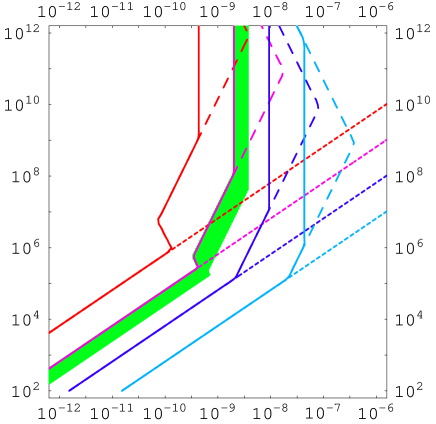
The prediction of an ultralight neutrino has direct implications for neutrinoless double beta decay. The effective neutrino mass which determines the decay rate is given by $m_{\nu_{e}\nu_{e}}=|\sum_{i}U_{ei}^{2}m_{\nu_{i}}|$, where $m_{\nu_{i}}$ are the neutrino masses and $U_{\alpha i}$ the neutrino mixing matrix, respectively. For hierarchical neutrinos with an ultralight lowest state $m_{\nu_{e}\nu_{e}}$ can be expressed in terms of the oscillation parameters determined from the solar and the atmospheric neutrino deficits,

$$m_{\nu_{e}\nu_{e}}=\left|\left(1-|U_{e3}|^{2}\right)\sin^{2}{\theta_{sol}}\sqrt{\Delta m^{2}_{sol}}+|U_{e3}|^{2}e^{i\alpha}\sqrt{\Delta m^{2}_{atm}}\right|\;.$$ (20)

It is remarkable that for the large angle MSW solution $m_{\nu_{e}\nu_{e}}$ reaches the value of $m_{\nu_{2}}\simeq\sqrt{\Delta m^{2}_{sol}}\simeq 3\times 10^{-3}-10^{-2}$[eV] (cf. fig. 4), which may be accessible in future neutrinoless double beta decay experiments.

3 Thermal Leptogenesis

Here one starts from a thermal distribution of heavy Majorana fermions which have $C\!P$ violating decay modes into standard model leptons. The natural candidates are the three right-handed neutrinos $\nu_{Ri}$, $i=1\ldots 3$, whose interactions are described by the lagrangian,

$${\cal L}=\overline{l}_{L}\phi^{*}\lambda^{*}\nu_{R}-{1\over 2}\overline{\nu}_{R}^{c}M\nu_{R}+h.c.$$ (21)

$M$ is a Majorana mass matrix. The vacuum expectation value of the Higgs field $\left\langle\phi\right\rangle=v$ generates the Dirac mass term $m_{D}=h_{\nu}v$ which is assumed to be small compared to the Majorana mass $M$. This yields light and heavy neutrino mass eigenstates according to the seesaw mechanism[20],

$$\nu\simeq V_{\nu}^{T}\nu_{L}+\nu_{L}^{c}V_{\nu}^{*}\quad,\qquad N\simeq\nu_{R}+\nu_{R}^{c}\,,$$ (22)

with masses

$$m_{\nu}\simeq-V_{\nu}^{T}m_{D}^{T}{1\over M}m_{D}V_{\nu}\,\quad,\quad m_{N}\simeq M\;,$$ (23)

where $V_{\nu}$ is the neutrino mixing matrix.

We shall restrict our discussion to the case of hierarchical Majorana neutrino masses, $M_{1}\ll M_{2},M_{3}$. The baryon asymmetry is then determined by the $C\!P$ violating decays of the lightest Majorana neutrino $N_{1}=\nu_{R1}+\nu_{R1}^{c}\equiv N$,

$$\Gamma(N\rightarrow l\phi)={1\over 2}(1+\varepsilon)\Gamma\;,\quad\Gamma(N\rightarrow\bar{l}\bar{\phi})={1\over 2}(1-\varepsilon)\Gamma\;.$$ (24)

Here $\Gamma=(\lambda^{\dagger}\lambda)_{11}M/(8\pi)$ is the total decay width, and the parameter $\varepsilon\ll 1$ measures the amount of $C\!P$ violation. The generation of the baryon asymmetry takes place at a temperature $T\sim M=M_{1}\ll M_{2},M_{3}$. It is therefore convenient to describe the system by an effective lagrangian where the two heavier neutrinos have been integrated out,

$${\cal L} = \overline{l}_{Li}\phi^{*}\lambda^{*}_{i1}N+N^{T}\lambda_{i1}Cl_{Li}\phi-{1\over 2}MN^{T}CN$$ (25)

$$+{1\over 2}\eta_{ij}l_{Li}^{T}\phi Cl_{Lj}\phi+{1\over 2}\eta^{*}_{ij}\overline{l}_{Li}\phi^{*}C\overline{l}_{Lj}^{T}\phi^{*}\;,$$

with

$$\eta_{ij}=\sum_{k=2}^{3}\lambda_{ik}{1\over M_{k}}\lambda^{T}_{kj}\;.$$ (26)

The $C\!P$ asymmetry $\varepsilon$ arises from one-loop vertex and self-energy corrections[21, 22, 23]. It can be expressed in a compact form as[24]

$$\varepsilon={3\over 16\pi}{\mbox{Im}(\lambda^{\dagger}\eta\lambda^{*})_{11}\over(\lambda^{\dagger}\lambda)_{11}}M\;.$$ (27)

Given the Dirac and Majorana neutrino mass matrices the $C\!P$ asymmetry $\varepsilon$ and, consequently, the baryon asymmetry are determined. Consider as an example a pattern of fermion masses based on the group $SU(5)_{GUT}\times U(1)_{F}$, where $U(1)_{F}$ is a spontaneously broken generation symmetry. The Yukawa couplings arise from non-renormalizable interactions with a gauge singlet field $\Phi$ which acquires a vacuum expectation value[25],

$$\lambda_{ij}=g_{ij}\left({\left\langle\Phi\right\rangle\over\Lambda}\right)^{Q_{i}+Q_{j}}\;.$$ (28)

Here $g_{ij}$ are couplings ${\cal O}(1)$ and $Q_{i}$ are the $U(1)_{F}$ charges of the various fermions, with $Q_{\Phi}=-1$. The interaction scale $\Lambda$ is usually chosen to be very large, $\Lambda>\Lambda_{GUT}$. An example of possible charges $Q_{i}$ is given in table 1.

Table 1: Chiral charges of charged and neutral leptons with $SU(5)_{GUT}\times U(1)_{F}$ symmetry.

$\psi_{i}$	$e^{c}_{R3}$	$e^{c}_{R2}$	$e^{c}_{R1}$	$l_{L3}$	$l_{L2}$	$l_{L1}$	$\nu^{c}_{R3}$	$\nu^{c}_{R2}$	$\nu^{c}_{R1}$
$Q_{i}$	0	1	2	$0$	$0$	$1$	0	$1$	$2$

The assignment of the same charge to the lepton doublets of the second and third generation leads to a neutrino mass matrix of the form[26, 27],

$$m_{\nu_{ij}}\sim\left(\begin{array}[]{ccc}\epsilon^{2}&\epsilon&\epsilon\\ \epsilon&\;1&1\\ \epsilon&1&1\end{array}\right){v_{2}^{2}\over\left\langle R\right\rangle}\;.$$ (29)

This structure immediately yields a large $\nu_{\mu}-\nu_{\tau}$ mixing angle. The phenomenology of neutrino oscillations depends on the unspecified coefficients which are ${\cal O}(1)$. The flavour mixing parameter $\epsilon$ is chosen to be $\left\langle\Phi\right\rangle/\Lambda=\epsilon\sim 1/17$, which corresponds to the mass ratio $m_{\mu}/m_{\tau}$.

One easily verifies that the mass ratios of heavy and light Majorana neutrinos are given by

$$M_{1}:M_{2}:M_{3}\sim\epsilon^{4}:\epsilon^{2}:1\;,\quad m_{1}:m_{2}:m_{3}\sim\epsilon^{2}:1:1\;.$$ (30)

The masses of the two eigenstates $\nu_{2}$ and $\nu_{3}$ depend on the unspecified factors ${{\cal O}(1)}$. They are therefore consistent with the mass differences $\Delta m^{2}_{\nu_{1}\nu_{2}}\simeq 10^{-5}-10^{-3}$ eV² inferred from the large angle MSW solution of the solar neutrino problem and $\Delta m^{2}_{\nu_{2}\nu_{3}}\simeq 10^{-3}-10^{-2}$ eV² associated with the atmospheric neutrino deficit[1]. In the following we we shall use for numerical estimates the geometric mean of the neutrino masses of the second and third family, $\overline{m}_{\nu}=(m_{\nu_{2}}m_{\nu_{3}})^{1/2}\sim 10^{-2}$ eV. The choice of the charges in table 1 corresponds to large Yukawa couplings of the third generation. For the mass of the heaviest Majorana neutrino one then finds

$$M_{3}\ \sim\ {v^{2}\over\overline{m}_{\nu}}\ \sim\ 10^{15}\ \mbox{GeV}\;,$$ (31)

which implies that $B-L$ is broken at the unification scale $\Lambda_{GUT}$.

The $C\!P$ asymmetry $\varepsilon$ (27) leads to a lepton asymmetry in the course of the cosmological evolution[28],

$$Y_{L}\ =\ {n_{L}-n_{\overline{L}}\over s}\ =\ \kappa\ {\varepsilon\over g_{*}}\;.$$ (32)

Here the factor $\kappa<1$ represents the effect of washout processes. In order to determine $\kappa$ one has to solve the full Boltzmann equations[29, 30]. Important processes are the $\Delta L=2$ lepton Higgs scatterings mediated by heavy neutrinos since cancellations between on-shell contributions to these scatterings and contributions from neutrino decays and inverse decays ensure that no asymmetry is generated in thermal equilibrium. Further, due to the large top-quark Yukawa coupling one has to take into account neutrino top-quark scatterings mediated by Higgs bosons[29, 30].

Figure 5: Time evolution of the heavy neutrino number density and the lepton asymmetry for the $SU(5)_{GUT}\times U(1)_{F}$ model. The solid line shows the solution of the Boltzmann equation for the right-handed neutrinos, while the corresponding equilibrium distribution is represented by the dashed line. The absolute value of the lepton asymmetry $Y_{L}$ is given by the dotted line and the hatched area shows the lepton asymmetry corresponding to the observed baryon asymmetry [16].

These processes are of crucial importance for leptogenesis, since they can create a thermal population of heavy neutrinos at high temperatures $T>M$.

In order to obtain the baryon asymmetry predicted by the model of neutrino masses described above we first have to evaluate the $C\!P$ asymmmetry. Since for the Yukawa couplings only the powers in $\epsilon$ are known, we will also obtain the $C\!P$ asymmetry and the corresponding baryon asymmetry to leading order in $\epsilon$, i.e., up to unknown factors ${\cal O}(1)$. Note, that for models with a $U(1)_{F}$ generation symmetry the baryon asymmetry is ‘quantized’, i.e., changing the $U(1)_{F}$ charges will change the baryon asymmetry by powers of $\epsilon$[31]. One easily obtains from eqs. (27), (28) and the table[31],

$$\varepsilon\ \sim\ {3\over 16\pi}\ \epsilon^{4}\;.$$ (33)

Using $\epsilon^{2}\sim 1/300$ and $g_{*}\sim 100$ one then obtains the baryon asymmetry,

$$Y_{B}\sim\kappa\ 10^{-8}\;.$$ (34)

For $\kappa\sim 0.1\ldots 0.01$ this is indeed the correct order of magnitude! The baryogenesis temperature is given by the mass of the lightest of the heavy Majorana neutrinos,

$$T_{B}\sim M_{1}\sim\epsilon^{4}M_{3}\sim 10^{10}\ \mbox{GeV}\;.$$ (35)

For this model, where the $C\!P$ asymmetry is determined by the mass hierarchy of light and heavy Majorana neutrinos, baryogenesis has been studied in detail in ref[32]. It is remarkable that the observed baryon asymmety is obtained without any fine tuning of parameters, if $B-L$ is broken at the unification scale $\Lambda_{GUT}$. The generated baryon asymmetry does not depend on the flavour mixing of the light neutrinos, in particular the $\nu_{\mu}-\nu_{\tau}$ mixing angle.

The solution of the full Boltzmann equations is shown in fig. 5. The initial condition at a temperature $T\sim 10M_{1}$ is chosen to be a state without heavy neutrinos. The Yukawa interactions are sufficient to bring the heavy neutrinos into thermal equilibrium. At temperatures $T\sim M_{1}$ the familiar out-of-equilibrium decays set in, which leads to a non-vanishing baryon asymmetry. The final asymmetry agrees with the estimate (34) for $\kappa\sim 0.1$. The dip in fig. 5 is due to a change of sign in the lepton asymmetry at $T\sim M_{1}$.

The final baryon asymmetry is usually obtained from the final lepton asymmetry by means of eq. (9). Note, that this is conceptually not correct! The sphaleron processes are in equilibrium whereas the heavy neutrino decays out of equilibrium. Hence, any generated asymmetry is immediately distributed among other degrees of freedom in the plasma. This effect reduces the generated baryon asymmetry by a factor ${{\cal O}(1)}$[33].

4 Towards the Theory of Leptogenesis

The generation of a baryon asymmetry is an out-of-equilibrium process which is generally treated by means of Boltzmann equations. A shortcoming of this approach is that the Boltzmann equations are classical equations for the time evolution of phase space distribution functions. On the contrary, the involved collision terms are $S$-matrix elements which involve quantum interferences of different amplitudes in a crucial manner. Clearly, a full quantum mechanical treatment is highly desirable. This is also required in order to justify the use of the Boltzmann equations and to determine the size of corrections.

All information about the time evolution of a system is contained in the time dependence of its Green functions[34, 35] which can be determined by means of Dyson-Schwinger equations. Originally these techniques were developed for non-relativistic many-body problems. More recently, they have also been applied to transport phenomena in nuclear matter[36], the electroweak plasma[37, 38] and the QCD plasma[39]. Alternatively, one may study the time evolution of density matrices[40, 41]. In the following we shall describe how the Green function technique can be used to obtain a systematic perturbative expansion around a solution of the Boltzmann equations[24].

The time evolution of an arbitrary multi-particle lepton-Higgs system can be studied by means of the Green functions of lepton and Higgs fields. For the heavy Majorana neutrino one has

$$iG_{\alpha\beta}(x_{1},x_{2})=\mbox{Tr}\left(\rho\hat{T}N_{\alpha}(x_{1})N_{\beta}(x_{2})\right)\;,$$ (36)

where $\hat{T}$ denotes the time ordering, $\rho$ is the density matrix of the system, the trace extends over all states, and the time coordinates $t_{1}$ and $t_{2}$ lie on an appropriately chosen contour $C$ in the complex plane[42]. $G(x_{1},x_{2})$ can be written as a sum of two parts,

$$G(x_{1},x_{2})=\Theta(t_{1}-t_{2})G^{>}(x_{1},x_{2})+\Theta(t_{2}-t_{1})G^{<}(x_{1},x_{2})\;.$$ (37)

For a system in thermal equilibrium at a temperature $T=1/\beta$ the density matrix is $\rho=\exp{(-\beta H)}$, where $H$ is the Hamilton operator. In this case the Green function only depends on the difference of coordinates and it is convenient to work with the Fourier transform $G(p)$. The contour $C$ can be chosen as a sum of two branches, $C=C_{1}\cup C_{2}$, which lie above and below the real axis. The time coordinates are real and associated with one of the two branches. Correspondingly, the Green function becomes a $2\times 2$ matrix,

$$G(p)=\left(\begin{array}[]{cc}G^{11}(p)&G^{12}(p)\\[4.30554pt] G^{21}(p)&G^{22}(p)\end{array}\right)\;.$$ (40)

The off-diagonal terms are given by

$$G^{12}(p)=G^{<}(p)\;,\quad G^{21}(p)=G^{>}(p)\;,$$ (41)

the diagonal terms of the matrix (40) are the familiar causal and anti-causal Green functions. The free Green functions are explicitly given by

$$iG^{>}(p) = \left(\Theta(p_{0})-\Theta(p_{0})f_{N}(E)-\Theta(-p_{0})f_{\bar{N}}(E)\right)\rho_{N}(p)\;,$$ (42)

$$iG^{<}(p) = \left(\Theta(-p_{0})-\Theta(p_{0})f_{N}(E)-\Theta(-p_{0})f_{\bar{N}}(E)\right)\rho_{N}(p)\;,$$ (43)

with the spectral density

$$\rho_{N}(p)=2\pi(\hbox to0.0pt{\hbox{$\mskip 1.0mu/$}\hss}p+M)C^{-1}\delta(p^{2}-M^{2})\;,$$ (44)

and the Fermi-Dirac distribution functions

$$f_{N}(E)=f_{\bar{N}}(E)={1\over e^{\beta E}+1}\ ,\quad E=\sqrt{M^{2}+p^{2}}\;.$$ (45)

Since $N(x)$ is a Majorana field one has $f_{N}=f_{\bar{N}}$, and the charge conjugation matrix $C$ occurs in the spectral density (44). The Green functions $S(x_{1},x_{2})$ and $\Delta(x_{1},x_{2})$ for the lepton doublets and the Higgs doublet also depend on chemical potentials. The Schwinger-Dyson equations for the Green functions $G^{>}(x_{1},x_{2})$, $G^{<}(x_{1},x_{2})$, etc. are usually referred to as Kadanoff-Baym equations.

For processes where the overall time evolution is slow compared to relative motions the Kadanoff-Baym equations can be solved in a derivative expansion. One considers the Wigner transform for $G(x_{1},x_{2})$,

$$G(x,p)=\int d^{4}y\ e^{ipy}\ G\left(x+{y\over 2},x-{y\over 2}\right)\;,$$ (46)

and for $S(x,p)$ and $\Delta(x,p)$, respectively. To leading order in the derivative expansion the Kadanoff-Baym equations become local in the space-time coordinate $x$. Keeping to zeroth order only the on-shell part of retarded and advanced Green functions and self-energies one obtains the equations

$$C({i\over 2}\hbox to0.0pt{\hbox{$\mskip 1.0mu/$}\hss}\partial+\hbox to0.0pt{\hbox{$\mskip 1.0mu/$}\hss}p-M)G^{>}(x,p) = C({i\over 2}\hbox to0.0pt{\hbox{$\mskip 1.0mu/$}\hss}\partial+\hbox to0.0pt{\hbox{$\mskip 1.0mu/$}\hss}p-M)G^{<}(x,p)$$ (47)

$$= {1\over 2}\left(\Sigma^{>}(x,p)G^{<}(x,p)-\Sigma^{<}(x,p)G^{>}(x,p)\right)\;,$$

$$({i\over 2}\hbox to0.0pt{\hbox{$\mskip 1.0mu/$}\hss}\partial+\hbox to0.0pt{\hbox{$\mskip 1.0mu/$}\hss}k)S^{>}(x,p) = ({i\over 2}\hbox to0.0pt{\hbox{$\mskip 1.0mu/$}\hss}\partial+\hbox to0.0pt{\hbox{$\mskip 1.0mu/$}\hss}k)S^{<}(x,p)$$ (48)

$$= {1\over 2}\left(\Pi^{>}(x,k)S^{<}(x,k)-\Pi^{<}(x,p)S^{>}(x,p)\right)\;.$$

The corresponding self-energies are shown in fig. (6).

Figure 6: One- and two-loop self energies for the lepton doublet.

Solutions of these equations yield the first terms for the non-equilibrium Green functions $G^{>}(x,p)$…$S^{<}(x,k)$ in an expansion involving off-shell effects and space-time variations which include ‘memory effects’.

Given the lepton self-energies we can now look for solutions of the equations (47) and (48). A straightforward calculation shows that the right-hand side of these equations vanishes for equilibrium Green functions and self-energies. Since leptogenesis is a process close to thermal equilibrium the solutions should be linear in the deviations,

$$\delta G(t,p) = G^{>}(t,p)-G^{>}_{eq}(p)=G^{<}(t,p)-G^{<}_{eq}(p)\;,$$ (49)

$$\delta S(t,p) = S^{>}(t,p)-S^{>}_{eq}(p)=S^{<}(t,p)-S^{<}_{eq}(p)\;.$$ (50)

One may also expect that $\delta G(t,p)$ and $\delta S(t,p)$ can be obtained from the equilibrium Green functions by a small change of the distribution functions,

$$i\delta G(x,p)=-\delta f_{N}(x,p)\rho_{N}(p)\;,\quad i\delta S(x,k)=-\epsilon(k_{0})\delta f_{l}(x,k)\rho_{l}(k)\;.$$ (51)

This ansatz indeed reduces the matrix equations (47) and (48) to the system of ordinary differential equations

$$E{\partial\over\partial{t}}\delta f_{N}(t,p) = -E{\partial\over\partial{t}}f_{N}(p)-2(\lambda^{\dagger}\lambda)_{11}\int d\Phi_{\bar{1}\bar{2}}(p)\delta f_{N}(t,p)p\cdot p_{1}\;,$$ (52)

$$g_{l}k{\partial\over\partial{t}}\delta f_{l}(t,k) = {3\over 8\pi}\mbox{Im}(\lambda^{\dagger}\eta\lambda^{*})_{11}M\int d\Phi_{\bar{1}2}(k)\delta f_{N}(t,p_{1})k\cdot p_{1}\$$ (53)

$$-2(\lambda^{\dagger}\lambda)_{11}\int d\Phi_{1\bar{2}}(k)\left(\delta f_{l}(t,k)f_{\phi}(p_{1})+f_{l}(k)\delta f_{\phi}(t,p_{1})\right)k\cdot p_{2}$$

$$-6{(\lambda^{\dagger}\lambda)^{2}_{11}\over M^{2}}\int d\Phi_{1\bar{2}\bar{3}}(k)\Big{(}2(\delta f_{l}(t,k)f_{\phi}(p_{1})+f_{l}(k)\delta f_{\phi}(t,p_{1})$$

$$\hskip 56.9055pt+\delta f_{l}(t,p_{2})f_{\phi}(p_{3})+f_{l}(p_{2})\delta f_{\phi}(t,p_{3}))k\cdot p_{2}$$

$$\hskip 56.9055pt+(\delta f_{l}(t,k)f_{l}(p_{1})+f_{l}(k)\delta f_{l}(t,p_{1})$$

$$\hskip 71.13188pt+2\delta f_{\phi}(t,p_{2})f_{\phi}(p_{3}))k\cdot p_{1}\Big{)}\ .$$

Here $g_{l}=6$ is the number of ‘internal’ degrees of freedom for three generations of lepton doublets, $d\Phi_{\bar{1}\bar{2}}(p)$ etc. denote phase space integrations, and $f_{N}(p)$, $f_{l}(p)$ and $f_{\phi}(p)$ are the equilibrium distributions of heavy neutrinos, lepton doublets and Higgs doublet, respectively.

Eqs. (52) and (53) are the Boltzmann equations for the distributions functions of heavy neutrinos and lepton doublets with the correct matrix elements for decays, $2\rightarrow 2$ processes and $C\!P$ violation. The effect of the Hubble expansion is included by means of the substitution $\partial/\partial t\rightarrow\partial/\partial t-Hp\partial/\partial p$. Integration over momenta then yields the more familiar form of the Boltzmann equations for the number densities. Note, that also the equilibrium distributions are time dependent since the temperature varies with time. The first term in eq. (53) drives the generation of a lepton asymmetry; the remaining terms tend to wash out an existing asymmetry.

We conclude that a solution of the Boltzmann equations generates a solution of the Kadanoff-Baym equations to leading order in the expansion described above. Various corrections such as relativistiv effects, ‘memory effects’, off-shell effects and deviations from kinetic equilibrium can now be systematically studied. By means of such an analysis one can obtain quantitative constraints on the parameters $M$, $(\lambda^{\dagger}\lambda)_{11}$ and $\varepsilon$, which relate the cosmological baryon asymmetry and neutrino properties.

5 Outlook

Detailed studies of the thermodynamics of the electroweak interactions at high temperatures have shown that in the standard model and most of its extensions the electroweak transition is too weak to affect the cosmological baryon asymmetry. Hence, one has to search for baryogenesis mechanisms above the Fermi scale.

Due to sphaleron processes baryon number and lepton number are related in the high-temperature symmetric phase of the standard model. As a consequence, the cosmological baryon asymmetry is related to neutrino properties. Generically, baryogenesis requires lepton number violation, which occurs in extensions of the standard model with right-handed neutrinos and Majorana neutrino masses. In detail the relations between $B$, $L$ and $B-L$ depend on all other processes taking place in the plasma, and therefore also on the temperature.

Although lepton number violation is needed in order to obtain a baryon asymmetry, it must not be too strong since otherwise any baryon and lepton asymmetry would be washed out. Hence, leptogenesis leads to upper and lower bounds on the masses of the light and heavy Majorana neutrinos, respectively.

Different realizations of leptogenesis imply different constraints on neutrino masses. Affleck-Dine leptogenesis based on the lepton-Higgs D-flat direction predicts an ultralight neutrino with mass $m_{\nu_{1}}\sim 10^{-9}$ eV. Also thermal leptogenesis requires neutrino masses significantly below 1 eV. However, in this case the neutrino masses may be as large as $\sim 10^{-2}$ eV, which corresponds to the mass splitting indicated by the atmospheric neutrino anomaly. It is very remarkable that the observed baryon asymmetry $n_{B}/s\sim 10^{-10}$ is naturally explained by the decay of heavy Majorana neutrinos, with $B-L$ broken at the unification scale $\Lambda_{\mbox{\scriptsize GUT}}\sim 10^{16}\;$GeV, and in accord with present experimental indications for neutrino masses.

Further work is needed to develop a full quantum mechanical description of leptogenesis which goes beyond the Boltzmann equations. Also important is the connection with other lepton and quark flavour changing processes in the context of unified theories. Finally, the realization of the rather large baryogenesis temperature $T_{B}\sim 10^{10}$ GeV in models of inflation should have implications for dark matter and the cosmic microwave background.

References

- [1] Review of Particle Physics, Eur. Phys. J. C15 (2000) 1
- [2] A. D. Sakharov, JETP Lett. 5 (1967) 24
- [3] G. ’t Hooft, Phys. Rev. Lett. 37 (76) 8; Phys. Rev. D 14 (1976) 3422
-
[4]
M. Yoshimura, Phys. Rev. Lett. 41 (1978) 281; ibid. 42 (1979) 746 (E);
S. Dimopoulos, L. Susskind, Phys. Rev. D 18 (1978) 4500;
D. Toussaint, S. B. Treiman, F. Wilczek, A. Zee, Phys. Rev. D 19 (1979) 1036;
S. Weinberg, Phys. Rev. Lett. 42 (1979) 850 - [5] M. Fukugita, T. Yanagida, Phys. Lett. B 174 (1986) 45
- [6] T. Asaka, K. Hamaguchi, M. Kawasaki, T. Yanagida, Phys. Rev. D 61 (2000) 083512
- [7] R. Jeannerot, S. Khalil, G. Lazarides, Q. Shafi, JHEP 10 (2000) 012
- [8] I. Affleck, M. Dine, Nucl. Phys. B 249 (1985) 361
[9]
For a review and references, see
A. Riotto, M. Trodden, Ann. Rev. Nucl. Part. Sci. 49 (1999) 35 - [10] M. Dine, L. Randall, S. Thomas, Nucl. Phys. B 249 (1996) 291
[11]
A. D. Dolgov, Phys. Rep. 222C (1992) 309 - [12] V. A. Kuzmin, V. A. Rubakov, M. E. Shaposhnikov, Phys. Lett. B 155 (1985) 36
- [13] D. Bödeker, Phys. Lett. B 426 (1998) 351
- [14] G. D. Moore, Do We Understand the Sphaleron Rate?, hep-ph/0009161
- [15] J. A. Harvey, M. S. Turner, Phys. Rev. D 42 (1990) 3344
[16]
W. Buchmüller, M. Plümacher, Int. J. Mod. Phys. A 15 (2000) 5047, hep-ph/0007176 - [17] H. Murayama, T. Yanagida, Phys. Lett. B 322 (1994) 349
- [18] T. Asaka, M. Fujii, K. Hamaguchi, T. Yanagida, Phys. Rev. D 62 (2000) 123514
- [19] M. Fujii, K. Hamaguchi, T. Yanagida, hep-ph/0102187
[20]
T. Yanagida, in Workshop on unified Theories, KEK report
79-18 (1979) p. 95;
M. Gell-Mann, P. Ramond, R. Slansky, in Supergravity (North Holland, Amsterdam, 1979) eds. P. van Nieuwenhuizen, D. Freedman, p. 315 - [21] M. Flanz, E. A. Paschos, U. Sarkar,Phys. Lett. B 345 (1995) 248;Phys. Lett. B 384 (1996) 487(E)
- [22] L. Covi, E. Roulet, F. Vissani, Phys. Lett. B 384 (1996) 169
- [23] W. Buchmüller, M. Plümacher, Phys. Lett. B 431 (1998) 354
- [24] W. Buchmüller, S. Fredenhagen, Phys. Lett. B 483 (2000) 217
- [25] C. D. Froggatt, H. B. Nielsen, Nucl. Phys. B 147 (1979) 277
- [26] T. Yanagida, J. Sato, Nucl. Phys. B Proc. Suppl. 77 (1999) 293
- [27] P. Ramond, Nucl. Phys. B Proc. Suppl. 77 (1999) 3
- [28] E. W. Kolb, M. S. Turner, The Early Universe, Addison-Wesley, New York, 1990
- [29] M. A. Luty, Phys. Rev. D 45 (1992) 455
- [30] M. Plümacher, Z. Phys. C 74 (1997) 549;
- [31] W. Buchmüller, T. Yanagida, Phys. Lett. B 445 (1999) 399
- [32] W. Buchmüller, M. Plümacher, Phys. Lett. B 389 (1996) 73
- [33] W. Buchmüller, M. Plümacher, Phys. Lett. B 511 (2001) 74
- [34] L. P. Kadanoff, G. Baym, Quantum Statistical Mechanics (Benjamin, New York, 1962)
- [35] L. V. Keldysh, Sov. Phys. JETP 20 (1964) 1018
- [36] S. Mrówczyński, U. Heinz, Ann. Phys. 229 (1994) 1
- [37] A. Riotto, Nucl. Phys. B 518 (1998) 339
- [38] M. Joyce, K. Kainulainen, T. Prokopec, Phys. Lett. B 474 (2000) 402
- [39] J.-P. Blaizot, E. Iancu, Nucl. Phys. B 557 (1999) 183
- [40] I. Joichi, S. Matsumoto, M. Yoshimura, Phys. Rev. D 58 (1998) 43507
- [41] S. M. Alamoudi, D. Boyanovsky, H. J. de Vega, R. Holman, Phys. Rev. D 59 (1998) 025003
- [42] M. Le Bellac, Thermal Field Theory (Cambridge University Press, Cambridge, 1996)