Production of $\eta^{\prime}$ from Thermal Gluon Fusion

Abstract

We study the production of $\eta^{\prime}$ from hadronizing thermal gluons using recently proposed $\eta^{\prime}-g-g$ effective vertex. The $\eta^{\prime}$ yield is found to be sensitive to the initial condition. At RHIC and LHC, the enhancement is large enough to be easily detected.

1 Introduction

If the hadronic Lagrangian is symmetric under flavor $U(3)$ which is spontaneously broken, then we would have 9 pseudoscalar Goldstone bosons. In reality, we have 8 light mesons $(\pi,K,\eta)$ corresponding to the octet of $SU(3)$ and one heavy meson, $\eta^{\prime}$.

The pseudoscalar flavor singlet $\eta^{\prime}$ is a remarkable resonance. Its large mass poses the $U_{A}(1)$ problem and its possible resolution relates its mass to the topological charge of the QCD vacuum and to the properties of the instanton liquid [1, 2, 3, 4].

In heavy ion physics, the $\eta^{\prime}$ meson is a good probe because it has a lifetime $(1000\hbox{\,fm})$ long compared to the typical lifetime of a fireball produced by a collision of relativistic heavy ions. This was exploited by the authors of Ref. [5] who studied possible lowering of the $\eta^{\prime}$ mass by the disappearance of the instanton liquid at high temperatures. In it, the authors argued that even in dense matter the $\eta^{\prime}$ meson may decouple from the rest of the matter.

Recently, there was a surge of interest in $\eta^{\prime}$ in the study of $B$-meson decays and search for new physics [6, 7, 8, 9, 10]. In some of these studies, the axial anomaly relation

$$\partial^{\mu}J^{0}_{5\mu}=2N_{f}{g^{2}\over 16\pi^{2}}\,{\rm Tr}\,\left(G_{\mu\nu}\tilde{G}^{\mu\nu}\right)$$ (1)

is interpreted to imply that the gluons and $\eta^{\prime}$ have an effective Wess-Zumino-Witten type interaction vertex [7, 10] (See also [11])

$$M_{\lambda\gamma}\delta^{ab}=H(p^{2},q^{2},P^{2})\,\delta^{ab}\,\epsilon_{\mu\nu\alpha\beta}\,p^{\mu}\,q^{\nu}\,(\epsilon_{p}^{\alpha})_{\lambda}\,(\epsilon_{q}^{\beta})_{\gamma}$$ (2)

where $p,q$ are the gluon momenta and $(\epsilon_{p,q})_{\lambda,\gamma}$ are the corresponding gluon polarization vectors and the superscripts $ab$ denote the color indices of the two gluons. The momentum of $\eta^{\prime}$ is denoted by $P$ throughout the paper. By studying $J/\psi\to\eta^{\prime}\,\gamma$ decay process, Atwood and Soni [7] found that this process is dominated by on-shell gluons and obtained

$$H_{0}\equiv H(0,0,M_{\eta^{\prime}}^{2})\approx 1.8\,\hbox{GeV}^{-1}$$ (3)

The above $gg\eta^{\prime}$ effective vertex is interesting in many ways. First, since the $\eta^{\prime}$ mass is almost $1\hbox{\,GeV}$, at least one of the gluon momenta involved in the vertex should be greater than $0.5\,\hbox{\,GeV}$. Therefore the gluon momenta are not soft compared to the temperatures achievable in heavy ion collisions. Second, this is a rare occasion when we know (at least we can parameterize) how to fuse two on-shell gluons and form a hadron. There are models in the literature that relates constituent quarks to the hadrons, but to the author’s knowledge, there is no other known matrix element between gluons and a known hadron state.

In this paper, we exploit these unique circumstances and study the production of the $\eta^{\prime}$ mesons from a hadronizing quark-gluon plasma. One question we have to answer before we proceed is how the interaction strength $H_{0}=H(0,0,M_{\eta^{\prime}}^{2})$ changes as the temperature increases. In the case of anomalous coupling of photons to $\pi^{0}$, it is known that the coupling strength vanishes in the chiral limit [12, 13] although the axial anomaly itself is not affected by the temperature [14, 15, 16]. As the chiral symmetry restoration temperature is approximately the same as the deconfinement temperature, one should then ask if the $gg\eta^{\prime}$ strength also vanishes as the temperature rises above the critical temperature.

A partial answer to this question may be given by the result of Ref. [13]. In Ref. [13], the authors carefully analyzed the triangle diagram contribution of $\pi^{0}\to\gamma\gamma$ decay at finite temperature and obtained

$$g_{\pi\gamma\gamma}={m_{q}\over T^{2}}e^{2}g_{\pi q\bar{q}}\,{\cal F}\left[g_{\pi q\bar{q}},\alpha,\alpha\,\ln 1/e,...\right]$$ (4)

where $m_{q}$ is the constituent quark mass, $e$ is the electromagnetic coupling constant and $g_{\pi q\bar{q}}$ is the $\pi^{0}$ quark anti-quark coupling constant. ${\cal F}$ is a finite function of coupling constants. If the QCD anomalous coupling of the gluons to $\eta^{\prime}$ is similar to $\pi^{0}\gamma\gamma$ coupling, the above expression can be rewritten as

$$g_{\eta^{\prime}gg}=H_{0}\sim{m_{q}\over T^{2}}$$ (5)

since the coupling constant involved are all $O(1)$. In a quark-gluon plasma, the $u$ and $d$ quark masses vanish. However, the strange quark mass does not vanish. Since $\eta^{\prime}\approx(u\bar{u}+d\bar{d}+s\bar{s})/\sqrt{3}$, this indicates that the $\eta^{\prime}gg$ vertex does not necessarily vanish in this limit. Rather, it will be proportional to the strange quark mass. Furthermore, the $\eta^{\prime}$ mesons produced by the fusing gluons will be dominated by $s\bar{s}$ component.

There is no doubt that for a more quantitative calculation, we need to calculate the $\eta^{\prime}gg$ vertex at finite temperature with full finite temperature complications. In this work, we will simply take the coupling to be the same as the vacuum value, $H_{T}=1.8\hbox{\,GeV}^{-1}$ but take $\eta^{\prime}$ from gluon fusion to be in a $s\bar{s}$ state so that $M_{\eta^{\prime}}\approx 0.7\hbox{\,GeV}$ [5]. If we follow the analysis in Ref. [5], the mass of $\eta^{\prime}$ may be as small as the pion mass at high temperature. But in this study, we take the above conservative estimate. The finite temperature correction is currently under investigation.

2 Kinetic Theory Approach

Kinetic equations are an statement about the change of the phase space density in time

$${df\over dt}=(\hbox{Gain Rate})-(\hbox{Loss Rate})$$ (6)

To write down a Boltzmann equation for $\eta^{\prime}$ distribution function, it is easiest to start with the decay rate. In terms of the matrix element, the decay rate of $\eta^{\prime}$ to two gluons of the opposite colors and different polarizations is given by

$$d\omega_{\eta^{\prime}\to gg}=\delta^{ab}{1\over 2}{1\over 2E_{P}}\left|M_{\lambda\gamma}\right|^{2}\,{d^{3}p\over(2\pi)^{3}2p}\,{d^{3}q\over(2\pi)^{3}2q}\,(2\pi)^{4}\delta^{4}(p+q-P)$$ (7)

where $p$ and $q$ are the gluon momenta and $P$ is the $\eta^{\prime}$ momentum. The first factor of $1/2$ is the symmetry factor. Summing over all final states gives the total decay rate. It is then convenient to define

$$\left|M\right|^{2}_{\eta^{\prime}\to gg} = \sum_{ab}\delta^{ab}\sum_{\lambda,\gamma}\left|M_{\lambda\gamma}\right|^{2}$$ (8)

It is not hard to show

$$\left|M\right|^{2}_{\eta^{\prime}\to gg}=4\left|H_{0}\right|^{2}\,M_{\eta^{\prime}}^{4}$$ (9)

using the identities

$$\displaystyle\sum_{\lambda}(\epsilon_{p}^{\alpha})_{\lambda}^{*}(\epsilon_{p}^{\zeta})_{\lambda}=-g^{\alpha\zeta}+ap^{\alpha}p^{\zeta}$$ (10)

$$\epsilon_{\alpha\beta\mu\nu}\,\epsilon^{\alpha\beta\rho\sigma}=2\left(g^{\mu}_{\sigma}\,g^{\nu}_{\rho}-g^{\mu}_{\rho}\,g^{\nu}_{\sigma}\right)$$ (11)

and the on-shell conditions $p^{2}=q^{2}=0$ and $(p+q)^{2}=M_{\eta^{\prime}}^{2}$. The $ap^{\alpha}p^{\zeta}$ term in Eq. (10) does not contribute to $M_{\lambda\gamma}$ due to the anti-symmetric property of $\epsilon_{\alpha\beta\mu\nu}$.

Employing the principle of detailed balance, we then write the Boltzmann equation for the phase space density of $\eta^{\prime}$ as

$$\partial_{t}f_{\eta^{\prime}}(P)+{\bf v}\cdot\nabla f_{\eta^{\prime}}(P)={1\over 2}{1\over 2E_{P}}\int{d^{3}p\over(2\pi)^{3}2p}{d^{3}q\over(2\pi)^{3}2q}\,(2\pi)^{4}\delta(p+q-P)$$

$$\qquad{}\times\left|M\right|_{gg\to\eta^{\prime}}^{2}\,\left[f_{g}(p)\,f_{g}(q)\,(1+f_{\eta^{\prime}}(P))-(1+f_{g}(p))\,(1+f_{g}(q))\,f_{\eta^{\prime}}(P)\right]$$

where ${\bf v}={\bf P}/E_{P}$. Here it is understood that the distribution functions depend on the space time. In the Boltzmann equation, the first term in the collision integral describes the production of $\eta^{\prime}$ from the gluons and the second term describes the decay of $\eta^{\prime}$ into two gluons. These collision terms are essentially the imaginary part of the retarded self-energy of $\eta^{\prime}$ [17] depicted in Fig. 1 (b).

In a series of papers [17, 18], it was shown that in a thermal medium, the real part of the self-energy must be also included in the mass parameter appearing in the Boltzmann equation. With the effective vertex Eq. (2), one can easily calculate the one-loop self-energy represented by the Feynman diagrams in Fig.1.

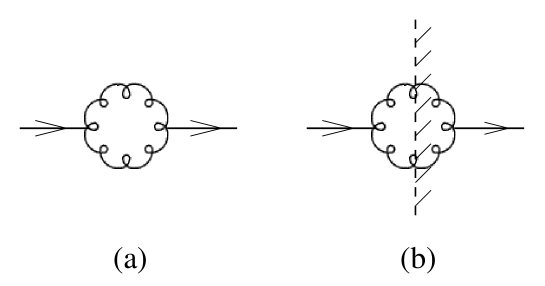
Figure 1: Feynman graphs for the retarded self-energy of $\eta^{\prime}$.

The details of their evaluation is presented in Appendix A. In the present case, it turned out that the thermal correction is negligibly small up to $T\approx 0.5\hbox{\,GeV}$. Therefore we can safely ignore it for our purposes.

Before proceeding to analyze the Boltzmann equation, we must ask if we can use the Boltzmann equation in a quark gluon plasma. In other words, can $\eta^{\prime}$ exist in a quark gluon plasma as a quasi-particle? It is possible that an excitation with the same quantum numbers as $\eta^{\prime}$ can exist in the plasma (for instance see [5]) but its width may be too broad to be a quasi particle. To be conservative, we apply the Boltzmann equation starting only from one relaxation time before the hadronization time unless the hadronization time is shorter than the relaxation time.

If the steady state is reached during the evolution, then the Boltzmann equation dictates that distribution functions become Bose-Einstein functions. In this case, the distribution of $\eta^{\prime}$ at the hadronization time will be simply the Bose-Einstein distribution with the temperature of $T_{c}\approx 0.17\hbox{\,GeV}$. This in itself is an interesting conclusion because there are surely other hadronization processes and hadronic processes that produce additional $\eta^{\prime}$. Since $\eta^{\prime}$ life time is about $1000\hbox{\,fm}$ and the mean free path in dense hadronic matter exceeds $10\hbox{\,fm}$ [5], the final $\eta^{\prime}$ multiplicity will exceed thermal model expectation.

However, local chemical equilibrium between $\eta^{\prime}$ and gluons may not be readily reached during the quark-gluon plasma evolution although quarks and gluons do reach local equilibrium very fast. Therefore, $f_{\eta^{\prime}}$ must evolve non-trivially in time even if the gluons are already locally equilibrated. To calculate such an effect, we assume that the gluon density is already thermal and rewrite the above as

$$\partial_{t}f_{\eta^{\prime}}+{\bf v}\cdot\nabla f_{\eta^{\prime}} = {1\over 4E_{P}}\int{d^{3}p\over(2\pi)^{3}2p}{d^{3}q\over(2\pi)^{3}2q}\,\left|M\right|_{gg\to\eta^{\prime}}^{2}\,(2\pi)^{4}\delta(p+q-P)$$ (13)

$${}\qquad\times f_{g}(p)\,f_{g}(q)\,\left[1-f_{\eta^{\prime}}(P)/f_{BE}(P)\right]$$

where $f_{BE}(P)=1/(e^{E_{P}/T}-1)$. Substituting the matrix element yields

$$\partial_{t}f_{\eta^{\prime}}+{\bf v}\cdot\nabla f_{\eta^{\prime}} = {\left|H_{0}\right|^{2}M^{4}_{\eta^{\prime}}\over E_{P}}\left[1-f_{\eta^{\prime}}(P)/f_{BE}(P)\right]\,\Gamma_{2}(P)$$ (14)

where the 2-body thermal phase space factor is given by

$$\Gamma_{2}(P)=\int{d^{3}p\over(2\pi)^{3}2p}{d^{3}q\over(2\pi)^{3}2q}\,(2\pi)^{4}\delta(p+q-P)f_{g}(p)\,f_{g}(q)\,$$ (15)

The evaluation of $\Gamma_{2}(P)$ can be found in Appendix B. In the Boltzmann limit,

$$\Gamma_{2}(P)={1\over 8\pi}\,e^{-E_{P}/T}$$ (16)

For simplicity, we take the Boltzmann limit from now on. As for the gluon evolution, we use hydrodynamic models with 1-D expansion to make a simple physical estimate. In terms of the space-time rapidity $\eta=(1/2)\ln((t+z)/(t-z))$, the flow velocity in the 1-D Bjorken model is given by

$$u^{\mu}=(\cosh\eta,0,0,\sinh\eta)$$ (17)

Using the ideal gas equation of motion $\epsilon=3p$ results in a simple time dependence of the temperature

$$T(\tau)=T_{0}\,\left(\tau_{0}\over\tau\right)^{1/3}$$ (18)

where $\tau=\sqrt{t^{2}-z^{2}}$ is the proper time and $T_{0}$ is the temperature at the initial (proper) time $\tau_{0}$. Further, we limit the $\eta^{\prime}$ momenta to be at the central rapidity so that $v_{z}=P_{z}/E_{P}=0$. In that case, only the time derivative term from the left hand side of the Boltzmann equation remains non-vanishing. The coordinate $z$ and the momentum $P$ merely are parameters in 1-D ordinary differential equation

$${df(t,z,P)\over dt}={\left|H_{0}\right|^{2}M^{4}_{\eta^{\prime}}\over 8\pi E_{P}}\left[e^{-E_{P}\cosh\eta/T(\tau)}-f(t,z,P)\right]$$ (19)

where we have omitted the subscript label $\eta^{\prime}$ from the distribution and $\eta$ and $T$ are functions of $t$ and $z$. This is in the form of a relaxation equation. The relaxation time is given by

$$t_{P}^{\rm rel}={8\pi E_{P}\over\left|H_{0}\right|^{2}M^{4}_{\eta^{\prime}}}=\tau_{\rm rel}\,\gamma_{P}$$ (20)

where $\tau_{\rm rel}=4.5\hbox{\,fm}$ is the relaxation time in the rest frame of the $\eta^{\prime}$ and $\gamma_{P}=E_{P}/M_{\eta^{\prime}}$ is the Lorentz $\gamma$ factor associated with the $\eta^{\prime}$ momentum. Here we used $M_{\eta^{\prime}}=0.7\hbox{\,GeV}$ in accordance with our earlier discussion. Up to the momentum of $1\,\hbox{GeV}$, the typical $\gamma$ factor does not exceed 2. Therefore the relaxation time is comparable with the typical plasma life time of $1-10\,\hbox{fm}$. The relaxation time $t_{P}^{\rm rel}$ is independent of the temperature unless $H_{0}$ and/or $M_{\eta^{\prime}}$ depends strongly on $T$.

The solution of the above equation is given by

$$f(t,z,P)=\int_{t_{\rm init}}^{t}{dt^{\prime}\over t_{P}^{\rm rel}}\,e^{-(t-t^{\prime})/t_{P}^{\rm rel}}\,f_{0}(t^{\prime},z,P)$$ (21)

with the initial condition $f(t_{\rm init},z,P)=0$ and $f_{0}(t^{\prime},z,P)=e^{-E_{P}\cosh\eta(t^{\prime},z)/T(t^{\prime},z)}$. What we are interested in is the distribution function at the hadronization time $t_{\rm had}$. In the Bjorken model, the proper time at the hadronization is given by

$$\tau_{\rm had}=\tau_{0}\,\left(T_{0}\over T_{c}\right)^{3}$$ (22)

We then take the initial proper time for the $\eta^{\prime}$ evolution to be the larger of $\tau_{0}$ and

$$\tau_{\rm init}=\tau_{\rm had}-\tau_{\rm rel}$$ (23)

The Mikowskian time and the proper time is related by

$$t=\sqrt{\tau^{2}+z^{2}}$$ (24)

Therefore, the farther away from the origin, the later the initial time is. This is due to the strong longitudinal flow and time dilation associated with it. The longitudinal flow is faster further away from the origin. It also means that at large $z$, there will be very little time between the on-set of $\eta^{\prime}$ production by fusing gluons and the hadronization time.

3 Numerical Results

To evaluate Eq. (21), we take $T_{0}=0.334\hbox{\,GeV}$ and $\tau_{0}=0.6\hbox{\,fm}$. These parameters are taken from a recent hydrodynamic study of the elliptic flow at RHIC[19]. The initial temperature corresponds to the average energy density of about $23\hbox{\,GeV}/\hbox{\,fm}^{-3}$. The hadronization proper time with these parameters is $\tau_{\rm had}=4.6\hbox{\,fm}$. Since $\tau_{\rm had}-\tau_{\rm rel}=0.1\hbox{\,fm}$ is shorter than $\tau_{0}$, we set $\tau_{\rm init}=\tau_{0}$.

Fig. 2 shows the numerical solutions with $P=0$ within the time interval $t_{\rm init}\leq t\leq t_{\rm had}$.

Figure 2: The ratio of the solution of Eq.(21) and $f_{0}=e^{-M_{0}\cosh\eta(t,z)/T(t,z)}$ at $P=0$ as a function of time. Here $M_{0}=0.958\hbox{\,GeV}$ is the vacuum $\eta^{\prime}$ mass. From the bottom, the curves correspond to the final space-time rapidities $\eta=0.0$ through $0.5$ in steps of $0.1$ at $t_{\rm had}$. Calculated with the RHIC parameters. The end points corresponds to $t_{\rm init}=\sqrt{\tau_{\rm init}^{2}+z^{2}}$ and $t_{\rm fin}=\sqrt{\tau_{\rm fin}^{2}+z^{2}}$.

In Fig. 2 we plot the ratio of our solution and what one expects from the thermal model,

$$f_{\rm vac}\equiv\exp\left(-M_{0}\cosh\eta(t,z)/T(t,z)\right)$$ (25)

where $M_{0}$ is the mass of $\eta^{\prime}$ in vacuum.

The curves in Fig. 2 starts from 0 and keeps growing. This is due to two reasons. One, the solution itself overshoots the equilibrium distribution $f_{0}$ (which has the same in-medium $M_{\eta^{\prime}}=0.7\hbox{\,GeV}$) because the temperature is a decreasing function of time. Initially the slope $df/dt$ is too steep for the eventual temperature of $T_{c}=0.17\hbox{\,GeV}$. Two, since the in-medium mass is 30 % smaller than the vacuum mass, $f_{\rm vac}$ in Eq. (25) decreases much faster than either $f$ or $f_{0}$ as $t$ increases.

It is also apparent that for larger $\eta$ or equivalently larger $z$, there is not enough time between $t_{\rm init}=\sqrt{\tau_{\rm init}^{2}+z^{2}}$ and $t_{\rm fin}=\sqrt{\tau_{\rm fin}^{2}+z^{2}}$ for the solution to grow over $f_{\rm vac}$. Consequently, the enhancement of $dN_{\eta^{\prime}}/dy$ at the mid-rapidity ($y=0$)

$${\left(dN_{\eta^{\prime}}/dy\right)_{f}\over\left(dN_{\eta^{\prime}}/dy\right)_{f_{\rm vac}}}\approx 2.5\ \ \ \ \hbox{(RHIC)}$$ (26)

is not as large as the enhancement of $f$ at $\eta=0$. Here we used

$$\left.{dN_{\eta^{\prime}}\over dy}\right|_{y=0}=\int{d^{2}P_{T}\over(2\pi)^{3}}\,E_{P}\int d^{3}x\,f(t_{\rm had},z,P_{T})$$ (27)

This enhancement factor is not particularly sensitive to the initial temperature. Keeping $\tau_{0}$ fixed, the ratio is 1.8 at $T_{0}=0.3\hbox{\,GeV}$, increases up to 2.6 at $T_{0}=0.35\hbox{\,GeV}$ and then decreases to 2.2 at $T_{0}=0.4\hbox{\,GeV}$.

One should note that this is on top of other processes that produce $\eta^{\prime}$ at the hadronization and in later times. Therefore, this result definitely indicates a large enhancement in the $\eta^{\prime}$ yield due to the thermal gluon fusion process at RHIC.

At LHC, the initial temperature can reach $T_{0}=1\hbox{\,GeV}$. Accordingly, the hadronization takes place much later, $\tau_{\rm had}=10-20\hbox{\,fm}$ even though the equilibration time is shorter, $\tau_{0}\approx 0.1\hbox{\,fm}$ [22]. Therefore the rate of the change in the temperature is slower than the rate at RHIC (recall $T=T_{0}(\tau_{0}/\tau)^{1/3}$). This implies that even though the initial temperature is much higher than the temperature at RHIC, the enhancement factor may not be much different. With $\tau_{0}$ fixed at $0.1\hbox{\,fm}$, we get

$${\left(dN_{\eta^{\prime}}/dy\right)_{f}\over\left(dN_{\eta^{\prime}}/dy\right)_{f_{\rm vac}}}\approx 2-3\ \ \ \ \hbox{(LHC)}$$ (28)

between $T_{0}=0.5\hbox{\,GeV}$ and $T_{0}=1.0\hbox{\,GeV}$. The maximum enhancement factor 3 is reached at $T_{0}=0.6\hbox{\,GeV}$.

At SPS, the enhancement factor is more sensitive to the initial temperature. Keeping $\tau_{0}=0.8\hbox{\,fm}$ [19], the ratio increases as the temperature increases within $0.2\hbox{\,GeV}\leq T_{0}\leq 0.25\hbox{\,GeV}$

$$0.3\,\,\vbox{\hbox{$\buildrel\displaystyle<\over{\sim}$}}\,\,{\left(dN_{\eta^{\prime}}/dy\right)_{f}\over\left(dN_{\eta^{\prime}}/dy\right)_{f_{\rm vac}}}\,\,\vbox{\hbox{$\buildrel\displaystyle<\over{\sim}$}}\,\,1.1\ \ \ \ \hbox{(SPS)}$$ (29)

Since $\eta^{\prime}$ decays to $\eta\pi\pi$ in 65 % of the times, one may ask if this SPS result is compatible with the $\eta$ multiplicity measurement by WA80 and the low mass dilepton spectrum measured by CERES. Thermal ratio of $\eta^{\prime}$ and $\eta$ within the Bjorken scenario is 17 %. Therefore one would expect that about 11 % of $\eta$ comes from $\eta^{\prime}$ decay. Doubling that would indicate about 10 % increase in the $\eta$ multiplicity. However, at present the experimental uncertainty is bigger than than 10 % [20, 21].

More detailed information than the yield can be obtained in the transverse momentum distribution shown in Fig. 3. There is a clear difference between our calculation and the thermal distribution. As one can see, the dependence of the solution Eq. (21) on $T_{0}$ and $\tau_{0}$ is non-trivial. Since the simple 1-D model we employ does not take into account the transverse flow, the slope parameter of the $p_{T}$ spectra in Fig. 3 should be taken as qualitative estimates rather than quantitative predictions.

Figure 3: The transverse momentum spectrum of $\eta^{\prime}$ calculated with the solution Eq. (21) (solid line) and the thermal $e^{-E^{0}_{P}\cosh\eta/T_{c}}$ (broken line) where $E^{0}_{P}$ is calculate with the vacuum $\eta^{\prime}$ mass. For the top two lines, we used $T_{0}=1\hbox{\,GeV}$ and $\tau_{0}=0.1\hbox{\,fm}$ estimated for LHC in Ref.[22]. SPS and RHIC parameters are $T_{0}=0.257\hbox{\,GeV},T_{0}=0.334\hbox{\,GeV}$ and $\tau_{0}=0.8\hbox{\,fm},\tau_{0}=0.6\hbox{\,fm}$ respectively [19]. Transverse expansion is not taken into account.

4 Discussion and Conclusion

In this paper, we calculated the yield and the momentum spectrum of the flavor singlet $\eta^{\prime}$ mesons produced by the fusion of thermal gluons. It is shown above that at RHIC and LHC, there is a significant enhancement in $\eta^{\prime}$ yield. Furthermore, the $p_{T}$ spectrum of $\eta^{\prime}$ shows an interesting deviation from the $M_{T}$ scaling. The on-set of the deviation from the naive $M_{T}$ scaling contains information on the initial conditions such as the initial temperature and the thermalization time. This may be feasible since $\eta^{\prime}$ has a long life-time and a long mean free path.

Further implication of our result includes the low mass dilepton enhancement. The branching ratio of $\eta^{\prime}\to\eta\pi\pi$ is 65 %. A large number of $\eta^{\prime}$ results in a sizable increase in $\eta$ multiplicity which in turn gives rise to the $\eta$ Dalitz peak in the dilepton invariant mass spectrum. At SPS, the enhancement is not significant enough to be noticed. But at RHIC and LHC, there can be a substantial increase of the peak. Another observable where $\eta^{\prime}$ enhancement plays a role is the HBT correlation. As shown in Ref. [23], enhanced $\eta^{\prime}$ production reduces the strength of the HBT correlation at small $p_{T}$.

The above conclusions are based on the effective $gg\eta^{\prime}$ vertex deduced by Atwood and Soni, the Kinetic (Boltzmann) equation and also the following assumptions:

• The gluons are locally thermalized and follow the hydrodynamic evolution.

• The strength of $gg\eta^{\prime}$ vertex is independent of the temperature.

• The mass of $\eta^{\prime}$ involved in this process is lower than the vacuum value since only the $s$ quark loop is involved in the anomalous coupling.

• Kinetic equation is valid in this regime.

As to the validity of the hydrodynamics, the measurements of the elliptic flow indicate the existence of collective motion. Whether this implies thermal and chemical equilibrium is not entirely certain. Since our result indicates that the $\eta^{\prime}$ density is proportional to the square of the gluon density, the measured $\eta^{\prime}$ $dN/dy$ must reflect the underlying gluon distribution be it thermal or the gluon $x$ distribution function. For instance, if the plasma is gluon dominated right up to the hadronization, then one should see even more $\eta^{\prime}$ than what we have estimated.

One may also question the validity of the 1-D expansion model we employed. The full 3-D calculation with a realistic equation of state is clearly out of the scope of this paper. However, our main results should be robust since faster falling temperature makes the $\eta^{\prime}$ distribution overshoot even more.

The temperature dependence of the $gg\eta^{\prime}$ vertex and properties of $\eta^{\prime}$ itself are at present not fully understood. In this study, we made simple assumptions to make a progress. As we argued in Introduction, the strength of $gg\eta^{\prime}$ vertex will not vanish as the strength of $\pi^{0}\gamma\gamma$ vertex does at $T_{c}$. If one accepts the rough estimate Eq. (5) at the face value, then the strength of the $gg\eta^{\prime}$ coupling could even be larger than $H_{0}$. The exact temperature dependence of the vertex, however, has yet to be worked out. The crucial question is then: What exactly is the relation between $H_{0}$ and $M_{\eta^{\prime}}$ as a function of temperature? High statistics measurement of $\eta^{\prime}$ spectrum can potentially answer this question by employing the ideas developed in this paper.

The kinetic equation description is valid when the mean free path is much larger than any other length scale. This is certainly the case. The mean free time of the $\eta^{\prime}$ is longer than $4\hbox{\,fm}$. The dense medium at $T=300\hbox{\,MeV}$ has much smaller inter-particle distance. The effect of inclusion of other processes such as $q\bar{q}\to\eta^{\prime}$ can be roughly estimated by raising the value of $H_{0}$. In our calculation, this leads to more $\eta^{\prime}$ production by shortening $t_{\rm rel}$.

In summary, we have shown that $\eta^{\prime}$ is a good probe of the gluons density using the recently proposed $gg\eta^{\prime}$ effective vertex. Other application along the same idea includes the investigation of the in-medium properties of $\eta^{\prime}$ and its possible link to the fate of the axial anomaly in a quark-gluon plasma. It will be also interesting to study formation of $\eta^{\prime}$ within gluon jets. These and other aspects are currently under investigation.

Appendix A Real Part of the $\eta^{\prime}$ Self-Energy in Thermal Gluons

The Feynman diagrams for the one-loop retarded self-energy of the $\eta^{\prime}$ in equilibrium is given in Fig. 1. These can be calculated in many ways. In this paper, we adopt the set of Feynman rules derived in Ref. [24]. The diagrams then corresponds to the expressions

$$\Sigma_{a}(P)={-i\over 2}\int{d^{4}p\over(2\pi)^{4}}\,{d^{4}q\over(2\pi)^{4}}\,(2\pi)^{4}\delta(p+q-P)\,(\hbox{Tr\,}\,M(p,q)^{2})\,G(p)\,G(q)$$ (30)

and

$$\Sigma_{b}(P)={-i\over 2}\int{d^{4}p\over(2\pi)^{4}}\,{d^{4}q\over(2\pi)^{4}}\,(2\pi)^{4}\delta(p+q-P)\,(\hbox{Tr\,}\,M(p,q)^{2})\,\Delta_{+}(p)\,\Delta_{+}(q)$$ (31)

where

$$G(p)={i\over p^{2}+i\epsilon}+n_{BE}(p)2\pi\delta(p^{2})$$ (32)

and

$$\Delta_{+}(p)=\theta(p^{0})2\pi\delta(p^{2})+n_{BE}(p^{0})2\pi\delta(p^{2})$$ (33)

The prefactor $1/2$ comes from the fact that the two intermediate gluons are identical. Using these propagators, it is clear that the real part of the self-energy comes only from the diagram (a). Hence we concentrate on evaluation of (a) from now on.

First, we evaluate the vertex trace

$$(\hbox{Tr\,}\,M(p,q)^{2})\, = \sum_{ab}\delta^{ab}\sum_{\lambda,\gamma}M^{*}_{\lambda\gamma}M^{\vphantom{*}}_{\lambda\gamma}$$ (34)

$$= 8H_{0}^{2}\,\epsilon_{\alpha\beta\mu\nu}\,\epsilon^{\alpha\beta\rho\sigma}\,p^{\mu}q^{\nu}p_{\rho}q_{\sigma}$$

$$= 16H_{0}^{2}\,\left((p\cdot q)^{2}-p^{2}q^{2}\right)$$

using the identities

$$\sum_{\lambda}(\epsilon_{p}^{\alpha})_{\lambda}^{*}(\epsilon_{p}^{\zeta})_{\lambda}=-g^{\alpha\zeta}+ap^{\alpha}p^{\zeta}$$ (35)

and (36)

$$\epsilon_{\alpha\beta\mu\nu}\,\epsilon^{\alpha\beta\rho\sigma}=2\left(g^{\mu}_{\sigma}\,g^{\nu}_{\rho}-g^{\mu}_{\rho}\,g^{\nu}_{\sigma}\right)$$

The $ap^{\alpha}p^{\zeta}$ term does not contribute due to the anit-symmetric property of $\epsilon_{\alpha\beta\mu\nu}$. Then

$$\Sigma_{a}(P) = {-8iH_{0}^{2}}\int{d^{4}p\over(2\pi)^{4}}\,{d^{4}q\over(2\pi)^{4}}\,(2\pi)^{4}\delta(p+q-P)\,\left((p\cdot q)^{2}-p^{2}q^{2}\right)\,G(p)\,G(q)$$ (37)

$$= {-8iH_{0}^{2}}\int{d^{4}p\over(2\pi)^{4}}\,\left((p\cdot(P-p))^{2}-p^{2}(P-p)^{2}\right)\,G(p)\,G(P-p)$$

The zero-temperature part of this diagram is badly divergent. In view of the effective theory nature of this vertex, we will simply drop the zero-temperature part in this calculation. The thermal part can be separated into two parts,

$$\Sigma_{a}(P)=\Sigma_{a,1}(P)+\Sigma_{a,2}(P)$$ (38)

where

$$\Sigma_{a,1}(P) = {-16iH_{0}^{2}}\int{d^{4}p\over(2\pi)^{4}}\,(p\cdot P)^{2}\,{i\over M^{2}-2P\cdot p+i\epsilon}\,n(p)2\pi\delta(p^{2})$$ (39)

and

$$\Sigma_{a,2}(P) = {-8iH_{0}^{2}}\int{d^{4}p\over(2\pi)^{4}}\,(p\cdot P)^{2}\,n(E_{P-p})2\pi\delta(M^{2}-2P{\cdot}p)\,n(p)2\pi\delta(p^{2})$$ (40)

and we used the on-shell conditions $p^{2}=0$ and $P^{2}=M^{2}$.

The real part of the self-energy comes only from $\Sigma_{a,1}(P)$.

$${\rm Re}\,\Sigma_{\rm ret}(P) = {\rm Re}\,\Sigma_{a,1}(P)$$

$$= {16H_{0}^{2}}\int{d^{4}p\over(2\pi)^{4}}\,(p\cdot P)^{2}\,{\rm PP}\,{1\over M^{2}-2P\cdot p}\,n(p)2\pi\delta(p^{2})$$

$$= -{4H_{0}^{2}M^{2}}\int{d^{4}p\over(2\pi)^{4}}\,n(p)2\pi\delta(p^{2})$$

$${}+{4H_{0}^{2}M^{4}}\int{d^{4}p\over(2\pi)^{4}}\,{\rm PP}\,{1\over M^{2}-2P\cdot p}\,n(p)2\pi\delta(p^{2})$$

where ${\rm PP}$ signifies the principal part.

For simplicity, we orient $P^{\mu}=(E_{P},0,0,P)$ and approximate the Bose-Einstein factor by a Boltzmann factor

$$n(p)\approx e^{-p/T}$$ (42)

Then

$${\rm Re}\,\Sigma(P) \approx -{4H_{0}^{2}M^{2}}{1\over(2\pi)^{2}}\int dp\,p\,e^{-\left|p\right|/T}$$

$${}+{4H_{0}^{2}M^{4}}\int{d^{4}p\over(2\pi)^{4}}\,{\rm PP}\,{1\over M^{2}-2P\cdot p}\,e^{-\left|p\right|/T}\,2\pi\delta(p^{2})$$

$$= -{4H_{0}^{2}M^{2}}{T^{2}\over(2\pi)^{2}}\Bigg{[}1-$$

$${}+{M^{2}\over 4PT^{2}}\int dp\,e^{-p/T}\left\{\ln\left|M^{2}-2Ep+2Pp\over M^{2}-2Ep-2Pp\right|+\ln\left|M^{2}+2Ep+2Pp\over M^{2}+2Ep-2Pp\right|\right\}\Bigg{]}$$

The result can be expressed in terms of the exponential integral functions

$${\rm Re}\,\Sigma_{\rm ret}(P) = -M^{2}{4H_{0}^{2}T^{2}\over(2\pi)^{2}}\left(1-{M^{2}\over 4PT}A(P)\right)$$ (44)

where

$$A(P) = {M^{2}}\,e^{-(P+E_{P})/2T}\,\Bigg{[}-e^{E_{P}/T}\,\hbox{Ei}\left({\frac{P-E_{P}}{2\,T}}\right)+e^{P/T}\,\hbox{Ei}\left({\frac{-P+E_{P}}{2\,T}}\right)$$ (45)

$$\quad\qquad{}+e^{(P+E_{P})/T}\,\hbox{Ei}\left({\frac{-\left(P+E_{P}\right)}{2\,T}}\right)-\hbox{Ei}\left({\frac{P+E_{P}}{2\,T}}\right)\Bigg{]}$$

Numerically, between $T=0.17\hbox{\,GeV}$ and $T=1.0\hbox{\,GeV}$, the second term is important only near $P=0$. Therefore we approximate the above with

$${\rm Re}\,\Sigma_{\rm ret}(P) \approx \Sigma_{\rm ret}(P=0)$$

$$= -M^{2}{4H_{0}^{2}T^{2}\over(2\pi)^{2}}\left(1-{M^{2}\over 4T}\left(e^{M/2T}\hbox{Ei}(-M/2T)+e^{-M/2T}\hbox{Ei}(M/2T)\right)\right)$$

We can self-consistently determine $M$ by solving the following equation for $M$ with $M_{0}=0.7\hbox{\,GeV}$:

$$M^{2}=M_{0}^{2}+{\rm Re}\,\Sigma_{\rm ret}(0)$$ (47)

Numerically solution of this equation indicates that $M(T)$ is a slow varying function of $T$. At $T=0.17\hbox{\,GeV}$, $M(T)=0.7\hbox{\,GeV}$ is indistinguishable from $M_{0}$. Even at $T=0.5\hbox{\,GeV}$, $M(T)=0.68\hbox{\,GeV}$. Only around $T=1\hbox{\,GeV}$, $M(T)=0.64\hbox{\,GeV}$ is appreciably different from $M_{0}$. However, at this temperature, our Boltzmann approximation is no longer appropriate. We can ignore the temperature dependence of the $\eta^{\prime}$ mass for our estimates.

Appendix B 2 Body Thermal Phase Space

We start from the expression

$$\Gamma_{2}(P)=\int{d^{3}p\over(2\pi)^{3}2p}{d^{3}q\over(2\pi)^{3}2q}\,(2\pi)^{4}\delta(p+q-P)f_{g}(p)\,f_{g}(q)\,$$ (48)

Carrying out the $d^{3}p$ integral and the $q$ angle integral yields

$$\Gamma_{2}(P) = {1\over 4}\int{d^{3}q\over(2\pi)^{3}q\left|{\bf P}-{\bf q}\right|}\,(2\pi)\delta(\left|{\bf P}-{\bf q}\right|+q-E_{P})f_{g}(\left|{\bf P}-{\bf q}\right|)\,f_{g}(q)$$ (49)

$$= {1\over 4}{1\over 2\pi}{1\over\left|{\bf P}\right|}\,\int_{q_{\rm min}}^{q_{\rm max}}dq\,f_{g}(E_{P}-q)\,f_{g}(q)$$

where

$$\displaystyle q_{\rm min}={M^{2}\over 2(E_{P}+P)}$$ (50)

and (51)

$$\displaystyle q_{\rm max}={M^{2}\over 2(E_{P}-P)}$$

Using the Bose-Einstein functions for $f$, we get

$$\Gamma_{2}(P) = f_{BE}(E_{P})\,{T\over 8\pi\left|\bf P\right|}\bigg{[}\ln\left(e^{q_{\rm max}/T}-1\right)-\ln\left(e^{q_{\rm min}/T}-1\right)$$ (52)

$$\qquad{}+\ln\left(e^{E_{P}/T}-e^{q_{\rm min}/T}\right)-\ln\left(e^{E_{P}/T}-e^{q_{\rm max}/T}\right)\bigg{]}$$

In $T\to 0$ limit, we recover the Boltzmann result

$$\Gamma_{2}(P)={1\over 8\pi}e^{-E_{P}/T}$$ (53)

References

• [1] A.Β A.Β Belavin, A.Β M.Β Polyakov, A.Β S.Β Shvarts and Y.Β S.Β Tyupkin, Phys.Β Lett.Β B 59, 85 (1975).
• [2] E.Β Witten, Nucl.Β Phys.Β B 156, 269 (1979).
• [3] G.Β Veneziano, Nucl.Β Phys.Β B 159, 213 (1979).
• [4] G. ’t Hooft, Phys.Β Rev.Β Lett.Β  37, 8 (1976).
• [5] J.Β Kapusta, D.Β Kharzeev and L.Β McLerran, Phys.Β Rev.Β D 53, 5028 (1996)
• [6] A.Β L.Β Kagan and A.Β A.Β Petrov, β€œΞ·β€²superscriptπœ‚β€²\eta^{\prime} production in B decays: Standard model vs. new physics,” hep-ph/9707354.
• [7] D.Β Atwood and A.Β Soni, Phys.Β Lett.Β B 405, 150 (1997)
• [8] T.Β Muta and M.Β Yang, Phys.Β Rev.Β D 61, 054007 (2000)
• [9] A.Β Ali, J.Β Chay, C.Β Greub and P.Β Ko, Phys.Β Lett.Β B 424, 161 (1998)
• [10] W.Β Hou and B.Β Tseng, Phys.Β Rev.Β Lett.Β  80, 434 (1998)
• [11] P.Β H.Β Damgaard, H.Β B.Β Nielsen and R.Β Sollacher, Nucl.Β Phys.Β B 414, 541 (1994)
• [12] R.Β D.Β Pisarski, T.Β L.Β Trueman and M.Β H.Β Tytgat, Phys.Β Rev.Β D 56, 7077 (1997)
• [13] S.Β P.Β Kumar, D.Β Boyanovsky, H.Β J.Β de Vega and R.Β Holman, Phys.Β Rev.Β D 61, 065002 (2000)
• [14] H.Β Itoyama and A.Β H.Β Mueller, Nucl.Β Phys.Β B 218, 349 (1983).
• [15] T.Β Schafer, Phys.Β Lett.Β B 389, 445 (1996)
• [16] P.Β Elmfors, Nucl.Β Phys.Β B 487, 207 (1997)
• [17] S.Β Jeon, Phys.Β Rev.Β D 52, 3591 (1995)
• [18] S.Β Jeon and L.Β G.Β Yaffe, Phys.Β Rev.Β D 53, 5799 (1996)
• [19] P.Β F.Β Kolb, P.Β Huovinen, U.Β Heinz and H.Β Heiselberg, Phys.Β Lett.Β B 500, 232 (2001)
• [20] A.Β Lebedev et al. [WA80 Collaboration.], Nucl.Β Phys.Β A 566, 355C (1994).
• [21] R.Β Albrecht et al. [WA80 Collaboration.], Phys.Β Lett.Β B 361, 14 (1995)
• [22] K.Β J.Β Eskola, K.Β Kajantie, P.Β V.Β Ruuskanen and K.Β Tuominen, Nucl.Β Phys.Β B 570, 379 (2000)
• [23] S.Β E.Β Vance, T.Β Csorgo and D.Β Kharzeev, Phys.Β Rev.Β Lett.Β  81, 2205 (1998)
• [24] S.Β Jeon and P.Β J.Β Ellis, Phys.Β Rev.Β D 58, 045013 (1998)