Solitons in nonlocal chiral quark models

Properties of hedgehog solitons in a chiral quark model with nonlocal regulators are described. We discuss the formation of the hedgehog soliton, the quantization of the baryon number, the energetic stability, the gauging and construction of Noether currents with help of path-ordered $P$-exponents, and the evaluation of observables. The issue of nonlocality is thoroughly discussed, with a focus on contributions to observables related to the Noether currents. It is shown that with typical model parameters the solitons are not far from the weak nonlocality limit. The methods developed are applicable to solitons in models with separable nonlocal four-fermion interactions.

, , and

^a The H. Niewodniczański Institute of Nuclear Physics, ul. Radzikowskiego 152, PL-31342 Kraków, Poland 

^b Faculty of Education, University of Ljubljana and J. Stefan Institute, Jamova 39, P.O. Box 3000, 1001 Ljubljana, Slovenia 

^c Service de Physique Théorique, Centre d’Etudes de Saclay, F-91191 Gif-sur-Yvette Cedex, France 

^d ECT^∗, Villa Tombosi, I-38050 Villazano (Trento), Italy 

PACS: 12.39.-x, 12.39.Fe, 12.40.Yx

1 Introduction

Effective chiral quark models have been used extensively to describe the low-energy phenomena associated with the dynamical breaking of the chiral symmetry. Of particular interest are models which include the Dirac sea of quarks, since they allow for a common description of mesons and baryons. The models share the feature of having an attractive four-quark interaction which is either:

• postulated [1];

• derived from a model of the underlying QCD structure of the vacuum [2, 3, 4, 5];

• obtained by modeling the effective gluon propagator and using Schwinger-Dyson techniques [6, 7];

• derived from QCD inspired models [8, 9, 10, 11].

For extensive reviews with a focus on solitons, and numerous additional references, see [4, 12, 13]. The four-quark interaction leads to the chiral symmetry breaking, which is, in the framework of these models, the key dynamical ingredient.

The various models fall into two categories: local models, where the four-quark interaction is point-like and where ultra-violet divergences are removed by introducing cut-offs in the quark loop, and nonlocal models, where the four-quark interaction is smeared, such that all Feynman diagrams in the theory are finite. Nonlocal models arise naturally in several approaches to low-energy quark dynamics, such as the instanton-liquid model [14] or Schwinger-Dyson resummations [6]. For the derivations and farther applications of nonlocal quark models see, e.g.,[11, 15, 16, 17, 18, 19, 20, 21, 22, 23, 24, 25, 26, 27, 28, 29].

Considerable effort has been exerted to describe baryons as solitons of effective chiral quark models [12, 30, 31, 32, 33, 34, 35, 36]. The solitons appear as bound states of quarks. Except for our earlier-reported work [37, 38], solitons have so far only been obtained from local models, which typically use the Schwinger proper-time or the Pauli-Villars regularization of the Dirac sea [12, 39]. One problem encountered with the proper-time regularization, by far the most commonly used, is that the solitons turn out to be unstable unless the auxiliary sigma and pion fields, introduced in the process of semi-bosonization, are constrained to lie on the chiral circle [40, 41]. Such a constraint is external to the model itself. Nonlocal models do not suffer from this instability: we have shown [37, 38] that stable solitons exist in a chiral quark model with nonlocal interactions without the extra chiral-circle constraint. In fact, we find appreciable deviations from the chiral circle. Furthermore, in local models, the regularization is applied only to the real (non-anomalous) part of the Euclidean quark-loop term. The finite imaginary (anomalous) part is left unregularized in order to properly describe anomalous processes [42]. One may view such a division as rather artificial, and we find it quite appealing that, with nonlocal regulators, both the real and imaginary parts of the action are treated on equal footing. Moreover, the anomalies are preserved [16, 17, 19, 24, 25] and the charges are properly quantized [37]. Finally, the momentum-dependent regulator makes the theory finite to all orders in the $1/N_{c}$ expansion. This is in contrast to local models, where inclusion of higher-order-loop effects requires extra regulators [43, 44, 45, 46, 47] and the predictive power is diminished.

The above-mentioned virtues of nonlocal models do not come for free. Two complications arise. First, soliton calculations require an extra integration over an energy variable, which has to be performed numerically. Second, the Noether currents in nonlocal models acquire extra contributions, which are, however, needed to conserve the Noether currents and anomalies. Nevertheless, an ambiguity remains: the transverse parts of currents are not fixed by current conservation and their choice is effectively part of the model building. This problem has been known for a long time in nuclear physics, where the transverse part of the meson-exchange currents is ambiguous [20, 21]. It is not possible to get rid of this ambiguity in gauging nonlocal models. An ideal solution would be to first gauge the underlying theory (e.g. the instanton model of the QCD vacuum), and then to derive an effective gauged quark model. This has not been attempted so far, so that in effective nonlocal quark models we need to deal with transverse currents which are not uniquely defined. Fixing these currents is a part of the model building.

In this paper we demonstrate the existence of solitons and we give the description of formal and technical aspects of constructing solitons in nonlocal chiral quark models. We do not aim for an accurate phenomenology of the nucleon and the $\mathchar 1\relax$ resonance. It is known from the experience gained in local models that, in addition to the mean-field approximation applied in our work, many other effects can and should be included: the projection of the center-of-mass motion and angular-momentum, [48, 49, 50, 51, 52], the rotational $1/N_{c}$ corrections [53, 54], inclusion of other degrees of freedom such as vector mesons [34, 55] or color-dielectric fields [56]. These may considerably alter and improve the results. We stress that the methods which we describe in this paper are applicable to all models with separable nonlocal four-fermion interactions provided that it is possible to perform an analytic continuation in the four-momentum close to zero, as explained in Sect. 2.4.

The existence of stable solitons in nonlocal models has been briefly reported in Refs. [37, 38]. In the present work we describe in greater detail how the soliton is constructed and how the valence orbit is defined (Sect. 2.4). The determination of the model parameters is described in Sect. 3. The physical properties of the soliton and its energetic stability are analyzed in Sect. 4. An important and novel feature of this paper concerns the gauging of the nonlocal model and the construction of Noether currents. In Sect. 5, we apply the technique of path-ordered $P$-exponents and we obtain general expressions for currents in the soliton background. Interesting results follow: the properties of the soliton, which are related to currents at zero momenta (charges, $g_{A}$, and in general $n$-point Green functions with vanishing momenta on external legs) do not depend on the choice of the path in the $P$-exponent, and are thus universal. On the other hand, observables which probe the soliton at non-zero momenta (form-factors, magnetic moments) do depend on the gauging prescription. However, in the cases we have explored, the contributions of the nonlocal parts of currents are small, in particular for sufficiently large solitons. In Sect. 6 we apply two prescriptions to compute observables: straight-line paths in the $P$-exponents and the weak-nonlocality limit, where the energy scale of the regulator is assumed to be parametrically much larger than the other scales in the problem.

The many-body techniques applied in our work are inherited from the experience acquired with local models. In particular, the nucleon is derived from the hedgehog soliton by cranking. We calculate the electric isoscalar radius, the isovector magnetic moment an the isovector magnetic radius. These quantities do not depend dynamically on cranking [57]. They are much simpler to evaluate numerically, involving single spectral sums, than the moment of inertia, isovector electric radius, or the isoscalar magnetic properties, which involve double spectral sums.

Appendix A contains a detailed account of the gauging method. Appendix B describes the construction of general Noether currents. Explicit forms for the straight-line $P$-exponents are given in App. C and the forms obtained from the weak-nonlocality limit are given in App. D. Expressions needed for the evaluation of observables are displayed in App. E.

2 The model

This section describes the model used to calculate the solitons. We derive the basic formulas, such as the Euler-Lagrange equations, and the expressions for the baryon number and energy. We discuss the construction of the valence orbit, which is non-trivial in nonlocal models [37].

2.1 The action

The model is defined by the Euclidean action

$$I=\intop d_{4}x\;\left[\bar{q}\left(-i\partial_{\mu}\gamma_{\mu}+m\right)q-\frac{G^{2}}{2}\left(\bar{\psi}\mathchar 0\relax_{a}\psi\right)^{2}\right]\;,$$ (1)

where $q\left(x\right)$ is the quark field, $m$ the current quark mass, $\gamma_{\mu}=\gamma^{\mu}=\left(i\beta,\vec{\gamma}\right)$ are the antihermitian (Euclidean) Dirac matrices, and $\mathchar 0\relax_{0}=1$, $\mathchar 0\relax_{a}=i\gamma_{5}\tau_{a}$ define the coupling in the scalar and pseudoscalar $q\bar{q}$ channels. We work with $N_{f}=2$ flavors. The coupling constant $G$ has the dimension of inverse energy. The delocalized quark field, $\psi\left(x\right)$, is related to the quark field $q\left(x\right)$ by a regulator $r$, which is diagonal in the momentum space:

$$\psi\left(x\right)=\left\langle x|\psi\right\rangle=\left\langle x\left|r\right|q\right\rangle=\frac{1}{\mathchar 10\relax}\sum_{k}r_{k}e^{ik\cdot x}q_{k}\;,$$ (2)

where $\mathchar 10\relax=\intop d_{4}x$ is the Euclidean space-time volume.

Our calculations use either a Gaussian (as first considered in Refs. [20, 21]) or a monopole [58] form for the regulator:

$$r_{k}=e^{-\frac{k^{2}}{2\mathchar 3\relax^{2}}}\;\;\;\left({\rm Gaussian}\right),\;\;\;\;\;r_{k}=\frac{1}{1+\frac{k^{2}}{2\mathchar 3\relax^{2}}}\;\;\;\left({\rm monopole}\right)\;.$$ (3)

The action (1) is easily cast into the form

$$I = \frac{1}{\mathchar 10\relax}\sum_{k}\bar{q}_{k}\left(k_{\mu}\gamma_{\mu}+m\right)q_{k}$$ (4)

$$-\frac{G^{2}}{2\mathchar 10\relax^{3}}\sum_{k_{1}k_{2}k_{3}k_{4}}\delta_{k_{1}+k_{3},k_{2}+k_{4}}\;r_{k_{1}}r_{k_{2}}r_{k_{3}}r_{k_{4}}\;\left(\bar{q}_{k_{1}}\mathchar 0\relax_{a}q_{k_{2}}\right)\left(\bar{q}_{k_{3}}\mathchar 0\relax_{a}q_{k_{4}}\right)\,.$$

The regulators appearing in the four-quark interaction have a separable form in momentum space. The separability of the quark interaction is also present in the instanton-liquid model [4, 5].

Soliton calculations are more easily performed by using the equivalent bosonized form of the action (1):

$$I\left(S,P\right)=-{\rm Tr}\ln\left(-i\partial_{\mu}\gamma_{\mu}+m+r\,\mathchar 8\relax\,r\right)+\frac{1}{2G^{2}}\intop d_{4}x\left(S^{2}+P_{a}^{2}\right),$$ (5)

where

$$\mathchar 8\relax\left(x\right)=S\left(x\right)+i\gamma_{5}P_{a}\left(x\right)\tau_{a}$$ (6)

is the local chiral field which is the dynamical variable of the system. The trace in Eq. (5) is over color, flavor, Dirac indices, and space-time. The chiral fields represent the following expectation values of bilinear forms of the quark fields:

$$S\left(x\right) = -G^{2}\langle\bar{\psi}\left(x\right)\psi\left(x\right)\rangle=-G^{2}\left\langle\bar{q}\left|r\right|x\right\rangle\left\langle x\left|r\right|q\right\rangle,\;\;$$

$$P_{a}\left(x\right) = -G^{2}\langle\bar{\psi}\left(x\right)i\gamma_{5}\tau_{a}\psi\left(x\right)\rangle=-G^{2}\left\langle\bar{q}\left|r\right|x\right\rangle i\gamma_{5}\tau_{a}\left\langle x\left|r\right|q\right\rangle.$$ (7)

Since stationary solitons involve time-independent $S$ and $P$ fields, it is more useful to express the action in terms of the Dirac Hamiltonian

$$h=\frac{\vec{\alpha}\cdot\vec{\nabla}}{i}+\beta m+\beta r\,\mathchar 8\relax\,r,$$ (8)

bearing in mind, however, that the regulator makes the Dirac Hamiltonian dependent (although diagonal) on the energy variable. The action (5) becomes

$$I=-{\rm Tr}\ln\left(\partial_{\tau}+h\right)+\frac{1}{2G^{2}}\intop d_{4}x\left(S^{2}+P_{a}^{2}\right),$$ (9)

where $\tau$ is the Euclidean time variable.

2.2 The hedgehog soliton

Our use of the model action (9) is the same as in other hedgehog soliton calculations: we treat the $S$ and $P$ fields classically, thus keeping the leading-order contribution in the number of colors, $N_{c}$. Interestingly, in nonlocal models the next-to-leading-order corrections are found to be surprisingly small in the vacuum sector [26, 59, 60, 61, 62, 63].

We seek a stationary point of the action, or, more precisely, a minimum of the energy for time-independent chiral fields with a hedgehog shape

$$S\left(\vec{x}\right)=S\left(|\vec{x}|\right),\quad P_{a}\left(\vec{x}\right)=\widehat{x}_{a}P\left(|\vec{x}|\right),$$ (10)

where $\widehat{x}_{a}=x_{a}/|\vec{x}|$. Asymptotically, far from the soliton, the fields recover their vacuum values $S\left(x\right)=M$ and $P_{a}\left(x\right)=0$. We shall refer to the vacuum value $M$ of the scalar field as the constituent quark mass (see the discussion of what we mean by the quark mass in Sect. 3.1). The soliton represents a bound state of $N_{c}=3$ quarks occupying a valence orbit with the grand spin and parity $G^{P}=0^{+}$, where the grand spin $\vec{G}=\vec{J}+\vec{I}$ is the sum of the total angular momentum and isospin [30, 32], together with a Dirac sea which is polarized by the hedgehog field.

2.3 The energy-dependent quark orbits

The regulator acts as a differential operator, $r\equiv r\left(-\partial_{\tau}^{2}-\vec{\nabla}^{2}\right)$. It introduces a nonlocal interaction between the quarks and the chiral fields. For time-independent chiral fields $\mathchar 8\relax$, defined in Eq. (6), the Dirac operator is diagonal in the energy representation,

$$\left(\partial_{\tau}+h\right)\left|\omega\right\rangle=\left(i\omega+h(\omega^{2})\right)\left|\omega\right\rangle,$$ (11)

where $h\left(\omega^{2}\right)$ is the energy-dependent Dirac Hamiltonian:

$$h(\omega^{2})=\frac{\vec{\alpha}\cdot\vec{\nabla}}{i}+\beta m+\beta r(\omega^{2}-\vec{\nabla}^{2})\,\mathchar 8\relax\,r(\omega^{2}-\vec{\nabla}^{2}).$$ (12)

The Kahana-Ripka basis [30] is convenient to diagonalize the Dirac Hamiltonian $h$, since the regulator $r$ is diagonal in this basis. Indeed, using the notation $\left|skljGG_{3}\right\rangle$ for the Kahana-Ripka basis states, we have $r(\omega^{2}-\vec{\nabla}^{2})\left|skljGG_{3}\right\rangle=r(\omega^{2}+k^{2})\left|skljGG_{3}\right\rangle$. In this notation, $k$ is the radial momentum of a quark quantized in a spherical box, $l$ is the orbital momentum of the upper component, $j$ is the total angular momentum of the quark, and $G$ is the grand spin, obtained by adding $j$ and the isospin $1/2$.

We diagonalize the Dirac Hamiltonian (12) for each value of $\omega$, thereby obtaining the energy-dependent quark orbits:

$$h\left(\omega^{2}\right)\left|\lambda_{\omega}\right\rangle=e_{\lambda}\left(\omega^{2}\right)\left|\lambda_{\omega}\right\rangle.$$ (13)

Observables can then be calculated in terms of the quark orbits $\left|\lambda_{\omega}\right\rangle$. A technical complication, compared to earlier calculations which used local models, is the presence of an additional integral over $\omega$ in the expressions for observables, which has to be carried numerically.

2.4 The energy, baryon number, and valence orbit of the soliton

We can use the basis $\left|\omega\right\rangle\left|\lambda_{\omega}\right\rangle$ to express the action (9) in the form:

$$I=-\sum_{\omega,\lambda_{\omega}}\ln\left(i\omega+e_{\lambda}\left(\omega^{2}\right)\right)+\frac{1}{2G^{2}}\intop d_{4}x\,\left(S^{2}+P_{a}^{2}\right)\;.$$ (14)

The sum over $\lambda_{\omega}$ includes color. In the zero-temperature limit and for time-independent fields $S$ and $P$ the energy of the system is equal to

$$E=-\intop\frac{d\omega}{2\pi}\sum_{\lambda_{\omega}}\ln\left(i\omega+e_{\lambda}(\omega^{2})\right)+\frac{1}{2G^{2}}\intop d_{3}x\,\,\left(S^{2}+P_{a}^{2}\right)-E_{{\rm vac}}\,,$$ (15)

where $E_{{\rm vac}}$ is the vacuum subtraction, obtained by setting $S\left(x\right)=M$ and $P_{a}\left(x\right)=0$. This subtraction ensures (together with the regulator) that the energy remains finite. We integrate the first term by parts. The boundary term cancels out when the vacuum energy is subtracted, and we find

$$E=\intop\frac{\omega d\omega}{2\pi}\sum_{\lambda_{\omega}}\frac{1-i\frac{de_{\lambda}}{d\omega}}{\omega-ie_{\lambda}\left(\omega^{2}\right)}+\frac{1}{2G^{2}}\intop d_{3}x\,\,\left(S^{2}+P_{a}^{2}\right)-E_{{\rm vac}}\,.$$ (16)

The determination of the baryon number of the soliton is not obvious because the regulators appearing in the action (1) prevent us from performing a canonical quantization of the quark field. In spite of this, the baryon number turns out to be correctly quantized. A simple way to see this consists in constructing the Noether current associated to the abelian gauge transformation $q\left(x\right)\rightarrow e^{-i\eta\left(\tau\right)}q\left(x\right)$ of the quark fields [13]. For the sake of calculating the baryon number we assume that $\eta\left(\tau\right)$ depends only on time (complete Noether currents are derived in App. B). The quark loop term of the action is transformed to

$$I_{q}\left(\eta\right)\rightarrow-{\rm Tr}\ln e^{i\eta}\left(\partial_{\tau}+h\right)e^{-i\eta}=-{\rm Tr}\ln\left(-i\eta^{\prime}+e^{i\eta}he^{-i\eta}\right),$$ (17)

where $\eta^{\prime}\equiv\partial\eta/\partial\tau$. In the Noether construction of the baryon number extra terms arise due to the nonlocal regulator $r$, which does not commute with $\eta$. The Dirac Hamiltonian is diagonal in $\omega$ and $\eta$ is diagonal in $\tau$. To first order in $\eta^{\prime}$ we can use the commutator expansion

$$e^{i\eta}he^{-i\eta}=h+i\left[\eta,h\right]=h-\eta^{\prime}h^{\prime},$$ (18)

where $h^{\prime}=$ $\partial h/\partial\omega$. Therefore

$$I_{q}\left(\eta\right)=I_{q}\left(\eta=0\right)-{\rm Tr}\ln\left(\partial_{\tau}+h-i\eta^{\prime}\left(1-ih^{\prime}\right)\right),$$ (19)

and the baryon number is

$$B=\frac{1}{\beta N_{c}}\frac{\partial I\left(\eta\right)}{\partial\eta^{\prime}}=\frac{1}{\beta N_{c}}{\rm Tr}\frac{i}{\partial_{\tau}+h}\left(1-ih^{\prime}\right)\;,$$ (20)

where the factor $1/N_{c}$ is due to the fact that the quark carries baryon number $1/N_{c}$. Using the spectral basis $\left|\omega\right\rangle\left|\lambda_{\omega}\right\rangle$ to evaluate the trace, we obtain the following expression for the baryon number of the system:

$$B=\frac{1}{N_{c}}\intop_{-\infty}^{\infty}\frac{d\omega}{2\pi}\sum_{\lambda_{\omega}}\frac{1-i\frac{de_{\lambda}(\omega)}{d\omega}}{\omega-ie_{\lambda}(\omega)}\;.$$ (21)

The presence of the factors $1-i\frac{de_{\lambda}}{d\omega}$ is crucial for the quantization of the baryon number. They appear in the calculation of all observables related to Noether currents, such as the baryon density, $g_{A}$, and magnetic moments, as shown in App. E. The factors $1-i\frac{de_{\lambda}}{d\omega}$ are the inverse residues of the poles of the quark propagator $1/\left(\partial_{\tau}+h\right)$. Indeed, in the vicinity of a pole at $\omega_{0}$ we find

$$\frac{1}{\omega-ie_{\lambda}(\omega)}=\frac{1}{\omega-\omega_{0}-i\left.\frac{de_{\lambda}(\omega)}{d\omega}\right|_{\omega_{0}}(\omega-\omega_{0})}=\frac{1}{\omega-\omega_{0}}\frac{1}{\left(1-i\left.\frac{de_{\lambda}(\omega)}{d\omega}\right|_{\omega_{0}}\right)}.$$ (22)

The position of these poles corresponds to the “on-shell” single-quark energies. If we were able to deform the integration contour of the energy variable $\omega$ such as to close it at infinity above or below the real axis, the energy would become the sum of the on-shell quark energies, and each pole would contribute a factor of $1$ to the baryon number (strictly, a factor $1/N_{c}$, but we construct colorless solitons by placing $N_{c}$ quarks into each orbit). The baryon number is thus effectively quantized despite the fact that we cannot perform a canonical quantization of the quark fields.

We now construct the valence orbit in the nonlocal model. In our calculations the spectrum of the Dirac orbits $\left|\lambda_{\omega}\right\rangle$ in the hedgehog field displays a similar pattern for all values of the Euclidean energy variable $\omega$. It consists of a Dirac sea, which is the set of negative energy orbits and a set of positive energy orbits, which are separated from the Dirac sea orbits by a well defined energy gap. Within this gap, there appears a bound positive energy $(I+J)^{P}=$ $0^{+}$ orbit, which we call the valence orbit and which is well separated from both the positive energy and negative energy Dirac sea orbits. We do not observe crossings between these sets. As a result, the baryon number (21) of the polarized Dirac sea is the same as the baryon number of the vacuum, namely $0$. In order to obtain a soliton with the baryon number equal to $1$, it is necessary to deform the integration contour in Eq. (21) as displayed in Fig. 1, such as to enclose the valence pole. The valence pole is the solution of the equation

$$\omega=ie_{v}(\omega^{2}).$$ (23)

The energy $e_{v}\left(\omega^{2}\right)$ is the eigenvalue of the Dirac Hamiltonian $h\left(\omega^{2}\right)$ corresponding to the valence orbit. Equation (23) is a non-linear equation for $\omega$ and the solution is written as $ie_{{\rm val}}$. It can be found numerically without difficulty or ambiguity. We refer to $e_{{\rm val}}$ as to the valence energy, and the corresponding valence state, $|{\rm val}\rangle$, satisfies the equation $h\left(-e_{{\rm val}}^{2}\right)|{\rm val}\rangle=e_{{\rm val}}|{\rm val}\rangle$. When the integration path of $\omega$ is deformed so as to include the valence orbit, as shown in Fig. 1, the soliton acquires baryon number $B=1$, and its energy is equal to

$$E=N_{c}e_{{\rm val}}+\intop_{-\infty}^{\infty}\frac{\omega d\omega}{2\pi}\sum_{\lambda_{\omega}}\frac{1-i\frac{de_{\lambda}}{d\omega}}{\omega-ie_{\lambda}\left(\omega^{2}\right)}+\frac{1}{2G^{2}}\intop d_{3}x\,\,\left(S^{2}+P_{a}^{2}\right)-E_{{\rm vac}}\;.$$ (24)

The first term is the valence orbit contribution, the second term, with the integration carried along the real axis in the $\omega$ complex plane, is the Dirac-sea contribution. The third term is the energy of the meson fields.

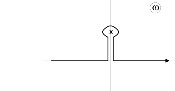
Fig. 1: The contour in the integral over the Euclidean energy variable, $\omega$, encircling a positive-energy valence orbit.

In addition to the valence pole, located on the imaginary Euclidean energy axis in the vicinity of 0, there are many other poles in the complex-energy plane. This feature is present in nonlocal models, and also in certain local models, e.g. those with the proper-time regularization [64]. Fortunately, for the chosen regulators (3) the other poles lie far away from the origin on the scale $\mathchar 3\relax$, hence they do not interfere with the valence orbit, and the deformation of the $\omega$-integration contour is well-defined.

The pole defined by Eq. (23) occurs at an imaginary $\omega$ and therefore at a negative $\omega^{2}$. The determination of the valence orbit requires therefore an analytic continuation of the regulator to negative arguments because $-e_{{\rm val}}^{2}+\vec{k}^{2}$ can become negative for low-enough $\vec{k}^{2}$. Such analytic continuation causes no problem for the forms (3) of the regulator, but it prevents us from using the regulator derived from the instanton model of the vacuum [14], because the latter has a branching point at $k^{2}=0$. The analytic continuation is only required for small negative values of $k^{2}=\omega^{2}+\vec{k}^{2}$, considerably smaller than the nonlocality scale $\mathchar 3\relax^{2}$. Indeed, $e_{{\rm val}}$ lies within $\pm M$, and, on the average, $k^{2}=-e_{v}^{2}+\vec{k}^{2}$ remains very small relative to $\mathchar 3\relax^{2}.$

2.5 The Euler-Lagrange equations for the soliton

The static meson fields are determined self-consistently by solving the Euler-Lagrange equations derived by minimizing the energy (15) with respect to variations of the fields $S$ and $P$:

$$\frac{S\left(\vec{x}\right)}{G^{2}} = N_{c}{\rm z}_{{\rm val}}\langle{\rm val}|r|\vec{x}\rangle\beta\langle\vec{x}|r|{\rm val}\rangle+\intop_{-\infty}^{\infty}\frac{d\omega}{2\pi}\sum_{\lambda_{\omega}}\frac{\langle\lambda_{\omega}|r|\vec{x}\rangle\beta\langle\vec{x}|r|\lambda_{\omega}\rangle}{i\omega+e_{\lambda}\left(\omega^{2}\right)},$$ (25)

$$\frac{P_{a}\left(\vec{x}\right)}{G^{2}} = N_{c}{\rm z}_{{\rm val}}\langle{\rm val}|r|\vec{x}\rangle i\beta\gamma_{5}\tau_{a}\langle\vec{x}|r|{\rm val}\rangle+\intop_{-\infty}^{\infty}\frac{d\omega}{2\pi}\sum_{\lambda_{\omega}}\frac{\langle\lambda_{\omega}|r|\vec{x}\rangle i\beta\gamma_{5}\tau_{a}\langle\vec{x}|r|\lambda_{\omega}\rangle}{i\omega+e_{\lambda}\left(\omega^{2}\right)},$$

where $\left|{\rm val}\right\rangle$ is the valence orbit, and the residue factor is

$${\rm z}_{{\rm val}}=\left(1-i\left.\frac{de_{{\rm val}}(\omega)}{d\omega}\right|_{\omega=ie_{{\rm val}}}\right)^{-1}.$$ (26)

Because the energies $e_{\lambda}\left(\omega^{2}\right)$ and the wave functions $\left|\lambda_{\omega}\right\rangle$ depend only on $\omega^{2}$, we may symmetrize the integrands with respect to $\omega$ and rewrite the Dirac-sea parts of Eqs. (25) in the manifestly real form

$$\intop_{-\infty}^{\infty}\frac{d\omega}{2\pi}\sum_{\lambda_{\omega}}\frac{e_{\lambda}\left(\omega^{2}\right)\langle\lambda_{\omega}|r|\vec{x}\rangle\beta\langle\vec{x}|r|\lambda_{\omega}\rangle}{\omega^{2}+e_{\lambda}^{2}\left(\omega^{2}\right)},$$ (27)

$$\intop_{-\infty}^{\infty}\frac{d\omega}{2\pi}\sum_{\lambda_{\omega}}\frac{e_{\lambda}\left(\omega^{2}\right)\langle\lambda_{\omega}|r|\vec{x}\rangle i\beta\gamma_{5}\tau_{a}\langle\vec{x}|r|\lambda_{\omega}\rangle}{\omega^{2}+e_{\lambda}^{2}\left(\omega^{2}\right)}.$$

The soliton is calculated iteratively. An initial guess is made for the fields $S$ and $P$. In terms of these, the quark orbits (13) are calculated for different values of $\omega$. The fields $S$ and $P$ are then recalculated using (25), and so on until convergence is reached.

3 The vacuum sector

The vacuum sector of our model, analyzed in Refs. [20, 21, 22], is used to constrain the model parameters, namely the strength of the quark-quark interaction $G$, the cut-off $\mathchar 3\relax$, and the current quark mass $m$. We fit the pion decay constant, $f_{\pi}=93$ MeV, and the pion mass, $m_{\pi}=139$ MeV. This leaves one undetermined parameter, which we choose to be $M$, the vacuum value of the scalar field $S$. Admittedly, it is somewhat abusive to claim that the model depends only on three parameters. It is only true to the extent that the regulator $r_{k}$ is expressed in terms of one parameter, such as the cut-off appearing in (3). The model depends in fact on the shape of the regulator and furthermore, as we have seen in Sect. 2.4, the construction of the valence orbit relies on the possibility of the analytic continuation of the regulator to (small) negative momenta $k^{2}$.

For smooth regulators it is found that quantities such as masses, $f_{\pi}$, or $m_{\pi}$, which would diverge logarithmically with the cut-off, do not depend very much on its shape. When one of these quantities is fixed, $f_{\pi}$ for example, the masses of mesons and of solitons do not depend very much on the form of the regulator. However, quantities, such as the quark condensate, which diverge quadratically with the cut-off, are more sensitive to the shape of $r_{k}$ and different values are obtained with different shapes even when $f_{\pi}$ is kept fixed [65]. This can be seen from Table 1. In the whole range of values $300<M<600$, the cut-off of the Gaussian regulator remains $1.06$ times larger than the cut-off of the monopole regulator, within 1% accuracy. The two regulators have the same low-$k$ behavior, therefore the shape dependence is roughly a 6% effect on quantities such as $f_{\pi}$ or $m_{\pi}$.

One may rephrase the above statements as follows: for any given $M$ we fit $\mathchar 3\relax$ for each regulator (Gaussian and monopole) in such a way that $f_{\pi}$ is fixed to 93 MeV. Then, the regulators (3), each with its own $\mathchar 3\relax$, are very similar functions of the $k^{2}$ variable up to $k^{2}\simeq 7\;{\rm fm}^{-2}$ when $M=300$ MeV, and $k^{2}\simeq 3.5\;{\rm fm}^{-2}$ when $M=600$ MeV. Therefore, the quantities dominated by low values of $k^{2}$ depend only weakly on the regulator.

Regulator	$M$	$\mathchar 3\relax$	$m$	$\langle{\frac{1}{2}}\bar{q}q\rangle^{1/3}$	$1/G$	$\langle{\frac{\alpha_{s}}{\pi}}G_{\mu\nu}^{a}G^{\mu\nu}_{a}\rangle^{1/4}$
	[MeV]	[MeV]	[MeV]	[MeV]	[MeV]	[MeV]
	300	760	7.62	$-222$	182	327
	350	627	10.4	$-200$	140	310
Gaussian	400	543	13.2	$-185$	113	298
	450	484	15.9	$-174$	94	287
	600	380	24.2	$-151$	61	268
	300	718	3.96	$-276$	204	347
	350	590	5.24	$-252$	159	334
monopole	400	509	6.44	$-235$	130	323
	450	452	7.56	$-223$	110	315
	600	352	10.5	$-200$	74	294

Table 1: The vacuum properties for the two regulators considered, and for various values of the constituent quark mass $M$. For each case the values of $F_{\pi}$ and $m_{\pi}$ have been fixed to their physical values.

3.1 The quark propagator in the vacuum

In the vacuum sector, the fields acquire the values $S=M$ and $P=0$, and the inverse quark propagator is diagonal in momentum space. In the chiral limit $m\rightarrow 0$, it is equal to $k_{\mu}\gamma_{\mu}+r_{k}^{2}M$. Poles of the quark propagator occur when $k^{2}=-M^{2}r^{4}\left(k^{2}\right)$, where $k^{2}=\omega^{2}+\vec{k}^{2}$. The solution of this equation can be written in the form $k^{2}=-M_{q}^{2}$, where $M_{q}$ satisfies the equation:

$$M_{q}^{2}=M^{2}r^{4}\left(-M_{q}^{2}\right).$$ (28)

This non-linear equation for $M_{q}^{2}$ has, in general, solutions which are scattered in the complex $k^{2}$ (or $M_{q}^{2}$) plane. If $M/\mathchar 3\relax$ is small enough, a solution occurs on the real axis of the $M_{q}^{2}$ plane and such a pole represents an on-shell free quark with a mass equal to $M_{q}$, which we call the vacuum on-shell quark mass. This on-shell quark mass $M_{q}$ can be considerably larger than $M$, which we call the constituent quark mass. As we shall see in Sect. 4, it is the on-shell quark mass $M_{q}$, and not the constituent quark mass $M$, which determines the stability of the soliton (see the discussion of Fig. 2). When the energy (24) is greater than $N_{c}M_{q}$, the soliton is not formed, which means that the Euler-Lagrange equations (25) do not have a localized stationary solution. The soliton can thus be viewed as a bound state. The stability of the soliton is discussed at the end of Sect. 4.

3.2 The gap equation and the condensates

When discussing the model in the vacuum sector, it is much simpler to use the Lorentz-invariant form (5) of the action. In the vacuum sector, a translationally invariant stationary point of the action exists with $S=M$, $P_{a}=0$, where $M$ is the solution of the equation:

$$\frac{1}{G^{2}}=4N_{c}N_{f}\intop\frac{d_{4}k}{\left(2\pi\right)^{4}}\;\frac{r_{k}^{4}}{k^{2}+\left(m+r_{k}^{2}M\right)^{2}}\;.$$ (29)

Equation (29) is traditionally called the “gap equation”. It is the Euler-Lagrange equation expressed for a translationally-invariant system (without valence quarks). For a given current quark mass $m$ (which is determined by fitting $m_{\pi}$), the gap equation (29) relates $M$ to the interaction strength $G$. In this work we use it in order to eliminate the parameter $G$ in favor of $M$.

The quark condensate $\left\langle\bar{q}q\right\rangle=\left\langle\bar{u}u+\bar{d}d\right\rangle$ can be obtained from the action (5). In the chiral limit it is equal to

$$\left\langle\bar{q}q\right\rangle=\frac{1}{\mathchar 10\relax}\left.\frac{\partial I}{\partial m}\right|_{m=0}=4N_{c}N_{f}\intop\frac{d_{4}k}{\left(2\pi\right)^{4}}\;\frac{r_{k}^{2}}{k^{2}+\left(r_{k}^{2}M\right)^{2}}.$$ (30)

In the instanton model of the QCD vacuum the gluon condensate can be expressed in terms of the constituent quark mass and the four-fermion coupling constant [66]:

$$\left\langle\frac{\alpha_{s}}{\pi}G_{\mu\nu}^{a}G_{a}^{\mu\nu}\right\rangle=32N_{c}\intop\frac{d_{4}k}{(2\pi)^{4}}\frac{r_{k}^{4}M^{2}}{k^{2}+\left(r_{k}^{2}M\right)^{2}}=\frac{8M^{2}}{N_{f}G^{2}}.$$ (31)

The numerical values are listed in Table 1. The estimate for the gluon condensate inferred from the QCD sum rules [67, 68] is $\left\langle\frac{\alpha_{s}}{\pi}G^{2}\right\rangle^{1/4}=360\pm 20\,{\rm MeV}$, while Ref. [69] gives the value $386\pm 10\,{\rm MeV}$. These estimates, when compared to the numbers in Table 1, favor lower values of $M$ in our model.

3.3 The pion mass and the pion decay constant

The inverse pion propagator $K_{P}^{-1}(x,y)$ in the vacuum can be deduced from the action (5):

$$\left\langle xa\left|K_{P}^{-1}\right|yb\right\rangle=\frac{\delta^{2}I\left(S,P\right)}{\delta P_{a}\left(x\right)\delta P_{b}\left(y\right)}\;.$$ (32)

Explicit expressions for the meson propagators, $f_{\pi}$, and $m_{\pi}$, calculated with the present model, can be found in Refs. [14, 20, 21, 22, 62] and we shall not reproduce them here. We only specify the expressions used to determine the model parameters. The pion propagator is diagonal in momentum and flavor space: $\left\langle qa\left|K_{P}^{-1}\right|q^{\prime}b\right\rangle=\delta_{ab}\delta_{qq^{\prime}}K_{P}^{-1}\left(q^{2}\right)$. To lowest order in $q^{2}$ and $m$ it acquires the form

$$K_{P}^{-1}\left(q^{2}\right)=Z_{\pi}\left(q^{2}+m_{\pi}^{2}\right),$$ (33)

where the inverse residue of the pion pole is

$$Z_{\pi}=2N_{c}N_{f}\;f\left(M\right)$$ (34)

and where the function $f\left(M\right)$ is

$$f\left(M\right)=\intop\frac{d_{4}k}{\left(2\pi\right)^{4}}\frac{r_{k}^{4}-k^{2}r_{k}^{2}\frac{dr_{k}^{2}}{dk^{2}}+k^{4}\left(\frac{dr_{k}^{2}}{dk^{2}}\right)^{2}}{\left(k^{2}+r_{k}^{4}M^{2}\right)^{2}}\;.$$ (35)

The pion decay constant, $f_{\pi}$, is then given by the expression [14, 20, 21]

$$f_{\pi}^{2}=Z_{\pi}M^{2}=2N_{c}N_{f}M^{2}\;f\left(M\right),$$ (36)

and the pion mass equals to [14, 20, 21]

$$m_{\pi}^{2}=\frac{2m}{M\;f\left(M\right)}g^{\prime}\left(M\right),\;\;\;\;g^{\prime}\left(M\right)=\intop\frac{d_{4}k}{\left(2\pi\right)^{4}}\;\frac{r_{k}^{2}}{k^{2}+r_{k}^{4}M^{2}}.$$ (37)

From Eq. (30) we can see that, in the chiral limit, the quark condensate is $\left\langle\bar{q}q\right\rangle=-4N_{c}N_{f}Mg^{\prime}\left(M\right)$. Using (36), Eq. (37) can be cast into the form

$$m_{\pi}^{2}=-\frac{m\left\langle\bar{q}q\right\rangle}{f_{\pi}^{2}\;},$$ (38)

which is the Gell-Mann–Oakes–Renner relation, requested by the constraints of the chiral symmetry.

The model parameters $M$, $\mathchar 3\relax$, $m$, and $G$ are listed in Table 1. We notice that when $M$ increases, the cut-off $\mathchar 3\relax$ decreases. This occurs because the pion decay constant is kept fixed at the value $f_{\pi}=93$ MeV. For large $\mathchar 3\relax$, the quark condensate increases linearly with $M$ and decreases quadratically with $\mathchar 3\relax$. The net result is a slow decreases with $M$. The coupling constant $G$ of the attractive quark-quark interaction increases with $M$. This is why solitons are bound only when $M$ is large enough, as discussed in Sect. 4. At large values, $M>450\;{\rm MeV}$, the cut-off becomes embarrassingly small as compared to the other scales in the problem. The error of taking the leading expressions in $m$ extends from 2 % at $M=300$ MeV to 10 % at $M=600$ MeV. This estimate is based on the difference of the integrals (30), (31), (35) and (37) in the chiral limit with $m$ from Table 1.

Fig. 2: The energy of the soliton (bold solid line), $N_{c}$ times the free-space on-shell quark mass (thin solid line), and the valence contribution to the soliton energy (dashed line), plotted as functions of the parameter $M$. The dotted line shows the cut-off parameter, $\mathchar 3\relax$, fitted to obtain $f_{\pi}=93$ MeV. All quantities in MeV. The Gaussian regulator is used.

4 Properties of the soliton

The soliton is calculated self-consistently by solving iteratively the Euler-Lagrange equations (25) for the meson fields and the Dirac equation for the quark orbits (13), as described in Sect. 2. The convergence is fast except for very low values of $M$. Because of the presence of the regulator which cuts off very high momenta, it is not necessary to use a very large basis as in similar calculations in local models. We have performed the calculation with two shapes (3) of the regulator, Gaussian and the monopole (3). The soliton properties are sensitive to low values of $k^{2}$, such that, according to the discussion in the beginning of Sect. 3, the results depend very weakly on the shape of the regulator [70] (see Table 2) .

Fig. 3: Self consistently determined fields for various values of $M$, plotted as functions of the radial coordinate $x$. The Gaussian regulator is used.

Figure 2 shows the energy of the soliton obtained with the Gaussian regulator. All quantities are plotted as a function of the constituent quark mass, $M$. The energy of the soliton is a slightly increasing function of $M$ while the energy of the valence orbit flattens out. The soliton energy varies from about 1100 to 1250 MeV when $M$ increases from 300 MeV to 450 MeV. These seem to be reasonable values for a soliton which is to describe the nucleon, because the energy is expected to decrease by about 200 MeV when the center-of-mass energy is subtracted in a suitable projection method [48, 49, 50, 51, 52].

The curve labelled $3M_{q}$ gives $N_{c}=3$ times the value of the on-shell quark mass $M_{q}$ in the vacuum. It is a solution of Eq. (28). The curve terminates when $M\simeq 309$ MeV, or, more precisely, when $\frac{M}{\mathchar 3\relax}\simeq\sqrt{\frac{1}{2e}}=0.43$. (The exact value depends on the shape of the regulator and on $m$.) Indeed, for larger values of $\frac{M}{\mathchar 3\relax}$, Eq. (28) no longer has real solutions and the “on-shell” quark mass wanders off into the complex plane. This has been claimed to be related to quark confinement [6, 18], although the nature of this relation is far from clear. The on shell valence orbit in the background hedgehog field, defined by Eq. (23), exists even when the model parameters prevent the occurrence of an on-shell quark pole in the vacuum background field.

A bound state of quarks occurs when the soliton energy $E$ is lower than the energy of $N_{c}=3$ on-shell quarks, that is, when $E<N_{c}M_{q}$. Figure 2 shows that a bound state of quarks only occurs when $M$ exceeds a critical value of 276 MeV (i.e. when the coupling constant $G>4.12/\mathchar 3\relax$ ). Beyond the critical value of $M$ where $M_{q}$ becomes complex, a stable solution continues to exist. A very similar behavior is found for the monopole regulator.

Fig. 4: Effective squared quark mass in the soliton plotted as a function of the radial coordinate $x$. The Gaussian regulator is used.

Figure 3 shows the radial shapes of the hedgehog chiral fields $S\left(x\right)$ and $P\left(x\right)$ in units of $M$. They are the solutions of the Euler-Lagrange equations (25). We can see that, in the reasonable range $350\;{\rm MeV}<M<450\;{\rm MeV}$, the chiral field deviates significantly from the chiral circle. Only at excessively high values, $M>600$ MeV, does the chiral field remain close to the chiral circle. This is a new dynamical result. In previous soliton calculations, which used the Nambu Jona-Lasinio model with proper-time or Pauli-Villars regularizations [12, 39], the soliton was found to be unstable (the energy was unbounded from below) unless the fields were artificially constrained to the chiral circle [40, 41]. Our model is free from this restriction. In our soliton, the self-consistent pion field is considerably smaller, as compared to previous calculations. In a sense, it is midway between the Skyrmion (where the chiral field is on the chiral circle) and the Friedberg-Lee soliton [71, 72] (where the pion field is zero). Deviations from the chiral circle are further illustrated in Fig. 4 which shows the values of $S^{2}\left(x\right)+P_{a}^{2}\left(x\right)$ in units of $M^{2}$. The curve would remain constant and equal to 1 if the fields remained on the chiral circle. Another way to phrase the behavior displayed in Fig. 4 is to say that the chiral symmetry is partially restored in the center of the soliton.

Fig. 5: The upper ($u$) and lower ($v$) quark components for the valence orbit for various values of $M$, plotted as functions of the radial coordinate $x$. The Gaussian regulator is used.

Figure 5 shows the upper ($u$) and lower ($v$) quark components for the valence orbit for various values of $M$. We note that the solution shrinks as $M$ is increased, however, beyond $M\simeq 450$ MeV the effect saturates.

Fig. 6: The energy per quark for the soliton with three valence quarks (bold solid line), one valence quark (dashed line), and two valence quarks (dashed-dotted line), plotted as functions of the parameter $M$. The thin solid line shows free-space on-shell quark mass $M_{q}$. All quantities in MeV. The Gaussian regulator is used.

Figure 6 illustrates the stability of the soliton, composed of 3 quarks, with respect to its fragmentation into solitons formed with 1 or 2 quarks. Due to the lack of confinement, such solutions formally exist in the model. The solid line, labelled $\frac{1}{3}E_{sol}\left(3q\right)$, shows the soliton energy per quark. The dashed and dot-dashed lines show the energy of the single-quark and two-quark soliton, respectively. The curve labelled $M_{q}$ is the on-shell mass of the quark in the vacuum. We conclude from Fig. 6 that the 3-quark soliton is stable against the breakup into solitons with a lower number of quarks. Similar results have been found in the linear sigma model with valence quarks [73]. Note that the Pauli principle prevents placing more than $N_{c}=3$ quarks into the $0^{+}$ valence orbit.

Regulator	$M$	$e_{{\rm val}}$	$E_{{\rm sea}}$	$E_{{\rm mes}}$	$E_{{\rm sol}}$
	[MeV]	[MeV]	[MeV]	[MeV]	[MeV]
	300	298	2420	$-2227$	1088
	350	285	1773	$-1450$	1180
Gaussian	400	279	1494	$-1102$	1228
	450	275	1339	$-905$	1260
	600	272	1117	$-619$	1313
	300	289	3008	$-2790$	1084
	350	275	2201	$-1850$	1176
monopole	400	266	1835	$-1407$	1227
	450	260	1628	$-1147$	1261
	600	248	1332	$-753$	1321

Table 2: Contributions to the soliton energy calculated with various regulators.

5 Noether currents

The Noether currents in nonlocal models acquire extra contributions due to the momentum-dependent regulator. As mentioned in the introduction, the transverse parts of Noether currents are not fixed by current conservation and their choice is not unique. Any prescription becomes an element of the model building. The problem of ambiguous transverse currents has been known for a long time in connection with meson-exchange currents [20, 21]. An elegant way of gauging the nonlocal model is to use path-ordered $P$-exponents, and we choose this technique to construct the Noether currents.

The details are shown in Appendices A-B. In this section we make some general remarks:

• The ambiguity in the choice of Noether currents is attributed to the freedom of choosing the path in the $P$-exponent.

• The Noether currents associated to symmetries are conserved.

• The properties of solitons involving zero-momentum probes, such as the baryon number and $g_{A}$, do not depend on the chosen path in the $P$-exponent. They are thus defined unambiguously.

• Soliton radii, magnetic moments, form factors, do depend on the path, and hence they are not uniquely determined. We find, however, that the path-dependence is weak in the weak-nonlocality limit, i.e. in the case where the soliton scales are much smaller than the nonlocality scale, $\mathchar 3\relax.$ This is the case for sufficiently large solitons.

Using a straight-line path in the $P$-exponent, we derive in App. C the following form for the nonlocal contributions to Noether currents:

$$j_{\mu a}^{{\rm NL,straight}}\left(\vec{z}\right) = -\intop\frac{d\omega}{2\pi}\sum_{\lambda_{\omega}}\intop d_{3}x\intop d_{3}y\intop_{0}^{1}d\alpha\,\delta(\vec{z}-\vec{x}-\alpha\left(\vec{y}-\vec{x}\right))\times$$ (39)

$$\frac{\langle\lambda_{\omega}|\vec{x}\rangle\langle\vec{x}|r_{\mu}(\omega)|\vec{y}\rangle\langle\vec{y}|\lambda_{a}\beta\mathchar 8\relax r(\omega)|\lambda_{\omega}\rangle}{i\omega+e_{\lambda}\left(\omega\right)}+h.c.,$$

where $\lambda_{a}$ stands for $1/N_{c},\tau_{a}/2,$ or $\gamma_{5}\tau_{a}/2$ in the case of the baryon, isospin, or axial currents, respectively. The parameter $\alpha$ describes the straight-line integration path. The space integrations reflect the nonlocality. The form (39) looks somewhat complicated. However, moments of currents ($g_{A}$, radii, or magnetic moments) are very easily evaluated because, for those cases, the $\alpha$ integration and one space integration can be performed trivially (see App. E for examples) leaving only one space integral, as in the local contributions.

A simpler expression for the Noether currents can be derived in the weak-nonlocality limit [13]. As shown in App. D, we have:

$$j_{\mu a}^{{\rm NL,weak}}\left(\vec{z}\right)=-\intop\frac{d\omega}{2\pi}\sum_{\lambda_{\omega}}\frac{\langle\lambda_{\omega}|\vec{z}\rangle\langle\vec{z}|r_{\mu}(\omega)\lambda_{a}\beta\mathchar 8\relax r(\omega)|\lambda_{\omega}\rangle}{i\omega+e_{\lambda}\left(\omega\right)}+h.c.$$ (40)

In the calculation of observables, we single out the valence and Dirac-sea parts in Eqs. (39,40) in the usual way, as shown in App. E.

6 Observables

As is well known, the nucleon quantum numbers (spin, flavor) need to be projected out of the hedgehog soliton in order to calculate observables. In the large-$N_{c}$ limit this can be achieved by cranking [57, 74]. The observables fall into two categories, according to whether they are dynamically-independent or dynamically-dependent on cranking. The former ones include $g_{A}$, isoscalar-electric, and isovector magnetic properties, while the latter ones include isovector electric and isoscalar magnetic properties. Observables which are dynamically-independent of cranking are simpler to evaluate, since they involve only the expectation value in the hedgehog state. Technically, they lead to single spectral sums over the quark orbits. Quantities which are dynamically-dependent on cranking involve double spectral sums, and they are difficult to evaluate even in local models [12, 39]. The presence of nonlocality adds extra difficulties: an integration over the energy variable, and the appearance of nonlocal contributions. Because of these difficulties, and since the aim in this paper is primarily to develop a consistent approach to calculate observables in the presence of nonlocal regulators, we restrict our calculations to the cranking-independent observables.

6.1 The isoscalar electric radius

Fig. 7: Various contributions to the baryon density (multiplied by $4\pi x^{2}$) for $M=350$ MeV and the Gaussian regulator, plotted as functions of the radial coordinate $x$: the local (solid bold line) and nonlocal (solid thin line) valence contributions, and the local (bold dashed line) and nonlocal (dashed thin curve) sea contributions. The sea contributions are multiplied by a factor of 100.

The results for the mean squared isoscalar electric radius, calculated with the help of the formulas given in App. E.1, are displayed in Table 3 for various values of $M$. The local contribution and different nonlocal contributions (see App. E.1 for their meaning) labeled NL(A), NL(B) and NL(C), are listed separately for the valence orbit and for the Dirac sea. As discussed in the previous section, the radius depends on the chosen path in the $P$-exponent, and the result is not unique. We give the results for a straight line prescription and for the weak-nonlocality approximation.

The expressions for the nonlocal terms contain a derivative of the regulator which produces a factor $1/(2\mathchar 3\relax^{2})$, which suppresses the nonlocal contribution, as compared to the local one. Since $\mathchar 3\relax$ decreases with increasing $M$, the nonlocal terms become more and more important for larger $M$ and the difference between the two prescriptions of evaluating the Noether currents increases. The difference is reasonably small for the physically relevant values of $M$. The soliton is weakly bound for the values of $M$ just above the threshold and hence very large. Its size decreases and reaches the minimum around $M=450$ MeV. Above this value, the radius starts increasing again. This is due to the fact that $\mathchar 3\relax$ is very small and the size becomes proportional to the inverse $\mathchar 3\relax$.

The nonlocal contribution from the valence orbit considerably reduces the isoscalar electric radius, up to 20% for low values of $M$. This is consistent with the fact that the inverse residue, ${\rm z}_{{\rm val}}$, and hence the integrated local density, is greater than 1. The corresponding nonlocal density is negative for all $|\vec{x}|$ (see Fig. 7). We can also see that the weak-nonlocality limit works better for lower values of $M$. This is natural, because the weak-nonlocality limit may be viewed as the leading-order term in an expansion in powers of $1/(R\mathchar 3\relax)$, where $R$ describes the soliton size. This is why the $B$ terms, carrying more derivatives of $r$, are much smaller than the $A$ and $C$ terms. By the same argument, in the weak-nonlocality limit $A=C$. We note finally that our numbers for $\langle r^{2}\rangle_{\rm baryon}$ are larger than the experimental value of 0.62 fm².

Different contributions to the baryon (isoscalar electric) density are displayed in Fig. 7. As a numerical check we have verified that the sum of the valence contributions integrates to 1, while the sum of the sea contributions integrates to 0.

		$M$ [MeV]
$\langle r^{2}\rangle_{{\rm baryon}}$		300	350	400	450	600
val	L	2.209	1.270	1.057	0.991	1.062
	NL (A)	$-0.446$	$-0.228$	$-0.188$	$-0.192$	$-0.328$
	NL (B)	$-0.039$	$-0.039$	$-0.040$	$-0.041$	$-0.061$
	NL (C)	$-0.435$	$-0.194$	$-0.119$	$-0.074$	0.021
	straight line	1.761	1.052	0.897	0.852	0.898
	weak NL	1.773	1.075	0.937	0.917	1.083
sea	L	0.0050	0.0070	0.0080	0.0080	0.0075
	NL (A)	0.0005	0.0012	0.0020	0.0022	0.0030
	NL (B)	0.0001	0.0001	0.0002	0.0002	0.0003
	NL (C)	0.0003	0.0010	0.0015	0.0018	0.0026
total	straight line	1.766	1.060	0.907	0.862	0.909
	weak NL	1.778	1.083	0.947	0.927	1.094

Table 3: Various contributions to the isoscalar electric mean square radius. L denotes the local contribution and NL(A,B,C) different nonlocal contributions defined in App. E.1. The total result is displayed for the straight path and in the weak-nonlocality approximation. The Gaussian regulator is used.

6.2 $g_{A}$

The results for $g_{A}$, evaluated with the expressions given in App. E.2, are displayed in Table 4. The sea contribution remains small for all values of $M$. The nonlocal terms increase with increasing $M$, as expected, yielding, together with the local piece, almost a constant value of $g_{A}$ over a wide range of $M$. The values, ranging between 1.1 and 1.15, are somewhat smaller than the experimental value of 1.26.

	$M$ [MeV]
$g_{A}$	300	350	400	450	600
val, L	1.047	0.922	0.861	0.819	0.737
val, NL	0.022	0.069	0.119	0.170	0.309
sea, L	0.050	0.067	0.064	0.058	0.037
sea, NL	0.032	0.053	0.062	0.065	0.062
total	1.151	1.112	1.106	1.112	1.146

Table 4: Different contributions to $g_{A}$ calculated from the current. L and NL denote the local and nonlocal contributions, respectively. The Gaussian regulator is used.

6.3 Isovector magnetic moments and radii

The results for the isovector magnetic moment, evaluated with the expressions given in App. E.3, are shown in Table 5. As in the case of $g_{A}$, the nonlocal terms increase with increasing $M$, and the total value is almost constant over a wide range of $M$. The values are lower than the experimental value 4.71.

		$M$ [MeV]
$\mu_{I=1}$		300	350	400	450	600
val	L	2.910	2.519	2.339	2.245	2.174
	NL	0.097	0.212	0.319	0.420	0.673
sea	L	0.293	0.379	0.386	0.372	0.305
	NL	0.122	0.198	0.238	0.262	0.289
total		3.422	3.307	3.282	3.299	3.442

Table 5: Contributions to the isovector magnetic moment, in units of the nuclear magneton. L and NL denote the local and nonlocal contributions, respectively. The Gaussian regulator is used.

In Table 6 we list different contributions to the squared isovector magnetic radius, evaluated with the expressions given in App. E.3. This quantity depends on the prescription for the Noether current, but the difference between the straight-line path method and the weak-nonlocality approximation is even smaller than in the case of the baryon radius (see Table 3). The sea contribution is substantially larger than in the isoscalar electric case. The numbers are much larger than the experimental value of 0.77 fm².

		$M$ [MeV]
$\langle r^{2}\rangle_{M,I=1}$		300	350	400	450	600
val	L	2.498	1.288	1.043	1.001	1.285
	NL	0.073	0.112	0.153	0.196	0.334
sea	L	0.378	0.424	0.421	0.405	0.343
	NL	0.137	0.187	0.220	0.243	0.276
total	straight line	3.087	2.011	1.838	1.846	2.238
	weak L	3.087	2.011	1.837	1.844	2.226

Table 6: Various contributions to the isovector magnetic mean square radius. L and NL denote the local and nonlocal contributions, respectively. The total result is displayed for the straight path and in the weak-nonlocality approximation. The Gaussian regulator is used.

To summarize the results for the observables, we note that the soliton, at the present mean-field treatment, is too large. This leaves room for the inclusion of other effects. One important effect comes from the center-of mass corrections which reduce both the mass and the mean square radii. The fields which describe the soliton break translational symmetry. The center of mass of the system is not at rest and it makes a spurious contribution both to the energy and to the mean square radii (more generally, to the form factors). This spurious contribution should be subtracted from the calculated values. The subtraction is a next-to-leading-order correction in $N_{c}$. A rough estimate can be obtained from an oscillator model. If $N_{c}$ particles of mass $m$ move in the $1s$ state of a harmonic oscillator of frequency $\hbar\omega$, the center of mass of the system is also in a $1s$ state and it contributes $\frac{3}{4}\hbar\omega=\left\langle P^{2}\right\rangle/2N_{c}m$ to the energy. Thus, we can correct the soliton energies by subtracting $\left\langle P^{2}\right\rangle/2E_{sol}$ from the calculated energy. Furthermore, in the oscillator model, the center of mass contributes a fraction $\frac{1}{N_{c}}$ of the mean square radius, such that one corrects the mean square radius by multiplying the calculated value by a factor equal to $\left(1-\frac{1}{N_{c}}\right)$. These corrections to the soliton mass and the isoscalar electric radius may bring the calculated values close to the experimental ones [38]. To some extent, the too large soliton may also reflect the lack of confinement of the model, or some other omitted dynamical factor, e.g. vector interactions [34, 55]. Although the chiral field is sufficiently strong to bind the quarks, additional forces may reduce the soliton size.

The problem with too low values of $g_{A}$ and of the isovector magnetic moment may be resolved by rotational $1/N_{c}$ corrections, as found in soliton calculations which use proper-time or Pauli-Villars regularizations [53, 54]. The rotational corrections produce a factor lying between 1 and $(N_{c}+2)/N_{c}$, which brings the calculated values closer to the experimental data. This problem requires a further study.

6.4 Calculations with chiral fields constrained to the chiral circle

In chiral quark models the soliton properties have so far only been calculated with the sigma and pion fields constrained to lie on the chiral circle [12, 39]. Although no clear physical ground for such a constraint can be seen in the derivations of effective quark models, it is nonetheless interesting to study its effect in our model.

Fig. 8: The energy of the soliton [in MeV] (bold lines), the three free-space quark mass (solid line) and the valence contribution to the soliton energy (thin lines) plotted as functions of $M$. Solid lines correspond to the unconstrained calculation (same as in Fig. 2), dashed lines to the calculation with the chiral-circle constraint, dashed-dotted to the calculation using proper time regularization, also with the chiral-circle constraint. In the latter case the energy of three free quarks is marked by $3M$. The parameters of all models are fitted to obtain $f_{\pi}=93$ MeV.

Fig. 8 shows the soliton energy of the constrained calculation as a function of $M$. The constrained energy is 150 MeV higher than the energy of our solution at smaller values of $M$ and stays some 70 MeV higher even in the region where the unconstrained chiral fields come closer to the chiral circle. From Fig. 3 it is clear that in the unconstrained calculation it is energetically favorable to increase more the magnitude of the sigma field than the pion field. Contrary to the unconstrained calculation where the soliton energy at the threshold continues smoothly from the curve representing the energy of three free quarks, the energy of the constrained soliton starts abruptly at $M=298$ MeV and in a small region of $M$ just above the threshold stays above the $3M_{q}$ curve. Such an energetic instability, absent in the unconstrained nonlocal model, is in fact common to several chiral models [75, 76]; in particular, in the local model with the proper time regularization one finds a self-consistent solution for $338\;{\rm MeV}<M<412\;{\rm MeV}$ even though the soliton is energetically not stable in this region (see the dashed-dotted lines in Fig. 8).

The observables calculated in the constrained calculations are displayed in Table 7. The differences to the unconstrained results presented in Tables 3–6 can be explained by two effects: due to a deeper effective potential in (13) the valence orbits shrinks thus yielding a smaller valence contribution to the magnetic moment and the two radii. On the other hand, due to the stronger chiral fields, the sea contribution to all quantities becomes more important and partially cancels the decreased valence contribution.

		$M$ [MeV]
		300	350	400	450	600
energy	$e_{\mathrm{val}}$	327	287	279	276	275
[MeV]	total	1249	1309	1336	1354	1387
$\langle r^{2}\rangle_{{\rm baryon}}$	valence	1.190	0.711	0.667	0.677	0.798
[fm2]	total	1.201	0.725	0.684	0.694	0.813
$g_{A}$	valence	1.150	0.978	0.982	1.003	1.087
	total	1.205	1.079	1.084	1.100	1.164
$\mu_{I=1}$	valence	2.444	2.232	2.259	2.334	2.647
	total	3.223	3.065	3.088	3.146	3.388
$\langle r^{2}\rangle_{M,I=1}$	valence	1.692	0.873	0.844	0.930	1.465
[fm2]	total	2.437	1.621	1.599	1.681	2.173

Table 7: Various observables (see Tables 2–6) obtained in the calculation with the chiral-circle constraint. “Valence” stands for the sum of the local and nonlocal contributions, the radii are calculated with the straight line prescription.

7 Conclusions

In this paper we have shown that a soliton, i.e. a bound state of $N_{c}=3$ quarks, is formed in a chiral quark model with nonlocal regulators. We have demonstrated its energetic stability and investigated its basic properties. Moreover, we have developed a scheme for quantizing the baryon number of the soliton, as well as for calculating observables. The construction of Noether currents has been accomplished through the use of straight line path-ordered $P$-exponents. This construction is general and applicable to any model with nonlocal separable four-fermion interactions.

We have shown that the nonlocal regularization, which is somewhat more and yet not prohibitively complicated, has several attractive features compared to the chiral quark models which use local regularizations, such as the Pauli-Villars or the Schwinger proper-time method. We have found that the pion field is considerably reduced compared to the local models which require the chiral field to remain on the chiral circle. The soliton is found to have properties which make it suitable for the description of the nucleon and for application of further corrections, such as projection [48, 49, 50, 51, 52], or the inclusion of $1/N_{c}$ corrections [53, 54].

The authors wish to thank Enrique Ruiz Arriola, Michael Birse, Klaus Goeke, Maxim Polyakov, and Nikos Stefanis for many useful discussions and comments.

A The gauged nonlocal model

Consider the gauge transformation of the quark field,

$$q(x)\rightarrow e^{-i\lambda^{a}\phi_{a}(x)}q(x),$$ (A.1)

where $\lambda^{a}=1/N_{c}$ for the baryon current, $\lambda^{a}=\tau^{a}/2$ for the isospin current, and $\lambda^{a}=\gamma_{5}\tau^{a}/2$ for the axial current. We gauge the nonlocal model by using the path-ordered-exponent method described in Refs. [20, 21, 77]. The method is based on the Wilson line integrals ($P$-exponents) defined as

$$W_{A}(x,y)={\cal P}e^{i\intop_{x}^{y}\lambda^{a}A_{a}^{\mu}(s)ds_{\mu}},$$ (A.2)

where ${\cal P}$ denotes a path ordering operator needed for non-abelian gauge transformations, $\lambda^{a}A_{a}^{\mu}$ is the gauge field (in general non-abelian), and $s$ parameterizes an arbitrary path from $x$ to $y$. The operator $W_{A}(x,y)$ is a functional of the gauge fields $A_{a}^{\mu}$ with the following key property: when the gauge field undergoes the gauge transformation

$$D_{\mu}\rightarrow e^{-i\lambda^{a}\phi_{a}}D_{\mu}e^{i\lambda^{a}\phi_{a}},$$ (A.3)

where $D_{\mu}=\partial_{\mu}+i\lambda^{a}A_{a\mu}$, the operator $W_{A}(x,y)$ transforms as

$$W_{A}(x,y)\rightarrow W_{A+\partial\phi}(x,y)=e^{-i\lambda^{a}\phi_{a}\left(x\right)}W_{A}(x,y)e^{i\lambda^{a}\phi_{a}\left(y\right)}.$$ (A.4)

Consider the quark-loop term of the Euclidean action (5),

$$I_{q}=-{\rm Tr}\ln\beta\left(-i\partial_{\mu}\gamma_{\mu}+m+r\,\mathchar 8\relax\,r\right).$$ (A.5)

The gauged action is constructed by making the substitutions

$$\partial_{\mu}\rightarrow D_{\mu},\quad\quad\left\langle x\left|r\right|y\right\rangle\rightarrow\left\langle x\left|r_{A}\right|y\right\rangle=W_{A}\left(x,y\right)\left\langle x\left|r\right|y\right\rangle,$$ (A.6)

and

$$\beta\mathchar 8\relax\rightarrow e^{-i\lambda^{a}\phi_{a}(x)}\beta\mathchar 8\relax e^{i\lambda^{a}\phi_{a}(x)}.$$ (A.7)

In explicit form the gauged action reads

$$I_{q}\left(A\right)=-{\rm Tr}\ln\left(-\beta i\gamma_{\mu}\partial_{\mu}+\beta\gamma_{\mu}\lambda^{a}A_{a\mu}+\beta m+r_{A}\beta\mathchar 8\relax r_{A}\right).$$ (A.8)

Note that, in general, $r_{A}$ and $\beta$ do not commute. In the gauge transformation the action (A.8) transforms to

$$I_{q}\left(A\right) \rightarrow I_{q}\left(A+\partial\phi\right)=$$ (A.9)

$$-{\rm Tr}\ln\left[-i\beta\gamma_{\mu}\partial_{\mu}+\beta\gamma_{\mu}\left(\lambda^{a}A_{a\mu}+\lambda^{a}\phi_{a\mu}+[\lambda^{b}\phi_{b},\lambda^{a}A_{a}^{\mu}]\right)\right.$$

$$\left.+\beta m+r_{A+\partial\phi}e^{-i\lambda^{a}\phi_{a}}\beta\mathchar 8\relax e^{i\lambda^{a}\phi_{a}}r_{A+\partial\phi}\right].$$

Using the property $r_{A+\partial\phi}=e^{-i\lambda^{a}\phi_{a}}r_{A}e^{i\lambda^{a}\phi_{a}}$ we find that

$$I_{q}\left(A+\partial\phi\right) = -{\rm Tr}\ln e^{-i\lambda^{a}\phi_{a}}\beta\left[-i\gamma_{\mu}\partial_{\mu}+\gamma_{\mu}\lambda^{a}A_{a\mu}+e^{i\lambda^{a}\phi_{a}}me^{-i\lambda^{a}\phi_{a}}+\right.$$ (A.10)

$$\left.\beta r_{A}\beta\mathchar 8\relax r_{A}\right]e^{i\lambda^{a}\phi_{a}}.$$

Equation (A.10) shows that, provided $e^{i\lambda^{a}\phi_{a}}\beta me^{-i\lambda^{a}\phi_{a}}=\beta m$ (the case of baryon or isovector symmetries), or in the chiral limit $m=0$, the action is invariant in the gauge transformation,

$$I\left(A+\partial\phi\right)=I\left(A\right),$$ (A.11)

such that the corresponding Noether current, evaluated from the expression

$$j_{\mu}^{a}\left(x\right)=\left.\frac{\delta I\left(A\right)}{\delta A_{\mu}(x)}\right|_{A=0},$$ (A.12)

is conserved:

$$\partial_{\mu}j_{\mu}^{a}\left(x\right)=0.$$ (A.13)

B Explicit construction of Noether currents

The action, expanded to first order in the $A$ field, has the form

$$I^{\left(A\right)} = -{\rm Tr}\frac{1}{-i\partial_{\mu}\beta\gamma_{\mu}+\beta m+r\beta\mathchar 8\relax r}\left(\beta\gamma_{\mu}\lambda^{a}A_{a\mu}+r_{A}^{1}\beta\mathchar 8\relax r+r\beta\mathchar 8\relax r_{A}^{1}\right)$$ (B.1)

$$= -\sum_{\omega,\lambda_{\omega}}\frac{\left\langle\omega,\lambda_{\omega}\left|\beta\gamma_{\mu}\lambda^{a}A_{a\mu}+r_{A}^{1}\beta\mathchar 8\relax r+r\beta\mathchar 8\relax r_{A}^{1}\right|\omega,\lambda_{\omega}\right\rangle}{i\omega+e_{\lambda}\left(\omega\right)},$$

where

$$\left\langle x\left|r_{A}\right|y\right\rangle=\left\langle x\left|r\right|y\right\rangle\left(1+i\intop_{x}^{y}ds_{\mu}\lambda^{a}A_{a\mu}\left(s\right)+...\right)\equiv\left\langle x\left|r\right|y\right\rangle+\left\langle x\left|r_{A}^{1}\right|y\right\rangle+...$$ (B.2)

We can now write, with help of a representation of the $\delta$ function,

$$\left\langle x\left|r_{A}^{1}\right|y\right\rangle=i\intop_{x}^{y}ds_{\mu}\lambda^{a}A_{a\mu}\left(s\right)=i\intop\frac{d_{4}q}{(2\pi)^{4}}\intop_{x}^{y}ds_{\mu}e^{i(z-s)\cdot q}\lambda^{a}A_{a\mu}\left(z\right).$$ (B.3)

The Noether current is obtained from Eq. (A.12), which, according to (B.1,B.3) gives a general expression, valid for any path in the $P$-exponent:

$$j_{\mu a}\left(z\right)\equiv j_{\mu a}^{L}\left(z\right)+j_{\mu a}^{NL}\left(z\right)$$

$$= -\sum_{\omega,\lambda_{\omega}}\frac{\langle\omega,\lambda_{\omega}\left|z\rangle\beta\gamma_{\mu}\lambda_{a}\langle z\right|\omega,\lambda_{\omega}\rangle}{i\omega+e_{\lambda}\left(\omega\right)}-\sum_{\omega,\lambda_{\omega}}i\intop\frac{d_{4}q}{(2\pi)^{4}}\intop d_{4}x\intop d_{4}y\intop_{x}^{y}ds_{\mu}e^{i(z-s)\cdot q}\times$$

$$\frac{\langle\omega,\lambda_{\omega}|x\rangle\langle x|r|y\rangle\langle y|\lambda_{a}\beta\mathchar 8\relax r|\omega,\lambda_{\omega}\rangle+\langle\omega,\lambda_{\omega}|r\beta\mathchar 8\relax\lambda_{a}|x\rangle\langle x|r|y\rangle\langle y|\omega,\lambda_{\omega}\rangle}{i\omega+e_{\lambda}\left(\omega\right)},$$

where $j_{\mu a}^{L}$ and $j_{\mu a}^{NL}$ are the local and nonlocal contributions, respectively. We can now check explicitly the current conservation. With help of the equations of motion, we find

$$\partial_{\mu}j_{\mu a}^{L}\left(z\right) = \sum_{\omega,\lambda_{\omega}}\frac{m\langle\omega,\lambda_{\omega}\left|z\rangle\langle z|[\beta,\lambda_{a}]\right|\omega,\lambda_{\omega}\rangle}{\omega-ie_{\lambda}\left(\omega\right)}-$$

$$\sum_{\omega,\lambda_{\omega}}\frac{\langle\omega,\lambda_{\omega}\left|z\rangle\langle z|\beta\lambda_{a}r\mathchar 8\relax r\right|\omega,\lambda_{\omega}\rangle-\langle\omega,\lambda_{\omega}|\beta r\mathchar 8\relax r\lambda_{a}|z\rangle\langle z|\omega,\lambda_{\omega}\rangle}{\omega-ie_{\lambda}\left(\omega\right)}$$

$$\partial_{\mu}j_{\mu a}^{NL}\left(z\right) = \sum_{\omega,\lambda_{\omega}}\frac{\langle\omega,\lambda_{\omega}\left|z\rangle\langle z|\beta\lambda_{a}r\mathchar 8\relax r\right|\omega,\lambda_{\omega}\rangle-\langle\omega,\lambda_{\omega}|\beta r\mathchar 8\relax r\lambda_{a}|z\rangle\langle z|\omega,\lambda_{\omega}\rangle}{\omega-ie_{\lambda}\left(\omega\right)}$$

$$-\sum_{\omega,\lambda_{\omega}}\frac{\langle\omega,\lambda_{\omega}\left|r|z\rangle\lambda_{a}\beta\mathchar 8\relax(z)\langle z|r\right|\omega,\lambda_{\omega}\rangle-\langle\omega,\lambda_{\omega}|r|z\rangle\beta\mathchar 8\relax(z)\lambda_{a}\langle z|r|\omega,\lambda_{\omega}\rangle}{\omega-ie_{\lambda}\left(\omega\right)}.$$

In the second equation we have used the identity

$$\frac{\partial}{\partial z_{\mu}}i\intop\frac{d_{4}q}{(2\pi)^{4}}\intop_{x}^{y}ds_{\mu}e^{i(z-s)\cdot q} = \intop\frac{d_{4}q}{(2\pi)^{4}}\intop_{x}^{y}d(s\cdot q)e^{i(z-s)\cdot q}=$$

$$i\intop\frac{d_{4}q}{(2\pi)^{4}}(e^{i(z-y)\cdot q}-e^{i(z-x)\cdot q}) = i(\delta(z-y)-\delta(z-x)).$$ (B.7)

Combining the local and nonlocal pieces (B,B) (which are not separately conserved), and using the equations of motion for the $S$ and $P$ fields, Eqs. (25), we find that

$$\partial_{\mu}j_{\mu a}\left(z\right)=-\sum_{\omega,\lambda_{\omega}}\frac{\langle\omega,\lambda_{\omega}|z\rangle[\lambda_{a},\beta m]\langle z|\omega,\lambda_{\omega}\rangle}{\omega-ie_{\lambda}\left(\omega\right)}.$$ (B.8)

This immediately leads to the conservation of baryon and isospin current, and, in the chiral limit of $m=0$, to the conservation of the axial current. Note that the conservation laws are independent of the chosen path in the $P$-exponent.

Quantities involving space integrals of Noether currents (charges, $g_{A}$) also do not depend on the path. Indeed, the integration over $z$ in Eq. (B) leads to

$$\intop\frac{d_{4}q}{(2\pi)^{4}}\delta(q)\intop_{x}^{y}ds_{\mu}e^{-is\cdot q}=\intop_{x}^{y}ds_{\mu}=(y^{\mu}-x^{\mu}).$$ (B.9)

and subsequently, through the use of the identity

$$i\left(y_{\mu}-x_{\mu}\right)\left\langle x\left|r\right|y\right\rangle=\left\langle x\left|r_{\mu}\right|y\right\rangle,$$ (B.10)

to

$$\intop d_{3}z\,j_{\mu a}\left(z\right)=-\intop\frac{d\omega}{2\pi i}\sum_{\lambda_{\omega}}\frac{\langle\lambda_{\omega}\left|(\beta\lambda_{a}\gamma_{\mu}+r_{\mu}\lambda_{a}\beta\mathchar 8\relax r+\beta r\mathchar 8\relax\lambda_{a}r_{\mu})\right|\lambda_{\omega}\rangle}{\omega-ie_{\lambda}\left(\omega\right)}.$$ (B.11)

Note that any reference to the choice of the path has disappeared. Thus, charges, which are obtained from Eq. (B.11) with $\mu=0$, or $g_{A}$, which has $\mu=3$ (cf. Sect. 6.2) are independent of the path, hence are uniquely defined. One may easily generalize this result to any Green’s function in the soliton background for the case where the external legs corresponding to Noether currents have vanishing four-momenta. The proof is straightforward through the use of the identity (B.9).

C Straight-line paths

The expression (B) is not, in general, suitable for calculating observables, since the path is not specified. A popular choice of the path is a straight line [20, 21, 23]:

$$s_{\mu}=x_{\mu}+\alpha\left(y_{\mu}-x_{\mu}\right)\;\;\;\;\;ds_{\mu}=d\alpha\left(y_{\mu}-x_{\mu}\right).$$ (C.1)

Then in Eq. (B) we have

$$\intop\frac{d_{4}q}{(2\pi)^{4}}\intop_{x}^{y}ds_{\mu}e^{i(z-s)\cdot q} = \intop\frac{d_{4}q}{(2\pi)^{4}}\intop_{0}^{1}d\alpha\left(y_{\mu}-x_{\mu}\right)e^{i(z-x-\alpha\left(y-x\right))\cdot q}$$ (C.2)

$$= \intop_{0}^{1}d\alpha\left(y_{\mu}-x_{\mu}\right)\delta(z-x-\alpha\left(y-x\right)),$$ (C.3)

As a result, we find

$$j_{\mu a}^{{\rm NL,straigh}}\left(z\right)=-\sum_{\omega,\lambda_{\omega}}\intop d_{4}x\intop d_{4}y\intop_{0}^{1}d\alpha\,\delta(z-x-\alpha\left(y-x\right))\times$$ (C.4)

$$\frac{\langle\omega,\lambda_{\omega}|x\rangle\langle x|r_{\mu}|y\rangle\langle y|\lambda_{a}\beta\mathchar 8\relax r|\omega,\lambda_{\omega}\rangle+\langle\omega,\lambda_{\omega}|r\beta\mathchar 8\relax\lambda_{a}|x\rangle\langle x|r_{\mu}|y\rangle\langle y|\omega,\lambda_{\omega}\rangle}{i\omega+e_{\lambda}\left(\omega\right)}.$$

Since the fields $\mathchar 8\relax$ are stationary, we can rewrite Eq. (B) in a simpler form

$$j_{\mu a}^{{\rm NL,straigh}}\left(\vec{z}\right)=-\intop\frac{d\omega}{2\pi}\sum_{\lambda_{\omega}}\intop d_{3}x\intop d_{3}y\intop_{0}^{1}d\alpha\,\delta(\vec{z}-\vec{x}-\alpha\left(\vec{y}-\vec{x}\right))\times$$ (C.5)

$$\frac{\langle\lambda_{\omega}|\vec{x}\rangle\langle\vec{x}|r_{\mu}(\omega)|\vec{y}\rangle\langle\vec{y}|\lambda_{a}\beta\mathchar 8\relax r(\omega)|\lambda_{\omega}\rangle+\langle\lambda_{\omega}|r(\omega)\beta\mathchar 8\relax\lambda_{a}|\vec{x}\rangle\langle\vec{x}|r_{\mu}(\omega)|\vec{y}\rangle\langle\vec{y}|\lambda_{\omega}\rangle}{i\omega+e_{\lambda}\left(\omega\right)}.$$

In the second term above, we can interchange $x$ with $y$ and change the integration variable $\alpha\rightarrow 1-\alpha$. This leads to a manifestly Hermitian form,

$$j_{\mu a}^{{\rm NL,straigh}}\left(\vec{z}\right) = -\intop\frac{d\omega}{2\pi}\sum_{\lambda_{\omega}}\intop d_{3}x\intop d_{3}y\intop_{0}^{1}d\alpha\,\delta(\vec{z}-\vec{x}-\alpha\left(\vec{y}-\vec{x}\right))\times$$ (C.6)

$$\frac{\langle\lambda_{\omega}|\vec{x}\rangle\langle\vec{x}|r_{\mu}(\omega)|\vec{y}\rangle\langle\vec{y}|\lambda_{a}\beta\mathchar 8\relax r(\omega)|\lambda_{\omega}\rangle}{i\omega+e_{\lambda}\left(\omega\right)}+h.c.$$

which is used below.

D Weak-nonlocality approximation

For the case where the nonlocality scale $\mathchar 3\relax$ is much larger than other scales in the problem (e.g. the inverse soliton size) we can commute the $r_{\mu}$ operator with $|x\rangle\langle x|$ [13] in Eq. (C.6), thereby obtaining

$$j_{\mu a}^{{\rm NL,weak}}\left(z\right) = -\sum_{\omega,\lambda_{\omega}}\intop d_{4}x\intop d_{4}y\intop_{0}^{1}d\alpha\,\delta(z-x-\alpha\left(y-x\right))\times$$ (D.1)

$$\frac{\langle\omega,\lambda_{\omega}|r_{\mu}|x\rangle\langle x|y\rangle\langle y|\lambda_{a}\beta\mathchar 8\relax r|\omega,\lambda_{\omega}\rangle}{i\omega+e_{\lambda}\left(\omega\right)}+h.c.$$

$$= -\sum_{\omega,\lambda_{\omega}}\frac{\langle\omega,\lambda_{\omega}|r_{\mu}|z\rangle\langle z|\lambda_{a}\beta\mathchar 8\relax r|\omega,\lambda_{\omega}\rangle}{i\omega+e_{\lambda}\left(\omega\right)}+h.c.$$

Finally, commuting $r_{\mu}$ and $|z\rangle\langle z|$ and using the stationarity of $\mathchar 8\relax$ we find

$$j_{\mu a}^{{\rm NL,weak}}\left(\vec{z}\right)=-\intop\frac{d\omega}{2\pi}\sum_{\lambda_{\omega}}\frac{\langle\lambda_{\omega}|\vec{z}\rangle\langle\vec{z}|r_{\mu}(\omega)\lambda_{a}\beta\mathchar 8\relax r(\omega)|\lambda_{\omega}\rangle}{i\omega+e_{\lambda}\left(\omega\right)}+h.c.$$ (D.2)

which is our current in the weak-nonlocality approximation. Note that some arbitrariness is involved here. We could have placed the $|\vec{z}\rangle\langle\vec{z}|$ operator anywhere between $\langle\lambda_{\omega}|$ and $|\lambda_{\omega}\rangle,$ and that would lead to different currents. However, all of these definitions become equal if the scale of the nonlocality is much larger than other scales in the problem, i.e. in the weak-nonlocality limit.

E Evaluation of observables

We calculate observables both with the straight-line prescription and in the weak-nonlocality limit. We work in the Minkowski space, by means of the replacement

$$\gamma_{0}\rightarrow i\beta,\qquad j_{0a}(x)\rightarrow i\rho_{a}(x),$$ (E.1)

with $\rho_{a}$ denoting the Minkowski charge density.

E.1 Baryon mean square radius

The baryon charge mean squared radius equals to

$$\left\langle r^{2}\right\rangle_{B}=\intop d_{3}z\,\,z^{2}\rho_{B}\left(\vec{z}\right),$$ (E.2)

The contribution from the local part of the current is

$$\left\langle r^{2}\right\rangle_{B}^{{\rm L}}=-\frac{1}{N_{c}}\intop\frac{d\omega}{2\pi i}\sum_{\lambda_{\omega}}\intop d_{3}z\frac{\langle\lambda_{\omega}\left|\vec{z}\rangle z^{2}\langle\vec{z}\right|\lambda_{\omega}\rangle}{\omega-ie_{\lambda}\left(\omega\right)}\,,$$ (E.3)

while the nonlocal term gives

$$\left\langle r^{2}\right\rangle_{B}^{{\rm NL,straight}} = -\frac{2}{iN_{c}}\intop d_{3}z\,\,z^{2}\intop\frac{d\omega}{2\pi i}\sum_{\lambda_{\omega}}\intop d_{3}x\intop d_{3}y\intop_{0}^{1}d\alpha\,\times$$ (E.4)

$$\delta(\vec{z}-\vec{x}-\alpha\left(\vec{y}-\vec{x}\right))\frac{\langle\lambda_{\omega}|\vec{x}\rangle\langle\vec{x}|r_{0}(\omega)|\vec{y}\rangle\langle\vec{y}|\beta\mathchar 8\relax r(\omega)|\lambda_{\omega}\rangle}{\omega-ie_{\lambda}\left(\omega\right)}.$$

We can now carry the $\alpha$ integration

$$\intop d_{3}z\,z^{2}\intop_{0}^{1}d\alpha\,\delta(\vec{z}-\vec{x}-\alpha\left(\vec{y}-\vec{x}\right)) = \intop_{0}^{1}d\alpha\,(\vec{x}+\alpha\left(\vec{y}-\vec{x}\right))^{2}=$$

$$\vec{x}^{2}+\vec{x}\cdot(\vec{y}-\vec{x})+\frac{1}{3}\left(\vec{y}-\vec{x}\right)^{2} = \frac{1}{2}\vec{x}^{2}-\frac{1}{6}\left(\vec{y}-\vec{x}\right)^{2}+\frac{1}{2}\vec{y}^{2}$$ (E.5)

to obtain

$$\left\langle r^{2}\right\rangle_{B}^{{\rm NL,straight}} = \frac{1}{2}A+\frac{1}{6}B+\frac{1}{2}C,$$ (E.6)

$$A = -\frac{2}{iN_{c}}\intop\frac{d\omega}{2\pi i}\sum_{\lambda_{\omega}}\intop d_{3}z\,z^{2}\frac{\langle\lambda_{\omega}|r_{0}(\omega)|\vec{x}\rangle\langle\vec{x}|\beta\mathchar 8\relax r(\omega)|\lambda_{\omega}\rangle}{\omega-ie_{\lambda}\left(\omega\right)},$$

$$B = -\frac{2}{iN_{c}}\intop\frac{d\omega}{2\pi i}\sum_{\lambda_{\omega}}\sum_{j=1}^{3}\frac{\langle\lambda_{\omega}|r_{0jj}(\omega)\beta\mathchar 8\relax r(\omega)|\lambda_{\omega}\rangle}{\omega-ie_{\lambda}\left(\omega\right)},$$

$$C = -\frac{2}{iN_{c}}\intop\frac{d\omega}{2\pi i}\sum_{\lambda_{\omega}}\intop d_{3}z\,\,z^{2}\frac{\langle\lambda_{\omega}|\vec{x}\rangle\langle\vec{x}|r_{0}(\omega)\beta\mathchar 8\relax r(\omega)|\lambda_{\omega}\rangle}{\omega-ie_{\lambda}\left(\omega\right)}.$$

In the derivation of $B$ we have used the identity

$$(\vec{x}-\vec{y})^{2}\langle\vec{x}|r_{0}(\omega)|\vec{y}\rangle=-\sum_{j=1}^{3}\langle\vec{x}|r_{0jj}(\omega)|\vec{y}\rangle.$$ (E.7)

The above formulas can be further decomposed into the valence and sea contributions:

$$\left\langle r^{2}\right\rangle_{B}^{{\rm L,val}} = {\rm z}_{{\rm val}}\intop d_{3}z\,\,z^{2}|\langle\vec{z}|{\rm val}\rangle|^{2},$$

$$\left\langle r^{2}\right\rangle_{B}^{{\rm L,sea}} = -\frac{1}{N_{c}}\intop\frac{d\omega}{2\pi}\sum_{\lambda_{\omega}}\frac{e_{\lambda}\left(\omega\right)}{\omega^{2}+e_{\lambda}^{2}\left(\omega\right)}\intop d_{3}z\,z^{2}|\langle\vec{z}|\lambda_{\omega}\rangle|^{2},$$

$$A^{{\rm val}} = 4{\rm z}_{{\rm val}}e_{{\rm val}}\intop d_{3}x\,x^{2}\langle{\rm val}|r^{\prime}(ie_{{\rm val}})|\vec{x}\rangle\langle\vec{x}|\beta\mathchar 8\relax r(ie_{{\rm val}})|{\rm val}\rangle,$$

$$A^{{\rm sea}} = \frac{4}{N_{c}}\intop\frac{d\omega}{2\pi}\sum_{\lambda_{\omega}}\frac{\omega^{2}}{\omega^{2}+e_{\lambda}^{2}\left(\omega\right)}\intop d_{3}x\,x^{2}\langle\lambda_{\omega}|r^{\prime}(\omega)|\vec{x}\rangle\langle\vec{x}|\beta\mathchar 8\relax r(\omega)|\lambda_{\omega}\rangle,$$

$$B^{{\rm val}} = 16{\rm z}_{{\rm val}}e_{{\rm val}}\langle{\rm val}|(-\hat{\nabla}^{2})r^{\prime\prime\prime}(ie_{{\rm val}})\beta\mathchar 8\relax r(ie_{{\rm val}})|{\rm val}\rangle,$$

$$B^{{\rm sea}} = \frac{16}{N_{c}}\intop\frac{d\omega}{2\pi}\sum_{\lambda_{\omega}}\frac{\omega^{2}}{\omega^{2}+e_{\lambda}^{2}\left(\omega\right)}\langle\lambda_{\omega}|(-\hat{\nabla}^{2})r^{\prime\prime\prime}(\omega)\beta\mathchar 8\relax r(\omega)|\lambda_{\omega}\rangle,$$

$$C^{{\rm val}} = 4{\rm z}_{{\rm val}}e_{{\rm val}}\intop d_{3}x\,x^{2}\langle{\rm val}|\vec{x}\rangle\langle\vec{x}|r^{\prime}(ie_{{\rm val}})\beta\mathchar 8\relax r(ie_{{\rm val}})|{\rm val}\rangle,$$

$$C^{{\rm sea}} = \frac{4}{N_{c}}\intop\frac{d\omega}{2\pi}\sum_{\lambda_{\omega}}\frac{\omega^{2}}{\omega^{2}+e_{\lambda}^{2}\left(\omega\right)}\intop d_{3}x\,x^{2}\langle\lambda_{\omega}|\vec{x}\rangle\langle\vec{x}|r^{\prime}(\omega)\beta\mathchar 8\relax r(\omega)|\lambda_{\omega}\rangle.$$ (E.8)

In the derivation we have used the notation $r^{\prime}(k^{2})=d/dk^{2}\,r(k^{2}),$ etc., and the fact that $r(\omega)=r(-\omega)$. 

In the weak-nonlocality approximation we obtain

$$\left\langle r^{2}\right\rangle_{B}^{{\rm NL,weak}}=C.$$ (E.9)

E.2 $g_{A}$

We evaluate $g_{A}$ from the expression

$$g_{A}=-\frac{2}{3}\intop d_{3}z\,A_{33}(\vec{z}),$$ (E.10)

where $-\frac{2}{3}$ is a factor coming from the cranking projection method [57] and $A_{33}$ is the hedgehog matrix element of the third-space, third-isospin component of the axial charge. According to Eq. (B.11) we find

$$g_{A}=\frac{1}{3}\intop\frac{d\omega}{2\pi i}\sum_{\lambda_{\omega}}\frac{\langle\lambda_{\omega}\left|(\beta\gamma_{3}\gamma_{5}\tau_{3}+r_{3}\gamma_{5}\tau_{3}\beta\mathchar 8\relax r+\beta r\mathchar 8\relax\gamma_{5}\tau_{3}r_{3})\right|\lambda_{\omega}\rangle}{\omega-ie_{\lambda}\left(\omega\right)},$$ (E.11)

which gives

$$g_{A}^{{\rm L,val}} = -\frac{N_{c}}{3}{\rm z}_{{\rm val}}\langle{\rm val}\left|\sigma_{3}\tau_{3}\right|{\rm val}\rangle,$$

$$g_{A}^{{\rm L,sea}} = \frac{1}{3}\intop\frac{d\omega}{2\pi}\sum_{\lambda_{\omega}}\frac{e_{\lambda}\left(\omega\right)\langle\lambda_{\omega}\left|\sigma_{3}\tau_{3}\right|\lambda_{\omega}\rangle}{\omega^{2}+e_{\lambda}^{2}\left(\omega\right)},$$

$$g_{A}^{{\rm NL,val}} = -\frac{4N_{c}}{3}{\rm z}_{{\rm val}}\langle{\rm val}\left|(-i\hat{\nabla}_{3})r^{\prime}\gamma_{5}\tau_{3}\beta\mathchar 8\relax r\right|{\rm val}\rangle,$$

$$g_{A}^{{\rm NL,sea}} = \frac{4}{3}\intop\frac{d\omega}{2\pi}\sum_{\lambda_{\omega}}\frac{e_{\lambda}\left(\omega\right)\langle\lambda_{\omega}\left|(-i\hat{\nabla}_{3})r^{\prime}\gamma_{5}\tau_{3}\beta\mathchar 8\relax r\right|\lambda_{\omega}\rangle}{\omega^{2}+e_{\lambda}^{2}\left(\omega\right)}.$$ (E.12)

E.3 Isovector magnetic moment and mean square radius

The isovector magnetic moment is obtained from the expression

$$\mu_{I=1}=-\frac{1}{3}\varepsilon^{3jm}\intop d_{3}z\,\,z_{j}V_{3m}(\vec{z}),$$ (E.13)

where the $-\frac{1}{3}$ is the cranking projection factor [57, 74] and $V_{3m}$ is the hedgehog matrix element of the $m$-space, third-isospin component of the isovector current. For the local contribution we find

$$\mu_{{\rm I=1}}^{{\rm L,val}} = -\frac{N_{c}}{6}{\rm z}_{{\rm val}}\intop d_{3}z\,\langle{\rm val}|\vec{z}\rangle\beta(\vec{z}\times\vec{\gamma})_{3}\tau_{3}\langle\vec{z}|{\rm val}\rangle,$$ (E.14)

$$\mu_{{\rm I=1}}^{{\rm L,sea}} = \frac{1}{6}\intop\frac{d\omega}{2\pi}\sum_{\lambda_{\omega}}\frac{e_{\lambda}\left(\omega\right)\intop d_{3}z\,\langle\lambda_{\omega}|\vec{z}\rangle\beta(\vec{z}\times\vec{\gamma})_{3}\tau_{3}\langle\vec{z}|\lambda_{\omega}\rangle}{\omega^{2}+e_{\lambda}^{2}\left(\omega\right)},$$ (E.15)

For the nonlocal contribution with the straight-line prescription we have

$$\mu_{{\rm I=1}}^{{\rm NL,straight}} = \frac{\varepsilon^{3jm}}{6}\intop d_{3}z\,z_{j}\intop d_{3}x\intop d_{3}y\intop_{0}^{1}d\alpha\,\delta(\vec{z}-\vec{x}-\alpha\left(\vec{y}-\vec{x}\right))\,R_{m},$$

$$R_{m} = \intop\frac{d\omega}{2\pi i}\sum_{\lambda_{\omega}}\frac{\langle\lambda_{\omega}|\vec{x}\rangle\langle\vec{x}|r_{m}(\omega)|\vec{y}\rangle\langle\vec{y}|\tau_{3}\beta\mathchar 8\relax r(\omega)|\lambda_{\omega}\rangle}{\omega-ie_{\lambda}\left(\omega\right)}+h.c.$$ (E.16)

Then

$$\mu_{{\rm I=1}}^{{\rm NL,straight}} = \frac{\varepsilon^{3jm}\,}{6}\intop d_{3}x\intop d_{3}y\intop_{0}^{1}d\alpha(\vec{x}+\alpha\left(\vec{y}-\vec{x}\right))_{j}\,\,R_{m}$$ (E.17)

$$= \frac{\varepsilon^{3jm}}{6}\,\intop d_{3}x\intop d_{3}y(x_{j}+\frac{1}{2}\left(y_{j}-x_{j}\right))\,\,R_{m}.$$

Through the use of the identities $\,\left(y_{j}-x_{j}\right)\langle\vec{x}|r_{m}(\omega)|\vec{y}\rangle=-i\langle\vec{x}|r_{mj}(\omega)|\vec{y}\rangle$ and $\varepsilon^{3jm}r_{mj}(\omega)=0$ we obtain

$$\mu_{{\rm I=1}}^{{\rm NL,straight}} = \frac{\varepsilon^{3jm}}{6}\,\intop d_{3}x\,\,\intop\frac{d\omega}{2\pi i}\sum_{\lambda_{\omega}}\frac{\langle\lambda_{\omega}|\vec{x}\rangle x_{j}\langle\vec{x}|r_{m}(\omega)\tau_{3}\beta\mathchar 8\relax r(\omega)|\lambda_{\omega}\rangle}{\omega-ie_{\lambda}\left(\omega\right)}+h.c.$$

Since $\varepsilon^{3jm}x_{j}r_{m}(\omega)=\varepsilon^{3jm}x_{j}(-2i\hat{\nabla}_{m})r^{\prime}(\omega)=2L_{3}r^{\prime}(\omega)$, with $\vec{L}$ being the orbital angular momentum operator, we can write

$$\mu_{{\rm I=1}}^{{\rm NL,straight}}=\frac{1}{3}\intop\frac{d\omega}{2\pi i}\sum_{\lambda_{\omega}}\frac{\langle\lambda_{\omega}|L_{3}r_{m}(\omega)\tau_{3}\beta\mathchar 8\relax r(\omega)|\lambda_{\omega}\rangle}{\omega-ie_{\lambda}\left(\omega\right)}+h.c.$$ (E.19)

Now we notice that the same expression follows when we use the weak-nonlocality approximation, therefore

$$\mu_{I=1}^{NL,straight}=\mu_{I=1}^{{\rm NL,weak}}$$ (E.20)

Finally,

$$\mu_{{\rm I=1}}^{{\rm NL,val}} = -\frac{2N_{c}}{3}{\rm z}_{{\rm val}}\,\langle{\rm val}|r^{\prime}(ie_{{\rm val}})L_{3}\tau_{3}\beta\mathchar 8\relax|r|{\rm val}\rangle,$$ (E.21)

$$\mu_{{\rm I=1}}^{{\rm NL,sea}} = \frac{2}{3}\intop\frac{d\omega}{2\pi}\sum_{\lambda_{\omega}}\frac{e_{\lambda}\left(\omega\right)\langle\lambda_{\omega}|r^{\prime}(\omega)L_{3}\tau_{3}\beta\mathchar 8\relax r|\lambda_{\omega}\rangle}{\omega^{2}+e_{\lambda}^{2}\left(\omega\right)}.$$ (E.22)

Since $[r^{\prime},L_{3}]=0$, we are free to interchange the order of $r^{\prime}$ and $L_{3}$ in the above formulas.

The isovector magnetic mean square radius is defined as

$$\left\langle r^{2}\right\rangle_{{\rm m,I=1}}=-\frac{1}{3\mu_{I=1}}\varepsilon^{3jm}\intop d_{3}z\,\,z_{j}z^{2}V_{3m}(\vec{z}),$$ (E.23)

For the local part we find

$$\left\langle r^{2}\right\rangle_{{\rm m,I=1}}^{{\rm L,val}} = -\frac{N_{c}}{6\mu_{I=1}}{\rm z}_{{\rm val}}\intop d_{3}z\,z^{2}\langle{\rm val}|\vec{z}\rangle\beta(\vec{z}\times\vec{\gamma})_{3}\tau_{3}\langle\vec{z}|{\rm val}\rangle,$$ (E.24)

$$\left\langle r^{2}\right\rangle_{{\rm m,I=1}}^{{\rm L,sea}} = \frac{1}{6\mu_{I=1}}\intop\frac{d\omega}{2\pi}\sum_{\lambda_{\omega}}\frac{e_{\lambda}\left(\omega\right)\intop d_{3}z\,z^{2}\langle\lambda_{\omega}|\vec{z}\rangle\beta(\vec{z}\times\vec{\gamma})_{3}\tau_{3}\langle\vec{z}|\lambda_{\omega}\rangle}{\omega^{2}+e_{\lambda}^{2}\left(\omega\right)},$$ (E.25)

For the nonlocal part we have

$$\left\langle r^{2}\right\rangle_{{\rm m,I=1}}^{{\rm NL,straight}} = \frac{\varepsilon^{3jm}}{6\mu_{I=1}}\intop d_{3}z\,z^{2}z_{j}\intop d_{3}x\intop d_{3}y\intop_{0}^{1}d\alpha\,\delta(\vec{z}-\vec{x}-\alpha\left(\vec{y}-\vec{x}\right))\,R_{m}$$

$$= \frac{\varepsilon^{3jm}}{6\mu_{I=1}}\,\intop_{0}^{1}d\alpha(\vec{x}+\alpha\left(\vec{y}-\vec{x}\right))^{2}(\vec{x}+\alpha\left(\vec{y}-\vec{x}\right))_{j}\,\,R_{m}$$

$$= \frac{\varepsilon^{3jm}}{6\mu_{I=1}}\intop d_{3}x\intop d_{3}y\left[\frac{1}{2}x^{2}x_{j}+\frac{1}{2}y^{2}x_{j}-\frac{1}{6}\left(\vec{y}-\vec{x}\right)^{2}x_{j}\right]R_{m}.$$

Finally

$$\left\langle r^{2}\right\rangle_{{\rm m,I=1}}^{{\rm NL,straight}} = \frac{1}{2}A_{m}+\frac{1}{6}B_{m}+\frac{1}{2}C_{m},$$ (E.27)

$$A_{m}^{{\rm val}} = -\frac{2N_{c}}{3\mu_{I=1}}{\rm z}_{{\rm val}}\intop d_{3}z\,z^{2}\langle{\rm val}|r^{\prime}(ie_{{\rm val}})L_{3}|\vec{z}\rangle\tau_{3}\beta\mathchar 8\relax(\vec{z})\langle\vec{z}|r|{\rm val}\rangle,$$

$$A_{m}^{{\rm sea}} = \frac{2}{3\mu_{I=1}}\intop\frac{d\omega}{2\pi}\sum_{\lambda_{\omega}}\frac{e_{\lambda}\left(\omega\right)\intop d_{3}z\,z^{2}\langle\lambda_{\omega}|r^{\prime}(\omega)L_{3}|\vec{z}\rangle\tau_{3}\beta\mathchar 8\relax(\vec{z})\langle\vec{z}|r|\lambda_{\omega}\rangle}{\omega^{2}+e_{\lambda}^{2}\left(\omega\right)},$$

$$B_{m}^{{\rm val}} = -\frac{8N_{c}}{3\mu_{I=1}}{\rm z}_{{\rm val}}\langle{\rm val}|(-\hat{\nabla}^{2})r^{\prime\prime\prime}(ie_{{\rm val}})L_{3}\tau_{3}\beta\mathchar 8\relax r|{\rm val}\rangle,$$

$$B_{m}^{{\rm sea}} = \frac{8}{3\mu_{I=1}}\intop\frac{d\omega}{2\pi}\sum_{\lambda_{\omega}}\frac{e_{\lambda}\left(\omega\right)\langle\lambda_{\omega}|(-\hat{\nabla}^{2})r^{\prime\prime\prime}(\omega)L_{3}\tau_{3}\beta\mathchar 8\relax r|\lambda_{\omega}\rangle}{\omega^{2}+e_{\lambda}^{2}\left(\omega\right)},$$

$$C_{m}^{{\rm val}} = -\frac{2N_{c}}{3\mu_{I=1}}{\rm z}_{{\rm val}}\intop d_{3}z\,z^{2}\langle{\rm val}|r^{\prime}(ie_{{\rm val}})|\vec{z}\rangle\langle\vec{z}|L_{3}\tau_{3}\beta\mathchar 8\relax r|{\rm val}\rangle,$$

$$C_{m}^{{\rm sea}} = \frac{2}{3\mu_{I=1}}\intop\frac{d\omega}{2\pi}\sum_{\lambda_{\omega}}\frac{e_{\lambda}\left(\omega\right)\intop d_{3}z\,z^{2}\langle\lambda_{\omega}|r^{\prime}(\omega)|\vec{z}\rangle\langle\vec{z}|L_{3}\tau_{3}\beta\mathchar 8\relax r|\lambda_{\omega}\rangle}{\omega^{2}+e_{\lambda}^{2}\left(\omega\right)}.$$

In the weak-nonlocality limit

$$\left\langle r^{2}\right\rangle_{{\rm m,I=1}}^{{\rm NL,weak}}=C_{m}.$$ (E.28)

References

• [1] Y. Nambu and G. Jona-Lasinio, Phys. Rev. 122 (1961) 345
• [2] D. I. Diakonov and V. Y. Petrov, JETP Lett. 43 (1986) 57
• [3] D. I. Dyakonov, V. Yu. Petrov, and P. V. Pobylitsa, Nucl. Phys. B306 (1988) 809
• [4] D. Diakonov, Prog. Part. Nucl. Phys. 36 (1996) 1
• [5] T. Schäfer and E. V. Shuryak, Rev. Mod. Phys. 70 (1998) 323
• [6] C. D. Roberts and A. G. Williams, Prog. Part. and Nucl. Phys. 33 (1994) 475
• [7] C. D. Roberts, R. T. Cahill, and J. Praschifka, Ann. of Phys. (NY) 188 (1988) 20
• [8] T. Eguchi, Phys. Rev. D 14 (1976) 2755
• [9] R. D. Ball, in Workshop on Skyrmions and Anomalies (Cracow 1987), edited by M. Jeżabek and M. Praszałowicz (World Scientific, Singapore, 1987)
• [10] R. D. Ball, Phys. Rep. 182 (1989) 1
• [11] R. D. Ball, Int. Journ. Mod. Phys. A 5 (1990) 4391
• [12] R. Alkofer, H. Reinhardt, and H. Weigel, Phys. Rep. 265 (1996) 139
• [13] G. Ripka, Quarks Bound by Chiral Fields (Clarendon Press, Oxford, 1997)
• [14] D. I. Diakonov and V. Y. Petrov, Nucl. Phys. B 272 (1986) 457
• [15] G. Ripka, Quarks Bound by Chiral Fields (Oxford University Press, Oxford, 1997)
• [16] J. Praschifka, C. D. Roberts, and R. T. Cahill, Phys. Rev. D 36 (1987) 209
• [17] B. Holdom, J. Terning, and K.Verbeek, Phys. Lett. B 232 (1989) 351
• [18] M. Buballa and S. Krewald, Phys. Lett. B 294 (1992) 19
• [19] R. D. Ball and G. Ripka, in Many Body Physics (Coimbra 1993), edited by C. Fiolhais, M. Fiolhais, C. Sousa, and J. N. Urbano (World Scientific, Singapore, 1993)
• [20] R. D. Bowler and M. C. Birse, Nucl. Phys. A582 (1995) 655
• [21] R. S. Plant and M. C. Birse, Nucl. Phys. A628 (1998) 607
• [22] W. Broniowski, in Hadron Physics: Effective theories of low-energy QCD, Coimbra, Portugal, September 1999, AIP Conference Proceedings, edited by A. H. Blin et al. (AIP, Melville, New York, 1999), Vol. 508, p. 380, nucl-th/9910057
• [23] W. Broniowski, talk presented at the Mini-Workshop on Hadrons as Solitons, Bled, Slovenia, 6-17 July 1999, hep-ph/9909438
• [24] E. R. Arriola and L. L. Salcedo, Phys. Lett. B450 (1999) 225
• [25] E. R. Arriola and L. L. Salcedo, in Hadron Physics: Effective theories of low-energy QCD, Coimbra, Portugal, September 1999, AIP Conference Proceedings, edited by A. H. Blin et al. (AIP, Melville, New York, 1999), Vol. 508, nucl-th/9910230
• [26] R. S. Plant and M. C. Birse, hep-ph/0007340
• [27] D. Diakonov and V. Y. Petrov, hep-ph/0009006
• [28] C. Gocke, D. Blaschke, A. Khalatyan, and H. Grigorian, hep-ph/0104183
• [29] M. Praszałowicz and A. Rostworowski, hep-ph/0105188
• [30] S. Kahana, G. Ripka, and V. Soni, Nucl. Phys. A415 (1984) 351
• [31] S. Kahana and G. Ripka, Nucl. Phys. A419 (1984) 462
• [32] M. C. Birse and M. K. Banerjee, Phys. Lett. 136B (1984) 284; Phys. Rev. D 31 (1985) 118
• [33] G. Kalberman and J. M. Eisenberg, Phys. Lett. 139B (1984) 337
• [34] W. Broniowski and M. K. Banerjee, Phys. Lett. 158B (1985) 335; Phys. Rev. D 34 (1986) 849
• [35] J. A. McGovern and M. C. Birse, Phys. Lett. B 209 (1988) 163; Nucl. Phys. A506 (1990) 367; Nucl. Phys. A506 (1990) 392
• [36] C. V. Christov, A. Blotz, H.-C. Kim, P. V. Pobylitsa, T. Watabe, Th. Meissner, E. Ruiz Arriola, and K. Goeke, Prog. Part. Nucl. Phys. 37 (1996) 1
• [37] B. Golli, W. Broniowski, and G. Ripka, Phys. Lett. B437 (1998) 24
• [38] G. Ripka and B. Golli, in Hadron Physics: Effective theories of low-energy QCD, Coimbra, Portugal, September 1999, AIP Conference Proceedings, edited by A. H. Blin et al. (AIP, Melville, New York, 1999), Vol. 508, p. 3, nucl-th/9910479
• [39] C. Christov, A. Blotz, H. Kim, P. Pobylitsa, T. Watabe, Th. Meissner, E. Ruiz Arriola, and K. Goeke, Prog. Part. Nucl. Phys. 37 (1996) 1
• [40] P. Sieber, T. Meissner, F. Grümmer, and K. Goeke, Nucl. Phys. A 547 (1992) 459
• [41] Th. Meissner, G. Ripka, R. Wünsch, P. Sieber, F. Grümmer, and K. Goeke, Phys. Lett. B 299 (1993) 183
• [42] A. H. Blin, B. Hiller, and M. Schaden, Z. Phys. A 331 (1988) 75
• [43] E. N. Nikolov, W. Broniowski, C. V. Christov, G. Ripka, and K. Goeke, Nucl. Phys. A608 (1996) 411
• [44] E. N. Nikolov, Ph.D. thesis, Ruhr-Univ. Bochum, 1995
• [45] W. Florkowski and W. Broniowski, Phys. Lett. B 386 (1996) 62
• [46] M. Oertel, M. Buballa, and J. Wambach, Phys. Atom. Nucl. 64 (2001) 698
• [47] M. Oertel, Ph.D. thesis, Darmstadt Tech. U., 2000, hep-ph/0012224
• [48] B. Golli and M. Rosina, Phys. Lett. 165B (1985) 347
• [49] E. G. Lübeck, M. C. Birse, E. M. Henley, and L. Wilets, Phys. Rev. D 33 (1986) 234
• [50] M. C. Birse, Phys. Rev. D 33 (1986) 1934
• [51] T. Neuber and K. Goeke, Phys. Lett. B 281 (1992) 202
• [52] L. Amoreira, P. Alberto, and M. Fiolhais, Phys. Rev. C 62 (2000) 045202
• [53] M. Wakamatsu and T. Watabe, Phys. Lett. B 312 (1993) 184
• [54] A. Blotz, M. Praszałowicz, and K. Goeke, Phys. Lett. B 317 (1993) 195
• [55] C. Schüren, E. Ruiz Arriola, and K. Goeke, Nucl. Phys. A547 (1992) 612
• [56] M. Banerjee, Prog. Part. Nucl. Phys. 31 (1993) 77
• [57] T. D. Cohen and W. Broniowski, Phys. Rev. D34 (1986) 3472
• [58] V. Petrov, M. V. Polyakov, R. Ruskov, C. Weiss, and K. Goeke, Phys. Rev. D 59 (1999) 114018
• [59] B. Szczerbińska and W. Broniowski, Acta Phys. Pol. B 31 (1999) 835
• [60] I. General, D. Gomez Dumm, and N. N. Scoccola, Phys. Lett. B 506 (2001) 267; Daniel Gomez Dumm, Andrea J. Garcia, and Norberto N. Scoccola, Phys. Rev. D62 (2000) 014001
• [61] Michal Praszalowicz and Andrzej Rostworowski, Phys. Rev. D64 (2001) 074003
• [62] G. Ripka, Nucl. Phys. A 683 (2001) 463
• [63] G. Ripka, Talk presented at Few-quark problems, 8-15 July 2000, Bled (Slovenia), hep-ph/0007250
• [64] W. Broniowski, G. Ripka, E. N. Nikolov, and K. Goeke, Z. Phys. A 354 (1996) 421
• [65] M. Jaminon, G. Ripka, and P. Stassart, Phys. Lett. B 227 (1989) 191
• [66] D. I. Diakonov, M. V. Polyakov, and C. Weiss, Nucl. Phys. B 461 (1996) 539
• [67] M. A. Shifman, A. I. Vainshtein, and V. I. Zakharov, Nucl. Phys. B147 (1979) 385, 448, 519
• [68] L. J. Reinders, H. Rubinstein, and S. Yazaki, Phys. Rep. 127 (1985) 1
• [69] S. Narison, Phys. Lett. B 361 (1995) 121
• [70] B. Golli, talk presented at the Mini-Workshop on Hadrons as Solitons, Bled, Slovenia, 6-17 July 1999, hep-ph/0107115
• [71] R. Friedberg and T. D. Lee, Phys. Rev. D 15 (1977) 1694
• [72] L. Wilets, Nucl. Phys. A446 (1985) 425c
• [73] B. Golli and M. Rosina, Phys. Lett. B 393 (1997) 161
• [74] G. S. Adkins, C. R. Nappi, and E. Witten, Nucl. Phys. B228 (1983) 552
• [75] W. Broniowski and M. K. Banerjee, Phys. Rev. D 34 (1986) 849
• [76] W. Broniowski and T. D. Cohen, Nucl. Phys. A458 (1986) 652
• [77] J. W. Bos, J. H. Koch, and H. W. C. Naus, Phys. Rev. C 44 (1991) 485