Current Bounds on Technicolor with Scalars

Technicolor with scalars is the simplest dynamical symmetry breaking model and one in which the predicted values of many observables may be readily calculated. This letter applies current LEP, Tevatron, CESR, and SLAC data from searches for neutral and charged scalars and from studies of $b$ physics to obtain bounds on technicolor with scalars. Expectations for how upcoming measurements will further probe the theory’s parameter space are also discussed.

1 Introduction

Technicolor theories[1] can successfully break the electroweak symmetry, but require additional interactions to communicate the symmetry breaking to the quarks and leptons. In extended technicolor theories[2], the additional interactions are gauge interactions; arranging for gauge bosons to generate the wide range of observed fermion masses without causing excessive flavor-changing neutral currents[2], large weak isospin violation[3], or contributions to other precision electroweak observables[4, 5] is tricky. An alternative is to consider a low-energy effective theory in which the additional fields that connect the technicolor condensate to the ordinary fermions are scalars [6]. Such scalars can, for example, arise as composite bound states in strongly-coupled extended technicolor theories [7], have masses protected by supersymmetry[8, 9] or be associated with TeV-scale extra dimensions [10].

This paper assesses current experimental constraints on technicolor models with scalars. The phenomenology of these models has been considered extensively in the literature [5, 6, 8, 11, 12, 13, 14, 15]. It has been found that these theories do not produce unacceptably large contributions to neutral meson mixing, or to the electroweak $S$ and $T$ parameters[6, 12]. Indeed, the effect of the weak-doublet scalar on the electroweak vacuum alignment renders viable an $SU(2)$ technicolor group, with its attendant small oblique corrections [16]. On the other hand, the models do predict potentially visible contributions to b-physics observables such as $R_{b}$ [13] and the rate of various rare $B$-meson decays [13, 14, 15].

In section 2, we review the minimal model, focusing on information relevant to comparing theory with experiment. Section 3 explores the constraints imposed by searches for neutral and charged scalar bosons, by measurements of $R_{b}$, and by other heavy flavor observables. We also indicate how upcoming measurements will further probe the theory’s parameter space. Section 4 discusses our conclusions.

2 The Model

The theory includes the full Standard Model gauge structure and fermion content; all of these fields are technicolor singlets. There is also a minimal $SU(N)$ technicolor sector, with two techniflavors that transform as a left-handed doublet and two right-handed singlets under $SU(2)_{W}$,

$$T_{L}=\left(\begin{array}[]{c}p\\ m\end{array}\right)_{L}\,\,\,\,\,p_{R}\,\,\,\,m_{R}$$ (2.1)

with weak hypercharges $Y(T_{L})=0$, $Y(p_{R})=1/2$, and $Y(m_{R})=-1/2$. All of the fermions couple to a weak scalar doublet which has the quantum numbers of the Standard Model’s Higgs doublet

$$\phi=\left(\begin{array}[]{c}\phi^{+}\\ \phi^{0}\end{array}\right)$$ (2.2)

This scalar’s purpose is to couple the technifermion condensate to the ordinary fermions and thereby generate fermion masses. It has a non-negative mass-squared and does not trigger electroweak symmetry breaking. However, when the technifermions condense (with technipion decay constant $f$), their coupling to $\phi$ induces a vacuum expectation value (vev) $f^{\prime}$. Both the technicolor scale and the induced vev contribute to the electroweak scale $v=246$ GeV:

$$f^{2}+f^{\prime 2}=v^{2}$$ (2.3)

Our analysis depends on the properties of the scalars left in the spectrum after spontaneous electroweak symmetry breaking. The technipions (the isotriplet scalar bound states of $p$ and $m$) and the isotriplet components of $\phi$ will mix. One linear combination becomes the longitudinal component of the $W$ and $Z$. The orthogonal linear combination (which we call $\pi_{p}$) remains in the low-energy theory as an isotriplet of physical scalars. In addition, the spectrum contains a “Higgs field”: the isoscalar component of the $\phi$ field, which we denote $\sigma$.

The coupling of the charged physical scalars to the quarks is given by [12]

$$i(\frac{f}{v})\left[\overline{D_{L}}V^{\dagger}\pi^{-}_{p}h_{U}U_{R}+\overline{U_{L}}\pi^{+}_{p}Vh_{D}D_{R}+h.c.\right]$$ (2.4)

where $V$ is the Cabibbo-Kobayashi-Maskawa (CKM) matrix, $U$ and $D$ are column vectors of ordinary quarks in flavor space, and the Yukawa coupling matrices are diagonal $h_{U}=diag(h_{u},h_{c},h_{t})$, $h_{D}=diag(h_{d},h_{s},h_{b})$. Notice that (2.4) has the same form as the charged scalar coupling in a type-I two-Higgs doublet model; the dependence of (2.4) on $f/v$ arises because the quarks couple to $\phi$ and not to the technipions.

A chiral Lagrangian analysis [12] of the theory below the symmetry-breaking scale estimates the masses of the $\pi_{p}$ to be

$$m_{\pi_{p}}^{2}=2c_{1}\sqrt{2}\frac{4\pi f}{f^{\prime}}v^{2}h$$ (2.5)

where $h$ is the average technifermion Yukawa coupling $h\equiv(h_{+}+h_{-})/2$, and where $h_{+}$ and $h_{-}$ are the individual Yukawa couplings to $p$ and $m$, respectively. The constant $c_{1}$ is an undetermined coefficient in the chiral expansion, but is of order unity by naive dimensional analysis (NDA) [17]. We set $c_{1}=1$ from here on. As we work to lowest order, $c_{1}$ and $h$ always appear in the combination $c_{1}h$; the uncertainty in $c_{1}$ can, thus, be expressed as an uncertainty in the value of $h$.

The behavior of $\sigma$ is governed by its effective potential, which at one loop has the form [12],

$$V(\sigma)=\frac{1}{2}{M_{\phi}}^{2}\sigma^{2}+\frac{\lambda}{8}\sigma^{4}-\frac{1}{64\pi^{2}}\left[3h_{t}^{4}+N(h_{+}^{4}+h_{-}^{4}))\right]\sigma^{4}\log{\left(\frac{\sigma^{2}}{\mu^{2}}\right)}-8\sqrt{2}c_{1}\pi f^{3}h\sigma,$$ (2.6)

where $h_{t}$ is the top quark Yukawa coupling ($h_{t}=\sqrt{2}m_{t}/f^{\prime}$), $N=4$, and $\mu$ is an arbitrary renormalization scale. The first three terms in equation (2.6) are standard one loop Coleman–Weinberg terms [18]. The last term enters through the technicolor interactions.

Technicolor plus scalars requires four parameters, beyond those of the Standard Model, to fully specify the theory: $(M_{\phi},\lambda,h_{+},h_{-})$. The literature studies two limits of the model: [i] the limit in which $\lambda$ is negligibly small; and [ii] the limit in which $M_{\phi}$ is negligibly small.

2.1 Limit [i]: $\lambda\approx 0$

Because the scalar $\phi$ does not trigger electroweak symmetry breaking, the $\sigma$ field has no vev and terms in the potential $V(\sigma)$ that are linear in $\sigma$ should vanish:

$$V^{\prime}(\sigma)=0.$$ (2.7)

Applying this to equation (2.6) in the limit where the $\phi^{4}$ coupling vanishes gives the relation

$${\widetilde{M}_{\phi}}^{2}f^{\prime}=8\sqrt{2}c_{1}\pi hf^{3},$$ (2.8)

where the shifted scalar mass $\widetilde{M}_{\phi}$ is connected to the unshifted mass $M_{\phi}$ by the Coleman-Weinberg corrections

$${\widetilde{M}_{\phi}}^{2}=M_{\phi}^{2}+\left(\frac{44}{3}\right)\frac{1}{64\pi^{2}}\left[3h_{t}^{4}+2Nh^{4}\right]{f^{\prime}}^{2}.$$ (2.9)

In deriving equations (2.8) and (2.9), we have defined the renormalized $(\phi^{{\dagger}}\phi)^{2}$ coupling as $\lambda_{r}=V^{\prime\prime\prime\prime}(f^{\prime})/3$ to remove the $\mu$ dependence. For simplicity, we also set $h_{+}=h_{-}$ in eq. (2.9). By using the shifted scalar mass, we can absorb radiative corrections which affect the phenomenology of the charged scalar. However, these corrections still appear in the mass of the $\sigma$ field, which is determined by $V^{\prime\prime}(f^{\prime})$ to be:

$${m_{\sigma}}^{2}=\widetilde{M}_{\phi}^{2}+\left(\frac{64}{3}\right)\left(\frac{1}{64\pi^{2}}\right)\left[3h_{t}^{4}+2Nh^{4}\right]{f^{\prime}}^{2}.$$ (2.10)

In this limit, the phenomenology can be described in terms of $(\widetilde{M}_{\phi},h)$, as has been done in some of the literature [6], [12]-[14]. Alternatively, we can trade the unphysical parameter $\widetilde{M}_{\phi}$ for the mass of the isoscalar field, $m_{\sigma}$, as in refs. [14, 15]. Then the free parameters will be two physical quantities: $(m_{\sigma},h)$.

2.2 Limit [ii]: $M_{\phi}\approx 0$

Applying condition (2.7) to the effective potential (2.6) in limit [ii] yields the relation

$$\frac{\tilde{\lambda}}{2}{f^{\prime}}^{3}=8\sqrt{2}c_{1}\pi hf^{3},$$ (2.11)

where the shifted coupling $\tilde{\lambda}$ is defined by

$$\tilde{\lambda}=\lambda+\frac{11}{24\pi^{2}}\left[3h_{t}^{4}+2Nh^{4}\right].$$ (2.12)

The same renormalization scheme as that in limit [i] is used. The effects of radiative corrections are absorbed into the shifted coupling $\tilde{\lambda}$ but still manifest in the $\sigma$ mass, which is given by

$${m_{\sigma}}^{2}=\frac{3}{2}\tilde{\lambda}{f^{\prime}}^{2}-\frac{1}{8\pi^{2}}\left[3h_{t}^{4}+2Nh^{4}\right]{f^{\prime}}^{2}.$$ (2.13)

In this limit, we can choose $(\tilde{\lambda},h)$ to be our free parameters as in refs. [12]-[14] or use $(m_{\sigma},h$) as in [14, 15].

To the extent that these results depend on the effective chiral Lagrangian analysis, they are valid only if the technifermion masses ($\approx hf^{\prime}$) lie below the technicolor scale ($\approx 4\pi f$). We will see that this requirement is consistent with the experimentally allowed region in limit [i] and that the experimental constraints always enforce $hf^{\prime}<4\pi f$ in limit [ii].

3 Results

We have assessed the current bounds on technicolor with scalars, using data from a variety of sources. Our results are summarized in Figures 1 and 2. In each plot, the allowed area is the shaded region. Figure 1 is for limit [i], in which $\lambda$ is assumed to be small; it shows the same information in the conventional ($\tilde{M}_{\phi}$, h) and physical ($m_{\sigma}$, h) parameterizations. Likewise, Figure 2 shows the results for limit [ii] in two formats. We will now discuss the origins and implications of the contours in the figures.

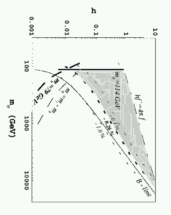
Figure 1: Constraints on technicolor with scalars in limit [i], where the scalar self-coupling is negligible, plotted on the left in the conventional basis ($\tilde{M}_{\phi}$, h) and on the right in the physical basis ($m_{\sigma}$, h). The allowed region of parameter space (shaded) is bounded by the contours $m_{\sigma}=114$ GeV (solid), $R_{b}-R_{b}^{SM}=0.26\%$ (dashes) and $hf^{\prime}=4\pi f$ (dot-dash). Other contours of constant $R_{b}$ are shown for reference. The current bound from searches for charged scalars $m_{\pi^{\pm}_{p}}=79$ GeV is shown (long dashes) along with the reference curve $m_{\pi^{\pm}_{p}}=m_{t}-m_{b}$. The constraint from $B^{0}\bar{B}^{0}$ mixing is labeled “B-line”.

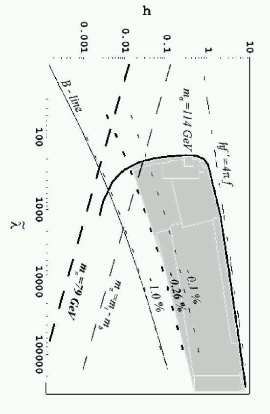
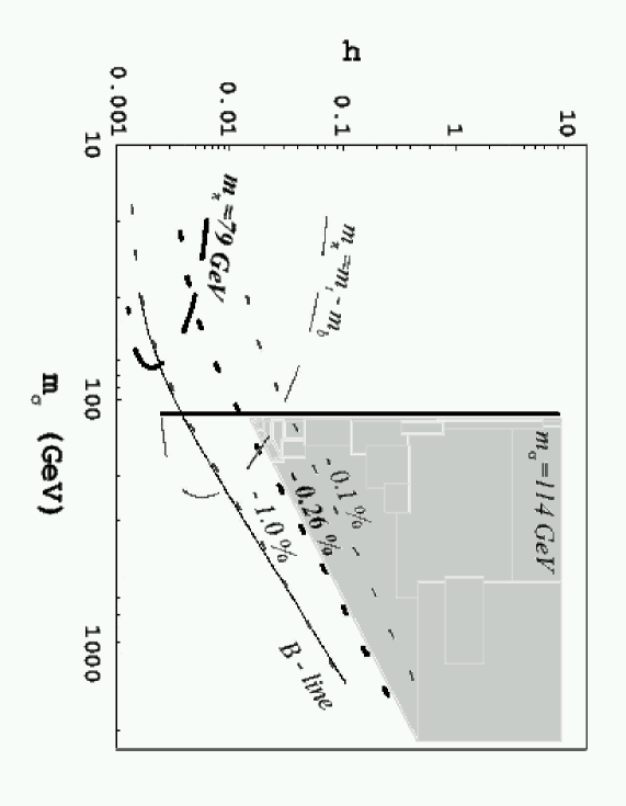
Figure 2: Constraints on technicolor with scalars in limit [ii], where the scalar mass is negligible, plotted on the left in the conventional basis ($\tilde{M}_{\phi}$, h) and on the right in the physical basis ($m_{\sigma}$, h). The allowed region of parameter space is bounded by the contours $m_{\sigma}=114$ GeV (solid) and $R_{b}-R_{b}^{SM}=0.26\%$ (dashes). Other contours of constant $R_{b}$ are shown for reference. The current bound from searches for charged scalars $m_{\pi^{\pm}_{p}}=79$ GeV is shown (long dashes) along with the reference curve $m_{\pi^{\pm}_{p}}=m_{t}-m_{b}$. The constraint from $B^{0}\bar{B}^{0}$ mixing is labeled “B-line”; the theoretical constraint $hf^{\prime}=4\pi f$ is also indicated.

3.1 $R_{b}$ and other $b$ physics

Radiative corrections to hadronic $Z$ decays resulting from the presence of the extra physical charged scalars in the low-energy spectrum tend to reduce the value of $R_{b}$ below the Standard Model prediction in models of technicolor with scalars. The amount of the reduction was calculated as a function of model parameters in [20, 13]. The current measurement of $R_{b}$ reported by the LEP Electroweak Working Group is $R_{b}^{expt}=0.21664\pm 0.00068$. This implies, at the 95% c.l., that $R_{b}$ lies no more than 0.26% below the Standard Model value of 0.21583 . Our figures show the contour $R_{b}-R_{b}^{SM}=-0.26\%$ in bold dots; the allowed regions of parameter space lie above the contour. For reference, the contours at -0.1% and -1.0% are shown in light dots.

The predicted values of several other observables related to B physics trace out curves in the model parameter space which are similar in shape to the contours of constant $R_{b}$. It is useful to compare them to get a sense of the present and future constraints from heavy flavor physics. First there is the approximate limit from $B^{0}\bar{B}^{0}$ mixing (the “B-line”), based on requiring the estimated contributions from new physics in the model not to exceed those from the Standard Model fields in the model. The constraint from $R_{b}$ supersedes that imposed by the B-line, as illustrated in the figures. Second, several authors have calculated the predicted rate of $b\to s\gamma$ in technicolor with scalars and related models [25, 26, 14, 15] as a function of the model parameters. The contour corresponding to a 50% reduction in the rate of $b\to s\gamma$ relative to the Standard Model value is approximately contiguous with the B-line. Recent measurements of $b\to s\gamma$ from ALEPH [21], BELLE[22], and CLEO[23] imply at 95% c.l. that the maximum reduction relative to the Standard Model rate[24] of 3.28 $\pm$ 0.33 $\times 10^{-4}$ is, respectively, 78%, 50% and 48%. Hence, current experimental limits from $b\to s\gamma$ are not significantly stronger than those from $B^{0}\bar{B}^{0}$ mixing, and are weaker than those from $R_{b}$. More precise measurements would have the power to test the model further. Finally, calculations of $B\to X_{s}\mu^{+}\mu^{-}$ [14], $B\to X_{s}e^{+}e^{-}$ [14], and $B\to X_{c}\tau\bar{\nu}$ [15] yield no currently useful limits. Future experiments have the potential to make the first of these a good probe of technicolor with scalars; the deviations from the Standard Model values predicted for the other two are too small to be visible.

3.2 Neutral scalars

The LEP Collaborations [19] have placed 95% c.l. lower limit of $M_{H}\leq 113.5$ GeV on the mass of a neutral Higgs boson by studying the process $Z^{*}\to ZH$ and assuming a Standard Model coupling at the $ZZH$ vertex. The $ZZ\sigma$ coupling in the technicolor with scalars model is reduced relative to the standard $ZZH$ coupling by a factor of $f^{\prime}/v$, so that the LEP limit on $m_{\sigma}$ differs, in principle, from that on $M_{H}$. In practice, however, in the region of parameter space still allowed by other constraints, $f^{\prime}/v\sim 1$ along the $m_{\sigma}=114$ GeV contour. This contour therefore serves as an approximate boundary to the experimentally allowed region [12]. In limit [i], the bound on $m_{\sigma}$ eliminates much of the parameter space for which $\tilde{M}_{\phi}\leq 70$ GeV; in contrast, a just a few years ago [13], the limit on $m_{\sigma}$ was too weak to be relevant. In limit [ii], the bound on $m_{\sigma}$ excludes regions of small $\tilde{\lambda}$ and obviates the theoretical restriction $hf^{\prime}\leq 4\pi f$. Using the right-hand plots in Figures 1 and 2, it is straightforward to project how future experimental limits on $m_{\sigma}$ will tend to constrain the model.

3.3 Charged scalars

The strongest limits on the charged physical scalars $\pi^{\pm}_{p}$ currently come from LEP searches for the charged scalars characteristic of two-higgs-doublet models. The LEP experiments have obtained limits on the charged scalar mass as a function of $\tan\beta$ and the branching ratio to $\tau\nu$ final states (assuming all decays are to $\tau\nu$ or $cs$). In theories, like technicolor with scalars, where the charged scalar coupling to fermions is of the pattern characteristic of type-I two-higgs models, the branching fraction to $\tau\nu$ is predicted to be 1/3. Hence, one can read from figure 7 of ref. [27] that the limit on $m_{\pi^{\pm}_{p}}$ is 78 GeV; preliminary new data from LEP II [28] pushes the lower bound to 79 GeV.

The $m_{\pi^{\pm}_{p}}=79$ GeV contour is shown in all of our figures for reference, although the bounds on technicolor with scalars from data on $m_{\sigma}$ and $R_{b}$ are currently stronger. The contour $m_{\pi^{\pm}_{p}}=m_{t}-m_{b}$ is also shown in each plot in order to indicate how stronger bounds on charged scalar masses would tend to constrain the model. Based on the intersection of the current $m_{\sigma}$ and $R_{b}$ bounds, an experiment sensitive to $m_{\pi^{\pm}_{p}}=128$ (138) GeV would probe regions of limit [i] (limit [ii]) parameter space beyond what is currently excluded. If the lower bound on $m_{\sigma}$ were to tighten to 133 (160) GeV in the future, then only a search for charged scalars with $m_{\pi^{\pm}_{p}}\geq m_{t}-m_{b}$ would probe regions of limit [i] (limit [ii]) beyond what limits from neutral scalars and $R_{b}$ excluded.

The Tevatron experiments can search for light type-II charged scalars in top quark decays. While the Run I searches for charged scalars lacked the reach of the LEP searches, that will change as Run II accumulates data. For values of $\tan\beta=f/f^{\prime}\stackrel{{\scriptstyle<}}{{\sim}}2$, the rate of $t\to H^{\pm}b$ is nearly identical for type-I and type-II scalars; at higher $\tan\beta$, the rate for type-I scalars drops off rapidly and the Tevatron limits do not directly apply to technicolor with scalars. DØ has set limits at low $\tan\beta$ based on the decay path $H^{\pm}\to cs$. The value of $B(H^{+}\to cs)$ in type-I models (2/3) matches the value in type-II models at $\tan\beta)=1$. Hence, one can read from figure 3 of [29] that the current limit from DØ data is $m_{\pi^{\pm}_{p}}>60$ GeV for $\tan\beta\leq 2$. It is projected that with $2fb^{-1}$ of integrated luminosity the Run II experiments will be sensitive to $\pi^{\pm}_{p}$ weighing up to 135 GeV [30], a significant improvement over the LEP bounds at low $\tan\beta$.

4 Conclusions

Technicolor with scalars remains a viable effective theory of dynamical electroweak symmetry breaking and fermion mass generation. Recent searches for charged and neutral scalars and measurements of heavy flavor observables such as $R_{b}$ have certainly reduced the extent of the allowed parameter space. However, the model is consistent with data for a wide range of isosinglet scalar masses $m_{\sigma}$ and technifermion coupling to scalars $h$.

In limit [i] of the model, where the scalar self-coupling $\lambda$ is small, $m_{\sigma}$ is bounded from below by LEP searches for the higgs and from above by a combination of the measured value of $R_{b}$ and the theoretical consistency requirement $hf^{\prime}=4\pi f$. As shown in figure 1, 114 GeV $\stackrel{{\scriptstyle<}}{{\sim}}m_{\sigma}\stackrel{{\scriptstyle<}}{{\sim}}$ 14 TeV. In limit [ii], the constraint $hf^{\prime}=4\pi f$ is superseded by the LEP limit $m_{\sigma}\stackrel{{\scriptstyle>}}{{\sim}}$ 114 GeV. Hence, larger values of $h$ are allowed for a given $m_{\sigma}$ than in limit [i], as indicated in figure 2, and the maximum allowed value of $m_{\sigma}$ is also somewhat larger.

Upcoming searches for charged and neutral scalar bosons will begin exploring the lower allowed values in the $m_{\sigma}$ mass range. At present, searches for neutral scalars with masses above 114 GeV or charged scalars with masses above 128 GeV (138 GeV) would give new information about limit [i] (limit [ii]) of technicolor with scalars. Complimenting this, new measurements of $b\to s\gamma$ and $b\to s\mu^{+}\mu^{-}$ will be sensitive even to the heaviest allowed scalar masses. If either branching ratio were measured to be within a few percent of the standard model value, the resulting exclusion curve in the $m_{\sigma},h$ plane would run close to the $\delta R_{b}/R_{b}=-0.1\%$ curves in figures 1 and 2 [13, 14, 15], tending to reduce the largest allowed value of $m_{\sigma}$.

Acknowledgments

EHS acknowledges the financial support of an NSF POWRE Award. VH acknowledges the financial support of a Radcliffe Research Partners Award. This work was supported in part by the National Science Foundation under grant PHY-0074274, and by the Department of Energy under grant DE-FG02-91ER40676.

References

- [1] S. Weinberg, Phys. Rev. D 19 (1979) 1277; L. Susskind, Phys. Rev. D 20 (1979) 2619.
- [2] S. Dimopoulos and L. Susskind, Nucl. Phys. B 155 (1979) 237; E. Eichten and K. Lane, Phys. Lett. B 90 (1980) 125.
- [3] T. Appelquist, M. J. Bowick, E. Cohler and A. I. Hauser, Phys. Rev. Lett. 53 (1984) 1523.
- [4] B. Holdom and J. Terning, Nucl. Phys. B 347 (1990) 88; M. Golden and L. Randall, Nucl. Phys. B 361 (1991) 3; M.E. Peskin and T. Takeuchi, Phys. Rev. Lett. 65 (1990) 964; W.J. Marciano and J.L. Rosner, Phys. Rev. Lett. 65 (1990) 2963; D. Kennedy and P. Langacker, Phys. Rev. Lett. 65 (1990) 2967.
- [5] R. S. Chivukula, S. B. Selipsky and E. H. Simmons, Phys. Rev. Lett. 69 (1992) 575 [hep-ph/9204214].
- [6] E. H. Simmons, Nucl. Phys. B 312 (1989) 253.
- [7] R.S. Chivukula, A.G. Cohen and K. Lane, Nucl. Phys. B343 554 (1990); T. Appelquist, J. Terning, and L.C.R. Wijewardhana, Phys. Rev. D44 871 (1991).
- [8] S. Samuel, Nucl. Phys. B 347 (1990) 625; M. Dine, A. Kagan, and S. Samuel, Phys. Lett. B 243 (1990) 250; A. Kagan and S. Samuel, Phys. Lett. B 252 (1990) 605; A. Kagan and S. Samuel, Phys. Lett. B 270 (1991) 37; A. Kagan and S. Samuel, Int. J. Mod. Phys. A 7 (1992) 1123.
- [9] B. A. Dobrescu, Nucl. Phys. B 449 (1995) 462 [hep-ph/9504399].
- [10] J. D. Lykken, Phys. Rev. D 54 (1996) 3693 [hep-th/9603133]; N. Arkani-Hamed, S. Dimoppoulos, and G. Dvali, Phys. Lett. B 429 (1998) 263 [hep-ph/9803315].
- [11] N. Evans, Phys. Lett. B 331 (1994) 378 [hep-ph/9403318].
- [12] C.D. Carone and H. Georgi, Phys. Rev. D49 1427 (1994); C. D. Carone and E. H. Simmons, Nucl. Phys. B 397 (1993) 591 [hep-ph/9207273]; C.D. Carone and M. Golden, Phys. Rev. D49 6211 (1994).
- [13] C. D. Carone, E. H. Simmons and Y. Su, Phys. Lett. B 344 (1995) 287 [hep-ph/9410242].
- [14] Y. Su, Phys. Rev. D 56 (1997) 335 [hep-ph/9612485].
- [15] Z. Xiong, H. Chen and L. Lu, Nucl. Phys. B 561 (1999) 3.
- [16] B. A. Dobrescu and E. H. Simmons, Phys. Rev. D 59 (1999) 015014 [hep-ph/9807469].
- [17] A. Manohar and H. Georgi, Nucl. Phys. B234 189 (1984); H. Georgi and L. Randall, Nucl. Phys. B276 241 (1986); H. Georgi, Phys. Lett. B298 187 (1993).
- [18] S. Coleman and E. Weinberg, Phys. Rev. D7 (1973) 1888.
- [19] T. Kawamoto, Proceedings, XXXVIth Rencontres de Moriond, QCD and Hadronic Interactions at High Energy, March 17th-24th 2001 (2001); 2001, Tatsuo Kawamoto ; E. Tournefier, Proceedings, XXXVI Rencontres de Moriond Electroweak Interactions and Unified Theories Les Arcs, March 11-17-2001 (2001); see also the LEP Electroweak Working Group home page http://lepewwg.web.cern.ch/LEPEWWG/ .
- [20] M. Boulware and D. Finnell, Phys. Rev. D44 2054 (1991); W. Hollik, Mod. Phys. Lett. A5 1909 (1990).
- [21] ALEPH Collaboration, Phys. Lett. B429 (1998) 429.
- [22] M. Nakao, Proceedings, ICHEP 2000, Osaka, Japan (2000). #281 / BELLE-CONF-0003 .
- [23] T. Coan, Proceedings, ICHEP 2000, Osaka, Japan (2000).
- [24] K. Chetyrkin et al., Phys. Lett. B400 (1997) 206 and B427 (1998) 414; A. Kagan and M. Neubert, Eur. Phys. J C7 (1999) 5.
- [25] B. Grinstein, R. Springer, and M.B. Wise, Nucl. Phys. B339 269 (1990).
- [26] T.G. Rizzo, Phys. Rev. D38 820 (1988);W.S. Hou and R.S. Willey, Phys. Lett. B202 591 (1988); C.Q. Geng and J.N. Ng, Phys. Rev. D38 2858 (1988); V. Barger, J.L. Hewett, and R.J.N. Phillips, Phys. Rev. D41 3421 (1990).
- [27] D.E. Groom et al., European Phys. Journal C 15 (2000) 1 and 1999 off-year partial update for the 2000 edition (URL:http://pdg.lbl.gov/).
- [28] P. Bock et al. [ALEPH, DELPHI, L3 and OPAL Collaborations], CERN-EP-2000-055.
- [29] B. Abbott et al. [D0 Collaboration], Phys. Rev. Lett. 82 (1999) 4975 [hep-ex/9902028].
- [30] S. S. Snyder [D0 Collaboration], hep-ex/9910029.