High Density QCD

Abstract

The dynamics of high partonic density QCD is presented considering, in the double logarithm approximation, the parton recombination mechanism built in the AGL formalism, developed including unitarity corrections for the nucleon as well for nucleus. It is shown that these corrections are under theoretical control. The resulting non linear evolution equation is solved in the asymptotic regime, and a comprehensive phenomenology concerning Deep Inelastic Scattering like $F_{2}$, $F_{L}$, $F_{2}^{c}$. $\partial F_{2}/\partial\ln Q^{2}$, $\partial F^{A}_{2}/\partial\ln Q^{2}$, etc, is presented.

The connection of our formalism with the DGLAP and BFKL dynamics, and with other perturbative (K) and non-perturbative (MV-JKLW) approaches is analised in detail. The phenomena of saturation due to shadowing corrections and the relevance of this effect in ion physics and heavy quark production is emphasized. The implications to $e$-RHIC, HERA-A, and LHC physics and some open questions are mentioned.

Plenary Talk presented at XXI ENFPC, São Lourenço, Brasil, October, 24^th (2000).

I Introduction

The dynamics of the high density Quantum Chromodynamics (hdQCD) is one of the present most challeging open questions in high energy physics. The intense theoretical and experimental activity towards the understanding of small $x$ (small fraction of proton momentum carried by the struck parton) QCD takes place from Deep Inelastic Scattering (DIS) at HERA [1] to heavy ions collisions (HIC) at RHIC [2]. This kinematical regime will also be tested at LHC in a near future [3].

Important contribution to the interest of the field is due to the puzzling result obtained by HERA at small-$x$ ($x\leq 10^{-2}$) [4] for the proton structure function $F_{2}(x,Q^{2})$. This function was observed to increase dramatically as $x$ gets smaller (Fig. 1). In the region of moderate Bjorken $x$ ($x\geq 10^{-2}$) the Operator Product Expansion (OPE) methods as well as the Renormalization Group Equations (RGE) have been applied successfully [5]. The evolution of quark and gluon distribution functions given by the DGLAP equations [6] is based on the summing of the leading powers of $\alpha_{s}\ln Q^{2}\approx 1$, $\alpha_{s}\ln(1/x)<<1$, $\alpha_{s}<<1$, where $\alpha_{s}$ is the strong coupling constant. The leading $\ln(1/x)$ contributions is the case for the BFKL equation [7]. The procedure known as the double leading logarithmic approximation (DLA) corresponds in axial gauges to generate the logarithms by ladder diagrams, whose emitted gluons have strongly ordered transverse and longitudinal momenta, summing the logs $\alpha_{s}\ln Q^{2}\ln(1/x)$. It was shown that the DLA is a common limit between the linear dynamics [8].

The increasing of the parton densities requires a formulation of the QCD at high partonic density, where unitarity corrections (UC), not considered in the previous dynamics already mentioned, are properly taken into account. In this sense, the small $x$ region, where the gluon distribution sets the behavior of the main observables, provides the interface between perturbative and non perturbative QCD, or in other words, between hard and soft physics. Clearly, both experimentalists and theoreticians are challenged to desentangle, measure and formulate the dynamical collective effects that are subjacent to the observed result of increasing $F_{2}$ and the cross section $\sigma_{tot}$ at DIS, as $x$ gets smaller [4]. Both evolution equations, DGLAP (evolution in $\ln Q^{2}$) and BFKL (evolution in $\ln(1/x)$) as representatives of linear dynamics, need control in order to restore unitarity, since the Froissart limit requires $\sigma_{tot}\leq Cte\,\ln^{2}s$ [9].

A comprehensive treatment should envolve both linear and non linear regimes. The main attempts to develop a formalism for hdQCD are the approaches of Mc.Lerran and collaborators ($MVJKLW$) [10], by Kovchegov ($K$) [11] and by Ayala, Gay Ducati and Levin ($AGL$) [12, 13]. Derived independently, the three methods obtain non linear evolution equations for the gluon distribution, at the small $x$ region, describing the onset of hdQCD, although considering different degrees of freedom.

In what follows I will present an introductory review of the subject of hdQCD, the main aspects of the formulations to the subject, the connections among them in the asymptotic region ($x\rightarrow 0$), present the state of art of the phenomenology of small $x$ physics and address some open questions.

II The Evolution Equations

It will be briefly presented the DGLAP and BFKL dynamics and their predictions for the small $x$ regime at DIS. The DIS is the process of interaction of a lepton and a nucleon exchanging an electroweak boson producing many particles at the final state, which is a hadronic state $X$. The process is

$$l(k)\,\,N(p)\rightarrow l^{\prime}(k^{\prime})\,\,X\,\,,$$ (1)

where $k$, $k^{\prime}$, $p$ and $p^{\prime}$ are the fourmomenta of the initial and final lepton, incident nucleon and final hadronic system, respectively. The main variables for this process are $Q^{2}=-q^{2}=-(k-k^{\prime})^{2}$, which is the square of the transfered momentum, $s=(k+p)^{2}$, the square of the center of mass energy, $W^{2}=(q+p)^{2}=(p^{\prime})^{2}$, the square of the center of mass energy of the virtual boson-nucleon system. The hard scale is given by $q^{2}$ ($<0$), corresponding to the process resolution, and $x=Q^{2}/2p.q$, meaning the virtual boson resolves the hadronic structure, or the partons, since $\Delta x\approx 1/\sqrt{Q^{2}}$ . Are also useful the variables $y=q.p/k.p$, measuring the process inelasticity and $\nu=q.p/m_{N}$, the energy of the virtual boson once taken in the target rest frame.

In terms of the partonic content of the nucleon the structure function, which reflets its overall distribution, is given by

$$F_{2}(x,Q^{2})=\sum_{f}\,e_{f}^{2}\,[\,q^{f}(x,Q^{2})\,]\,,$$ (2)

where the sum is over flavours weighted by the respective squared charges ($e^{2}_{f}$). It is this function that is object of main experimental studies, specially at HERA, at the small longitudinal nucleon fraction of momentum, or small $x$ (see Fig. 1) [14].

FIG. 1.:

The quark distribution function can be shown to evolve as

$$\frac{\partial q^{f}(x,Q^{2})}{\partial\ln Q^{2}}=\frac{\alpha_{s}}{2\pi}\int\frac{dx_{1}}{x_{1}}\,P_{qq}(\frac{x}{x_{1}})\,q^{f}(x,Q^{2})\,\,,$$ (3)

where $P_{qq}=C_{F}\frac{1+z^{2}}{1-z}\left|{}_{+}\right.$ (with self-energy corrections over the $k$ propagator) is one of the splitting functions $P_{ij}$ ( $P_{gq}=C_{F}\frac{1+(1-z)^{2}}{z}$, etc), describing the transition between the quark state $i$ to the quark state $j$, from fraction of momentum $x_{1}$ to $x$. The above evolution refers to the non singlet quarks distribution where sea quarks and gluon distribution are uncoupled

$$q_{NS}(x,Q^{2})\equiv q_{i}(x,Q^{2})-q_{j}(x,q^{2})\,\,.$$ (4)

The singlet quark distribution is given by

$$q_{S}(x,q^{2})\equiv\sum_{f}\left[\,q^{f}(x,Q^{2})+\bar{q}^{f}(x,Q^{2})\,\right]\,\,,$$ (5)

where the gluon distribution is coupled to the quark one. Now the evolution equations, in the linear regime, read for the quarks

$$\frac{\partial q_{S}(x,Q^{2})}{\partial\ln Q^{2}}=\frac{\alpha_{s}(Q^{2})}{2\pi}\left[\int_{x}^{1}\left(P_{qq}(\frac{x}{x_{1}})q_{s}(x_{1},Q^{2})\right.\right.$$ (6)

$$+\left.\left.P_{qg}(\frac{x}{x_{1}})g(x,Q^{2})\right)\right]\,\,,$$ (7)

and for the gluon distribution

$$\frac{\partial g(x,Q^{2})}{\partial\ln Q^{2}}=\frac{\alpha_{s}(Q^{2})}{2\pi}\,\left[\int_{x}^{1}\left(P_{gq}(\frac{x}{x_{1}})q_{s}(x_{1},Q^{2})\right.\right.$$ (8)

$$+\left.\left.P_{gg}(\frac{x}{x_{1}})g(x,Q^{2})\right)\right]\,\,.$$ (9)

The Eqs. (7) and (9) were independently derived by Dokshitzer, Gribov and Lipatov, and by Altarelli and Parisi, known as DGLAP equations in leading order. The perturbative QCD evolution, in the linear sector is governed by DGLAP equations, moreover a suitable non perturbative inicial condition, extracted from the experiment for a given boson virtuality.

It can be shown by sucessive derivations that $q_{NS}(x,\varepsilon)\sim\sum_{n}(\alpha_{s}\varepsilon)^{n}$, $\varepsilon=\ln Q^{2}$, which corresponds to the emission of $n$ gluons, showing that the DGLAP equations resum the leading $\ln Q^{2}$. This can be understood as ladder diagrams with a strong ordering in transverse momenta $k_{\perp}$, i.e., $Q_{0}^{2}<<k_{1}^{2}<<...<<k_{n}^{2}<<Q^{2}$. The scale $Q_{0}^{2}$ is the cut, or transition value between perturbative and non perturbative physics. It was shown by Gribov [15] that this result is gauge independent once one considers the leading logarithm approximation.

At small-$x$ the gluons dominate, since $P^{(0)}_{gg}(z)\sim\frac{2N_{c}}{z}$, and the parton distributions have the general behavior $xp_{i}(x,Q^{2})\sim x^{-\lambda}$, $\lambda>0$. More likely for initial condition $xp_{i}(x,Q_{0}^{2})\sim Const$ and $xp_{i}(x,Q^{2})\sim exp\sqrt{\ln(\ln Q^{2})\ln 1/x}$, known as double leading logarithm approximation (DLA). From that is clear that DGLAP predicts the increase of the gluon distribution function, and of the structure function $F_{2}$ with the decreasing of $x$, whose relation in this kinematical regime is given by

$$\frac{\partial F_{2}(x,Q^{2})}{\partial\ln Q^{2}}=\frac{\alpha_{s}(Q^{2})}{2\pi}\sum_{f}e_{f}^{2}xg(x,Q^{2})$$ (10)

being equal to $\frac{2\alpha_{s}}{9\pi}xg(x,Q^{2})$ for $n_{f}=3$. The DLA implies strong ordering in $x$ and $k_{T}$, i. e., $x_{1}>>x_{2}>>....>>x_{i-1}>>x_{i}>>x$ and $k_{T_{1}}<<k_{T_{2}}<<...k_{T_{i-1}}<<k_{T_{i}}<<Q^{2}$, the resum of logs of $\alpha_{s}\ln(1/x)\ln Q^{2}$, having as region of validity $\alpha_{s}<<1$, $\alpha_{s}\ln(1/x)<<1$ and $\alpha_{s}\ln(1/x)\ln Q^{2}\approx 1$.

The resum of all leading logarithms of Bjorken $x$, or the energy, is characteristic of the Balitsky-Fadin-Kuraev-Lipatov (BFKL) equation. For very low $x$ values the $\ln s$ becomes large and $\alpha_{s}\ln 1/x\approx 1$ and the DLA is not valid. The BFKL evolution equation is proposed for an unintegrated gluon distribution function in the transverse momentum variable. Its solution grows as a power of the center of mass energy $s$ with the consequent violation of the unitarity bound [9] at very high energies. The cure for this problem was not reached in the next to leading order calculation [16], and is still under research for instance, through the resumming of all BFKL Pomeron exchanges [17], for the cross section as well as for the structure function.

The amplitude for the scattering quark-quark with one gluon exchange in the $t$ channel at lowest order is given by ${\cal A}_{0}(s,t)\sim s/t$, and for the next order in $\alpha_{s}$ the leading terms are given by $\ln s$, resulting ${\cal A}_{1}(s,t)\sim{\cal A}_{0}(s,t)\ln s$. Once one goes to higher orders the number of contributing diagrams increases and the calculation gains enormously in complexity [18], and the usual procedure is to introduce an effective vertex (Lipatov vertex). It results that the general term is ${\cal A}_{n}(s,t)\sim{\cal A}_{0}(s,t)\epsilon^{n}(t)\ln^{n}(s)/n$, where $\epsilon(t)$ is a suitable function to take care of infrared divergencies, docile under regularization, for instance, dimensional regularization.

Clearly the BFKL evolution is summing the terms $\alpha_{s}^{n}\ln^{n}(s)$, where lower order logarithms are neglected. The result for the amplitude is

$${\cal A}(s,t)={\cal A}_{0}(s,t)\sum_{n=0}^{\infty}\frac{\epsilon^{n}(t)\ln^{n}(s)}{n}\approx s^{\alpha(t)}\,\,,$$ (11)

with $\alpha(t)=1+\epsilon(t)$. In this case, there is still the $\epsilon(t)$ infrared divergencies to be cured.

When just the singlet contribution in the $t$-channel is considered in the BFKL formalism, meaning that only Pomeron exchange diagrams are taken into account, the amplitude is given by

$$\frac{Im{\cal A}(s,t)}{s} = \frac{{\cal G}}{2\pi^{2}}\int d^{2}k_{1}d^{2}k_{2}\,\Phi_{A}(k_{1},q)$$ (12)

$$\times \frac{F(y,k_{1},k_{2},q)}{k_{2}^{2}(k-q)^{2}}\,\Phi_{B}(k_{2},q)\,\,,$$ (13)

where ${\cal G}$ is the color factor for the process and $q$ is the transfered momentum in the $t$-channel; the functions $\Phi_{i}$ are the impact factors setting the coupling of $F$ to the external particles and finally the function $F$ is the perturbative gluon ladder. At leading order it consists into the exchange of two gluons but the sum of all terms implies an integral equation for $F$, that is infrared finite for a reggeized gluon ladder. This behavior of the kernel of the BFKL equation is connected with the QCD Pomeron and it is the resum of the leading logarithms $\ln s$.

The solution of the BFKL equation predicts the steep growth of the gluon distribution with decreasing $x$ as well as the diffusion of the transverse momenta. As well as DGLAP equations, the BFKL equation predicts the growing of the cross section in the small-$x$ regime since the dynamics of this observable is related with the gluon distribution function.

From this very brief discussion on the main issues of the linear formalisms for the dynamics of the parton distributions, it gets clear the need of formal improving in order to include the unitarity corrections preserving the Froissart limit. This important aspect of high energy physics was pointed out many years ago by Gribov, Levin and Ryskin (GLR) in Ref. [19]. I will present in the following the main attempts developed in the recent years towards a non linear dynamics for high density QCD, as well as the high energy phenomenology provided.

III The Question

The main question that is addressed once treating hdQCD is how to analytically separate small and large distance contributions to high energy amplitudes in a properly gauge invariant formalism. This corresponds to establish the hard and soft scales for the process of interest and develop the physical meaningful method to introduce the unitary corrections (UC) into the parton dynamics. Once the theoretical need for UC is established we should look for their signatures analysing different observables. Besides comparing the predictions of the distinct formalisms it is required a common limit between them, probably to be set by a saturation scale, $Q^{2}_{S}$. There exists mainly two non linear perturbative approaches [11, 12, 13] and a non perturbative one [10]. Although some progress has been made towards their connection there is no common analytic solution for the gluon distribution $g(x,Q^{2})$ for all kinematical range.

The physics of hdQCD shakes the parton model and the cherished concept of incoherence that is behind the standard calculations. It seems that in order to control the increasing of the gluon function some gluon recombination mechanism has to take place as the energy gets higher and higher.

This is a good point to remind that the analysis of the structure functions has already given us some surprises, and the previous important one was the EMC effect [20], that has as a main result $F_{2}^{A}/AF_{2}^{n}\neq 1$. This difference is not predicted if one requires complete incoherence of the partons, and reveals the presence of nuclear effects in the structure functions where they were not expected. A large literature is devoted to this phenomena, but it is interesting to point out that the shadowing behavior noticed in $J/\Psi$ production could be nicely described [21], as well as the comparison with Drell-Yan processes [22], for the first data at small-$x$, considering the recombination approach developed by Mueller and Qiu [23] which is based on the GLR proposals.

Two main aspects are in order, the control of the increasing of the gluon distribution function as an unitarity imperative and the appearance of nuclear effects in high energy processes. If this aspect is relevant for fixed target quarkonia production, it is strongly important for physics of HERA-A, RHIC and LHC with nuclei.

IV The High Density QCD Approaches

The leading logarithm approximation DLA (related to DGLAP) and LL(1/x) (related to BFKL) result both into linear evolution equations for the gluon distribution function. The effect of summing large logs in high energy regime implies the increase of the gluon distribution function $g(x,Q^{2})$ as well as the cross section once $x$ decreases. However, this result violates the unitarity of the scattering matrix, a main theorem of relativistic Quantum Field Theory, the Froissart theorem [9], which states the cross section cannot grow faster than $\ln^{2}s$. Translated to the DIS, this implies increasing restrictions to the structure function and/or total cross section, say lower than $\ln^{2}(1/x)$ and provides a limitation in the $x$ range to the application of linear evolutions in order to get suitable results.

Intuitively we can associate $xg(x,Q^{2})$ to the number of gluons into the nucleon, $n_{g}$, per rapidity unity, $y=\ln(1/x)$, with transverse size of order $1/Q$. In the hadron-nucleon interaction it is the virtual gluon that probes the nucleon structure, in analogy with the eletroweak boson in DIS. The virtual gluon-nucleon cross section is

$$\sigma_{G^{*}N}(x,Q^{2})=\sigma_{0}\,xg(x,Q^{2})\,\,,$$ (14)

where $\sigma_{0}=\sigma_{G^{*}g\rightarrow X}=Cte\,\frac{\alpha_{s}(Q^{2})}{Q^{2}}$, is the total cross section of the virtual gluon, with virtuality $Q^{2}$, and nucleon gluon interaction. Assuming $\sigma_{0}=\pi R^{2}_{HAD}$, then $\sigma_{0}xg(x,Q^{2})$ corresponds to the area occupied by the gluons in a nucleon. As $x\rightarrow 0$, this transverse area may be comparable, or even bigger, than $\pi R^{2}_{HAD}$, following DGLAP or BFKL predictions for small $x$ or small $Q^{2}$. Approaching this regime the gluons may begin to superpose spatially in the transverse direction and to interact, behaving not anymore as free partons. These interactions should slower, or even stop, the intense growing of the cross section, fixing the limit $\pi R^{2}_{HAD}$ in the small $x$ regime.

Introducing the function $\kappa$, with probabilistic interpretation

$$\kappa=\sigma_{0}\frac{xg(x,Q^{2})}{\pi R^{2}}\,\,,$$ (15)

it is possible to estimate in which kinematical region one can expect modifications in the usual evolution equations. So to say, for $\kappa<<1$ the system stays at $x$ and $Q^{2}$ where the usual evolution equations (linear) are applicable, governed by individual partonic cascades, without interactions among the cascades.

As $\kappa\approx\alpha_{s}$, partons from distinct cascades begin to interact due to spatial superposition. This specific kinematical regime or the onset of the recombination mechanism was first studied by Gribov, Levin and Ryskin [19] almost twenty years ago, proposing the introduction of non linear terms into the evolution equation.

The region of $\kappa\rightarrow 1$ was addressed more recently [12, 13] (see Fig. 2) and experienced considerable development on the theoretical side [10, 11], also motivated by HERA results and the great interest on RHIC and LHC future data. This is the kinematical regime that requires the QCD dynamics for high partons density. Although the coupling constant $\alpha_{s}$ is still small, allowing in principle the use of perturbative methods, the system is so dense that manifestation of non-linear effects are expected, and they are required to be considered in a complete formalism.

The region of $\kappa\rightarrow 1$ corresponds to partons in a non-equilibrium state and new methods are in order to treat the collective phenomena.

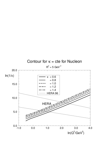
FIG. 2.:

A The GLR Formulation

Gribov, Levin and Ryskin [19] introduced the mechanism of parton recombination in perturbative QCD for high density systems, expressing this as unitarity corrections included in a new evolution equation known as GLR equation. In terms of diagrams it considers the dominant non-ladder contributions, or multi-ladder graphs, also denoted fan diagrams.

The standard QCD evolution is represented by a cascade of partonic decays in the nucleon. The photon interacts with a parton with fraction of momentum $x$ and virtuality $Q^{2}$, which is the last one of a chain where the partons get slower and with bigger virtuality. The scale $Q_{0}$ sets the initial virtuality and at the same time, the limit for perturbative QCD applicability, and $Q^{2}$ is the higher virtuality of the chain. In the transverse plane the partons with low fraction of momentum stay in the lower part of the ladder and have large transverse size; those with bigger virtuality are on the upper part of the ladder and transversally smaller.

Following DGLAP, the number of partons of low fraction of momentum increases very rapidly, which pictorically corresponds to bigger density of individuals in the same allowed area, in contrast with a more diluted system at intermediate values of $x$, far away from the possibility of superposition. The transition between these regimes should be characterized by a critical value $x=x_{CRIT}$. The same can be argued through BFKL formalism, with the difference that in this case the increasing of the partonic distributions, takes place at a fixed transverse scale, although the evolution presents the fluctuations in the transverse plane due to the characteristic diffusion in BFKL.

It is important to emphasize that in both linear dynamics only the decay processes are considered in the partonic evolution, however we expect that the anihilation mechanism should contribute in the low $x$ regime, providing some control of the increasing of the partons distribution function. In the linear approach we consider one incident and two emergent partons to construct the splitting functions for the decay processes. Now it is the case to consider two incident partons and one emergent one, and to express the recombination mechanism it is needed a formulation in terms of the probability to recombine two incident partons.

As a first approximation one considers the anihilation probability as proportional to the square of the probability to find one incident parton, introducing a non-linear behavior.

Taking $\rho=\frac{xg(x,Q^{2})}{\pi R^{2}}$ as the gluon density in the transverse plane, one has the general behavior: for splitting $1\rightarrow 2$, the probability is proportional to $\alpha_{s}\,\rho$, for anihilation $2\rightarrow 1$, the probability is proportional to $\alpha_{s}^{2}\rho^{2}/Q^{2}$; where $1/Q^{2}$ stands for the size of the produced parton. For $x\rightarrow 0$, $\rho$ increases and the anihilation process becomes relevant. Considering a cell of volume $\Delta\ln Q^{2}\Delta\ln(1/x)$ in the phase space allows one to write the modification of the partonic density as

$$\frac{\partial^{2}\rho}{\partial\ln Q^{2}\partial\ln 1/x}=\frac{\alpha_{s}N_{c}}{\pi}\rho-\frac{\alpha_{s}^{2}\gamma\pi}{Q^{2}}\rho^{2}\,\,,$$ (16)

where the coupling in the process is given by $\gamma$. Expressing in terms of the gluon distribution the above equation is

$$\frac{\partial^{2}xg(x,Q^{2})}{\partial\ln Q^{2}\partial\ln 1/x}=\frac{\alpha_{s}N_{c}}{\pi}xg-\frac{\alpha_{s}^{2}\gamma}{Q^{2}R^{2}}[xg]^{2}\,\,.$$ (17)

This equation is the GLR equation [19]. The already mentioned work of Mueller and Qiu [23] gives $\gamma=81/16$ for $N_{c}=3$.

The non-linear corrections correspond to a class of QCD Feynman diagrams, called fan diagrams, formed by a gluon ladder with subsequent subdivisions in gluon ladders, where the three ladders vertex is associated with the decay and consists of a sum of several non planar diagrams. The overall result carries a minus sign, which is important in order to control the growing of the parton distribution once the fan diagrams become relevant, i.e., at low $x$. The lowest part of the diagrams couples to the nucleon and the Eq. (14) resums all class of the diagrams represented in Fig. 3.

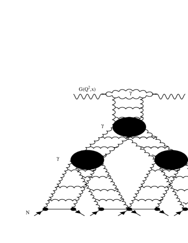
FIG. 3.:

As is clear from Eq. (14), the non-linear term reduces the growing of $xg(x,Q^{2})$ at low $x$, in comparison with the linear equations. It is also predicted for the asymptotic region $x\rightarrow 0$ the saturation of the gluon distribution, with a critical line between the perturbative region and saturation region, setting its region of validity (meaning independence of the gluon function with the energy). The subject of saturation is very appealing and there are several attempts in the literature today with distinct phenomenological approaches addressing this question [24].

In the asymptotic limit one obtains $xg(x,Q^{2})\left|{}^{GLR}_{SAT}\right.=\frac{16}{27\pi\alpha_{s}}Q^{2}R^{2}$. Since the GLR only includes the first non-linear term, although it predicts saturation in the asymptotic regime its region of validity does not extend to very high density where higher order terms should contribute significantly.

B The AGL Formulation

This approach developed by Ayala, Gay Ducati and Levin (AGL) [12, 13], intents to extend the perturbative treatment of QCD up to the onset of high density partons regime, through the calculation of the gluon distribution which is the solution of a non-linear equation that resums the multiple exchange of gluon ladders, in double leading logarithm approximation (DLA).

It is based on the development of the Glauber formalism for perturbative QCD [25], considering the interaction of the fastest partons of the ladders with the target, nucleon or nucleus, since one of the main goals is to obtain the nuclear gluon distribution $xg^{A}(x,Q^{2})$. We considered a virtual probe $G^{*}$ that interacts with the target in the rest frame, through multiple rescatterings with the nucleons. In this reference frame the virtual probe can be interpreted following the decomposition of the Fock states, and its interaction with the target occours by the decay of the component $gg$, as represented in Fig. (4).

For small-$x$ this pair has a lifetime much bigger than the nucleus (nucleon) radius and the pair is separated by the fixed transverse separation $r_{t}$ during the interaction, which is represented by the exchange of a ladder of gluons strongly ordered in transverse momentum.

The cross section for this process is given by

$$\sigma^{G^{*}A}=\int_{0}^{1}dz\,\int\frac{d^{2}r_{t}}{\pi}\,|\Psi_{t}^{G^{*}}(Q^{2},r_{t},x,z)|^{2}\,\sigma^{gg\,+\,A}\,\,,$$ (18)

where $G^{*}$ is a colorless virtual probe with virtuality $Q^{2},\,z$ is the probe fraction of energy carried by the gluon and $\Psi_{t}^{G^{*}}$ is the wave function of the transversely polarized gluon in the probe, $\sigma^{gg\,+\,A}(z,r_{t}^{2})$ is the cross section of the pair with the target, which was proven for perturbative QCD by Mueller in Ref. [25, 26]

The lower limit estimation of UC is obtained through the incoherent rescatterings of the gluon pair, with the constraint that only the fastest partons of the ladders interact with the target. Introducing the transverse impact parameter $b_{t}$ and a profile function for the nucleus $S(b_{t})$ we get

$$\sigma^{G^{*}A}=\int_{0}^{1}dz\,\int_{0}^{1}\frac{d^{2}r_{t}}{\pi}\,\int\frac{d^{2}b_{t}}{\pi}|\Psi_{t}^{G^{*}}(Q^{2},r_{t},z)|^{2}$$ (19)

$$\,2[1-e^{\frac{1}{2}\sigma_{N}^{gg}(x^{\prime},4/r_{t}^{2})S(b_{t})}]\,\,,$$ (20)

where $x^{\prime}=x/(zr_{t}Q^{2})$, $S(b_{t})$ may be taken as $\frac{A}{\pi R_{A}^{2}}e^{-b_{t}/R_{A}^{2}}$ for a gaussian profile, $\sigma_{N}^{gg}=\frac{C_{A}}{C_{F}}\sigma_{N}^{q\bar{q}}$, where $\sigma_{N}^{q\bar{q}}=\frac{C_{F}}{C_{A}}(\frac{3}{4}\alpha_{s}(4/r_{t}^{2}))\pi^{2}r_{t}^{2}xg(x,4/r_{t}^{2})$, and $4/r_{t}^{2}$ is a cut for the nonperturbative region. For the virtual probe with virtuality $Q^{2}$ the relation $\sigma^{G^{*}A}(x,Q^{2})=(\frac{4\pi^{2}\alpha_{s}}{Q^{2}})xg_{A}(x,Q^{2})$ is valid.

In this approach the gluon pair emission is described in DLA of perturbative QCD and from the Feynman diagrams of order $\alpha_{s}^{n}$, it should be extracted only the terms that contribute with a factor of order ($\alpha_{s}\ln 1/x\ln Q^{2}/Q^{2}_{0})^{n}$. The interaction of the gluon pair with the target operates through the exchange of a ladder which satisfies the DGLAP evolution equation in the DLA limit.

It is a working hypothesis that in high energy the successive rescatterings can be taken as independent allowing the employ of Glauber formalism, in such a way using the eikonal procedure for a relativistic particle propagating in the target.

Our master equation for the interaction of the $gg$ pair with the target is known as the Glauber-Mueller formula and is

$$xg_{A}(x,Q^{2})=\frac{4}{\pi^{2}}\int_{x}^{1}\frac{dx^{\prime}}{x^{\prime}}\,\int_{4/Q^{2}}^{\infty}\frac{d^{2}r_{t}}{\pi r_{t}^{4}}\,\int\frac{d^{2}b_{t}}{\pi}$$ (21)

$$2[1-\sigma_{N}^{gg}(x^{\prime},4/r_{t}^{2})S(b_{t})]\,.$$ (22)

The pictorial representation of the space-time evolution of this formula is given in Fig. (4).

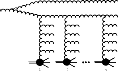
FIG. 4.:

Once we perform the impact parameter integration using a gaussian profile function we obtain

$$xg_{A}(x,Q^{2})=\frac{2R_{A}^{2}}{\pi^{2}}\,\int_{x}^{1}\frac{dx^{\prime}}{x^{\prime}}\,\int_{1/Q^{2}}^{1/Q^{2}_{0}}\frac{d^{2}r_{t}}{\pi r_{t}^{4}}$$ (23)

$$\left[C+\ln(\kappa_{G}(x^{\prime},r_{t}^{2}))+E_{1}(\kappa_{G}(x^{\prime},r_{t}^{2}))\right]\,\,,$$ (24)

where $C$ is the Euler constant, $E_{1}$ is the exponential function and where the $\kappa_{G}$ function was introduced as

$$\kappa_{G}(x,r_{t}^{2})=\frac{3\alpha_{s}}{2R_{A}^{2}}\pi r_{t}^{2}xg(x,1/r_{t}^{2})\,\,.$$ (25)

The expansion of Eq. (18) in terms of $\kappa_{G}$ gives as the Born term the DGLAP equation in the small $x$ region, the higher order terms corresponding to the unitarity corrections naturally implemented in this formalism.

The estimation of the shadowing effect due to gluon recombination can be immediately obtained studing the ratio $R_{1}=xg_{A}(x,Q^{2})/Axg_{N}^{GRV}(x,Q^{2})$ presented in Fig. (5), where we calculate for $Ca$ and $Au$, and analysed the behavior of this function in terms of $\ln(1/x)$, $A^{1/3}$ and $\ln Q^{2}$. We used the GRV parametrization [27] and adapted the calculation in order to have a larger domain of validity in $x$ using

$$xg(x,Q^{2})=xg_{A}[Eq.(18)]+Axg^{GRV}(x,Q^{2})$$ (26)

$$-A\,\frac{\alpha_{s}N_{c}}{\pi}\int_{x}^{1}\int_{Q_{0}^{2}}^{Q^{2}}\frac{dx_{1}}{x_{1}}\frac{dQ^{\prime\,2}}{Q^{\prime\,2}}x^{\prime}g(x^{\prime},Q^{2})\,\,,$$ (27)

where $A\,xg^{GRV}(x,Q_{0}^{2})$ is the initial condition. The same procedure could be applied for another global parametrization based on DGLAP.

As expected the UC increase with $A$, and get smaller as $Q^{2}$ increases and it is evident the importance of the effect as $x$ goes to small values. This allows us to say that the UC should be included in the calculations related with the nuclear gluon distribution function, and the obtained function $xg_{A}(x,Q^{2})$ may be used to set the initial conditions for future experiments. For instance in HERA-A, in processes $e^{\pm}A$ [28] the function $xg_{A}$ could be obtained indirectly and employed as an initial condition for the hadronic high energy processes at RHIC and LHC.

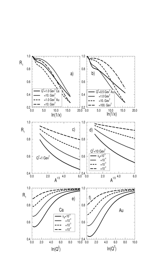
FIG. 5.:

The quarks and gluons distribution were also analysed for the nucleon in this formulation [13], as well as the structure function $F_{2}$ [29]. The motivation for this generalization is the availability of HERA data.

The free interpretation of the Froissart theorem for hadronic processes requires a limit for the increasing of the cross section $\sigma_{\gamma^{*}N}$ and $F_{2}$ with the energy so unitarity is not violated. Concentrating the discussion on the $\kappa$ value, $\kappa=xg(x,Q^{2})\sigma^{gg}/(Q^{2}\pi R^{2})=3\pi\alpha_{s}xg(x,Q^{2})/2Q^{2}R^{2}$, which is the probability of gluons interactions inside the partonic cascade, and $R$ is the radius of the nucleon area occupied by the gluons, we were able to obtain $R^{2}=5$ GeV^-2, and that $\kappa$ reaches 1 at HERA, meaning the effects of shadowing should be considered in the analysis [12, 13, 30]. In the nucleon case, following the same steps as before we obtain

$$xg(x,Q^{2})=\frac{4}{\pi^{2}}\int_{x}^{1}\frac{dx^{\prime}}{x^{\prime}}\int_{4/Q^{2}}^{\infty}\frac{d^{2}r_{t}}{\pi r_{t}^{4}}\int_{0}^{\infty}\frac{d^{2}b_{t}}{\pi}$$ (28)

$$2\,[1-e^{-\frac{1}{2}\sigma_{N}^{gg}(x^{\prime},4/r_{t}^{2})S(b_{t})}]\,\,,$$ (29)

and requiring the recovering of DGLAP at DLA we have

$$\sigma_{N}^{gg}(x,4/r_{t}^{2})=\frac{3\pi^{2}\alpha_{s}}{4}r_{t}^{2}xg(x,4/r_{t}^{2})\,.$$ (30)

For the quarks, considering the scattering of a virtual photon that decays into a quark-antiquark pair, which interacts with the nucleon through the exchange of a ladder we get

$$\sigma(\gamma^{*})=\int_{0}^{1}dz\int d^{2}r_{t}|\Psi(z,r_{t})|^{2}\,\sigma_{tot}^{q\bar{q}+N}\,,$$ (31)

where $\Psi$ is the wavefunction of the $q\bar{q}$ in the virtual photon [26]. We obtain

$$\sigma_{tot}=\int d^{2}b_{t}\,[1-e^{-\frac{1}{2}\Omega_{q\bar{q}}(x,r_{t},b_{t})}]\,.$$ (32)

Here $\Omega_{q\bar{q}}$ is the opacity function that in the Glauber (or eikonal) approach is equivalent to $\Omega=\frac{4\pi^{2}\alpha_{s}(Q^{2})}{3Q^{2}}xg(x,Q^{2})S(b_{t})$. In doing so we are able to reproduce DGLAP evolution for $\Omega<1$, and guarantee the validity of the formulation also for the kinematical region where $\Omega>1$.

Taking $\Omega\rightarrow\infty$ and factorizing the $b_{t}$ dependence we obtain the unitarity limit for the structure function, having for the $\ln Q^{2}$ derivative of $F_{2}$ , $\partial F_{2}/\partial\ln Q^{2}<Q^{2}\,R^{2}/3\pi^{2}$. Using GRV, the unitarity limit for HERA is reached for $Q^{2}=Q^{2}_{0}=1-2$ GeV² ($y=\ln 1/x\sim 9$). Similarly, for gluons it is $Q^{2}=1-2$ GeV² ($y=\ln 1/x\sim 7$) for HERA [30].

With the aim to obtain a non-linear evolution equation containing the unitarity corrections through the inclusion of all the interactions besides the fastest parton from the ladder, we differentiate our master equation for the gluon in $y=\ln 1/x$ and $\varepsilon=\ln Q^{2}$, obtaining

$$\frac{\partial^{2}xg(y,\varepsilon)}{\partial y\partial\varepsilon}=\frac{2\,Q^{2}R^{2}}{\pi}\,[C+\ln(\kappa_{G})+E_{1}(\kappa_{G})]\,,$$ (33)

where $\kappa_{G}^{DGLAP}(x,Q^{2})=\frac{N_{c}\alpha_{s}\pi}{2Q^{2}R^{2}}xg^{DGLAP}(x,Q^{2})$ for calculations.

In terms of $\kappa_{G}$ the main evolution equation is

$$\frac{\partial^{2}\kappa(y,\varepsilon)}{\partial y\partial\varepsilon}+\frac{\partial\kappa(y,\varepsilon)}{\partial y}=\frac{N_{c}\alpha_{s}}{\pi}\,[C+\ln(\kappa_{G})+E_{1}(\kappa_{G})]\,.$$ (34)

It should be mentioned that large distance effects are absorved in the initial condition for the evolution, and situating in a conveninet region of $Q^{2}$ only short distance effects are present, meaning a perturbative calculation is reliable.

Equations (25) and (26) were derived in Ref. [12, 13], and refered for simplicity as AGL equation. The main properties of this formulation are:

• all contributions from the diagrams of order $(\alpha_{s}y\varepsilon)^{2}$ are resummed;

• in the limit $\kappa\rightarrow 0$ the DGLAP evolution in DLA is fully recovered;

• for $\kappa<1$, and not large, the GLR equation is recovered;

• for $\alpha_{s}y\varepsilon\approx 1$ the equation is equivalent to the Glauber formalism.

The UC are described for the different kinematical regions of $\kappa$ from strictly perturbative QCD up to the onset of hdQCD. Non-perturbative effects are not explicitly described and this is the object of a distinct formalism $MV-JLKM$ [10] that we will briefly comment in a next subsection. In Fig. (6) the comparison between the solutions of the equations AGL, GLR, DGLAP and Glauber-Mueller (MOD MF) formula is presented, where the control of the growing of the gluon distribution once UC are considered is very evident.

It was also obtained the asymptotic solution $\kappa>1$ of the AGL equation for fixed $\alpha_{s}$ [12, 13] as well as for running $\alpha_{s}$ [31]. For high partonic density and $y>>y_{0}$ we obtain

$$\kappa_{G}^{asymp}(y)=\frac{\alpha_{s}N_{c}}{\pi}\,y\ln y\approx\frac{\alpha_{s}N_{c}}{\pi}y\,.$$ (35)

FIG. 6.:

This solution is a good approximation for very small values of $x$ (${\cal O}(10^{-8})$), related with THERA physics [28], region of a very dense parton system. In terms of the gluon function the asymptotic behavior is

$$xg(x,Q^{2})=\frac{2\,N_{c}Q^{2}R^{2}}{3\,\pi^{2}}\/\ln(1/x)\,,$$ (36)

presenting a behavior softer than predicted by DGLAP, meaning a partial saturation.

For the running $\alpha_{s}$ the result is [31]

$$xg(x,Q^{2})=\frac{\varepsilon}{1+\varepsilon}\,\frac{2N_{c}Q^{2}R^{2}}{3\pi^{2}}\ln(1/x)\,.$$ (37)

where $\varepsilon=\ln Q^{2}/\Lambda_{QCD}^{2}$. The partial saturation is not modified, and the main difference from the previous result occours for small values of $\varepsilon$. This confirms the expectation that the UC are already relevant before the corrections to leading order [30, 32].

C The Kovchegov Formulation

The unitarization problem in QCD was addressed as an extension of the dipoles formalism for the BFKL equation by Kovchegov [11]. This work proposes a non linear generalization of BFKL equation, also addressed previously in Ref. [33] by the use of OPE to QCD obtaining the evolution of Wilson line operators. The scattering of a dipole (onium - $q\bar{q}$) with the nucleon is described by a cascade evolution corresponding to the successive subdivision of dipoles from the father dipole. Each dipole has multiple scatterings with the nucleons of the target, implying multiple ladders exchange to be resummed in order to obtain the cross section of the interaction of the dipole with the nucleus. As a result it is derived the evolution equation having the unitarized BFKL Pomeron as solution, in the LL($1/x$) approximation.

The scattering of the onium $q\bar{q}$ (dipole) with the nucleus in the rest frame, takes place through a cascade of soft gluons, which once taken in the $N_{c}\rightarrow\infty$ limit is simplified by the suppression of non-planar diagrams. The gluons are replaced by $q\bar{q}$ pairs and the dipole Mueller’s technique for the perturbative cascade can be employed [34].

The Kovchegov formulation, as the AGL, is a perturbative QCD calculation and the considered dipoles from the cascade interact independently with the nucleus. The onium-onium frontal scattering has the cross section $\sigma=-2\,{\cal I}m{\cal A}$, where the amplitude

$${\cal A}=-i\int d^{2}x\int_{0}^{1}dz\int d^{2}x_{1}\int_{0}^{1}dz_{1}\,\Phi(\vec{x},z)\,F\,\Phi(\vec{x_{1}},z_{1})\,,$$ (38)

where $\Phi(\vec{x},z)$ is the square of the onium wave function, $\vec{x}$ is the transverse separation of the $q\bar{q}$ pair, and $z$ is the longitudinal fraction of momentum of the quark. For the exchange of only two gluons, without gluon ladder evolution the function $F$ is [26]

$$F^{(0)}(\vec{x},\vec{x_{1}})=-\frac{\pi\alpha^{2}_{s}(N_{c}^{2}-1)}{N_{c}^{2}}x^{2}_{<}\,(1+\ln(\frac{x_{>}}{x_{<}}))\,,$$ (39)

where $x_{>}(x_{<})$ is the biggest (smaller) between $|\vec{x}|$ and $|\vec{x_{1}}|$. The two gluons approximation is energy independent, but for high energy the contributions of order $(\alpha_{s}Y)^{n}$ should be included ($Y=\ln s/M^{2}$ is the rapidity and $M$ is the onium mass), since they generate the perturbative cascade evolution. The dipole approximation introduces an arbitrary number of soft gluons in the square of the onia wave function $\Phi$, and keeping $F$ as an exchange of two gluons avoids to deal with the reggeization of the gluons and the effective vertex. The transverse coordinates of the quark and antiquark of an ultrarelativistic onium state in $+$ direction are $\vec{x_{0}}=0$ and $\vec{x}$, and successively in the evolution the next emitted gluon should be softer. We have $p-k$ and $k$, as the momenta for the pair, and $z_{1}=\frac{k_{1}^{+}}{p^{+}}$ (in light-cone variables [35]), having as wave function

$$\Psi^{(0)}(x_{01},z_{1})=\int\frac{d^{2}k_{1}}{(2\pi)^{2}}\,e^{i\vec{k_{1}}\vec{x_{01}}}\Psi^{(0)}(k_{1},z_{1})\,,$$ (40)

where $\vec{x_{01}}=\vec{x_{1}}-\vec{x_{0}}$, and $\Phi^{(0)}=|\Psi^{(0)}|^{2}$, keeping factorization in this procedure. This allows to obtain the dipole density, $n$, considering $x_{02}>\rho,\,x_{12}>\rho$, where $\rho$ is an ultraviolet cut also implied by $C$ in the expression below

$$n (x_{01},x,Y)=x\delta(x-x_{01})\exp\left[-\frac{2\alpha_{s}N_{c}}{\pi}\,Y\,\ln(\frac{x_{01}}{\rho})\right]$$ (41)

$$+ \frac{\alpha_{s}N_{c}}{\pi^{2}}\int_{C}\frac{x_{01}^{2}\,d^{2}x_{2}}{x_{02}^{2}\,x_{12}^{2}}\,\int_{0}^{Y}dy\exp\left[-\frac{2\alpha_{s}N_{c}}{\pi}(Y-y)\,\ln(\frac{x_{01}}{\rho})\right]$$ (42)

$$\times n(x_{12},x,y)\,,$$ (43)

for $Y=\ln s/M^{2}$, which is represented in Fig. (7).

FIG. 7.:

The next step is to obtain an evolution equation for the dipole density assuming the propagation of the dipoles in the target is represented by the function $\gamma_{1}(\vec{x},\vec{b})$, where $b$ is the impact parameter, and which should be added to the density $n_{2}$, equally convoluted with $\gamma_{2}(\vec{x_{1}},\vec{b_{1}},\vec{x_{2}},\vec{b_{2}})$, etc. Assuming no correlation among the dipoles $\gamma_{n}(...)=\gamma_{1}(\vec{x_{1}},\vec{b_{1}})...\gamma_{1}(\vec{x_{n}},\vec{b_{n}})$, the cross section for the interaction onium nucleus $N(\vec{x_{01}},\vec{b_{0}},Y)$ is then given by [11]

$$-N(\vec{x_{01}},\vec{b_{0}},Y)=\sum_{i}^{\infty}\int n_{i}(x_{01},Y,\vec{b_{1}},\vec{x_{1}},...,\vec{b_{i}},\vec{x_{i}})$$ (44)

$$\times\left[\gamma(\vec{x_{1}},\vec{b_{1}})\frac{d^{2}x_{1}}{2\pi x_{1}^{2}}d^{2}b_{1}\right]...\left[\gamma(\vec{x_{i}},\vec{b_{i}})\frac{d^{2}x_{i}}{2\pi x_{i}^{2}}d^{2}b_{i}\right]$$ (45)

Finally, omitting some steps of the calculation [11] the evolution equation for $N(\vec{x_{01}},\vec{b_{0}},Y)$ is

$$N(\vec{x_{01}},\vec{b_{0}},Y)=-\gamma(\vec{x_{01}},\vec{b_{0}})\exp\left[-\frac{4\alpha_{s}C_{F}}{\pi}\ln(\frac{x_{01}}{\rho})Y\right]+$$ (46)

$$\frac{\alpha_{s}C_{F}}{\pi^{2}}\int_{0}^{Y}dy\exp\left[-\frac{4\alpha_{s}C_{F}}{\pi}\ln(\frac{x_{01}}{\rho})(Y-y)\right]\,\times$$ (47)

$$\times\int_{\rho}d^{2}x_{2}\frac{x_{01}^{2}}{x_{02}^{2}x_{12}^{2}}\,\left[\,2N(\vec{x_{02}},\vec{b_{0}}+\frac{1}{2}\vec{x_{12}},y)\right.-$$ (48)

$$\,-\,\left.N(\vec{x_{02}},\vec{b_{0}}+\frac{1}{2}\vec{x_{12}},y)N(\vec{x_{12}},\vec{b_{0}}-\frac{1}{2}\vec{x_{20}},y)\right]\,,$$ (49)

where $x_{ij}=x_{i}-x_{j}$, the size of the dipole whose quark has transverse coordinate $x_{i}$, and the antiquark $x_{j}$, $\gamma(\vec{x_{01}},\vec{b_{0}})$ is the propagator of the pair $q\bar{q}$ through the nucleus, describing the multiple rescattering of the dipole with the nucleons within the nucleus. We denote this equation as the $K$ equation.

The physical representation is comparable with the approach Glauber-Mueller since the incident photon generates a $q\bar{q}$ that subsequently emits a gluon cascade further interacting with the nucleus. At large $N_{c}$ limit the gluon can be represented by a $q\bar{q}$ pair, and we can expect in this limit and DLA that the gluon cascade could be interpreted as a dipole cascade. Although beguinning the formulations with distinct degrees of freedom both $K$ and AGL resum the multiple rescatterings in their respectives degrees of freedom, which allows to consider they should coincide in a suitable common kinematical limit, which we will show later on.

In DLA, where the photon scale of momentum $Q^{2}$ is bigger than $\Lambda_{QCD}^{2}$, the $K$ equation simplifies to

$$\frac{\partial N(\vec{x_{01}},\vec{b_{0}},Y)}{\partial Y}=\frac{\alpha_{s}C_{F}}{\pi}x_{01}^{2}\,\int_{x_{01}^{2}}^{1/\Lambda_{QCD}^{2}}\frac{d^{2}x_{02}}{(x^{2}_{02})^{2}}\,$$ (50)

$$\times\left[2\,N(\vec{x_{02}},\vec{b_{0}},Y)-N(\vec{x_{02}},\vec{b_{0}},Y)\,N(\vec{x_{02}},\vec{b_{0}},Y)\right]\,,$$ (51)

which is the evolution in transverse size of the dipoles from $x_{01}$ up to $1/\Lambda_{QCD}$. Now deriving in $\ln(1/x_{01}^{2}\,\Lambda_{QCD}^{2})$ results

$$\frac{\partial^{2}N(\vec{x_{01}},\vec{b_{0}},Y)}{\partial Y\partial\ln(1/x_{01}^{2}\,\Lambda_{QCD}^{2})}=\frac{\alpha_{s}C_{F}}{\pi}\,\left[2-N(\vec{x_{01}},\vec{b_{0}},Y)\right]$$ (52)

$$\times N(\vec{x_{01}},\vec{b_{0}},Y)\,.$$ (53)

setting that the successive emission of dipoles generates larger transverse size for each higher generation.

The linear term reproduces BFKL at low density, and the quadratic term introduces UC unitaryzing the BFKL Pomeron and the equation reproduces GLR once we assume $N$ directly related to the gluon distribution function.

D The MV-JKWL Formulation

In the MV-JKWL formulation [10, 36] a very dense system is treated in the light-cone and considering the light-cone gauge ($A^{+}\equiv 0$), $x\equiv q^{+}_{Gluon}/Q^{+}_{Nucleon}$. In Ref. [10] the gluons distribution for small $x$ is proposed for a large nucleus where the degrees of freedom are virtual quanta from a classical field generated by the color charge of the valence partons (static sources). The approach is originally non-perturbative and the nucleus is considered in the infinite momentum frame, transfering the scale of the problem to $\Lambda=1/\pi R^{2}\,dN/dy$, where $N$ is the density of gluons. For small $x$ and a large nucleus $\alpha_{s}(\Lambda)$ is small allowing some perturbative calculation in this effective lagrangian formulation for gluons condensates.

The density of gluons in momentum space is obtained in terms of the correlation of the gluons fields, in the light cone gauge. The intrinsic quantum fluctuations are replaced by a classical average on the color charge ensemble. The gluons distributions at a given virtuality $Q^{2}$ and $x$ is obtained from the density of gluons in the momenta space $dN/dq^{+}q^{2}\vec{q}$, which is a function of the gluon condensate $<A_{i}^{a}(x^{-},\vec{x})\,A(x^{\prime},\vec{x^{\prime}})>$, being

$$xg(x,Q^{2})\equiv\int^{Q^{2}}d^{2}\vec{q}\,x\,\frac{dN}{dxq^{2}\vec{q}}\,.$$ (54)

The gluons distributions, in this framework where a large number of color charges generates a QCD vector potential, is obtained in lowest order by solving the classical Yang-Mills equations, $D_{\mu}\,F^{\mu\nu}=j^{\nu}$.

Introducing a regulator in the valence partons current singularity by considering the color density $\rho$ a function of rapidity, it was obtained [39] an analytical solution for the classical correlations, with the property that for high transverse momentum the classical gluons distribution obeys the Weizsacker-Williams form, and has its behavior softened as $\ln(k_{t}^{2}/\chi(y,k_{t}^{2}))$. Here $\chi=\int_{y}^{\infty}\mu^{2}(y,Q^{2})$ is the squared color charge per unity of area for rapidity bigger than $y$.

In the classical MV the non-linear effects are included in the charge density $\rho$ solution of Y-M equations. The quantum corrections are to be considered, and from Ref. [37] the perturbative result for the gluons distribution up to second order in $\alpha_{s}$ is given by

$$\frac{1}{\pi R^{2}}\frac{dN}{dxd^{2}k_{t}}=\alpha_{s}\Gamma\frac{1}{xk_{t}^{2}}\left[1+\frac{2\alpha_{s}N_{c}}{\pi}\ln(\frac{k_{t}}{\alpha_{s}\mu})\ln(\frac{1}{x})\right]\,,$$ (55)

where $\Gamma=\frac{\mu^{2}(N_{c}^{2}-1)}{\pi^{2}}$ and $\mu^{2}$ is the square of the color charge average density (per unity of area). The additional effect of including the hard gluon was treated in Ref. [38], resulting in the low density limit the BFKL equation, and for high virtualities the DGLAP equation. For high density a complete solution was not yet obtained. In Ref. [40] JKLW analysed their evolution equation in DLA obtaining a generalization of GLR.

As a summary of the formulations for hdQCD at present, the Fig. (8) presents their different regions of applicability as fas as $\kappa$ in concerned in the $\ln(1/x)$ versus $Q^{2}$ plane.

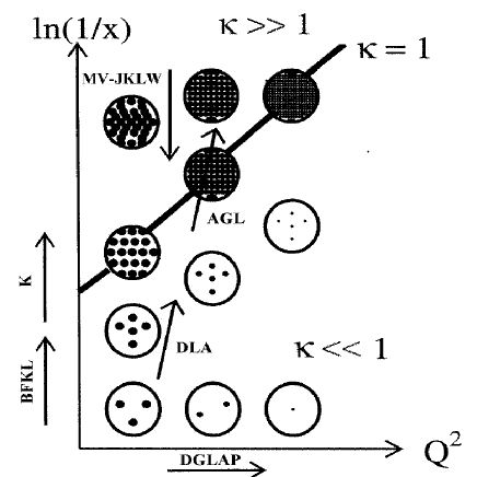
FIG. 8.:

The main questions at this point can be:

• which is the most suitable form to introduce the UC ?

• can we relate the distinct formulations in a common limit analytically ?

• what do we look at the observables as a signature for the UC ?

The last two questions, I will briefly address in the rest of this presentation following our personal contributions to this investigation.

V Connection Among the Formulations

The AGL equation was originally obtained from the Glauber-Mueller approach, but it can be also derived from the dipole representation [41]. We obtained the cross section for the virtual probe $G^{*}$ with the nucleus $\sigma^{G^{*}A}=\int_{0}^{1}dz\int\frac{d^{2}r_{t}}{\pi}|\Psi_{t}^{G^{*}}|^{2}\sigma^{gg+A}$, that can be expressed by means of the dipoles $q\bar{q}$ once we remind $\sigma^{gg+A}=(C_{A}/C_{F})\sigma^{q\bar{q}+A}$. Now in order to estimate the UC the rescatterings of the $q\bar{q}$ pair into the nucleus should be considered, having in mind that [30] $\sigma_{N}^{q\bar{q}}=\frac{C_{F}}{C_{A}}(3\alpha_{s}(4/r_{t}^{2})/4)\pi^{2}r_{t}^{2}xg_{N}(x,4/r_{t}^{2})$, where $xg_{N}$ is the nucleon gluon distribution. The wave function $\Psi^{G^{*}}$ calculated in [26, 30] is such that $|\Psi_{t}^{G^{*}}|^{2}=\frac{1}{z(1-z)}[(\epsilon^{2}K_{0}(\epsilon t_{t})-\epsilon K_{1}(\epsilon r_{t})/r_{t})^{2}+1/r_{t}(\epsilon K_{1}(\epsilon r_{t}))^{2}]$, where $\epsilon^{2}=Q^{2}z(1-z)$, and the $K_{i}$ are the modified Bessel functions. For small $z$ and $\epsilon r_{t}<<1$ we obtain

$$xg_{A}(x,Q^{2})= \frac{4}{\pi}\,\frac{C_{A}}{C_{F}}\int_{x}^{1}\frac{dx^{\prime}}{x^{\prime}}\int_{4/Q^{2}}^{\infty}\frac{d^{2}r_{t}}{\pi r_{t}^{4}}$$ (56)

$$\times 2\,\left[\,1-e^{-\frac{1}{2}\sigma_{N}^{q\bar{q}}S(b_{t})}\,\right]\,.$$ (57)

From this equation we can obtain the AGL equation in the dipole representation by differentiating in $y=\ln 1/x$ and $\ln Q^{2}/\Lambda_{QCD}^{2}$ having

$$\frac{\partial^{2}xg(x,Q^{2})}{\partial y\,\,\partial\ln Q^{2}/\Lambda_{QCD}^{2}}=C^{\prime}Q^{2}\int\frac{d^{2}b_{t}}{\pi}\left[1-e^{-\frac{1}{2}\sigma_{N}^{q\bar{q}}S(b_{t})}\right]\,,$$ (58)

valid in DLA, considering each gluon of the cascade as a $q\bar{q}$ in the high $N_{c}$ limit, and where $C^{\prime}=2C_{A}/\pi^{2}C_{F}$. For a central collision and $S_{\perp}=\pi R^{2}$, and $S(0)=A/\pi R^{2}$

$$\frac{\partial^{2}xg(x,Q^{2})}{\partial y\,\partial\ln Q^{2}/\Lambda_{QCD}^{2}}=DQ^{2}\left[1-e^{-\frac{2\alpha_{s}\pi^{2}}{N_{c}S_{\perp}Q^{2}}xg_{A}}\right]\,,$$ (59)

for $N_{c}=3$, $C_{F}=N_{c}/2$ at high $N_{c}$, and where $D=\frac{N_{c}C_{F}S_{\perp}}{\pi^{3}}$.

The GLR for a cylindrical nucleus is immediately obtained from Eq. (59) by its expansion up to second order in $xg_{A}$. Again, for small UC only the first term contributes which reproduces DGLAP in the DLA limit. Those results are in Ref. [41]

Now, the Eq. (34) is the K equation that in DLA, where the scale of momentum of the photon $Q^{2}$ is higher than the scale of momentum of the nucleus $\Lambda^{2}_{QCD}$, simplifies as

$$\frac{\partial N(\vec{x_{01}},\vec{b_{0}},Y)}{\partial Y}=\frac{\alpha_{s}C_{F}}{\pi}x_{01}^{2}\int_{x_{01}^{2}}^{1/\Lambda^{2}_{QCD}}\frac{dx_{02}^{2}}{(x_{02}^{2})^{2}}$$ (60)

$$\times\left[2N(\vec{x_{02}},\vec{b_{0}},Y)-N^{2}(\vec{x_{02}},\vec{b_{0}},Y)\right]\,.$$ (61)

This equation considers the evolution of the dipoles from $x_{01}$ up to $1/\Lambda_{QCD}$ in the transverse direction. Now deriving Eq. (61) in $\ln(1/(x_{01}^{2}\Lambda^{2}_{QCD}))$ we get

$$\frac{\partial^{2}N(\vec{x_{01}},\vec{b_{0}},Y)}{\partial Y\partial\ln(1/x_{01}^{2}\Lambda^{2}_{QCD})}=\frac{\alpha_{s}C_{F}}{\pi}\left[\ 2-N\,\right]N\,.$$ (62)

We should relate now the function $N(\vec{x}_{01},\vec{b_{0}},Y)$ with the gluon distribution function. For that we consider the structure function $F_{2}$ for the nucleus as obtained in [11], following [25], and analized in [29] for $b_{t}=0$, which is

$$F_{2}^{A}(x,Q^{2})=\frac{Q^{2}}{4\pi^{2}\alpha_{em}}R^{2}\int dz\int\frac{d^{2}r_{t}}{\pi}|\Psi|^{2}$$ (63)

$$\times 2\left[1-e^{-\frac{\alpha_{s}C_{F}\pi^{2}}{N_{c}^{2}S_{\perp}}r_{t}^{2}Axg(x,1/r_{t}^{2})}\right]\,.$$ (64)

This estimates the UC for the nuclear structure function, for central collisions in the DLA limit in the Glauber-Mueller approach.

Considering the unitarity corrections due to the multiple rescattering of the $q\bar{q}$ pairs with the distinct nucleons into the nucleus, from the just obtained expression for $F_{2}^{A}$, it results the relation

$$N(\vec{x_{01}},\vec{b_{0}}=0,Y)=2\left[1-e^{\frac{-2\alpha_{s}C_{F}\pi^{2}}{N_{c}^{2}S_{\perp}}x_{01}^{2}Axg(x,1/x_{01}^{2})}\right]\,,$$ (65)

where $x_{01}=x_{0}-x_{1}=r_{t}$, $Y=\ln(s/Q^{2})=\ln(1/x)$ establishing a connection between the cross-section of the $q\bar{q}$ pair and the gluon structure function in DLA limit.

We are in good terms to verify the connection among the K and AGL formulations since we already obtained the AGL equation in the dipole formulation, Eq. (40), the K equation in the DLA limit, Eq. (42), the cross section of the pair through the dipole density from K and the nuclear gluon distribution function, Eq. (45).

Having Eq. (45) in Eq. (41) and for $x_{01}\approx 2/Q$, as in [10], we obtain

$$\frac{\partial^{2}xg_{A}(x,Q^{2})}{\partial y\partial\ln(Q^{2}/\Lambda_{QCD}^{2})}=D\,Q^{2}\left[1-e^{-\frac{2\alpha_{s}\pi^{2}}{N_{c}s_{\perp}Q^{2}}xg_{a}}\right]\,,$$ (66)

result already obtained, and that gives GLR as a limit.

Our comparison has physical meaning for dipoles with small transverse sizes and for the above connection among $N$ and $xg_{A}$ [Eq. (45)].

In Refs. [38, 39] it was applied the Wilson renormalization group to the model of McLerran and Venugopalan. The non-linear evolution equation then obtained deals with the weight function of the color charge densities, valid at leading order $\alpha_{s}$ and for densities up to $1/\alpha_{s}$. The complete analytical solution is not yet obtained but some limits are discussed. At low densities BFKL is recovered, and then at DLA at large $Q^{2}$ DGLAP is recovered. In the work [40] is proposed the equation

$$\frac{\partial^{2}xg(x,Q^{2},b_{t})}{\partial y\partial\varepsilon}=\beta\,Q^{2}\left[1-\frac{1}{x}exp(1/\kappa)E_{1}(1/\kappa)\right]\,,$$ (67)

where $\beta=N_{c}(N_{c}-1)/2$ and $\kappa(x,Q^{2},b_{t})=2\alpha_{s}/\pi(N_{c}-1)Q^{2}xg(x,Q^{2},b_{t})$.

For large $\kappa$, a factorized $b_{t}$ dependence and considering a central collision we obtain for this equation

$$\frac{\partial^{2}xg(x,Q^{2})}{\partial y\partial\varepsilon}=\beta R^{2}Q^{2}\,,$$ (68)

which solution is

$$xg(x,Q^{2})=\beta\pi R^{2}Q^{2}\ln(1/x)\,,$$ (69)

presenting the same $Q^{2}$ and $x$ behavior as the asymptotic solution for AGL. The main point is the partial saturation of the gluon distribution presented in both formulations in the asymptotic region. A connection among those two formulations in a more broad kinematical region is still an open question.

The asymptotic behavior of the structure function also required our attention. Considering the relation of $\sigma^{q\bar{q}}$ and $xg(x,Q^{2})$ we can write [29]

$$F_{2}(x,Q^{2})=\frac{2\alpha_{s}}{9\pi}\int_{Q_{0}^{2}}^{Q^{2}}\frac{dQ^{2}}{Q^{2}}xg(x,Q^{2})$$ (70)

which is a leading twist equation, with limited application for high densities, due to higher twist terms related with the UC.

Using the solution of AGL in the asymptotic regime as input in the above equation we obtain $F_{2}(x,Q^{2})\simeq\frac{\alpha_{s}}{\pi^{3}}R^{2}Q^{2}\ln(1/x)$, which again presents partial saturation, meaning the Froissart limit is not violated [44]. Analogous result was obtained by Kovchegov [42] employing the solution of the K equation [11]. We obtained that the asymptotic behavior of $F_{2}$ is a general characteristic that appears to be independent from the approach that is used [31].

Assuming the asymptotic behavior of the gluon function is $xg(x,Q^{2})=2Q^{2}R^{2}/3\pi\alpha_{s}$, it implies saturation for $F_{2}$ ($\sim R^{2}Q^{2}$) for very small $x$. However this result should be taken with caution since it is valid in a kinematical region where higher order in the partonic density are not significative. The subject of saturation is a tricky one and it seems we are far from establishing its features in a solid theoretical basis [24]. Important contributions to these challenging aspects of hdQCD are to be found in Mueller [24] for the theoretical discussion and Golec-Biernat and Wüsthoff [24] for a phenomenological application.

In [43, 44] we were able to show that

$$F_{2}(x,Q^{2})=\frac{R^{2}}{2\pi^{2}}\sum_{i}e_{i}^{2}\int_{1/Q^{2}}^{1/Q_{0}^{2}}\frac{d^{2}r_{t}}{\pi r_{t}^{4}}\left[C+\ln\kappa_{q}+E_{1}(\kappa_{q})\right]\,,$$ (71)

where $\kappa_{q}=4/9\kappa_{g}$. From that we can estimate the UC for $F_{2}$ in the DLA limit. For large $\kappa_{q}$, and using the asymptotic solution of AGL, we obtained [31]

$$F_{2}(x,Q^{2})\simeq\frac{R^{2}Q^{2}}{3\pi^{2}}\ln[\frac{4\alpha_{s}}{3}\ln(1/x)]\,,$$ (73)

when higher twist terms are considered in $F_{2}$. This is a softer behavior, but in both cases there is no violation of the Froissart limit. This above equation was not studied in K or MV-JKLW approaches.

From the already obtained results it follows the identity [45]

$$\frac{\partial F_{2}(x,Q^{2})}{\partial\ln Q^{2}}=F_{2}(x,Q^{2})\,,$$ (74)

as an important signature of the asymptotic regime of QCD for dense systems. It is relevant to mention that for the same center of mass energy this regime is reached for nucleus for smaller partonic densities than in the nucleon case, since $\kappa_{A}=A^{1/3}\kappa_{N}$.

VI Phenomenology

From the Glauber-Mueller formalism for high dense partonic systems was demonstrated the AGL equation and its asymptotic behavior. It was also obtained the nucleon and the nuclear gluon distribution function as well as the respective structure functions and derivatives. This formulation incorporates the UC required by the Froissart bound, through a non linear dynamics.

In this section the behavior of the main observables obtained in $ep$ collisions, and relevant for $eA$ collisions, will be analysed with the goal to shed some light in the subject of UC.

For $ep$ we studied the behavior of the proton structure function $F_{2}$, its derivative $\frac{\partial F_{2}}{\partial\ln Q^{2}}$, the charmed component of the structure function $F_{2}^{c}$, and the longitudinal distribution function, $F_{L}$ [43].

There is a large amount of data from HERA to motivate a detailed study of these observables directly connected with the gluon distribution function. As previously demonstrated the gluon distribution is modified in a unitarity corrected formulation, meaning those observables should be affected.

We were lucky to show that the $\frac{\partial F_{2}}{\partial\ln Q^{2}}$, the $F_{2}^{c}$ are clearly modified. Also, the $eA$ analysis provides stricking results for the nuclear structure function $F_{2}^{A}$ and its derivative, as an important signature of the UC corrections. These results are important since they are a prediction both for HERA-A and for $e$-RHIC, in which a high dense parton system should be formed.

The increasing of $F_{2}$ in HERA in the small $x$ region ($10^{-2}>x>10^{-5}$) is observed even for small virtualities ($Q^{2}\approx 1$ GeV²). Taking $F_{2}\sim x^{-\lambda}$, for small $x$ data is compatible with $\lambda=0.15$ ($Q^{2}=0.85$ GeV²) up to $\lambda=0.4$ ($Q^{2}=20$ GeV²). This is described by DGLAP with suitable input initial condition for $Q^{2}$ and distributions by different groups [27, 47]. It will conduct to the idea UC are not observable in the HERA kinematical range. We have shown that the structure function is too inclusive in the gluon function to clearly explicitate the UC.

We arrived at a different conclusion applying AGL to $\frac{\partial F_{2}}{\partial\ln Q^{2}}$, $F_{L}$ and $F_{2}^{c}$, all observables directly associated with the gluon function.

The derivative of $F_{2}$ is

$$\frac{\partial F_{2}}{\partial\ln Q^{2}}=\frac{R^{2}Q^{2}}{2\pi^{2}}\sum_{i}e^{2}_{i}[\,C+\ln(\kappa_{q})+E_{1}(\kappa_{q})\,]\,,$$ (75)

that we solved using the same procedure as Eq. (20). The usual parametrizations [27, 47] do not include the UC for the gluons explicitly. We use Eq. (20) for $A=1$ as input, and we obtain the corrections from both sectors quark and gluons. The last one gains in importance as $Q^{2}$ increases. In Fig. (9) the results for $\frac{\partial F_{2}}{\partial\ln Q^{2}}$ are presented for $R^{2}=5$ GeV². For the complete discussion we refer to [48]. The UC for both sectors are able to describe properly the data including the turn-over. Our conclusions is this is a good observable to evidentiate the presence of the UC. This question was addressed also in [49] calculating the suppression factors separately.

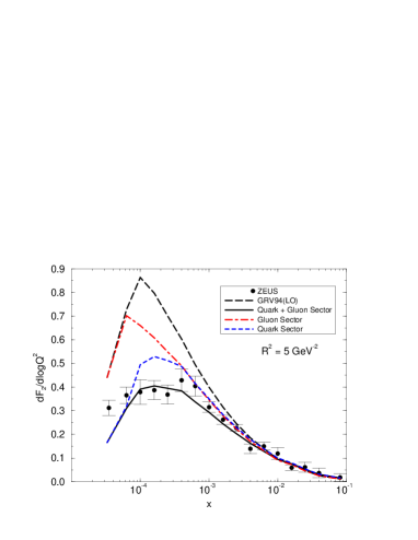
FIG. 9.:

We believe that the UC should be extracted from data related to observables that are directly dependent of the gluon function. The longitudinal structure function $F_{L}$ is a difficult measurement requiring distinct values of the center of mass energy, meaning different energy beams. An alternative is to consider the radiation of a hard photon from the incident electron, reducing the center of mass energy. If this should be done we can study $F_{L}(x,Q^{2})$ in the small $x$ region [43].

Expressed considering the quarks transverse momenta due to gluon radiation, the longitudinal structure function reads

$$F_{L}(x,Q^{2})=\frac{\alpha_{s}(Q^{2})}{2\pi}x^{2}\,\int_{x}^{1}\frac{dy}{y^{3}}\left[\frac{8}{3}F_{2}(y,Q^{2})\right.$$ (76)

$$\left.+\,4\,\sum_{f}e_{f}^{2}(1-\frac{x}{y})yg(y,Q^{2})\right]\,,$$ (77)

where $y=Q^{2}/sx$ and the dependence on the gluon distribution is explicit, meaning this function should be sensitive to unitarity corrections in HERA kinematical region. Our results for small $x$ region are in Fig. (10) [43] compared with the H1 data [50]. Although it seems to be a good observable to evidentiate the UC the available data do not allow any definite conclusion for now.

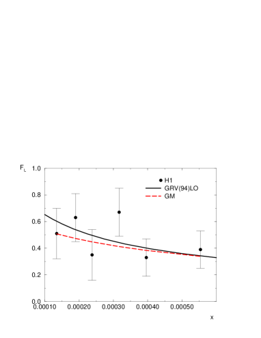
FIG. 10.:

A problably more promissing observable is the rate $R_{F}=F_{2}^{c}(x,Q^{2})/F_{2}(x,Q^{2})$, where $F_{2}^{c}$ is the charmed component of the structure function. Considering the approach of boson-gluon in order to create the $c\bar{c}$ pair we obtained in the Glauber-Mueller formalism the ratio $R_{F}$.

This ratio is presented in Fig. (11) [43] as a function of $\ln(1/x)$. There is strong modification of the ratio once UC are included in the calculation. We urge data in this observable. The suppression is much stronger than in the $F_{2}$ case, and we expect a lower production of quark charm for small $x$, and this is related with the production of $J/\Psi$ which is proportional to the square of the gluon function.

FIG. 11.:

Finally, one of our most stricking results concerns $eA$ physics, and is related with the high dense partonic system in the nuclear medium. The nuclear shadowing is a challenge for hdQCD and mainly important for HERA-A, RHIC and LHC physics. We estimated how the nuclear structure function and its derivative are modified by the effects of high partonic densitiy.

The shadowing corrections to $F_{2}^{A}$ are associated to the rescatterings of the $q\bar{q}$ in the nucleons into the nucleus, being dependent on the nucleon gluon distribution function. Here also we separate the two cases: quark sector, where the gluon distribution is not modified by UC, and quark + gluon sector, where now the gluon distribution is modified a la Glauber-Mueller. The results are presented in Fig. (12) [51] as a ratio $R_{1}=F_{2}^{A}/AF_{2}^{N}$, showing that for small $x$ the gluon sector contribution should be included, and promote saturation.

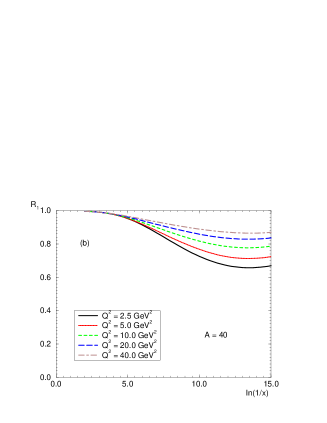
FIG. 12.:

We obtain that the suppression due to the shadowing in $F_{2}^{A}$ is proportionally smaller than in $xg_{A}$ in a perturbative framework, in a different result that in [19] where soft physics is the main issue. As a new result the saturation of the ratio is attained at HERA-A region when the gluon sector is included. The presence of saturation in the perturbative region ($Q^{2}>1$ GeV²) denotes the large shadowing corrections in the gluon sector.

The analysis was extended to the derivative of the nuclear structure function

$$\frac{\partial F_{2}^{A}}{\partial\log Q^{2}}\frac{R^{2}_{A}Q^{2}}{2\pi^{2}}\sum_{i}e_{i}^{2}\left[C+\ln(\kappa_{q})+E_{1}(\kappa_{q})\right]\,,$$ (78)

considering the contributions of the quark and the gluon sectors to the UC. for HERA-A $s=9.10^{4}$ GeV².

The predictions are in Fig. (13) [52] compared with a DGLAP calculation with GRV without nuclear effect. The expected turn-over is present in the orthodox calculation but it is $A$ independent. The behavior of the derivative is different once UC are considered since the maximum is $A$ dependent and runs to higher values of $x$ and $Q^{2}$ as $A$ increases. We conclude this is the best quantity to look for unitarity corrections, evidentiating the same partonic density is reached as $A$ increases for higher values of $x$ and higher values of $Q^{2}$, corroborating a perturbative calculation.

This is a strong motivation to develop this calculation for heavy ion physics, and try to connect this formulation with the research in $AA$ physics where the quark-gluon plasma is expected to be produced.

FIG. 13.:

VII Outlook

Several aspects of the formulations for hdQCD and in our approach to the subject as well require further investigation. I understand the formulation of high dense partonic system should incorporate the methods of nonperturbative physics and non-linear dynamics in order to present a comprehensive formulation for a large kinematical regime in $x$ and $Q^{2}$, besides incorporating the $A$ dependence. However significative progress in the description of hdQCD has been made in the recent years towards a unified theoretical framework. Particularlly relevant is the role of initial conditions for UC for the perturbative treatments and the determination of saturation region, $Q_{s}^{2}$, still to be obtained analytically. Also a complete solution of the generalized evolution equation (Eq. (26)) for $\alpha_{s}(Q^{2})$ outside the asymptotic region is not available. Reaching these goals will allow us to have a more complete dynamical description of the non-linear phenomena of transition between large distance and short distance physics promoting QCD to a more understandable and applicable theory.

REFERENCES

- [1] A. M. Cooper-Sarkar, R.C.E. Devenish and A. De Roeck, Int. J. Mod. Phys A13, 3385 (1998); H. Abramowicz, A. Caldwell, Rev. Mod. Phys. 71, 1275 (1999).
- [2] C. Pajares, Acta Phys. Polon. B30, 2263 (1999).
- [3] S. Tapprogge, Nucl. Phys. (Proc.Suppl.) B86, 150 (2000).
- [4] ZEUS collaboration, M. Derrick et. al., Zeit. Phys. C65, 379 (1995); H1 collaboration, T. Ahmed et. al., Nucl. Phys. B439, 471 (1995); H1 collaboration, S. Aid et al., Nucl. Phys. B470, 3 (1996).
- [5] R. D. Field, Applications of Perturbative QCD, Addison Wesley, New York, 1989.
- [6] V. N. Gribov and L. N. Lipatov, Sov. Journ. Nucl. Phys. 15, 438 (1972); Yu. L. Dokshitzer, Sov. Phys. JETP 46, 641 (1977); G. Altarelli and G. Parisi, Nucl. Phys. B126, 298(1977).
- [7] E.A. Kuraev, L.N. Lipatov and V.S. Fadin, Phys. Lett B60, 50 (1975); Sov. Phys. JETP 44, 443 (1976); Sov. Phys. JETP 45, 199 (1977); Ya. Balitsky and L.N. Lipatov, Sov. J. Nucl. Phys. 28, 822 (1978).
- [8] M. B. Gay Ducati, V. P. Gonçalves, Phys. Lett. 437, 177 (1998).
- [9] M. Froissart, Phys. Rev. 123, 1053 (1961). A. Martin, Phys. Rev. 129, 1462 (1963).
- [10] L. McLerran, R. Venugopalan, Phys. Rev. D49, 2233 (1994); ibid. 3352, D50, 2225 (1994); D53, 458 (1996).
- [11] Y. Kovchegov, Phys Rev. D60, 034008 (1999).
- [12] A. L. Ayala, M. B. Gay Ducati and E. M. Levin, Nucl. Phys. B493, 305 (1997).
- [13] A. L. Ayala, M. B. Gay Ducati and E. M. Levin, Nucl. Phys. B511, 355 (1998).
- [14] M. Klein, [hep-ex/0001059].
- [15] V. Gribov, Nucl. Phys. B168, 429 (1980).
- [16] V.S. Fadin, L.N. Lipatov, Phys. Lett. B429, 127 (1998); M. Ciafaloni, D. Colferai, G.P. Salam, Phys. Rev. D60, 114036 (1999).
- [17] Y. Kovchegov, Phys. Rev. D61, 074018 (2000).
- [18] J.R. Forshaw, D.A. Ross, QCD and the Pomeron. Cambridge Press (1997).
- [19] L. V. Gribov, E. M. Levin, M. G. Ryskin, Phys. Rep. 100, 1 (1983).
- [20] M. Arneodo, Phys. Rep. 240, 301 (1994).
- [21] L. N. Epele, C. A. Garcia Canal, M. B. Gay Ducati, Phys. Lett. B226, 167 (1989); M. A. Doncheski, M. B. Gay Ducati, F. Halzen. Phys. Rev. D49, (1994).
- [22] A. L. Ayala, M. B. Gay Ducati, L. N. Epele and C. A. Garcia Canal, Phys. Rev. C49, 489 (1994).
- [23] A. H. Mueller, J. Qiu, Nucl. Phys. B268, 427 (1986).
- [24] A. H. Mueller, Nucl. Phys. B558, 285 (1999); K. Golec-Biernat and M. Wüsthoff, Phys. Rev. D59, 014017 (1999).
- [25] A. H. Mueller, Nucl. Phys. B335, 115 (1990); ibid. 335.
- [26] A. H. Mueller, Nucl. Phys. B415, 373 (1994).
- [27] M. Gluck, E. Reya, A. Vogt, Z. Phys. C67, 433(1995).
- [28] M. Arneodo et al., Future Physics at HERA, Proceedings of the Workshop 1995/1996, ed. by G. Ingelman et al..
- [29] A.L. Ayala, M.B. Gay Ducati, E.M. Levin, Eur. Phys. J C8, 115 (1999).
- [30] A.L. Ayala, M.B. Gay Ducati, E.M. Levin, Phys. Lett. B388, 188 (1996).
- [31] M.B. Gay Ducati, V.P. Gonçalves, [hep-ph/0102069] (to appear in Phys. Lett. B).
- [32] A.H. Mueller, Phys. Lett. B396, 251 (1997).
- [33] Ya. Balitsky, Nucl. Phys. B463, 99 (1996)
- [34] A.H. Mueller and B. Patel, Nucl. Phys. B425, 471 (1994).
- [35] S. J. Brodsky, H. C. Pauli, S. S. Pinsky, Phys. Rep. 301, 299 (1998).
- [36] L. McLerran, R. Venugopalan, Phys. Rev. D59, 094002 (1999).
- [37] A. Ayala Mercado et al., Phys. Rev. D52, 2935 (1995); Phys. Rev. D53, 458 (1996).
- [38] J. Jalilian-Marian et al., Phys. Rev. D59, 014014 (1999); Phys. Rev. D59, 014015 (1999).
- [39] J. Jalilian-Marian et al., Phys. Rev. D55, 5414 (1997);
- [40] J. Jalilian-Marian et al., Phys. Rev. D59, 034007 (1999);
- [41] M.B. Gay Ducati, V.P. Gonçalves, Nucl. Phys. B557, 296 (1999).
- [42] Y. Kovchegov, Phys.Rev. D61, 074018 (2000).
- [43] A.L. Ayala, M.B. Gay Ducati, V.P. Gonçalves, Phys. Rev. D59, 054010 (1999).
- [44] M.B. Gay Ducati, V.P. Gonçalves, Phys. Rev. C60, 058201 (1999).
- [45] M. B. Gay Ducati, V. P. Gonçalves, Nucl. Phys. A680, 141C (2001).
- [46] A.L. Ayala, M.B. Gay Ducati, V.P. Gonçalves, Phys. Rev. D59, 054010 (1999).
- [47] A.D. Martin, R.G. Roberts, W.J. Stirling, Phys. Rev. D50, 6734 (1994); H. Lay et al. Phys. Rev. D51, 4763 (1995).
- [48] M.B. Gay Ducati, V.P. Gonçalves, Phys. Lett. B487, 110 (2000); Erratum Phys. Lett. B491, 375 (2000).
- [49] E. Gotsman et al., Nucl. Phys. B539, 535 (1999).
- [50] C. Adloff et al., Phys. Lett. 393, 452 (1997).
- [51] M.B. Gay Ducati, V.P. Gonçalves, Phys. Rev. C60, 058201 (1999).
- [52] M.B. Gay Ducati, V.P. Gonçalves, Phys. Lett. B466, 375 (1999).