The high energy behaviour of two-scale hard processes is investigated in the framework of small-$x$ models with running coupling, having the Airy diffusion model as prototype. We show that, in some intermediate high energy regime, the perturbative hard Pomeron exponent determines the energy dependence, and we prove that diffusion corrections have the form hinted at before in particular cases. We also discuss the breakdown of such regime at very large energies, and the onset of the non-perturbative Pomeron behaviour.

1 Introduction and Outline

High energy hard scattering has received considerable attention in recent years. The essential problem is to determine the Green’s function $G(Y;k,k_{0})$ for gluon–gluon forward scattering, where $k$ and $k_{0}$ are the mass scales of the gluons and $Y=\log(s/kk_{0})$ is the rapidity corresponding to a center-of-mass energy squared $s$. The classic calculations done by Balitsky, Fadin, Kuraev and Lipatov (BFKL) [1] several years ago corresponds to an approximation (the leading series of powers in $\alpha Y$) where the QCD running coupling $\alpha_{s}(t)$ is treated as a constant, $\alpha$. In this case the high-energy behaviour of $G$ is determined by the rightmost singularity in the $\omega$ plane, where $\omega$ is the variable conjugate to $Y$. This singularity at $\omega_{s}=\bar{\alpha}\chi_{m}={\alpha N_{c}\over\pi}\chi_{m}$ is given in terms of the saddle point $\chi_{m}$ of the function $\chi(\gamma)$ which gives the eigenvalues of the BFKL kernel.

When higher order corrections [2, 3] to the BFKL kernel are taken into account, the situation changes conceptually due to the running of the QCD coupling [4, 5]. Running coupling effects mean that the saddle point of $\chi$ is now a function of the scale $t=\log(k^{2}/\Lambda^{2})$, $\omega_{s}(t)=\bar{\alpha_{s}}(t)\chi_{m}$. Furthermore, $\omega_{s}(t)$ is not a point of singularity of the Green’s function $g_{\omega}(t,t_{0})$, although the value $\omega_{s}(t)$ does control the $Y$-dependence of $G$ over a limited region of moderately large $Y$-values [5]. The rightmost singularity of $g_{\omega}(t,t_{0})$ is at $\omega=\omega_{P}$, is independent of $t$ and $t_{0}$ and determines the asymptotically large $Y$-dependence of $G$, although for $t$ and $t_{0}$ sufficiently large this asymptotic behaviour will not set in until $Y$ is quite large. The singularity at $\omega_{P}$ is determined by non-perturbative physics.

The fact that running coupling effects can change the character of the $Y$-dependence of $G$ is easy to see. In the fixed coupling limit the BFKL kernel gives a contribution proportional to $\alpha Y$ each time it acts. In the running coupling case, the contribution is proportional to $\alpha_{s}(t^{\prime})Y\simeq\alpha_{s}(t)Y+b\log(t^{\prime}/t)\alpha_{s}^{2}(t)Y$, when expressed in terms of the fixed external scale $t$ of the scattering. However, the contribution of a single running coupling term vanishes, because the average value of $\log(t^{\prime}/t)$ is zero since the probabilities for $t^{\prime}>t$ and for $t<t$ are equal in fixed coupling BFKL evolution. At the level of two running coupling contributions, one gets the average of $\alpha_{s}^{4}(t)Y^{2}\log^{2}(t/t^{\prime})\simeq\alpha_{s}^{5}Y^{3}$ [6, 7, 8, 9], and this contribution exponentiates. This simple perturbative argument is valid so long as $\alpha_{s}^{5}Y^{3}\ll 1$, but is difficult to extend to values of $Y>t^{5/3}$. And it is exactly in the region $t^{5/3}<Y<t^{2}$ where the most dramatic running coupling effects on BFKL evolution take place.

In the present paper we calculate, starting from some small-$x$ models, the diffusion and running coupling corrections to the hard-Pomeron exponent. Basically, we prove the validity of the leading running coupling corrections hinted at before [6]–[9], in the full range $t\ll Y\ll t^{2}$, and we discuss some features of the regime $Y\mathrel{\hbox to0.0pt{\raise 2.15277pt\hbox{$>$}\hss}{\lower 2.15277pt\hbox{$\sim$}}}t^{2}$.

Because of the conceptual complexity caused by the running of the coupling, it is useful to have a simple model where the essence of running coupling effects are present and yet a rather explicit discussion of the $Y$-dependence, in the various regimes of $Y$, can be given. Such a model was introduced some time ago [5], which takes into account the running of the coupling as well as diffusion in momentum scales in terms of the quadratic dependence of $\chi(\gamma)$ about the saddle point at $\gamma=1/2$ (Sec. 2). Here we study the perturbative behaviour of this (Airy) model and of a simple generalization where $\chi(\gamma)$ is represented as a sum of two poles in $\gamma$ [9]. These two models give identical results for $G$ in the region $t\ll Y\ll t^{2}$, and we believe they represent QCD accurately in this region, as outlined below.

The solution of the Airy model is given in terms of Airy functions for the perturbative part of the evolution and in terms of a reflection coefficient, determined by the way the running coupling is regularized in the infrared, for the non-perturbative part (Sec. 2). The singularity at $\omega_{P}$ resides in the reflection coefficient $S(\omega)$ [5].

When $t\ll Y\ll t^{5/3}$ the behaviour of the perturbative part, $G_{P}(Y;t,t_{0})$, of $G$, is determined by a saddle point of the $\omega$-integral at $\omega_{s}(t)$ giving $G_{P}\simeq\exp(\omega_{s}(t)Y)$. In this region of $Y$ running coupling effects play a minor role. When $Y$ reaches $t^{5/3}$ the saddle point at $\omega_{s}(t)$ no longer gives the dominant contribution to $G_{P}$. Nevertheless, the largest term in the exponent governing the $Y$-dependence of $G_{P}$ is still $\omega_{s}((t+t_{0})/2)Y$, with the next largest corrections being given by the “diffusion” term and by the $Y^{3}/t^{5}$ term discussed above (Secs. 3, 4). This result is summarized by Eq. (21) and by Eq. (50) of the text, which give the dominant behaviour throughout the region $t\ll Y\ll t^{2}$. When $Y$ reaches $t^{2}$ the character of the solution changes drastically. For $Y\gg t^{2}$ the magnitude of $G_{P}$ goes as $\exp(\bar{\omega}\sqrt{Y})$ where $\bar{\omega}$ is a pure, $t$-independent, number (Sec. 5). This behaviour comes from two complex-valued saddle points having $\omega\sim 1/\sqrt{Y}$, whose exact magnitude is model dependent (Sec. 6). Because the saddle points are complex there is an oscillating prefactor in $G_{P}$, which cannot be given a sensible physical interpretation, and calls for non-perturbative contributions to take over.

The physical interpretation of our main results, Eqs. (21) and (50), seems clear. For $t\ll Y\ll t^{5/3}$, $G_{P}$ behaves - with good approximation - as in the fixed coupling case, having a magnitude proportional to $\exp(\omega_{s}(t)Y)$, with a spread in $t-t_{0}=\Delta t$ given by $(\Delta t)^{2}\sim\omega_{s}(t)Y$. At $Y\sim t^{5/3}$ running coupling effects become more important. For $t$ fixed, $G_{P}(Y;t,t_{0})$ reaches a maximum value proportional to $\exp(\omega_{s}(t)+\eta^{3}/3)$ with $\eta\sim Y/t^{5/3}$, while $\Delta t$ is well fixed at a value $\sim Y^{2}/t^{3}$, with only small fluctuations of size $\sqrt{Y/t}$ from that value. Thus the values of $\Delta t$ are no longer given by pure diffusion, but now (for a fixed $t$) $t_{0}$ is being pulled in the infrared where the coupling is large. When $Y$ gets as large as $t^{2}$ the preferred value of $\Delta t$ becomes as large as $t$ and the perturbative part of the model ceases to make physical sense.

Finally, a comment on the accuracy to which we have calculated $G_{P}$. It is convenient to write $\log{G_{P}}=\omega_{s}Y~{}f(Y^{2}/t^{4},\Delta t/t)+$ small terms. We have calculated terms in $f$ of size $1$, $Y^{2}/t^{4}$, $\Delta t/t$, and $(\Delta t)^{2}~{}t^{2}/Y^{2}$, as given in Eq. 21. In the dominant region of $\Delta t\sim Y^{2}/t^{3}$ all these corrections are of size $Y^{2}/t^{4}$. We certainly expect further corrections to $f$ of size $Y^{4}/t^{8}$, as discussed in Secs. 3 and 4. So long as $Y\ll t^{2}$ we believe we have the dominant terms in the exponent and so have the essence of the growth of $G_{P}$ with $Y$ and its dependence on $\Delta t$. However, we only have some preliminary ideas on how to calculate corrections beyond this region (Sec. 5), and thus we likely do not have all the large terms in the exponent of $G_{P}$.

2 The gluon density in small-$x$ models

We consider in this paper a particular form of the 2-scale gluon Green’s function which has been established for the Airy model [5] and for the truncated BFKL models [9]. By defining

$$G(Y;k,k_{0})={1\over kk_{0}}\int{d\omega\over 2\pi i}e^{\omega Y}g_{\omega}(t,t_{0})~{},$$ (1)

where $Y\equiv\log{s\over kk_{0}}$ and $t_{i}\equiv\log{k^{2}_{i}\over\Lambda^{2}}$, $g_{\omega}$ takes a factorized form for $t>t_{0}$, namely

$$g_{\omega}(t,t_{0})={\cal F}_{\omega}(t)\bigg{(}\tilde{\cal F}_{\omega}(t_{0})+S(\omega){\cal F}_{\omega}(t_{0})\bigg{)}~{},~{}~{}~{}(t>t_{0})~{},$$ (2)

where the various terms are defined as follows:
- ${\cal F}_{\omega}(t)$ is the “regular” solution of the homogeneous small-$x$ equation being considered, which vanishes exponentially for large $t$ values;
- $\tilde{\cal F}_{\omega}(t_{0})$ is an “irregular” solution, which is instead exponentially increasing with $t_{0}$;
- $S(\omega)$ is a “reflection” coefficient, which has been explicitly constructed in some cases [5], [9] and is dependent on the strong coupling region, e.g., on how the $t_{0}=0$ Landau pole is smoothed out or cutoff.

While the explicit form and size of the non-perturbative $S(\omega)$ part is dependent on the model – in particular on the number of poles taken into account in the effective eigenvalue function [9], the perturbative term is unambiguously defined in the large-$t$ region, and is supposed to be calculable in a realistic small-$x$ framework [10]. For this reason, most of our analysis will concern the perturbative term.

In order to understand better the meaning of Eq. (2), let us derive it explicitly in the Airy model. The defining equation for the Green’s function is, in operator notation,

$$(\omega-\bar{\alpha}_{s}K)g_{\omega}=1$$ (3)

where $K$ is in general an integral kernel, and $\bar{\alpha}_{s}(t)\equiv N_{C}\alpha_{s}(t)/\pi\equiv 1/bt$ is the running coupling. The Airy model obtains by assuming that $K$ is scale invariant, and described by a quadratic eigenvalue function

$$\chi(\omega)\simeq\chi_{m}+{1\over 2}\chi_{m}^{\prime\prime}(\gamma-{1\over 2})^{2}~{},~{}~{}~{}(\chi_{m},\chi_{m}^{\prime\prime}>0)~{},$$ (4)

which is a reasonable approximation around the minimum of $\chi$, which is taken to be at $\gamma={1\over 2}$. Here $\gamma$ is a variable conjugated to $t$ by Fourier transform. Therefore, by using Eq. (4) in $t$-space, Eq. (3) becomes

$$\bigg{[}\omega-\omega_{s}(t)~{}(1+D\partial^{2}_{t})\bigg{]}g_{\omega}(t,t_{0})=\delta(t-t_{0})~{},$$ (5)

where $\omega_{s}(t)=\chi_{m}\bar{\alpha}_{s}(t)$ is the hard Pomeron exponent, and $D={1\over 2}\chi_{m}^{\prime\prime}/\chi_{m}$ is the diffusion coefficient.

In other words, the Airy Green’s function satisfies a second order differential equation in the $t$ variable and has, therefore, the well-known form

$$g_{\omega}(t,t_{0})=t_{0}\bigg{(}{\cal F}^{R}_{\omega}(t){\cal F}^{L}_{\omega}(t_{0})~{}~{}\Theta(t-t_{0})+(t\leftrightarrow t_{0})\bigg{)}$$ (6)

where ${\cal F}^{R}_{\omega}(t)(t_{0}{\cal F}^{L}_{\omega}(t_{0}))$ is the regular solution of the homogeneous equation in (5) for $t\rightarrow\infty$ (of the adjoint homogeneous equation for $t_{0}\rightarrow-\infty)$. Equation (6) is the basis for Eq. (2), but should be better specified by smoothing out or cutting off $\bar{\alpha}_{s}(t)$ in a region $t\mathrel{\hbox to0.0pt{\raise 2.15277pt\hbox{$<$}\hss}{\lower 2.15277pt\hbox{$\sim$}}}\bar{t}$, where $\bar{t}>0$ defines the boundary of the perturbative regime $\bar{\alpha}_{s}(t)=1/bt$. Depending on such procedure, the left-regular solution can be evaluated for large $t_{0}$ values in the form

$${\cal F}^{L}_{\omega}(t_{0})={\cal F}^{I}_{\omega}(t_{0})+S(\omega){\cal F}^{R}_{\omega}(t_{0})~{},$$ (7)

where ${\cal F}^{I}$ is irregular for $t_{0}\rightarrow\infty$, and $S(\omega)$ is a well-defined reflection coefficient. We have thus derived Eq. (2) with ${\cal F}={\cal F}^{R}$ and $\tilde{\cal F}=t_{0}{\cal F}^{I}$. A similar derivation holds for the truncated BFKL models with $n$ poles, and in particular for the 2-pole model (Sec. 6).

In the Airy model, Eqs. (6) and (7) can be given in explicit form. In the perturbative region $t>\bar{t}$ we can set, by Eq. (5),

$${\cal F}_{\omega}(t)={\cal F}^{R}_{\omega}(t)=Ai(\xi)=\int^{+i\infty}_{-i\infty}~{}~{}{d\nu\over 2\pi i}~{}~{}e^{\nu\xi-{1\over 3}\nu^{3}}={\sqrt{\xi}\over\pi\sqrt{3}}~{}~{}K_{1/3}\bigg{(}{2\over 3}\xi^{{3\over 2}}\bigg{)}~{},$$ (8)

and furthermore,

$$\tilde{\cal F}_{\omega}(t_{0})=t_{0}{\cal F}^{I}_{\omega}(t_{0})={\pi~{}t_{0}\over\omega}~{}\bigg{(}{2b\omega\over\chi^{"}_{m}}\bigg{)}^{{2\over 3}}Bi(\xi_{0})~{},~{}~{}~{}S(\omega)=-{Bi(\bar{\xi})\over Ai(\bar{\xi})}~{},$$ (9)

where $Ai(\xi)$ is the Airy function,

$$Bi(\xi)=e^{{i\pi\over 6}}Ai(\xi e^{{2i\pi\over 3}})+e^{{-i\pi\over 6}}Ai(\xi e^{{-2i\pi\over 3}})$$ (10)

is the irregular Airy solution,

$$\xi=\bigg{(}{2b\omega\over\chi_{m}^{\prime\prime}}\bigg{)}^{1\over 3}~{}\bigg{(}t-{\chi_{m}\over b\omega}\bigg{)}=D^{-{1\over 3}}t^{2\over 3}\bigg{(}{\omega_{s}(t)\over\omega}\bigg{)}^{{2\over 3}}~{}\bigg{(}{\omega\over\omega_{s}(t)}-1\bigg{)}$$ (11)

is the Airy variable, and $\bar{\xi}$ is its value for $t=\bar{t}$, at the boundary of the perturbative region. Note that, given the delta-function source in (5), the regular and irregular solutions in Eqs. (8) and (9) must have a well defined Wronskian.

From the explicit expressions (8)-(10) it follows that ${\cal F}_{\omega}$ and $\tilde{\cal F}_{\omega}$ are analytic functions of $\omega$, showing an essential singularity at $\omega=0$ only. Instead, the reflection coefficient $S(\omega)$ – quoted in Eq. (9) in the case $\alpha_{s}(t)$ is cutoff at $t=\bar{t}$ – shows $\omega$ singularities in Re$\omega>0$ at the zeros of the Airy function, meaning that the leading Pomeron singularity $\omega_{P}$ actually occurs in the non-perturbative term in Eq. (2). However, the latter is suppressesd, at large $t_{0}$, by the ratio $Ai(\xi_{0})/Bi(\xi_{0})$, meaning that the perturbative term may actually be more important at large scales and intermediate energies.

By using the decomposition in Eq. (2) we can rewrite Eq. (1) as a sum of two terms

$$G(Y;k,k_{0})=G_{P}+G_{R}~{},$$ (12)

where

$$G_{R}(Y;k,k_{0})={1\over kk_{0}}\int_{C_{R}}{d\omega\over 2\pi i}e^{\omega Y}S(\omega)~{}{\cal F}_{\omega}(t){\cal F}_{\omega}t_{0})$$ (13)

carries the (power behaved) Regge contributions (Fig. 1), the leading one being the (non-perturbative) Pomeron, while

$$G_{P}(Y;k,k_{0}) = {1\over kk_{0}}\int_{C_{s}}{d\omega\over 2\pi i}e^{\omega Y}{\cal F}_{\omega}(t)\tilde{\cal F}_{\omega}(t_{0})$$ (14)

$$\simeq {1\over kk_{0}}\exp(\omega_{s}(kk_{0})Y+\ldots)$$

corresponds to the “background integral” and is characterized by the two-scale exponent $\omega_{s}$ that will turn out to be determined by $\alpha_{s}(kk_{0})$ (Section 3).

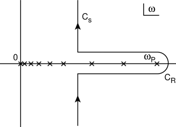
Figure 1: Integration contour $C_{R}+C_{s}$ for the Green’s function decomposition in Eq. (12). $C_{R}(C_{s})$ refers to the Pomeron (perturbative) contribution.

Our goal in the following is to analyze in more detail the $Y$-dependence in Eq. (14), by determining the regime in which the exponent $\omega_{s}$ is relevant, and the magnitude and form of diffusion corrections to it.

3 Diffusion features of the Airy model: a heuristic
approach

We have just clarified that the two terms in the decomposition (2) generate the $Y$-dependence in $G(Y;k,k_{0})$ in a quite different way. The non-perturbative (Pomeron) term provides just a Regge-pole behaviour $\sim\exp(\omega_{P}Y)$, while the perturbative one is analogous to a “background integral” (Fig. 1) and will generate a non-trivial exponent only if the small-$\omega$ oscillations of ${\cal F}$ and $\tilde{\cal F}$ are kept in phase by the $\omega$-integration. By writing, for the Airy model,

$$g_{P}(Y;t,t_{0})\equiv kk_{0}~{}G_{P}=\int{d\omega\over 2\pi i}~{}e^{\omega Y}{\pi t_{0}\over\omega}~{}~{}\bigg{(}{2b\omega\over\chi^{"}_{m}}\bigg{)}^{2\over 3}Ai(\xi)~{}Bi(\xi_{0})~{},$$ (15)

we expect, for $\Delta t=t-t_{0}\ll t$ that phase relations are kept only if $\xi$ and $\xi_{0}$ are kept finite for large $Y$. By the definition (11), this implies that $\omega-\omega_{s}(t)\simeq\omega-\omega_{s}(t_{0})=0(t^{-{5\over 3}})$ are small parameters. Furthermore, in this region, by Eq. (11),

$$\xi\simeq D^{-{1\over 3}}t^{{2\over 3}}~{}~{}\bigg{(}{\omega\over\omega_{s}(t)}-1\bigg{)}$$ (16)

is just linear in $\omega-\omega_{s}$. By replacing the linearized expression (16) into Eq. (15), we can rewrite it in the form

$$g_{P}(Y;t,t_{0})\simeq\pi(Dt)^{-{1\over 3}}e^{\omega_{s}(t)Y}~{}~{}\int^{+i\infty}_{-i\infty}~{}{d\xi\over 2\pi i}~{}e^{\xi\eta}Ai(\xi)Bi(\xi-\delta)~{},$$ (17)

where we have introduced the parameters

$$\eta=D^{{1\over 3}}~{}Y~{}\omega_{s}(t)~{}t^{-{2\over 3}}\sim Yt^{-{5\over 3}}~{},~{}~{}~{}\delta=\Delta t(Dt)^{-{1\over 3}}~{}.$$ (18)

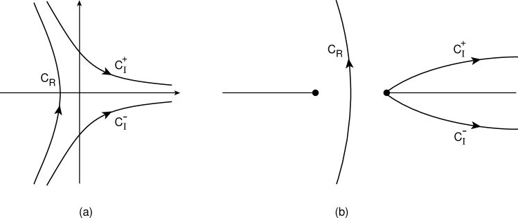
Figure 2: Contours in the $\nu=\gamma-{1/2}$ plane for ($C_{R}$) the regular and ($C_{I}$) the irregular solution in the case of ($a$) the Airy model and ($b$) the two-pole collinear model.

The integral in (17) can now be evaluated in a heuristic way by introducing the integral representations (Fig. 2a)

$$Ai(\xi)=\int_{C_{R}}~{}{d\nu_{A}\over 2\pi i}~{}e^{\nu_{A}\xi-{1\over 3}\nu_{A}^{3}}~{},Bi(\xi)=\int_{C_{I}^{+}+C^{-}_{I}}~{}{d\nu_{B}\over 2\pi}~{}e^{\nu_{B}\xi-{1\over 3}\nu_{B}^{3}}~{}$$ (19)

and by performing the $\xi$-integration under the integral, to yield a delta-function. We thus obtain

$$I(\eta,\delta)\equiv\int~{}{d\xi\over 2\pi i}~{}e^{\xi\eta}~{}Ai(\xi)~{}Bi(\xi-\delta) = \int^{+i\infty}_{-i\infty}~{}{d\nu_{A}\over 2\pi^{2}i}~{}\exp\bigg{(}\eta\nu^{2}_{A}+(\eta^{2}+\delta)\nu_{A}+\eta\delta+{\eta^{3}\over 3}\bigg{)}$$ (20)

$$= {1\over 2\pi\sqrt{\pi\eta}}~{}\exp\bigg{(}{\eta^{3}\over 12}+{\eta\delta\over 2}-{\delta^{2}\over 4\eta}\bigg{)}~{}.$$

By inserting Eqs. (20) and (18) into Eq. (17), we finally get

$$g_{P}(Y,t,t_{0})={1\over\sqrt{4\pi D\omega_{s}(t)Y}}~{}\exp\bigg{[}\omega_{s}(t)Y\bigg{(}1+{\Delta t\over 2t}\bigg{)}-{(\Delta t)^{2}\over 4D\omega_{s}(t)Y}+{\eta^{3}\over 12}\bigg{]}$$ (21)

which provides the diffusion and running coupling corrections to the hard Pomeron behaviour.

There are two features worth noting in Eq. (21), in comparison with the customary expression with frozen coupling. Firstly, the exponent $\omega_{s}$ is corrected by a term linear in $\Delta t=t-t_{0}$ which provides the symmetrical argument $\omega_{s}({t+t_{0}\over 2})$ in the running coupling, as is appropriate for the factorized scale $\sim kk_{0}$ already introduced in eq. (12). Furthermore, the exponent carries the diffusion correction $\eta^{3}\sim Y^{3}/t^{5}$, which is of relative order $Y^{2}/t^{4}$ compared to the leading term $\omega_{s}(t)Y$. This correction was obtained as running coupling effect in [6], [7],[8]and confirmed [9] in the models considered here under the assumption $\eta\ll 1$, or $Y\ll t^{{5\over 3}}$.

The question then arises of the boundary of validity of the heuristic argument presented above. We shall see in Section 4 that the assumption $\eta\ll 1$ can be relaxed, and replaced by $\eta\ll t^{{1\over 3}}$, or $Y\ll t^{2}$. For $Y\mathrel{\hbox to0.0pt{\raise 2.15277pt\hbox{$>$}\hss}{\lower 2.15277pt\hbox{$\sim$}}}t^{2}$ on the other hand, the linearization in Eq. (14) breaks down, and the integral in Eq. (13) enters a new regime in which it first decreases, and then starts oscillating (Section 5), so that the phase relations are lost.

A first hint at such behaviour is obtained by replacing the ansatz in Eq. (21) in the diffusion equation

$${\partial\over\partial Y}~{}g_{P}(Y,t,t_{0})\simeq\omega_{s}(t)~{}\bigg{(}1+D\partial^{2}_{t}\bigg{)}~{}g_{P}(Y,t,t_{0})~{}.$$ (22)

In fact, the $Y$-derivative of the exponent $E(Y,t,\Delta t)=\log g_{P}$ is given by

$${\partial E(Y,t,\Delta t)\over\partial Y}=-{1\over 2Y}+\omega_{s}(t)~{}\bigg{(}1+{\Delta t\over 2t}\bigg{)}+{(\Delta t)^{2}\over 4D\omega_{s}Y^{2}}+{\partial\over\partial Y}~{}\bigg{(}{\eta^{3}\over 12}\bigg{)}$$ (23)

and should match the right-hand side of Eq. (22), which is given by

$$\omega_{s}(t)\bigg{[}1+D\bigg{(}({\partial\over\partial t}E)^{2}+{\partial^{2}E\over\partial t^{2}}\bigg{)}\bigg{]}~{},$$

$${\partial E\over\partial t}=-{1\over 2t}\omega_{s}(t)Y(1+{\Delta t\over t})-{\Delta t\over 2D\omega_{s}Y}~{}(1+2{\Delta t\over t})+{\partial\over\partial t}~{}({\eta^{3}\over 12})+{1\over 2t}~{}.$$ (24)

If we keep terms of relative order $t/Y$, $\Delta t/t$, $Y^{2}/t^{4}$ (such terms are all of the same order for fixed values of $\eta$), we find that Eqs. (23) and (24) are indeed consistent, provided

$${\partial\over\partial Y}~{}~{}{\eta^{3}\over 12}=D{\omega^{3}_{s}Y^{2}\over 4t^{2}}~{},$$ (25)

thus reproducing the expression (18) for $\eta(Y,t)$. But, because of (25), we also generate from Eq. (22) terms of relative order $Y^{4}/t^{8}$ which are subleading only if $Y\ll t^{2}$, and do not check with Eq. (23). Therefore, the heuristic argument breaks down for $Y=0(t^{2})$.

4 Detailed analysis of the regime $t<Y\ll t^{2}$

In this section we give a more complete evaluation of the integral (15) which defines $g_{P}$ and in doing so we confirm the result (21) and its validity boundary, obtained in a heuristic way in the previous section.

4.1 Choice of integration contour

We begin with the $\omega$-integration contour in (13) being parallel to the imaginary $\omega$-axis with Re$\omega=\omega_{s}$ (Fig. 3). In order to effectively separate leading from non-leading behaviours in (13) it is convenient to use different forms of the product $Ai(\xi)~{}Bi(\xi_{0})$ for Im$\omega>0$ and for Im$\omega<0$. To that end we write

$$Ai(\xi)Bi(\xi_{0})=\mp{2i\sqrt{\xi\xi_{0}}\over 3\pi^{2}}~{}K_{{1\over 3}}({2\over 3}\xi^{{3\over 2}})~{}\bigg{[}K_{{1\over 3}}({2\over 3}\xi_{0}^{{3\over 2}}e^{\mp i\pi})-{1\over 2}~{}K_{{1\over 3}}({2\over 3}\xi_{0}^{{3\over 2}})\bigg{]}$$ (26)

where the upper (lower) sign will be the form used in (13) when Im$\omega>0(<0)$. Equation (26) follows from (8) and (10) along with

$$K_{\nu}(e^{i\pi}\zeta)+K_{\nu}(e^{-i\pi}\zeta)=2\cos\pi\nu K_{\nu}(\zeta)~{}.$$ (27)

Thus

$$g_{P}(Y_{;}t,t_{0})=\bar{g}_{P}(Y;t.t_{0})+R(Y;t,t_{0})$$ (28)

with

$$\bar{g}_{P}(Y;t,t_{0})=\int\mp{t_{0}d\omega\over 3\pi^{2}\omega D}~{}\sqrt{({\omega\over\omega_{s}(t)}-1)~{}({\omega\over\omega_{s}(t_{0})}-1)}~{}~{}e^{\omega Y}K_{{1\over 3}}({2\over 3}\xi^{{3\over 2}})~{}K_{1\over 3}({2\over 3}\xi_{0}^{{3\over 2}}e^{\mp i\pi})$$ (29)

and

$$R(Y;t,t_{0})=\int\pm{t_{0}d\omega\over 6\pi^{2}\omega D}~{}\sqrt{({\omega\over\omega_{s}(t)}-1)~{}({\omega\over\omega_{s}(t_{0})}-1)}~{}~{}e^{\omega Y}K_{{1\over 3}}({2\over 3}\xi^{{3\over 2}})~{}K_{1\over 3}({2\over 3}\xi_{0}^{{3\over 2}})$$ (30)

where the upper (lower) sign is to be used when Im$\omega>0(<0)$.

We shall first show that $R$ can be chosen small compared to $\bar{g}_{0}$ by a judicious contour deformation. Since the integrand of (24) decreases for positive real $\xi$, we are led to deform $C_{s}$ around the real $\xi$ axis to reach a point $\xi_{1}>1$ to be defined below. In estimating the size of $R$ we shall take $\xi_{0}\approx\xi$ so that the full exponent appearing in (30), in the region where $|\xi|\gg 1$ where the asymptotic form of $K_{{1\over 3}}$ can be used, is

$${\cal E}=\omega_{s}(t)Y+(\omega-\omega_{s}(t)Y-{4\over 3}\xi^{{3\over 2}}~{}.$$ (31)

In the region where $\xi\ll t^{{2\over 3}}$

$${\cal E}-\omega_{s}Y\simeq\xi\eta-{4\over 3}\xi^{{3\over 2}}~{}.$$ (32)

Thus we can make the second term on the right-hand side of (32) dominate the first term at $\xi=\xi_{1}$ if

$$\xi_{1}/\eta^{2}\gg 1~{}.$$ (33)

We note that (33) is possible, keeping $\xi_{1}\ll t^{2/3}$, so long as $\eta\ll t^{{1\over 3}}$ or, equivalently, so long as $Y\ll t^{2}$. We anticipate $\bar{g}_{P}$ being of size $e^{\omega_{s}Y}$ so that if we are able to choose an integration path in (24) having Re${4\over 3}\xi^{{3\over 2}}\gg(\omega-\omega_{s})Y$, then $R$ can be neglected.

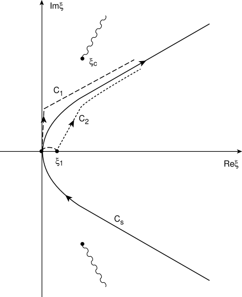
Figure 3: Integration contours in the $\xi$ plane, cut at $\xi_{c}\sim t^{2/3}$. $C_{s}$ corresponds to Re$\omega=\omega_{s}$. The dashed (dotted) contour $C_{1}$ ($C_{2}$) corresponds to the deformed contour defined in the text. The corresponding ones in Im$\xi<0$ are not shown

A contour of this kind is $C_{2}$ in Fig. 3. It is basically a deformation of the contour $C_{s}$ at Re$\omega=\omega_{s}$ in order to have $\xi_{1}$ as starting point and to depart from it with Arg$(\xi-\xi_{1})<{\pi\over 3}$. Its basic property is to lie completely within the regions $|\rm Arg\xi|<{\pi\over 3}$, such that the product of regular Airy functions is damped (Re$\xi^{{3\over 2}}>0)$. It is then easy to convince oneself that Re$({4\over 3}\xi^{{3\over 2}})\gg$ Re$(\omega-\omega_{s})Y$ on a contour of this kind, so that the contribution $R$ in Eq (30) can be neglected compared to $\bar{g}_{P}$ so long as $Y\ll t^{2}$.

4.2 From the $\omega$-integral to the $\xi$-integral

Our task is now to evaluate (29) and to specify once again a convenient path of integration in $\xi$, that will turn out to be different from that chosen before. We are able to evaluate (29) only in a linear approximation of $\xi$ and $\omega-\omega_{s}(t)$, and we first turn to a more complete justification of this approximation. When $|\xi_{0}|$ and $|\xi|$ are large, the terms appearing in the exponent in (29) are

$${\cal E}=\omega Y-{2\over 3}\xi^{{3\over 2}}+{2\over 3}\xi_{0}^{{3\over 2}}~{}.$$ (34)

This can be written as

$${\cal E}=\omega_{s}(t)Y+\xi\eta\bigg{(}{\omega\over\omega_{s}}\bigg{)}^{{2\over 3}}-{2\over 3}~{}\xi^{{3\over 2}}+{2\over 3}(\xi-\delta\bigg{(}{\omega\over\omega_{s}}\bigg{)}^{{1\over 3}})^{{3\over 2}}~{},$$ (35)

with $\delta$ as given in (18). The linear approximation gives

$${\cal E}_{\rm lin}=\omega_{s}(t)Y+\xi\eta-{2\over 3}~{}\xi^{{3\over 2}}+{2\over 3}(\xi-\delta)^{{3\over 2}}~{},$$ (36)

In order to see how close ${\cal E}$ and ${\cal E}_{\rm lin}$ are, we deform $C_{s}$ to the contour $C_{1}$, in this case (Fig. 3). The latter, departing from $\xi_{1}$ and reaching the origin, is chosen in such a way as to run over the imaginary $\xi$ axis in the whole linearization region $|\rm Im\xi|<t^{{2\over 3}}$, and to approach $C_{s}$ later on in the Re$\omega<\omega_{s}$ region. It is straightforward to see that the regions of $C_{1}$ on the real and imaginary axis are the dominant ones in the integral. In fact, from Eq. (36) one sees that Re$({\cal E}_{\rm lin}-\omega_{s}Y)$ vanishes at $\xi=0$ and decreases steadily below zero for $\xi$ on the imaginary axis. Furthermore, in the asymptotic region where $C_{1}$ starts approaching $C_{s}$ the Airy phase is negligible and the integrand in Eq. (29) is damped because of Re$\omega<\omega_{s}$.

Now we want to replace ${\cal E}$ by ${\cal E}_{\rm lin}$ in the exponent. We can estimate the error in the exponent by comparing (35) and (36) in the region $0\leq\xi\leq\xi_{1}$. The maximum deviation occurs for $\xi=\xi_{1}$ and the size of the deviation is

$$\Delta{\cal E}={\cal E}-{\cal E}_{\rm lim}\simeq\xi_{1}\eta\bigg{[}\bigg{(}{\omega\over\omega_{s}}\bigg{)}^{{2\over 3}}-1\bigg{]}-\sqrt{\xi_{1}}\delta\bigg{[}\bigg{(}{\omega\over\omega_{s}}\bigg{)}^{{1\over 3}}-1\bigg{]}~{}.$$ (37)

From (11) one sees $\bigg{[}\bigg{(}{\omega\over\omega_{s}}\bigg{)}^{{1\over 3}}-1\bigg{]}$ and $\bigg{[}\bigg{(}{\omega\over\omega_{s}}\bigg{)}^{{2\over 3}}-1\bigg{]}$ are of size $\xi_{1}t^{-2/3}$, so that $\Delta{\cal E}$ has terms of size $\xi_{1}^{2}\eta t^{-2/3}$ and $\xi^{3/2}_{1}{\Delta t/t}$. Taking $\xi_{1}=N\eta^{2}$ for $N$ large, the smallest we are allowed to take $\xi_{1}$, and taking $\Delta t\simeq(Dt)^{{1\over 3}}\eta^{2}$ as region of $\Delta t$ where $g_{P}$, as given in (19), take its maximum value we find

$$\Delta{\cal E}\approx{\eta^{5}\over t^{{2\over 3}}}~{}~{},~{}~{}\sim\omega_{s}Y{Y^{4}\over t^{8}}.$$ (38)

Thus we can expect our final result and have errors of size $\Delta{\cal E}$ in the exponent.

In changing the exponent ${\cal E}$ in (29) to ${\cal E}_{\rm lin}$ we take the same contour as indicated in Fig. 3, but now the integration is continued along the imaginary $\xi$-axis up to $\xi=i\infty$. Using the linearized form for $d\xi$ also induces an error in the prefactor of the dominant exponential of size ${\omega-\omega_{s}\over\omega_{s}}\propto\bigg{(}{\eta\over t^{{1\over 3}}}\bigg{)}^{2}\sim{Y^{2}\over t^{4}}$ compared to 1. Thus, finally, the integration which we need to evaluate is

$$g_{P}(Y;t,t_{0})=\mp[Dt]^{-{1\over 3}}e^{\pm i{\pi\over 3}}e^{\omega_{s}(t)Y}~{}~{}\int_{C_{1}}d\xi~{}e^{\eta\xi}~{}Ai(\xi)Ai\bigg{(}(\xi-\delta)e^{\mp 2i{\pi\over 3}}\bigg{)}$$ (39)

where we have used (8) to express the $K_{{1\over 3}}$ functions appearing in (23) by Airy functions for reasons which will become clear in a moment. The integration is taken with the contour $C_{1}$ extended to $\pm i\infty$, with, as usual, the upper (lower) sign referring to Im$\xi$ greater (less) than zero.

4.3 Evaluation of the $\xi$-integrals

In order to evaluate the integral in (39) it is convenient to define

$$I_{\pm}=\int^{\pm i\infty}_{\xi_{1}\pm i\epsilon}d\xi~{}e^{\eta\xi}P_{\pm}(\xi)~{},~{}~{}~{}J_{\pm}=\int^{\pm i\infty}_{\xi_{1}\pm i\epsilon}d\xi~{}e^{\eta\xi}Q_{\pm}(\xi)~{},$$ (40)

$$P_{\pm}(\xi)=U(\xi)V_{\pm}(\xi-\delta)~{},~{}~{}~{}Q_{\pm}(\xi)={\partial\over\partial\xi}U(\xi)V_{\pm}(\xi-\delta)~{},$$ (41)

with

$$U(\xi)=Ai(\xi)~{},~{}~{}~{}V_{\pm}(\xi)=\mp e^{\pm i{\pi\over 3}}~{}Ai((\xi-\delta)~{}e^{\mp 2i{\pi\over 3}})~{}.$$ (42)

Using ${d^{2}\over d\xi^{2}}U(\xi)\equiv U^{\prime\prime}(\xi)=\xi U(\xi)$ and $V_{\pm}^{\prime\prime}(\xi-\delta)=(\xi-\delta)V_{\pm}(\xi-\delta)$ one can show that

$$P^{\prime\prime\prime}=[4\xi P-\delta P]^{{}^{\prime}}-2P-2\delta Q~{},~{}~{}~{}Q^{\prime\prime}=2(\xi P)^{{}^{\prime}}-P-\delta Q$$ (43)

from which, by integration by parts, one finds

$$2I = -\eta[4{\partial\over\partial\eta}-\delta-\eta^{2}]~{}I-2\delta J+e^{\eta\xi_{1}}P_{2}(\xi_{1},\eta)~{},$$

$$J(\delta+\eta^{2})+I = -2\eta{\partial I\over\partial\eta}+e^{\eta\xi_{1}}Q_{2}(\xi_{1}\eta)~{},$$ (44)

where the $\pm$ indices have been suppressed in (43)-(45). Also

$$P_{2} = P^{\prime\prime}(\xi_{1})-\eta P^{{}^{\prime}}(\xi_{1})+\eta^{2}P(\xi_{1})-(4\xi_{1}-\delta)P(\xi_{1})~{},$$

$$Q_{2} = Q^{{}^{\prime}}(\xi_{1})-2\xi_{1}P(\xi_{1})-\eta Q(\xi_{1})~{}.$$ (45)

Using Eq. (44), one easily finds

$$\bigg{[}\eta{\partial\over\partial\eta}+{1\over 2}-{(\delta+\eta^{2})^{2}\over 4\eta}\bigg{]}~{}I_{\pm}={e^{\eta\xi_{1}}\over 4\eta^{2}}\bigg{[}(\delta+\eta^{2})P_{2\pm}-2\delta Q_{2\pm}\bigg{]}=S_{\pm}$$ (46)

The solution to (46) is

$$I_{\pm}={1\over\sqrt{\eta}}~{}\exp\bigg{[}{\eta^{3}\over 3}-{(\delta-\eta^{2})^{2}\over 4\eta}\bigg{]}~{}\bigg{(}C_{\pm}+\int^{\eta}_{\eta_{0}}~{}{d\eta^{{}^{\prime}}\over\sqrt{\eta^{{}^{\prime}}}}~{}\exp\bigg{[}-{\eta^{{}^{\prime}3}\over 3}+{(\delta-\eta^{{}^{\prime}2})^{2}\over 4\eta^{{}^{\prime}}}\bigg{]}S_{\pm}(\eta^{{}^{\prime}}\bigg{)}$$ (47)

with $C_{\pm}$ a constant to be determined. Referring back to (39) one can write

$$g_{P}(Y;t,t_{0})=(D^{2}t)^{-{1\over 3}}~{}e^{\omega_{s}(t)Y}~{}(I_{+}-I_{-})~{}.$$ (48)

Now the combination $S_{+}-S_{-}$ occurring in the integrand of the particular solution of (47) which enters in (48) always involves the combination

$$K_{1\over 3}({2\over 3}(\xi_{1}-\delta)^{3\over 2}~{}e^{-i\pi})+K_{1\over 3}({2\over 3}(\xi_{1}-\delta)^{3\over 2}~{}e^{+i\pi})=K_{1\over 3}({2\over 3}(\xi_{1}-\delta)^{3\over 2})\propto\exp[-{2\over 3}(\xi_{1}-\delta)^{3\over 2}]$$

so that the particular solution can be ignored. Although we have focused here on $\eta$ large the procedure also should be valid when $\eta\ll 1$. For $\eta\ll 1$, the first factor in (47), ${1\over\sqrt{\eta}}\exp[-{\delta^{2}\over 4\eta}]$, gives the usual BFKL diffusion which means that $C_{+}-C_{-}$ can be determined by evaluating $I_{+}-I_{-}$ when $\delta=0$ and when $\eta$ is small. One finds

$$C_{+}-C_{-}={1\over\sqrt{4\pi}}$$ (49)

giving exactly the result (21)

$$g_{P}(Y;t,t_{0})~{}=~{}{1\over\sqrt{4\pi D\omega_{s}(t)Y}}~{}e^{\omega_{s}(t)Y-{1\over 4\eta}(\delta-\eta^{2})^{2}+{\eta^{3}\over 3}}$$ (50)

In arriving at this result we have chosen to expand the integrand of (29) about $\xi$ and $t$ and then integrate over $\xi$. Alternatively, if the expansion had been about $\xi_{0}$ and $t_{o}$ with the integration over $\xi_{0}$ the result

$$g_{P}(Y;t,t_{0})={1\over\sqrt{4\pi D\omega_{s}(t_{0})Y}}~{}e^{\omega_{s}(t_{0})Y-{1\over 4\eta_{0}}(\delta_{0}-\eta^{2}_{0})^{2}+{\eta^{3}_{0}\over 3}}$$ (51)

would have been obtained with $\eta_{0}=Y\omega_{s}(t_{0})D^{{1\over 3}}t_{0}^{-{2\over 3}}$ and with $\delta_{0}=(t_{0}-t)~{}(Dt_{0})^{-{1\over 3}}$. The difference of these exponents is

$${\delta_{0}\eta_{0}-\delta\eta\over 2}-{1\over 4}~{}\bigg{(}{\delta^{2}\over\eta}-{\delta^{2}_{0}\over\eta_{0}}\bigg{)}+{\eta^{3}-\eta_{0}^{3}\over 12}=\Delta~{}.$$ (52)

When ${\Delta t\over t}\ll 1$,

$$\Delta\simeq\delta(Dt)^{{1\over 3}}~{}{d\over dt}~{}\bigg{(}{\delta\eta\over 2}-{\delta^{2}\over 4\eta}+{\eta^{3}\over 12}\bigg{)}~{}.$$ (53)

Using $\delta\propto\eta^{2}$ as the important values of $\delta$ in (50), one easily finds

$$\Delta\propto{\eta^{5}\over t^{{2\over 3}}}\sim\omega_{s}Y({Y^{4}\over t^{8}})$$ (54)

which is exactly the size of the error estimated in (32). This conclusion is consistent with the estimate ${\Delta\over\omega_{s}Y}=0({Y^{4}\over t^{8}})$ obtained from the heuristic argument based on Eq. (22).

5 The very large $Y$ regime

In the previous section we have exploited the decomposition (28) of the Green’s function in two terms, one (Eq. (29)) with product of Airy functions out of phase $(\sim K(\xi)K(e^{\mp i\pi}\xi_{0}))$, and the other in phase $(\sim K(\xi)K(\xi_{0})$, Eq. (30)), corresponding to the exponents

$${\cal E}(\omega,Y)=\omega Y-{3\over 2}\xi^{{3\over 2}}\pm{3\over 2}\xi^{{3\over 2}}_{0}~{}.$$ (55)

We have shown that, for $Y\ll t^{2}$, the integral is dominated by Re$\omega\simeq\omega_{s}$, the contribution (30) being negligible on a contour with a slight deformation in Re$\omega>\omega_{s}$. On the other hand, for $Y\gg t^{2}$, it becomes profitable to distort the contour in Re$\omega<\omega_{s}$, where the contribution (30) becomes actually dominant, because Re$\xi^{{3\over 2}}$ may take negative values.

In fact, for small enough $\omega$ in Im$\omega{>\atop<}0$, the exponent with ($-$) sign in Eq. (55) takes the form

$${\cal E}_{\pm}\simeq\omega Y\pm{4i\over 3}~{}{t\omega_{s}(t)\over D\omega}$$ (56)

with derivatives

$${d{\cal E}_{\pm}\over d\omega}=Y\mp{4i\over 3}~{}{\chi_{m}\over b{\sqrt{D}}\omega^{2}}~{},~{}~{}~{}{d^{2}{\cal E}_{\pm}\over d\omega^{2}}=\pm{8i\over 3}~{}{\chi_{m}\over b\sqrt{D}\omega^{2}}~{},$$ (57)

Therefore, there are saddle points of the exponent (56) at

$$\omega_{\pm}=\sqrt{{2\over 3}}(1\pm i)~{}\bigg{(}{\chi_{m}\over bY\sqrt{D}}\bigg{)}^{{1\over 2}}$$ (58)

with

$${d^{2}{\cal E}_{\pm}\over d\omega_{\pm}^{2}}=(1\mp i)~{}\bigg{(}{3b\sqrt{D}\over 2\chi_{m}}\bigg{)}^{{1\over 2}}Y^{{3\over 2}}~{}.$$ (59)

Since $(d^{2}{\cal E}_{\pm}/d\omega^{2}_{\pm})^{-{1\over 2}}\ll\omega_{\pm}$ the gaussian integration, in (24), about the saddle points should be an accurate evaluation of the integral. One finds

$$g_{P}(Y;t,t_{0})={t_{0}\over 3\sqrt{\pi}}~{}\bigg{(}{3b\over 4\chi_{m}D^{5/6}Y}\bigg{)}^{{3\over 4}}~{}\bigg{[}\cos(\bar{\omega}\sqrt{Y}+{\pi\over 8})\bigg{]}e^{\bar{\omega}\sqrt{Y}}~{},$$ (60)

with $\bar{\omega}^{2}={8\chi_{m}\over 3b\sqrt{D}}$.

It then appears that the perturbative solution becomes smaller than predicted by the exponent $\omega_{s}(kk_{0})Y$ (because $\sqrt{Y}\ll\omega_{s}Y$ for $Y\gg t^{2}$) and furthermore it starts oscillating, thus loosing positivity. It is no surprise that, at such large $Y$ values, our perturbative calculation no longer has physical sense. After all, when $Y$ approaches $t^{2}$ from below it is clear from (21), or (50), that $\Delta t$ approaches $t$ at which point one expects the singular potential evident in (5) to become troublesome. That is, when $Y$ approaches $t^{2}$ the cutoff at $\bar{t}$ is clearly necessary. Two questions then arise: firstly, whether we can still describe the behaviour of $g_{P}$ in the intermediate region $Y~{}\propto~{}t^{2}$; and, secondly, at which $Y$ values does the non-perturbative Pomeron part really take over.

We are unable to answer either question in detail. However, for the pure Airy model described by Eq. (22), we can provide a partial resummation of the corrections to the exponent of relative order $(Y/t^{2})^{2n}$ as follows. Referring to Eq. (24) we first neglect, in the large $Y$ regime, the term ${\partial^{2}E\over\partial t^{2}}$ compared to $({\partial E\over\partial t})^{2}$; then we consider the exponent $E(Y;t,\Delta t)$ around its maximum in $\Delta t$ so as to neglect its $\Delta t$ derivative, and we take the ansatz

$$E(Y;t,\Delta t_{\rm max})=\omega_{s}(t)Y~{}f(z),~{}~{}z=D\chi_{m}{Y^{2}\over t^{4}}={{\eta}^{3}\over{\omega_{s}Y}}~{}.$$ (61)

which is supposed to describe the $Y^{2}/t^{4}$ dependence. Finally, by replacing Eq. (61) into Eq. (22), we get the non-linear differential equation

$$f(z)+2zf^{\prime}(z)~{}=~{}1+z[f(z)+4zf^{\prime}(z)]^{2}~{},$$ (62)

which is a sort of Hamilton-Jacobi limit of the diffusion equation (22).

For $z\ll 1$ ($Y\ll t^{2}$), the iterative solution to Eq. (62) is $f(z)=1+z/3+2z^{2}/3+...$, which yields the ${\eta^{3}/3}$ term of Eq. (50) and the first non-trivial correction to it. On the other hand, for $z\gg 1$ ($Y\gg t^{2}$), Eq. (62) still makes sense, with a solution $f(z)\sim z^{-1/4}+O(z^{-1/2})$, in order to compensate the term $1$ in the r.h.s. Therefore, since $z\propto Y^{2}/t^{4}$, the exponent in Eq (61) turns out to be in agreement with the saddle point estimate in Eq. (60). Note, however that while the behaviour (50) is supposed to be universal for $Y\ll t^{2}$ (Cf. Sec. 6), the resummation in Eq. (62) and the large $Y$ regime in Eq. (60) are typical of the Airy model, because they involve large $\xi$ properties of Eq. (22).

We wish now to compare the large $Y$ behaviour of the perturbative term in Eqs. (21) and (50) - with its intricate transition to the behaviour (60) just discussed - to the non-perturbative Pomeron term. The latter can only be discussed in a model dependent way. In the Airy model defined in Eqs (8) and (9) it is straightforward to show that

$$g_{R}(Y;t,t_{0})~{}\simeq~{}e^{\omega_{P}Y}{\pi t_{0}\over\omega_{P}}\bigg{(}{2b\omega_{P}\over\chi_{m}^{\prime\prime}}\bigg{)}^{2/3}~{}Ai^{2}(\xi_{P})\simeq\exp[{\omega_{P}Y-{4\over 3}t^{3/2}\bigg{(}{b\omega_{P}\over{\chi_{m}D}}\bigg{)}^{1/2}}],$$ (63)

where $\xi_{P}\sim t(b\omega_{P}/\chi_{m}D)^{1/3}$ and we have assumed $\omega_{P}\gg\omega_{s}(t)$, for definiteness. It is clear from Eq. (63) that the Pomeron term is exponentially suppressed with respect to the perturbative one for large $t$. However, it takes over at very large energies, such that

$$Y~{}>~{}Y_{c}\simeq{4t^{3/2}\over 3\omega_{P}}\bigg{(}{b\omega_{P}\over{\chi_{m}D}}\bigg{)}^{1/2}~{},$$ (64)

that is, even before the region $Y\simeq t^{2}$ is reached, as already pointed out for collinear models in [9].

The above estimate of $Y_{c}$ is model dependent in several ways. In fact the weight of the Pomeron term depends on the small-$x$ equation being used (cf. Sec. (6)) and, within the given equation, on the way the strong coupling region is smoothed out or cutoff [10]. Furthermore, unitarity corrections may affect it, and there is no consensus on how to incorporate them. However, the basic qualitative feature underlying all models is that “tunneling” to the Pomeron behaviour occurs at some $Y_{c}<t^{2}$, i. e. before the perturbative calculation looses sense, thus insuring cross-section positivity.

6 Extension to collinear small-$x$ models

The above evaluation of perturbative diffusion properties of the Airy model (Eqs. (21) and (50)) can be generalized to other small-$x$ models, for which the expression (12) of the perturbative Green’s function is sufficiently explicit.

For instance, a simple two-pole collinear model [9] is provided by the effective eigenvalue function

$$\chi(\gamma,\omega)={1\over\gamma}+{1\over 1+\omega-\gamma}~{},$$ (65)

where we have introduced the $\omega$-shift [12], but no further subleading terms. The corresponding Green’s function is defined by [11]

$$[\omega-\chi({1\over 2}+\partial_{t},\omega){1\over bt}]~{}g_{\omega}(t,t_{0})=\delta(t-t_{0})~{},$$ (66)

which basically provides a second order differential equation for $g_{\omega}$. Therefore, the solution is of type in Eq. (2), which, for $t>t_{0}>\bar{t}$, reads

$$g_{\omega}(t,t_{0}) = {1\over\omega}~{}\delta(t-t_{0})+{1\over\omega^{2}bt_{0}}~{}W_{{1\over b\omega},{1\over 2}}\bigg{[}(1+\omega)t\bigg{]}\times$$ (67)

$$\times\bigg{[}W_{-{1\over b\omega},{1\over 2}}(-(1+\omega)t_{0})+S(\omega)W_{{1\over b\omega},{1\over 2}}((1+\omega)t_{0})\bigg{]}~{}.$$

Here $W_{k,m}(z)$ is the Whittaker function, satisfying the Coulomb-like differential equation

$$\bigg{[}-{d^{2}\over dz^{2}}-{k\over z}+{m^{2}-{1\over 4}\over z^{2}}+{1\over 4}\bigg{]}~{}W_{l,m}(z)=0$$ (68)

and its “irregular” counterpart “$W_{-k,m}(z)$” is more precisely defined by the real analytic continuation

$$W_{-k}(-z)={1\over 2}~{}\bigg{(}e^{i\pi k}W_{-k}(e^{i\pi}z)+e^{-i\pi k}W_{-k}(e^{-i\pi}z)\bigg{)}~{}.$$ (69)

Such solutions admit also the $\gamma$-reresentation [10]

$$W_{\pm{1\over b\omega},1/2}\bigg{(}\pm(1+\omega)t\bigg{)}=\int_{C_{R},C_{I}}{d\gamma\over 2\pi i}~{}~{}e^{(\gamma-{1\over 2}t-{1\over b\omega}~{}X(\gamma,\omega)}$$ (70)

where $C_{R}(C_{I})$ is the contour for the regular (irregular) solution shown in Fig. 2b, and $\chi(\gamma,\omega)={\partial\over\partial\gamma}X(\gamma,\omega)$.

The energy dependence of the perturbative function $G_{P}(Y;t,t_{o})$ in Eq. (12) was already investigated in Refs. [10],[11] and is characterized by various regimes.

1. In the collinear limit $t\gg t_{0}>1$, and $Y\gg 1$, $G_{P}(Y;t,t_{0})$ is dominated by the customary anomalous dimension saddle point, which exists in the energy region

   $$\sqrt{{\log t/t_{0}\over bY}}\simeq\omega>\omega_{s}(t_{0})\gg\omega_{s}(t)~{},~{}~{}~{}(Y\equiv\log{s\over k^{2}})~{},$$ (71)

   where $\omega_{s}(t)={4\over(1+\omega_{s})bt}\simeq{4\over bt}$ is the saddle point exponent.

2. In the diffusion region $\Delta t=t-t_{0}\ll t$, and $Y\gg t\gg 1$, the important $\omega$ values drift towards $\omega_{s}(t)\simeq\omega_{s}(t_{0})$, and the asymptotic behaviour of the Green’s function matches a properly chosen Airy model.

In fact, if $t$ and ${1\over\omega}$ are both large, but $\omega-\omega_{s}(t)\simeq\omega-\omega_{s}(t_{0})$ is small, the phase in Eq. (70) is finite only if $(\gamma-{1\over 2})\sim(b\omega)^{{1\over 3}}$ is small also. This means that we are probing the region close to the minimum of $\chi(\gamma)$, in such a way that

$$\bigg{(}{2b\omega\over\chi_{m}^{\prime\prime}}\bigg{)}^{{1\over 3}}~{}~{}\bigg{(}t-{\chi_{m}\over b\omega}\bigg{)}=\xi=\bigg{(}{t\omega_{s}(t)\over\sqrt{D}\omega}\bigg{)}^{{2\over 3}}~{}~{}\bigg{(}{\omega\over\omega_{s}(t)}-1\bigg{)}$$ (72)

is finite. This is precisely the region where the $W$’s become asymptotically Airy functions, with parameters

$$\chi_{m}={4\over 1+\omega_{s}}~{},~{}~{}~{}D={\chi_{m}^{\prime\prime}\over 2\chi_{m}}={4\over(1+\omega_{s})^{2}}~{},~{}~{}~{}\omega_{s}(1+\omega_{s})={4\over bt}~{}.$$ (73)

For this reason, the linearized expression (15) holds in the present case also, under the same conditions.

The above argument shows that, in the region $t\ll Y\ll t^{2}$, and $(t-t_{0})\ll t$, the diffusion corrections of Eq. (19) are valid for the two-pole model also, and for any truncated model where the $\gamma$-representation (70) holds for both the regular and the irregular solution.

Of course, for $Y\gg t^{2}$, the important $\omega$ values become much smaller than $\omega_{s}(t)$, and the phases in Eq. (70) became stationary at $\chi(\bar{\gamma},\omega)=0$. For the Airy model this occurs at $\bar{\nu}=\bar{\gamma}-{1\over 2}\sim\pm{i\over\sqrt{D}}$, and provides the asymptotic behaviour used in Eq. (56). For the two-pole model, instead, $\bar{\gamma}$ drifts to $\pm i\infty$, and this provides the asymptotic formulas

$$g_{\omega} \sim \exp\bigg{(}\pm{2\pi i\over b\omega}\bigg{)}~{},$$

$$g_{P}(Y;t,t_{0}) \sim \exp\bar{\omega}\sqrt{Y}~{}\cos(\bar{\omega}\sqrt{Y}+{\pi\over 8})~{},$$ (74)

with $\bar{\omega}={4\pi\over b}$. Although the precise exponent is different, the qualitative behaviour (74) is the same as for the Airy model. This follows from the analogous structure of the $\gamma$-representation (69), with its $\exp({{\rm const}\over\omega})$ behaviour.

In conclusion, in the range $t\mathrel{\hbox to0.0pt{\raise 2.15277pt\hbox{$<$}\hss}{\lower 2.15277pt\hbox{$\sim$}}}Y\ll t^{2}$, the perturbative calculation shows a universal behaviour, described by Eq. (21) or Eq. (50) , where the only model dependence lies in the parameters $\chi_{m}$ and $D$, describing the hard Pomeron and the diffusion coefficient. For $Y\mathrel{\hbox to0.0pt{\raise 2.15277pt\hbox{$>$}\hss}{\lower 2.15277pt\hbox{$\sim$}}}t^{2}$ on the other hand, the perturbative behaviour is more model dependent and finally starts oscillating, thus loosing physical sense.

At some intermediate value $Y=Y_{c}$ ($t\ll Y_{c}\ll t^{2}$), the non-perturbative Pomeron takes over. We do not have a reliable model for such transition. Is it an abrupt “tunneling” effect [9], as in the two-pole model (with $\omega_{P}\gg\omega_{s}(t)$), or is it instead mediated by a long diffusion regime, as perhaps expected in unitarized models ($\omega_{P}\ll 1$)? This is an open question, which deserves further investigation.

References

- [1] L.N. Lipatov,Sov. J. Nucl. Phys. 23 (1976) 338; E.A. Kuraev, L. N. Lipatov and V. S. Fadin Sov. Phys. JETP 45 (1977) 199; Ya. Balitskii and L. N. Lipatov, Sov. J. Nucl. Phys.28 (1978) 822.
- [2] V. S. Fadin and L. N. Lipatov, Phys.Lett. 429B (1998) 127 and references therein.
- [3] G. Camici and M. Ciafaloni, Phys.Lett. 412B (1997) 396 and 430B (1998) 349.
- [4] J. C. Collins and J. Kwiecinski, Nucl.Phys. B316 (1989) 307.
- [5] G. Camici and M. Ciafaloni, Phys.Lett. B395 (1997) 318.
- [6] Yu. V. Kovchegov and A. H. Mueller, Phys.Lett. B439 (1998) 428.
- [7] N. Armesto, J. Bartels and M. A. Braun, Phys.Lett. B442 (1998) 459.
- [8] E. M. Levin, Nucl.Phys. 445B (1999) 481.
- [9] M. Ciafaloni, D. Colferai and G. P. Salam, JHEP 9910 (1999) 017 and 0007 (2000) 054.
- [10] M. Ciafaloni, D. Colferai and G. P. Salam, Phys.Rev. D60 (1999) 114036.
- [11] M. Taiuti, University of Firenze Thesis (2000), unpublished.
-
[12]
G. P. Salam,JHEP 9807 (1998) 19;
M. Ciafaloni, D. Colferai, Phys.Lett. 452B (1999) 372.